Regional Economic Development: An Economic Base Study and Shift-Share Analysis of Hays County, Texas

By

James Paul Quintero

An Applied Research Project (Political Science 5397)

Submitted to the Department of Political Science Texas State University

In Partial Fulfillment for the Requirements for the Degree of Masters of Public Administration

Fall 2007

Faculty Approval: ____________________________ Dr. Patricia M. Shields ____________________________ Dr. George Weinberger ____________________________ Ms. Stephanie Garcia, MPA

ii

About the Author James Quintero was born on February 26th, 1981 in San Jose, CA. After

completing his high school education in Houston, TX, he graduated from the University

of Texas at Austin in May 2004 with a B.A in Sociology. He is currently a graduate

research assistant, honor student, and a master of public administration candidate at

Texas State University – San Marcos.

Please feel free to contact James Quintero at JQ2401@hotmail.com with

questions or comments regarding this research.

iii

Acknowledgements

“Whether therefore ye eat, or drink, or whatsoever ye do, do all to the glory of God.” 1 Corinthians 10:31

Far and away the most difficult page of the ARP to write; this page does not do justice to all of the people who have helped me achieve my goals. To my Dad, your vision, persistence, and determination have been a driving force in my academic and personal life. Thank you for encouraging me to dream and never letting me give up. To my Mom, your counsel, guidance, understanding, and patience have given me an inner peace and strength which I draw upon daily. Thank you for allowing me the freedom to develop into the individual I am today – I know it has not been easy. To my friends and family, your support and enthusiasm have always been steadfast and trustworthy – I hope that I am fortunate enough to always have you at my side.

***A very special thanks to Dr. Patricia Shields – Your tutelage, direction, and

encouragement have been invaluable!*** Abstract

iv

The purpose of this paper is two-fold. First is to analyze the economy of Hays

County, Texas using the economic base study to determine the structure and composition of the local market. Using the location quotient technique as an indirect method of employment analysis, this research examines leading export industry sub-sectors to determine which industries “drive” the local economy by generating outside income for the community. The second is to analyze Hays County’s economy using shift-share analysis to compare regional growth against national development. The shift-share technique presents a supplemental aggregate data analysis method to strengthen the conclusions of the economic base study. The research findings conclude that Hays County is a rapidly growing region primarily dependent upon the retail, health care and social assistance, and manufacturing sectors to advance and maintain its economic development. As compared to the U.S. economy, the manufacturing sector is expanding locally while concurrently declining in the national marketplace. Given that the local manufacturing sub-sector is an integral component of employment propagation via export employment, the national decline of this industry in Hays County is significant.

TABLE OF CONTENTS

v

Acknowledgements iii

Abstract iv

Index of Figures and Tables vii

Chapter I – Introduction 1

Research Purpose 1

Summary of Chapters 1

Chapter II – Hays County, Texas 3

Chapter Overview 3

Regional Setting and Growth 3

The County Seat: San Marcos 8

Texas State University – San Marcos 10

Austin-San Antonio Corridor 12

Economic Development Models: A Synopsis 14

Chapter Summary 16

Chapter III – Literature Review 17

Chapter Overview 17

Economic Growth: A Governments Responsibility 17

Economic Base Analysis: An Introduction 19

Indirect Industry Classification: The Location Quotient 19

Clarifying the Export & Import Sectors 21

Direct vs. Indirect Classification 23

County Business Patterns 24

Export Employment Multiplier 26

Shift-Share Analysis: An Introduction 26

The National Growth Component 27

The Industrial Mix Component 28

The Competitive Share Component 28

Economic Base Analysis: Conceptual Framework Table 30

Shift-Share Analysis: Conceptual Framework Table 35

Chapter Summary 38

Chapter IV – Methodology 39

vi

Chapter Overview 39

North American Industrial Classification System 39

Economic Base Analysis: Operationalization Table 41

Shift-Share Analysis: Operationalization Table 42

Methodological Considerations 43

Design Strengths 44

Design Weaknesses 45

Human Subjects Protection 46

Chapter Summary 47

Chapter V – Results 48

Chapter Overview 48

Economic Base Analysis: Results 48

Export Employment Leaders 49

Export Employment Multiplier 51

Shift-Share Analysis: Results 52

Chapter Summary 58

Chapter VI – Conclusion 59

Chapter Overview 59

Chapter Findings 59

Final Considerations 61

Bibliography 62

Appendices Appendix A 68

Appendix B 76

Index of Figures and Tables

vii

Figure 2.1 – Hays County Statewide Setting 4

Figure 2.2 – Hays County Regional Setting 8

Table 2.1 – County Population Growth Comparisons 5

Table 2.2 – Business Development in Hays County: 1990 – 2005 6

Table 2.3 – Hays County’s Top 25 Major Private and Public Employers 7

Table 2.4 – Population Growth Projections 11

Table 3.1 – Conceptual Framework Table for an Economic Base Analysis 31

Table 3.1a – Economic Base Analysis Equations 31

Table 3.2 – Identifying Local and National Employment Estimates 32

Table 3.3 – Determining the Location Quotient 33

Table 3.4 – Calculating the Number of Export Employment Positions 34

Table 3.5 – Examining the Impact of the Export Base 35

Table 3.6 – Conceptual Framework Table for a Shift-Share Analysis 36

Table 3.6a – Shift-Share Analysis Equations 37

Table 4.1 – North American Industrial Classification System (NAICS) Example 41

Table 4.2 – Operationalization of the EBA Conceptual Framework Table 42

Table 4.3 – Operationalization of the SSA Conceptual Framework Table 43

Table 5.1 – Industry Results by NAICS Category 49

Table 5.2 – Industry Results by NAICS Industry 50

Table 5.3 - EEM Calculation for Hays County 2005 51

Table 5.4 – CS: Expanding Nationally and Declining Locally 53

Table 5.5 – CS: Declining Nationally and Expanding Locally 55

Table 5.6 – CS: Declining Nationally and Declining Locally 56

Table 5.7 – CS: Expanding Nationally and Expanding Locally 57

1

Regional Economic Development: An Economic Base Study and

Shift-Share Analysis of Hays County, Texas

Chapter I. Introduction Research Purpose

The purpose of this research project is to examine the local economy of Hays

County, Texas using two economic development models – the economic base study

(EBA) and the shift-share analysis (SSA). The objective of the economic base study is to

determine which industries generate actual economic growth and which industries

demonstrate growth potential. The goal of the shift-share analysis is to indicate the

relative economic growth rate of the region’s industries as compared to national trends

and determine the level of industrial diversification. This research further analyzes Hays

County’s population growth, business development, and regional setting to articulate its

geographic and economic significance.

Summary of Chapters

This applied research project consists of five primary chapters:

• Chapter two provides information on the regional setting of Hays County,

Texas and discusses its economic importance. Two economic growth

models – the economic base study and shift-share analysis –are introduced

as techniques used to aid policy makers in the decision-making and

planning processes.

2

• Chapter three reviews existing literature on the EBA and SSA techniques.

This chapter uses the literature to demonstrate the utility of the two

techniques as applied to a local economy.

• Chapter four discusses the methodologies used to perform the economic

analyses of Hays County. A primary focus of this chapter is the

construction of an EBA and SSA Operationalization Table. This chapter

also elaborates on the limitations of the EBA and SSA models.

• Chapter five analyzes the empirical outcomes of the models as they apply

to the local economy.

• Chapter six briefly summarizes the project findings and provides

recommendations using the results.

3

Chapter II. Hays County, Texas Chapter Overview

At the onset of this chapter, an overview of Hays County, Texas and the

surrounding region is presented. Key socioeconomic characteristics of the area, such as

current and projected population estimates, major industrial employers, and the on-going

development of the Austin-San Antonio corridor are highlighted to emphasize the

importance of studying this county. To conclude, this chapter introduces two economic

development models – the economic base analysis (EBA) and shift-share analysis (SSA)

– as a pair of reliable techniques to manage the region’s economic infrastructure.

Hays County: Setting and Growth

Located within a 200 mile radius of four of the fastest growing metropolitans in

the U.S. – Austin, San Antonio, Dallas, and Houston1 – Hays County, Texas is a rapidly

growing region fraught with economic opportunities and trade-industry growth potential.

Originally consolidated in 1848 from small settlements in the southwestern most portion

of Travis County, Hays County has since transformed into the 34th fastest growing county

in the U.S.2 In 2006, the county’s population exceeded 130,000 residents – marking a

33.6% growth since 20003. Over a 678 square mile area, Hays County consists of seven

major cities4: San Marcos, Kyle, Wimberley, Buda, Dripping Springs, Woodcreek, and

1 For detailed information on the exact ranking of each city, see United States Census Bureau. U.S. Census Bureau News. 2007. 50 fastest-growing metro areas concentrated in the west and south. 2 This figure is indicative of population estimates as measured by percentage growth between 2000 and 2006. See United States Census Bureau. U.S. Census Bureau News. 2007. Arizona’s Maricopa County leads counties in population growth since census 2000. 3 See United States Census Bureau. U.S. Census Bureau News. 2007. Arizona’s Maricopa County leads counties in population growth since census 2000. 4 For this research, only cities with a population of 500 people or more were listed. For a complete list of 2006 population estimates, see Texas Association of Counties. The County Information Project. 2007. Hays County profile.

Mountain City. To more effectively illustrate Hays County’s surroundings, Figure 2.1

pinpoints the region’s statewide location.

Figure 2.1: Establishing a Statewide Setting5

Hays County

Austin

San Antonio

Source: City of San Marcos: Planning and Development Services Department

4

5 The blue color shading represents the Austin MSA; the green shading highlights the San Antonio MSA. Hays County, TX is centrally located between the two metropolitan areas.

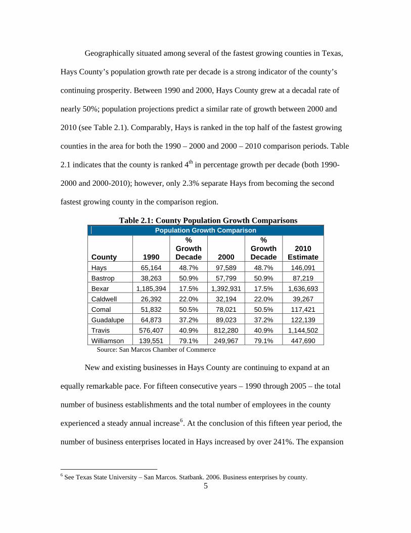
Geographically situated among several of the fastest growing counties in Texas,

Hays County’s population growth rate per decade is a strong indicator of the county’s

continuing prosperity. Between 1990 and 2000, Hays County grew at a decadal rate of

nearly 50%; population projections predict a similar rate of growth between 2000 and

2010 (see Table 2.1). Comparably, Hays is ranked in the top half of the fastest growing

counties in the area for both the 1990 – 2000 and 2000 – 2010 comparison periods. Table

2.1 indicates that the county is ranked 4th in percentage growth per decade (both 1990-

2000 and 2000-2010); however, only 2.3% separate Hays from becoming the second

fastest growing county in the comparison region.

Table 2.1: County Population Growth Comparisons

Source: San Marcos Chamber of Commerce

Population Growth Comparison

County 1990

% Growth Decade 2000

% Growth Decade

2010 Estimate

Hays 65,164 48.7% 97,589 48.7% 146,091 Bastrop 38,263 50.9% 57,799 50.9% 87,219 Bexar 1,185,394 17.5% 1,392,931 17.5% 1,636,693 Caldwell 26,392 22.0% 32,194 22.0% 39,267 Comal 51,832 50.5% 78,021 50.5% 117,421 Guadalupe 64,873 37.2% 89,023 37.2% 122,139 Travis 576,407 40.9% 812,280 40.9% 1,144,502 Williamson 139,551 79.1% 249,967 79.1% 447,690

New and existing businesses in Hays County are continuing to expand at an

equally remarkable pace. For fifteen consecutive years – 1990 through 2005 – the total

number of business establishments and the total number of employees in the county

experienced a steady annual increase6. At the conclusion of this fifteen year period, the

number of business enterprises located in Hays increased by over 241%. The expansion

5

6 See Texas State University – San Marcos. Statbank. 2006. Business enterprises by county.

of business enterprises has also had a positive effect on the total number of privately

employed persons (see Table 2.2). In 1990, the U.S. Census Bureau estimated that there

were approximately 11,300 privately employed persons in the county; that figure has

nearly tripled to 31,4667 in 2005.

Table 2.2: Charting the Business Development in Hays County: 1990 – 2005

Source: Statbank: Business Enterprises by County An analysis of the top 25 major private and public employers in Hays County for

2005 shows a diverse assortment of business enterprises and municipal entities. The top

employer in Hays County for 2005 was Texas State University – San Marcos with 6,406

employees; followed by the Prime and Tanger Outlet Centers with a combined employee

base of 3,540 (see Table 2.3). With a total labor force of 66,5508, the top three public and

private employers for the area constitute virtually 15% of the total local employment.

7 The employment figure 31,466 represents the total private nonfarm employment estimate. For additional information, see City of San Marcos. Economic Development San Marcos. 2006. San Marcos: demographic profile – 2006.

6

8 See City of San Marcos. Economic Development San Marcos. 2006. San Marcos: demographic profile – 2006.

7

Table 2.3: Hays County’s Top 25 Major Private and Public Employers - 2005 Major Hays County Employers - 2005

Rank Employer Number of Employees

1 Texas State University - San Marcos 6,406 2 Prime Outlets - San Marcos 2,000 3 Tanger Factory Outlet Center 1,540

4 San Marcos Consolidated Independent School District 1,081

5 Grande Communications 850 6 Hays County 802 7 Hunter Industries 650 8 Central Texas Medical Center 580 9 Gary Jobs Corps Center 567 10 HEB Distribution Center 540 11 City of San Marcos 465 12 Wal-Mart Super Center 435 13 Wide-Lite Corporation 325 14 San Marcos Treatment Center 284 15 C-FAN 276 16 Community Action Inc. 260 17 Chartwells 250 18 Heldenfels Enterprises, Inc. 227 19 Butler Manufacturing 220 20 Goodrich Aerostructures Group 200 21 McCoy Corporation 198 22 Thermon Manufacturing 177 23 Sac N Pac Stores, Inc. 147 24 San Marcos Baptist Academy 130 25 TXI Hunter Cement 130

Source: Economic Development San Marcos

The dynamic population growth and continuing business development within

Hays County is characteristic of the rapid development occurring throughout this

particular region of the state. However, there are distinguishing features in Hays County

that are responsible for a significant portion of the county’s economic and social

development. One of these distinctive characteristics is city of San Marcos.

San Marcos: The County Seat

Centrally located between the Austin MSA9 and the San Antonio MSA, the city

of San Marcos has considerably benefited from Hays County’s geographic position.

Situated only 26 miles from Austin and 45 miles from San Antonio, San Marcos’ ideal

locale is where 35% or roughly 50,000 of the county’s total population reside10. As the

county seat, San Marcos commands the county’s largest municipal operating budget at

$136, 419,25211 for the 2008 fiscal year.

Figure 2.2: Establishing a Regional Setting

8

Source: City of San Marcos: Planning and Development Services Department

9 As defined by the U.S. Census Bureau, a Metropolitan Statistical Area (MSA) is a geographic population cluster of more than 50,000 residents in a single city or consists of an urban area with more than 100,000 residents and includes each affected county. 10 The population estimates used to calculate this figure are located at the Texas Association of Counties. The County Information Project. 2007. Hays County profile. 11 See City of San Marcos. 2007. City of San Marcos: 2007-08 Annual Budget.

9

San Marcos’ rapid economic expansion has substantial ties to the retail and

tourism enterprises located in the area. As a cornerstone of fiscal development, the Prime

and Tanger Outlet Centers have been a foundation of the economic prosperity in San

Marcos. Mayor Susan Narvaiz recently made the observation that the city had become

“the third most popular tourist destination in Texas due to the success of our outlet malls”

(Millecam 2007, 2). San Marcos Today (2004, 35) further detail the success of the retail

and tourist attraction:

The development of two factory outlet retail centers in the city has had a strong impact on retail sales and tourism in San Marcos. Prime Outlets and the Tanger Outlet Center have a combined total of over 200 outlet stores. The centers employ approximately 2,800 persons. According to the Greater San Marcos Economic Development Council, the outlet malls attracted over 6 million shoppers in 2002. Since the vast majority of customers come from outside San Marcos, these facilities are similar to tourist attractions in terms of their economic impact. Since the publication of this article, the total number of employees for the outlet

centers has increased to 3,540 in Dec. 200512. Building on these economic achievements,

a large-scale operation is currently underway to construct a $21 million city conference

center and a $50 million Embassy Suite Hotel in close proximity to downtown San

Marcos. Both the conference center and the full-service hotel are slated to open in Oct.

2008 and expectations are that the two projects will further bolster the tourism and retail

industries for the area.

San Marcos Today (2004, 35) identifies two important factor contributing to the

dramatic increase in size and prosperity; the article makes the observation that the “large

population increase is attributable to (both) growth pressures from the Austin and San

Antonio metro areas and the large enrollment increases at Texas State University.”

12 See City of San Marcos. Economic Development San Marcos. 2006. San Marcos: demographic profile – 2006.

10

Texas State University – San Marcos

Texas State University – San Marcos (TSU) has also played an especially vital

role in the growth of the city and the county. As the largest university in the Texas State

University System13, TSU dominates the San Marcos landscape with a 457 acre main

campus and has over 5,000 additional acres of farm, ranch, residential, and recreational

space14. According to an excerpt by the San Marcos Planning and Development Services

Department (San Marcos Today 2004, 35):

Texas State University–San Marcos (formerly Southwest Texas State University), has a current enrollment of approximately 23,500 and a campus of over 300 acres. It is the sixth largest public university in the state and the largest employer in San Marcos. Texas State has expanded its educational offerings to include more than 114 undergraduate, 81 master's, and 5 doctoral degree programs. Texas State directly employs approximately 2,600 people. Due to its size in relation to the rest of San Marcos, the university has a large impact on the economy of the city and surrounding area. TSU’s student population has increased by 17% – to almost 28,000 – in the three

years since the publication of the San Marcos Today article; since then the university has

had to dramatically enlarge the number of faculty and staff on campus (Millecam 2007,

1). In Dec. 2005, TSU was the leading public employer in the county – an estimated

6,406 persons were employed by the university during that year15. Additional data

analysis reveals that the number of faculty at the university is currently estimated to be

1,27216. The steady annual increase in TSU students, faculty, and staff has provided San

13 The Texas State University System includes Texas State University at San Marcos, Lamar University at Beaumont, Sul Ross State University at Alpine, Sam Houston State University at Huntsville, and Angelo State University at San Angelo. 14 See Texas State University System. Texas State University – San Marcos. 2007. Texas State University profile. 15 See City of San Marcos. Economic Development San Marcos. 2006. San Marcos: demographic profile – 2006. 16 See Texas State University System. Texas State University – San Marcos. 2007. Texas State University profile.

11

Marcos with a reliable consumer base and educated labor market that supports their

burgeoning tourist and retail industries.

An analysis of the growth of TSU, San Marcos, and Hays County shows that the

three entities are experiencing similar rates of development (see Table 2.4). Between

1950 – 2000, Hays County grew at an average of 22% each decade. Comparatively, San

Marcos experienced an average decadal growth rate of 18%, while TSU experienced

decadal gains of 28% for the same time period. Remarkably, newly released population

forecasts project Hays County to exceed 173,000 residents in 2010, 279,000 in 2020,

417,000 in 2030 and 584,000 in 2040; these figures far outstrip previous county growth

rates and represent an estimated 499.1% increase in total population from 2000 to 204017

(see table 2.4). In the near future, Table 2.4 indicates that the city of San Marcos is

expected to more than double its total population by 2020 to 279,228. Although this

research does not specifically propose a correlation in the rates of growth between Hays

County, TSU, and San Marcos, the projected rapid expansion of one entity will invariably

have dramatic consequences on the growth of the other two.

Table 2.4: Population Growth Projections

Population Area 1950 1960 1970 1980 1990 2000 2005

2010 estimate

2020 estimate

2030 estimate

2040 estimate

Hays County 17,840 19,934 27,642 40,954 65,614 97,589 126,250 173,377¹ 279,228¹ 417,590¹ 584,642¹ City of San Marcos 9,980 12,713 18,860 23,420 28,743 34,733 46,112 53,457 71,841 96,548 n/a

Texas State University – San Marcos 2,013 2,653 9,852 15,400 20,940 23,556 27,500 n/a n/a n/a n/a

Source: City of San Marcos: Planning and Development Services Department ¹ - Texas State Data Center and Office of the State Demographer

17 See Texas State Data Center and Office of the State Demographer.

12

Interstate Highway 35: Linking Business Development and Community Growth

The enormous growth pressures and commerce activity generated by the Austin-

San Antonio corridor cannot be fully realized without taking into account the major

thoroughfare that connects them – Interstate Highway 35 (IH 35). According to the

Austin-San Antonio Intermunicipal Commuter Rail District (ASA Rail), the volume of

traffic on IH 35 has reached an all time high with “almost three million people in Central

Texas, traveling daily between Georgetown and San Antonio” (Financial and economic

benefits study 2007, 1). U.S. involvement in NAFTA18 contributes significantly to the

volume of daily commuters traveling through the area on IH 35 since the roadway

provides a vertical passageway between Mexico, Canada, and the U.S. According to the

Greater Austin-San Antonio Corridor Council:

80% of all Mexican exports pass through the Lone Star State, 75% of those exports traveling up Interstate 35 through Austin and San Antonio. Trade between Mexico and the United States has doubled to more than $100 billion in the last five years, and will double again by the year 2000. Nearly half of America's foreign exchange with Mexico involves products originating in or destined for Texas, and this explosion of trade presents ever-increasing opportunities for businesses throughout the Corridor19.

The regional population explosion is occurring at such a rapid rate that “the

Federal Highway Administration (FHWA) estimates that the current six lanes of IH-35

would need to be expanded to 12 to 18 lanes to accommodate expected population

growth in the Austin-San Antonio region by the year 2025” (Financial and economic

benefits study 2007, 7). Given the obvious economic implications of the Austin-San

Antonio corridor via IH 35, cities located near the roadway – such as Buda, Kyle, and

18 The North American Free Trade Agreement (NAFTA) is a trading bloc of nations which includes the United States, Mexico, and Canada. The primary goal of NAFTA is to increase trade by phasing out and eventually eliminating tariffs between the three North American trading partners. 19 See the Greater Austin-San Antonio Corridor Council homepage at http://www.thecorridor.org/history.html.

13

San Marcos – rely on competent local leadership to advance their community’s economic

profile using comprehensive methods of analysis.

Managing the Growth

Clearly, as the local population and economy continue to grow in complexity and

size, the need for Hays County to understand their economy using reliable

methodological tools to provide decision-making guidance has become greater. Lacking

the proper methods to monitor and regulate the progress of the regional economy, local

policymakers face an “extremely difficult task to promote industrial growth or to preserve

existing economic development” (Dake 1985, 10). Further exacerbating problems of local

economic development, a community’s dependence on relatively few industry types

make it exceedingly vulnerable to national economic fluctuations. Hence, it is important

that the regional economy be frequently monitored and properly diversified because

“without economic growth and a system to manage it, all of the other functions of public

administration” suffer (Rodriguez, 11).

Given its prime location, rapidly growing population, and economic growth

potential, the importance of identifying and encouraging key segments of Hays County’s

economy cannot be overstated. Economic development models provide a comprehensive

method for understanding the local economy and its strengths and weaknesses. Therefore,

it is the intention of this research project to examine the local economic structure of Hays

County, Texas using two distinct economic development models – the economic base

analysis (EBA) and shift-share analysis (SSA).

14

Economic Development Models: A Synopsis

Applying the economic base analysis20 and shift-share analysis consistently can

generate data capable of assisting local government officials understand the industrial

makeup of their local economy, control the rate of economic growth, forecast local and

national industrial trends, and interpret the fiscal impact of current decisions on future

growth. Briefly, an EBA allows researchers to classify an industry within a local

economy according to its import-export trade activities. An EBA places particular

emphasis on the export sector of an economy because it is theorized that export activities

are the engine of a local market. Export industries represent the economic base of an

economy and are responsible for attracting outside sources of revenue for the community.

Thus, the EBA allows analysts to determine which industries are “driving” the local

economy by identifying industries that export goods and/or services. On the other hand,

the SSA allows researchers to comparatively analyze local and national trends to

determine their differences across a fixed period of time.

Shift-share analysis is very practical in assessing the impacts of industrial restructuring on regional and local economies and for providing guidance for industrial targeting, and hence can make a significant contribution to understanding and selection of key leading industries in the region, which can help forming local industry partnerships (Dinc 2004, 4). In addition to explaining the existing local economic environment, the EBA and

SSA models allow public administrators to shape the local economy using informed

economic development policies. Deliberate growth policies and actions are more likely to

translate into controllable fiscal growth patterns; in turn, this allows local government

20 The literature also refers to the EBA as a comprehensive economic survey, economic base survey, economic survey, input-output approach, and regional export base study.

15

officials to draw from a reliably strong tax base, adeptly manage public goods and service

initiatives, and better plan for capital improvement projects.

In rapidly expanding locations, such as Hays County, it is important to have a

comprehensive economic development plan to maximize the local community’s

economic influence. Uncontrolled economic growth or decline is troublesome for a

community because of the various problems associated with major booms and rapid

declines (Galambos and Schreiber 1978). For example, rapid unstable economic growth

could potentially result in overcrowded public institutions, i.e. jails, hospitals, etc.

Overcrowded public facilities require the local government to make immediate

infrastructure expenditures to return the effected public institutions back to equilibrium.

The resulting debt incurred by the local government leaves the entire community

vulnerable to economic fluctuations. A significant disruption in a community’s tax base

can result in the loss of potential tax revenue and a rise in economic welfare assistance

programs demanded by an increasingly impoverished proportion of the community. EBA

and SSA models give policy makers a set of reliable tools capable of guiding their

decision-making process.

Despite some limitations within the EBA and SSA models (these will be

discussed at length in future chapters), the techniques are widely used analytical tools that

assist decision-makers to understand their communities’ local economy, protect against

the effects of uncontrolled growth and stagnation21, and maximize a community’s input-

output ratio to achieve optimal economic development conditions.

21 See Dake (1985, 8) for additional information regarding the diversification and stability of the regional economic base.

16

Chapter Summary

This chapter presents a rationale for studying Hays County’s local economy. The

rapid economic development combined with the large scale population growth has made

the county one of the fastest growing regions in the U.S. The need to protect and guide

the local economy according to effective economic policies has never been greater. Near

the conclusion of chapter two, a pair of economic development models – the economic

base study and shift-share analysis – are introduced as analytical methods to manage the

economic growth in the region. Using these techniques, public officials can maintain a

working knowledge of how their local economy is structured and operates. The next

chapter examines literature pertinent to the function and utility of the economic base and

shift-share models. Finally, the following chapter concludes with the construction of a

conceptual framework table.

17

Chapter III. Literature Review Chapter Overview

This chapter provides a synopsis of previous research that examines the value and

applicability of the economic base study (EBA) and shift-share analysis (SSA). In

particular, this literature review emphasizes the research conducted by Galambos and

Schreiber, Dinc, and Hustedde et al. To conclude the chapter, this research constructs a

conceptual framework table based on the literature that is later used to perform an

assessment of the economic health of Hays County, Texas.

Economic Growth: A Government’s Responsibility

In their article, “Economic Base Studies in Resource Administration”, Paul

Barkley and Thaine Allison, Jr. (1968) contend that the entire regional economic

structure is rapidly evolving and growing in complexity. Therefore, it is essential that

local officials have effective techniques to determine the cause, rate, and stability of their

area’s economic growth. In his applied research project, Jesus Rodriguez (1987, 8) re-

affirms that “in order to resolve problems of economic growth, local governments devise

(economic development) strategies to address defined issues” and, by doing so, they

insulate themselves from many unforeseen circumstances. Thus, as a result of avoiding

unexpected economic turmoil by using economic development models, policy makers

create a healthier economic environment for the entire local population.

According to the article “Regional and Local Economic Analysis Tools” by

Mustafa Dinc (2002, 3):

The ultimate goal of local and regional policy makers is to improve the well-being of the local population and promote opportunity and equity for them, which is possible only by increasing the competitive edge of their respective

18

regions. To do so, local and regional policy makers need to develop sound policies, and closely monitor the outcomes of these policies.

To combat the complexity of the regional economic structure and address the

need for analytical tools to interpret a local economy, the literature proposes a number of

economic growth models. The available techniques include “economic base studies, shift-

share analyses, input-output and labor supply or migration studies (all of which) have

gained their popularity in one form or another in terms of theoretical development and to

a lesser extent, in empirical analysis” (Liu 1974, 297). These models vary in

measurement, precision, prognostication accuracy, and simplicity; however, the intent of

each method is to guide policy makers in answering fundamental questions about their

area. For example, “what are the current economic conditions in the community? What

components of the community have been growing or what components have been

declining? What are the community’s options for improving its economic future and

which of those options should be pursued first?” (Hustedde et al. 2005, 1). By gaining a

better understanding of the current economic environment, policy makers can more

accurately predict their local community’s future financial health in an objective and

systematic manner.

As previously mentioned, there are a variety of existing techniques to analyze an

economy; however, two of the most well-known economic development models are the

economic base analysis (EBA) and the shift-share analysis (SSA). The EBA and SSA are

“models, (that) due to their simple and user friendly structures, are widely used by local

and regional development practitioners in industrial targeting, economic impact analysis,

and regional comparison across the world” (Dinc 2002, 4). Lending further credence to

the success of the EBA and SSA models is that they have a reliable reputation of

19

producing dependable data when consistently performed using the same data sets (Dake,

1985).

Economic Base Analysis: An Introduction

The classification of local industries into import and export categories is the basis

for the technique known as the economic base analysis. In their book, Making Sense Out

of Dollars: Economic Analysis for Local Government, Arthur Galambos and Eva

Schreiber (1978, 5) explain why segregating a local economy according to import and

export activities is an important feature of the model:

A good way to start diagnosing the health of the local economy is with an economic base study. Such a study is a systematic way of looking at each job in your local area and classifying it in one of two ways: Is it an export job [a job that produces goods and services sold mainly outside the local area], or is it a non-export job, whose output is consumed locally? The export job results in money from outside the area being pumped into the local economy through wages and business income. Throughout the literature, several direct and indirect industry classification

techniques are identified; these techniques are used to designate an industry as import or

export oriented. Despite the precision that direct methods typically offer, Galambos and

Schreiber (1978) ardently argue against the use of these methods due to their intensive

time, labor, and financial requirements. As a way to avoid these research boundaries,

Dinc (2005) proposes using the most commonly applied indirect method of industrial

classification - the location quotient.

Indirect Industry Classification: The Location Quotient

The location quotient (LQ) is a popular indirect method of identifying export

industries because it is easily applied and interpreting the results requires little expertise.

Fundamentally, the LQ measurement assesses “the extent to which total export

employment is spread among various industries and whether the economic base is

20

becoming more diversified over time or more widely spread among industries”

(Galambos and Schreiber 1978, 20). Location quotients are calculated for each industry

to determine if the local economy has a greater proportion of each industry than the

national economy. Thus, the location quotient can reasonably determine which industries

are comparatively exporting their goods and service and the extent of their involvement

in “driving” the local economy.

Another function of the LQ is that it can be used comparatively against the LQ of

another region of similar size and structure. For example, if region B is robustly

exporting goods and services in a specific sector and region A is aware of the

circumstances via the LQ, then region A can adjust its economic strategy accordingly.

Region A can choose to select an alternate industry type to encourage or local officials

can adopt an approach that aggressively challenges region B’s dominance in that sector.

In either scenario, using the location quotient to assess the strengths and weaknesses of

surrounding communities provides policy makers with a competitive advantage in

determining which direction the local economy should move.

The location quotient’s inferences are based on employment data gathered from

County Business Patterns (CBP) published by the United States Census Bureau.

Although the location quotient can be used in conjunction with a variety of other

community data – i.e. population, income, input/output variables, etc. – employment

figures from CBP are the most popular because of their accessibility. Both local and

national employment statistics are available through CBP to the general public in a user

friendly format. The basis for CBP’s employment data comes from calculating employers

quarterly payroll tax returns. Since employment data is retrieved in this fashion, CBP

21

does not include a small number of employee categories. These omitted categories

include: 1) government employees, 2) agricultural laborers, 3) entrepreneurs, and 4)

domestic service laborers. The literature asserts that the LQ results are reliable, but

cautions against using the conclusions of the study literally.

Once the LQ is determined using CBP data, the export employment multiplier

(EEM) can be calculated to examine the total economic impact of various decisions.

Specifically, the EEM is an estimate of the total employment attributable to changes in

the local export employment (Galambos and Schreiber 1978). Since export industries

create additional employment opportunities by generating new sources of revenue, the

multiplier estimates how many import jobs are created by the addition of one export job.

This estimate can be extrapolated to determine the total economic impact of export

employment changes in an industry. Lane (1966, 346) comments that the EEM can be “a

powerful tool for analyzing and forecasting economic activity,” if properly used in

conjunction with other techniques.

Economic Base Analysis: Clarifying the Export & Import Sectors

Since economic base analyses rely on distinguishing and classifying industries

according to their economic activities, it is important to make the distinction between

export22 and import23 industries. In his article, Sirkin (1959, 426) concludes that the total

economic output of a region can be divided into two sectors – “output and productive

services sold outside the area (i.e. exports) and output absorbed internally (i.e. imports).”

Noticeably, the distinguishing factor between the two sectors is whether an industry’s

goods and services are consumed locally or outside the region.

22 The literature also uses the terms base and/or basic industries to identify export industries. 23 The literature also uses the terms non-base or non-basic industries to identify import industries.

22

Export industries are the most important sector of a local economy because they

represent economic activities that generate additional revenue for the community. As a

result, a community is reliant on the export base to “produce spendable income for use by

the local economy” and to create new employment opportunities for the community by

increasing the region’s total economic output (Dake 1985, 16). The export base creates

“more jobs and income in the community than is found at the site of the new employer”

because of the increased consumption level of the import sector via the export sector

(Hustedde et al. 2005, 11). Since the import sector relies directly on the achievements of

the export base, the growth of export industries directly affects total economic growth. A

variety of consequences can result from decline of the export base, i.e. employment

stagnation, weak economic growth, or high levels of industrial concentration.

Import industries are “the economic complement of the base – namely, the service

enterprises” of a local market whose goods and services are consumed locally (Thomas

1964). Andrews (1953, 161) elaborates further:

Service enterprises include enterprises whose principal function is that of providing for the needs of persons within the community’s economic limits. They are also distinguished from the base in the fact that they are, principally, importers, or if they do not import, do not export their finished goods or services.

Hultman (1967, 151) lessens the importance of the import sector because “a

region develops largely around the export base which, according to some versions,

becomes the critical autonomous variable in determining the level of regional income.”

Yet, despite its diminished importance in export base research, Galambos and Schreiber

(1978, 23) offer a rare perspective on the role of imports, seldom discussed throughout

the literature.

Attempts to increase local employment in industrial categories that show imports can be just as effective in stimulating growth. Thus, local economic development

23

strategy should not concern itself strictly with increasing export employment to the exclusion of reducing imports. As mentioned above, a significant of portion of EBA literature neglects

the importance of import industries. Some research suggests that this is true

because researchers have been unable to establish a precise causal relationship

between the import and export sectors (Thomas, 1964). Although the export base

theory has yet to calculate the import sector as an absolute function of the total

output, it is presumed that when the “existence of the non-export sector of the

region’s commercial economy is completely dependent on the export sector,” then

the predictive value of the EBA model will have substantially increased (Thomas

1964, 428).

Direct vs. Indirect Industry Classification

The most direct method to determine the export/import categorization of a local

industry is to “conduct market surveys of all employers, or of a carefully selected sample,

through personal interviews with employers or mail questionnaires” (Galambos and

Schreiber 1978, 15). However, Galamobs and Schreiber (1978) conclude that contacting

every individual employer in a community is too costly and time intensive to be given

any serious consideration. Alternatively, Hustedde, Shaffer, and Pulver (2005) suggest

using direct observation to gauge whether or not an employer’s primary economic

activity is export oriented. Unfortunately, in many cases, the size and complexity of the

surrounding community make the direct observation technique nearly impossible. The

direct observation method is also viewed with skepticism as it is prone to higher levels of

researcher error and bias (Dinc, 2002).

24

Given the considerable limitations of directly identifying export industries,

researchers have largely turned their attention to indirect methods of classification. Dinc

(2002) identifies three popular indirect methods: 1) the minimum requirements technique;

2) differential multipliers: multiple regression analysis and 3) the location quotient

technique. Multiple regression analysis is not typically used to determine export

employment because of its limited flexibility and demanding time requirements. The

minimum requirements technique is seldom utilized because it has a “very specific

selection criteria for comparison areas” that can be restrictive (Dinc 2002, 23). Due to

their applicability and simplicity, “location quotients are frequently used as the indirect

method for classifying export and non-export employment” (Galambos and Schreiber

1978, 16). Se-Hark Park (1965, 384) cautions that whichever “method (is) used to divide

industry employment into export and local employment,” the results will vary according

to the applied method.

County Business Patterns

The economic base analysis and shift-share analysis utilize the same data source

and the same data variable to analyze the local economy. Typically, the techniques

examine employment data rather than other variables, i.e. population, income, output, etc.

Frequently, this is because employment statistics are easily obtained and come from a

reliable source – the United States Census Bureau24. Hustedde, Shaffer, and Pulver

(2005) identify a variety of the resources for local and national employment information:

• United States Census Bureau • County Business Patterns • Census Of Business • United States Bureau of Labor Statistics

24 The EBA and SSA models are worldly renowned for their simple and user-friendly data requirements; this is especially true in many developing countries where data is limited or unavailable.

25

Of these data sources, the most commonly used to perform regional analyses is

County Business Patterns (CBP). CBP is an annual publication issued by the U.S. Census

Bureau and includes local and national employment data that is calculated every March.

CBP arranges local employment estimates by county and U.S. employment figures

display the total national employment. Regional and national employment statistics are

organized according to the U.S. Census Bureau’s economic classification system – the

North American Industrial Classification System (NAICS). Although the literature

references the Standard Industrial Classification (SIC) system, modern adaptations to the

classification structure have produced NAICS25. NAICS contains more statistical detail

than SIC and accounts for various economic activities conducted by the U.S. with

Mexico and Canada that were previously disregarded.

Despite the level of detail and availability in CBP, there are two important

limitations that apply to this data set and, consequently, affect both models. First, County

Business Patterns is typically published two to three years later than the current date. The

lack of current data is a hindrance to the validity of an analysis because of the increasing

complexity and speed of a globalized economy. Although CBP provides large quantities

of reliable data, the statistics do not account for present phenomena. Secondly, CBP does

not take into consideration certain categories of employees. As previously discussed,

these employees include government workers, entrepreneurs, agricultural laborers, and

domestic service laborers. The oversight of this data occurs because employment

statistics are taken from quarterly payroll tax returns sent by employers. Although these

limitations are notable, EBA and SSA conclusions from CBP still maintain a solid

25 For additional information on SIC, please visit the U.S. Census Bureau at http://www.census.gov/epcd/www/naics.html.

26

reputation and are reliable if consistently performed to maintain the local economy and

are used as advisory tools.

Export Employment Multiplier

Walter Isard (1960, 190) defines the export employment multiplier (EEM) as the

ratio of “total employment in both basic and service activities divided by total basic

employment." The EEM is an important mathematical expression that indicates the effect

of local export employment over total local employment. The relevance of the export

employment multiplier exists in its predictive ability to indicate the consequences on the

total local economy of local export employment fluctuations. This indicator gives policy

makers a general impression of the impact that export employment growth or decline

would have on the economy as a whole. Although this calculation can be made for a

single year’s worth of data, Galambos and Schreiber (1978) note the narrow scope of this

type of measurement and caution against its use. Instead, they recommend researchers

obtain a more complete picture of the economic situation by comparing the EEM’s over

several years. Analyzing the EEM in this manner allows policy makers to draw

conclusions from data that is not representative of the true level of economic activity.

Despite the usefulness of the EBA and its various measurements, the method

provides no basis for comparing the local economy against national trends. By

supplementing the EBA with the shift-share technique, this issue is specifically

addressed.

Shift-Share Analysis: A Brief Literary Overview

Complementing the EBA, the shift-share analysis (SSA) is another trusted and

renowned economic development model. The SSA is “designed to interpret a region’s

27

growth in terms of the dynamics of its industrial structure by decomposing differences

between the value of a chosen variable as observed regionally and nationally” (Buck

1970, 445). Simply put, a shift-share analysis concentrates on local employment

fluctuations over a specific period of time and compares them against national

employment trends. Similarly, the shift-share analysis can use a variety of economic

variables to perform the study; however, employment data is most often used. The local

and national employment data used to perform the analysis in this research also originates

from County Business Patterns.

Shift-share analysis deconstructs a regional economy into three primary

components – national growth, industrial mix, and competitive share. The summation of

these three components is equal to the total economic change of the area. Dinc (2005, 4)

explains:

Shift-share analysis can give a description of total economic change that is attributable to the growth of the national economy, the industrial mix of the region, and the competitiveness of the local industries. By interpreting the results of the shift-share analysis, it is possible to explore the advantages of the local area, as well as to identify growth, or potential growth industries that are worthy of further investigation.

National Growth Component

The first step in conducting a shift-share analysis is to calculate the national

growth component (NG). NG measures the hypothetical share of regional job growth

attributable to growth of the national economy. Dinc (2002, 4) further remarks that the

“national share component measures the regional economic change that could have

occurred if the region had grown at the same rate as the reference area, and generally

refers to the national economy.”

28

Industrial Mix Component

The next step in computing the SSA is to calculate the industrial mix component

(IM). This measurement appraises the quantity of growth that can be attributed to the

regions mix of industries. As such, it is a helpful indicator in determining if the

community has large quantities of rapidly expanding industries or vice versa. According

to Hustedde, Shaffer, and Pulver (2005, 35):

The industrial mix component is determined by multiplying the local employment in each economic sector by the difference in the national growth rate for that sector and the growth rate for the whole economy. A positive industrial mix rate indicates the majority of local employment is in sectors growing faster national total employment negative industrial mix indicates just the opposite.

Competitive Share Component

The final component of SSA is the competitive share indicator (CS). The

competitive share component is often viewed by researchers as the most important of the

three because it is the only SSA variable which can be directly influenced by the local

population. The CS component measures the growth (decline) in an industry locally and

nationally; the resulting figure represents the region’s competitiveness for that industry.

This measurement is calculated by “multiplying the local employment in each economic

sector by the difference in the growth rate of that sector nationally and locally” (Hustedde

et al. 2005, 36).

Component Summation

The total economic change component (TEC) indicates an area’s actual growth or

decline and can be expressed as the sum of the three derivatives – the competitive share,

industrial mix, and national growth components (Houston, 1967).

29

Although the SSA is useful in illuminating certain aspects of a local economy, the

technique does not specify the reasons for the actual growth or decline in an area. Instead

local officials are responsible for diagnosing the reasons for changes using the SSA in

conjunction with other techniques. Hustedde, Shaffer, and Pulver (2005, 38) comment

that although the results of the SSA do not yield a one size fits all solution, policy makers

commonly select from a variety of solutions based on SSA results:

• Strengthen management capacities of existing firms through educational programs (personnel, finance, organization, etc.)

• Encourage business growth through identification of capital sources: o Loans (S.B.A., banks, industrial revenue bonding). o Equity (small business investment corporations, investment groups).

• Increase knowledge of new technology through educational programs in science and engineering.

• Aid employers in improving work force quality through educational programs, employment counseling and social services (e.g., day care, health services)

The results of the economic base study and shift-share analysis provide basic

information about the local economic structure that can be used as “a prime ingredient for

an effective local development strategy” (Galambos and Schreiber 1978, 3). Given that

the national economy is largely beyond the control of local policy makers, it is important

that local officials maintain a high degree of control over their own local economy

(Rodriguez 1987). Guidance provided by EBA and SSA conclusions allows informed

policy makers to have a greater degree of control over their community’s economic

growth strategy. Hence, “if done properly and routinely, the economic base analysis (and

shift-share analysis) will reveal trends which then can be effectively turned into strategies

designed to stabilize and encourage the economic base” (Dake 1985, 18).

Conceptual Framework: Overview

This research project utilizes the operations research method to provide a

framework for evaluating Hays County’s economy. Specifically, the operations research

30

models – the economic base analysis and the shift-share analysis – are the conceptual

framework used to conduct the examination.

Economic Base Study: Conceptual Framework

Considering the finite amount of resources that a local economy has at its

disposal, policy makers must make informed decisions to benefit the entire community.

By interpreting the results of an export base analysis, policy makers can best use “scarce

resources (tax dollars and other sources of revenue) to produce the most benefits, so that

constituents and taxpayers will be relatively well satisfied next they go to the polls”

(Galambos and Schreiber, 3). The literature emphasizes various scenarios which can

occur as a result of incompetent or inaccurate economic forecasting techniques; i.e. the

assumption of large amounts of local debt within a small period, turbulent economic

periods incongruent with national trends, etc. Shields (1998, 218) characterizes models of

operations research as a set of “complex techniques (which) are predictive by nature.”

Operations research models – such as the EBA - provide decision makers with user

friendly techniques to protect the community against misguided economic policies.

The first step in performing an export base analysis is to identify the components

and variables associated with the model. Table 3.1 identifies three EBA components – the

location quotient, the export employment estimate, and the export employment

multiplier. These components help give the technique substance and validity. The four

variables used to calculate the EBA components are identified in the table below as

various local and national employment statistics. Table 3.1a augments the conceptual

framework table by organizing the components and variables into mathematical

expressions.

31

Table 3.1: Conceptual Framework of an Economic Base Analysis Conceptual Framework Table Research Purpose: To analyze Hays County, TX to determine which industries generate economic growth and which industries demonstrate economic growth potential Components of an EBA: Scholarly Support: (X) Export Employment (LQ) Location Quotient (M) Export Employment Multiplier (E) Total National Employment (Ei) Total National Industry Employment (e) Total Local Employment (ei) Total Local Industry Employment

Dake (1985), Di Matteo (1993), Dinc (2002), Galambos and Schreiber (1978), Guccione and Gillen (1980), Linnemann (1985), Rodriguez (1987), Sirkin (1959)

Table 3.1a: Economic Base Analysis Equations

Equations for the EBA Conceptual Framework Table

LQ = ei / e ÷ Ei / E X = [ei / Ei - e / E] * Ei M = ei / X

Once the conceptual framework table is organized, the next step is to identify

what industries are present in the local economy. A local economy’s industries can be

located in County Business Patterns. Once the local employment data is located for the

regional economy using the six digit NAICS code, its national counterpart can be found

using the same code. For example, using CBP, hypothetical Industry Q would be listed as

an industry in Hays County, with a pre-assigned NAICS code26 and a total local industry

employment figure (ei). Once the NAICS code has been identified for hypothetical

Industry Q locally, the national employment figures are used to determine the total

national industrial employment (Ei). In Table 3.2, Example City has a local industry

employment figure of 900 workers and the total local employment figure for this city is

3,700. Comparatively, the total national industry figure for hypothetical Industry Q is

26 For the sake of simplicity, the NAICS code has been omitted in this example; however, it will be discussed more thoroughly in the next chapter.

32

4,000; the total national employment for the U.S. is 19,000. For the sake of brevity, the

figures in this example have been dramatically scaled down.

Table 3.2: Example – Identifying Local and National Employment Estimates

Area Industry Q Employment

Total Employment

Location Quotient (LQ)

Export Employment (X)

Export Employment Multiplier (M)

Example City 900 (ei) 3,700 (e) United States 4,000 (Ei) 19,000 (E)

Once this employment data is recorded, the researcher can then employ the

location quotient to identify export industries in the local economy.

Location Quotient Equation

As previously discussed, the location quotient is an indirect method of identifying

export industries. The location quotient is the ratio of total local industry employment to

total local employment divided by the ratio of total national industry employment to total

national employment. For any industry, if the resulting LQ is larger than 1, then that

industry contributes to the export base. If the LQ is equal to one, then it is assumed that

the industry produces only enough goods and services for local consumption. Therefore,

it would be categorized as a non-basic industry. If the resulting location quotient is less

than 1, then that industry is assumed to import its goods or not produce enough to sell

externally and is also classified as a non-basic industry. contributes to the import base.

Mathematically, the equation can be expressed as:

LQ = ei / e ÷ Ei / E

33

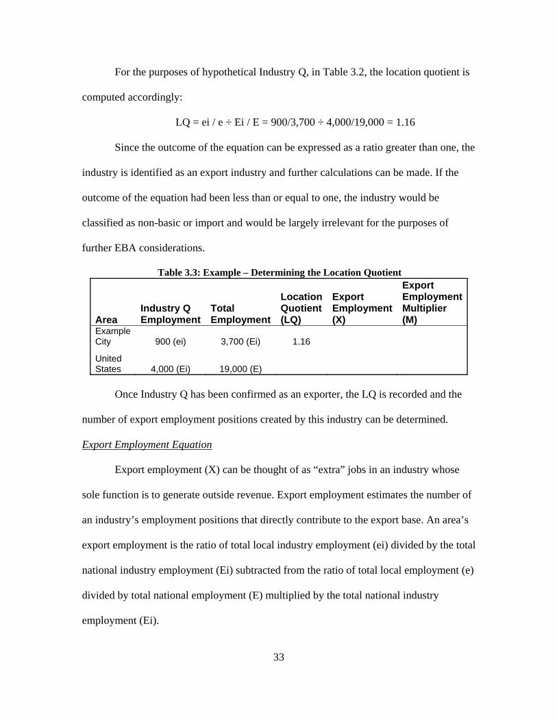
For the purposes of hypothetical Industry Q, in Table 3.2, the location quotient is

computed accordingly:

LQ = ei / e ÷ Ei / E = 900/3,700 ÷ 4,000/19,000 = 1.16 Since the outcome of the equation can be expressed as a ratio greater than one, the

industry is identified as an export industry and further calculations can be made. If the

outcome of the equation had been less than or equal to one, the industry would be

classified as non-basic or import and would be largely irrelevant for the purposes of

further EBA considerations.

Table 3.3: Example – Determining the Location Quotient

Area Industry Q Employment

Total Employment

Location Quotient (LQ)

Export Employment (X)

Export Employment Multiplier (M)

Example City 900 (ei) 3,700 (Ei) 1.16

United States 4,000 (Ei) 19,000 (E)

Once Industry Q has been confirmed as an exporter, the LQ is recorded and the

number of export employment positions created by this industry can be determined.

Export Employment Equation Export employment (X) can be thought of as “extra” jobs in an industry whose

sole function is to generate outside revenue. Export employment estimates the number of

an industry’s employment positions that directly contribute to the export base. An area’s

export employment is the ratio of total local industry employment (ei) divided by the total

national industry employment (Ei) subtracted from the ratio of total local employment (e)

divided by total national employment (E) multiplied by the total national industry

employment (Ei).

34

The export employment formula is expressed as:

X = [ei / Ei - e / E] * Ei

For the purposes of calculating the estimated export employment contribution

made by hypothetical Industry Q, the equation is:

X = [ei / Ei - e / E] * Ei = [900/4,000 – 3,700/19,000] * 4,000 = 121 Table 3.4: Example – Calculating the Number of Export Employment Positions

Area Industry Q Employment

Total Employment

Location Quotient (LQ)

Export Employment (X)

Export Employment Multiplier (M)

Example City 900 (ei) 3,700 (e) 1.16 121 United States 4,000 (Ei) 19,000 (E)

In other words, 121 of the 900 employees at Industry Q are contributing directly

to the export base.

Export Employment Multiplier Equation The third and final EBA component is the export employment multiplier, also

referred to as the regional base multiplier. According to the literature, the export

employment multiplier helps to “estimate local basic sector employment and allows

analysts to project non-basic sector job creation given an increase in basic sector

employment” (Dinc 2002, 15). The EEM is helpful in predicting the impact of

fluctuations in the export base on the total local economy. The EEM is the total local

industry employment (ei) divided by total export employment (X). The resulting figure

reflects the total number of jobs created in return for each new export employment

position. The EEM equation is:

M = ei / X

35

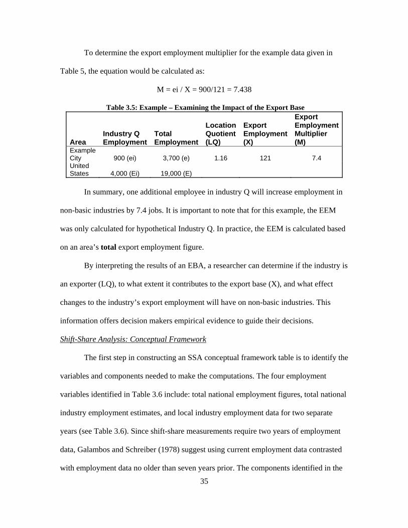
To determine the export employment multiplier for the example data given in

Table 5, the equation would be calculated as:

M = ei / X = 900/121 = 7.438

Table 3.5: Example – Examining the Impact of the Export Base

Area Industry Q Employment

Total Employment

Location Quotient (LQ)

Export Employment (X)

Export Employment Multiplier (M)

Example City 900 (ei) 3,700 (e) 1.16 121 7.4 United States 4,000 (Ei) 19,000 (E)

In summary, one additional employee in industry Q will increase employment in

non-basic industries by 7.4 jobs. It is important to note that for this example, the EEM

was only calculated for hypothetical Industry Q. In practice, the EEM is calculated based

on an area’s total export employment figure.

By interpreting the results of an EBA, a researcher can determine if the industry is

an exporter (LQ), to what extent it contributes to the export base (X), and what effect

changes to the industry’s export employment will have on non-basic industries. This

information offers decision makers empirical evidence to guide their decisions.

Shift-Share Analysis: Conceptual Framework

The first step in constructing an SSA conceptual framework table is to identify the

variables and components needed to make the computations. The four employment

variables identified in Table 3.6 include: total national employment figures, total national

industry employment estimates, and local industry employment data for two separate

years (see Table 3.6). Since shift-share measurements require two years of employment

data, Galambos and Schreiber (1978) suggest using current employment data contrasted

with employment data no older than seven years prior. The components identified in the

36

conceptual framework table are the national growth, competitive share, industrial mix,

and total economic change components. Based on the suggestion from Galambos and

Schreiber (1978), this research uses employment data 2005 and 1998.

Once all relevant local and national employment statistics are assembled using the

conceptual framework table, the process of determining the national growth, industrial

mix, and competitive share components can proceed. “When added together, the three

parts equal the total change in employment” and the shift and shares analysis can be

completed (Galambos and Schreiber 1978, 27). Table 3.6a supplements the SSA

conceptual framework table and provides the formulas needed to complete the analysis.

Table 3.6: Conceptual Framework Table of Shift-Share Analysis

Conceptual Framework Table Research Purpose: To analyze the local economy of Hays County, Texas so as to analyze the relative growth rate of the region against the national growth trend, measure industry diversification and its effect on the surrounding community, and examine regional industry growth as compared to national industry growth. Components of SSA: Scholarly Support: (Ei) Regional employment in a given industry at the beginning of a period (Ei*) Regional employment in a given industry at the end of a period (USi) National employment in a given industry at the beginning of the period (USi*) National employment in a given industry at the end of the period (US) Total national employment at the beginning of a period (US*) Total national employment at the end of the period (NG) National Growth (IM) Industrial Mix (CS) Competitive Share (TEC) Total Economic Change

Dake (1985), Di Matteo (1993), Dinc (2002), Galambos and Schreiber (1978), Houston (1967), Linnemann (1985), Seyfried (1996)

37

Table 3.6a: Shift and Share Analysis Equations

Equations for the Conceptual Framework Table

NG = Ei (US* / US – 1)

IM = Ei (USi* / USi – US* / US)

CS = Ei (Ei* / Ei – USi* / USi) TEC = NG + IM + CS

Shift-Share Components: NG, IM, CS, & TEC

The national growth (NG) component is used to calculate a local industry’s

growth rate as compared to the total national economy. As illustrated above in Table

3.6a, the national growth component is expressed as:

NG = Ei (US* / US – 1)

The industrial mix (IM) component is used to determine the extent to which

individual local industries factor into the growth or decline of the local economy as a

whole. The industrial mix formula is:

IM = Ei (USi* / USi – US* / US) Finally, the competitive share (CS) component of the shift-share analysis

estimates how well or poorly an industry has performed versus its national counterparts.

This equation is expressed as:

CS = Ei (Ei* / Ei – USi* / USi)

The total economic change (TEC) is equivalent to the total employment change in

the region; this estimate is relatively simple to compute. The equation is:

TEC = NG + IM + CS

38

The shift-share analysis is a multi-faceted series of techniques designed to

supplement the export base study. The SSA strengthens the EBA by providing the

analysis with a reference point, i.e. the U.S. economy, to compare the local economy

against.

Chapter Summary

Scholarly works such as Rodriguez (1987), Galambos and Schreiber (1978), Dake

(1985), and Hustedde, Shaffer, and Pulver (2002) are excellent literary sources that

identify the utility and practicality of economic development models. The economic base

and shift-share results can be further strengthened if data is collected and processed

routinely. Barkley and Allsion (1968, 473) caution that if only a snapshot of time is

taken, then the conclusions suffer from being “static and represent the structure of a local

economy only at one point in time.” In spite of these limitations, there is a “growing

appreciation of the magnitude of the problems urban communities face” and the need to

effectively address these issues (Murdock 1962, 69). Thus, models of operations research

– such as the EBA and SSA – are needed to assist policy makers. The components and

variables identified in the literature and recorded in the conceptual framework tables

demonstrate how policy makers can begin to operationalize these methods.

Chapter IV. Methodology

Chapter Overview The purpose of this chapter is to describe the data collection methods used to

analyze the local economy of Hays County, Texas. The chapter also operationalizes the

39

conceptual framework table presented in the previous chapter. Finally, this chapter

discusses the limitations of conducting an economic base study and shift-share analysis.

North American Industrial Classification System

This research uses aggregate data analysis to determine the level of export

employment spread throughout various industries in Hays County, the extent of industrial

diversification in the region, and compare local and national economic trends. To

accomplish these objectives, local and national employment statistics are collected from

the annual publication County Business Patterns (CBP). Released by the U.S. Census

Bureau, CBP typically lags two to three years behind real-time economic activities. The

publication provides employment data that support comprehensive industry analysis for

both local and nationwide examination purposes.

Prior to 1997, economic statistics were categorized according to the Standard

Industrial Classification (SIC) system. However, due to the growing complexity of the

international economic environment and the need for more precise methods of

measurement, the Census Bureau adopted the North American Industrial Classification

System (NAICS) in 1997. Developed in cooperation with Mexico and Canada, the

NAICS established a North American business classification system and allows for more

congruent data comparison between the three trading partners. As opposed to the 9

industrial categories associated with the SIC system, the NAICS has 20 international

industrial classification categories.

The NAICS categorizes industries according to a predetermined six-digit industrial

code which allows for a greater amount of precision as compared to the four-digit SIC

index. In 2002, the NAICS codes underwent a partial revision and the changes were

40

reflected in the 2003 County Business Patterns publication. According to the U.S. Census

Bureau, fourteen of the twenty sectors were completely unaffected by the restructuring

process and only two sectors – Wholesale Trade and Construction – were overhauled

substantially27. Briefly, the Census Bureau defines the six-digit North American

Industrial Classification System accordingly:

• The 1st and 2nd digits represent a sector of the economy; this is the broadest level

of the categorization.

• The 3rd digit signifies a sub-sector.

• The 4th digit represents an industry group.

• The 5th digit designates a particular industry. This digit is the most precise of the

national industrial classification codes.

• The 6th and final digit is used to classify industries according to national origin,

i.e. Canada, Mexico, or the United States.

An example of the NAICS classification process is illustrated in Table 4.1. As

demonstrated below, the categorization of manufactured goods becomes more refined

with the inclusion of an additional digit.

Table 4.1: Example – North American Industrial Classification System

27 The 2002 NAICS revision process affected six sector categories: Construction, Wholesale Trade, Information, Retail Trade, Mining, and Administrative Support, Waste Management, & Remediation Services. For additional information, visit the United States Census Bureau – North American Industrial Classification System (NAICS) webpage at http://www.census.gov/naics/2007/index.html.

NAICS Code Description

31---- Manufacturing

313 Textile Mills: Fiber, Yarn, and Thread

3131 Mills: Fiber, Yarn, and Thread

31311 Mills

313111

Yarn Spinning Mills: Yarn Texturizing, Throwing, and Twisting

Although CBP yields reliable aggregate data, there are various limitations to the

precision of the NAICS employment statistics. First, there is a substantial delay in data

reporting by the County Business Patterns. The tremendous volume of information

collected by the Census Bureau typically takes two to three years to process and release

to the general public. In a rapidly changing global marketplace, a two to three year data

lag can present a misleading or inaccurate economic profile of a community. Secondly,

CBP fails to include employment data for government workers, agricultural laborers, and

domestic homemakers. Since CBP derives its data from an employers’ payroll tax return,

it fails to include any worker not reported using this method. This limitation can be

mitigated if the analyses are augmented with employment data from other sources.

Despite these minor limitations, CBP remains the most trusted method of indirect data

collection and analysis; this is particularly true because CBP is not overly resource

intensive and it provides a reasonably accurate economic profile.

Economic Base Study: Operationalization Table

For this research project, the unit of analysis is employment data published in

County Business Patterns. By manipulating the employment statistics using the formulas

and techniques located in the literature, this research can operationalize the conceptual

framework table proposed at the conclusion of Chapter III. The four variables and three

41

42

components that constitute the EBA are located below in Table 4.2; also included in the

table are the methods this research uses to generate the measurements from the

employment data.

Table 4.2: Operationalization of the EBA Conceptual Framework Table

Operationalization Table Components of an EBA: Measurement: (E) Total National Employment (Ei) Total National Industry Employment

(e) Total Local Employment

(ei) Total Local Industry Employment

Employment figures based on estimates derived from U.S. Census Bureau Data, County Business Patterns

(LQ) Location Quotient LQ =ei / e ÷ Ei / E

(X) Export Employment X = [ei / Ei - e / E] * Ei

(M) Export Employment Multiplier M = e / X Shift-Share Analysis: Operationalization Table

This research also conducts a shift-share analysis using employment data gathered

from County Business Patterns across a period of five years – 2000 and 2005. By

manipulating these employment statistics using selected formulas located the shift-share

conceptual framework table is operationalized – see Table 4.3.

Table 4.3: Operationalization of the SSA Conceptual Framework Table

43

Operationalization of Conceptual Framework Table Components of SSA: Measurement: (Ei) Regional employment in a given Industry at the beginning of a period (Ei*) Regional employment in a given industry at the end of a period (USi) National employment in a given industry at the beginning of a period (USi*) National employment in a given industry at the end of the period (US) Total national employment at the beginning of a period

(US*) Total national employment at the end of the period

Estimates based on figures derived from U.S. Census Bureau Data, County Business Patterns

(NG) National Growth NG = Ei (US* / US – 1) (IM) Industrial Mix IM = Ei (USi* / USi – US* / US) (CS) Competitive Share CS = Ei (Ei* / Ei – USi* / USi) (TEC) Total Economic Change TEC = NG + IM + CS

Methodological Considerations

Economic development techniques, such as the EBA and SSA, are proven

analytical tools; however, there are a few considerations that should be taken into account

when these methods are used for analysis.

• First, these models make broad generalizations about a local economy and its

industrial infrastructure. Hence, it is important that the results from the analyses

should be used to inform and provide direction to policymakers and are not

intended for explicit functions.

• Next, conclusions drawn from the models can be bolstered over time if enough

data is collected and processed routinely to provide a method of comparison

across time. If only an economic snapshot is taken, the conclusions risk being

“static and (may) represent the structure of a local economy only at one point in

time” (Barkley and Allison 1968, 473).

44

• Finally, the results from the economic growth models can be augmented by

utilizing sources of data to supplement County Business Pattern. Although some

methods may prove expensive in terms of time, money, and manpower, these

analyses should provide a richer picture of the local economy when used in

conjunction with the results of the EBA and SSA.

Economic Growth Models: Advantages

The literature cites critical advantages that the EBA and SSA models bring to

local economic analyses. First, these tools provide a logical method of examining local

economic data where none previously existed. Both models of operations research offer

“a practical analytical framework enabling researchers to gain an increased insight into

the functions of economic growth” (Thomas 1964, 424). Even Tiebout, who offers harsh

criticisms about the structure and function of the EBA and SSA models, cedes that it

offers up analysis of data in a meaningful way as compared to other competing

frameworks (Tiebout 1956). Given the significance of understanding the local economy,

the importance of objectively organizing and analyzing the fiscal health of a community

is an important priority.

Secondly, the structured framework provided by the EBA and SSA techniques

offers the user a simple and straightforward method to analyze a local market. The

simplicity and direct applicability of these models to any local economy around the world

has distinguished these techniques and made them extremely popular analytical tools.

The speed and simplicity of the models, however, do not always work to their advantage.

Murdock (1962, 68) observes that “as a quick, simple method (it) was an admittedly

crude instrument, but this was understood and accepted as the cost to be paid for the

45

speed and simplicity it embodied.” Although some critics decry the models as overly

simplistic at times, the need for local governments to quickly analyze their economies

and make informed decisions means that economic development models have an

important function in local government.

Economic Growth Models: Disadvantages

As is true for all methodologies, the literature identifies some inherent design

limitations within the economic base and shift-share models. First, Barkley and Allison

(1968) stress that the export base and shift-share method are static economic profiles of a

local market. The results generated from a single year’s analysis should be cautiously

used because they may not be representative of a community’s actual economic

development. By applying the methods to several different points in time, ranging from

five to seven years apart, the validity of the models dramatically increases (Thomas

1968). However, the SSA and EBA findings are not meant to prognosticate with absolute

precision, but rather offer a more profound impact as advisory tools for public

administrators (Galambos and Schreiber 1978). Performing the analyses competently and

consistently in this manner mitigates the severity of this limitation and allows for a more

accurate picture of the local economy.

Another disadvantage to the use of economic growth models is outlined in the

1964 article authored by Morgan Thomas. Thomas (1964, 429) points to several variables

that can cause industries in an economy to grow despite the conclusions from the models.

The list of external factors that can adversely affect the findings of EBA and SSA are as

follows:

1. If there is an injection of investment from the outside region sufficiently large enough to compensate for the contraction of exports, in a given region,

46

2. If the industries which obtain their resources and sell their products in the region grow sufficiently to compensate at least for the decline in exports, or

3. Through an improvement in the regions terms of trade with surrounding areas or the national markets.

Tiebout (1956) expands on these points by remarking that a typical regional

economy is comprised of hundreds of economic units which are all engaged in creating

wealth. Researchers have been unable, thus far, to precisely identify all of the variables

that account for the scenarios mentioned above. The increasing integration of the local

economy in the global marketplace has only exacerbated the number of unknown external

variables.

Lastly, local officials in cities with a high ratio of government employees, i.e.

Hays County, must be vigilant when using analyses of this type. The conclusions

generated from these methods fail to account for government employees and, depending

on the size of the workforce, will vary from the actual results. For example, Hays County

has several significant government employers – Texas State University – San Marcos,

San Marcos CISD, and Hays County – which are unaccounted for by employment

estimates in County Business Patterns. The absence of this data negatively affects the

value of these analyses; however, this inadequacy can be limited by using the EBA and

SSA techniques in conjunction with other economic analysis models to offer a

comprehensive view of the local economy.

Human Subjects Protection This applied research project used aggregate data analysis to address the research

topic and achieve its objectives. After a thorough review of exempt research categories

47

listed by the Institutional Review Board (IRB)28, this research project was found to be

exempt from IRB approval by 45 CFR, Part 46, Sec. 101(b), Item 429. Exemption status

was granted on the basis that only existing data sources were reviewed and no human

subjects were used throughout the course of this study.

Chapter Summary This chapter presented a methodological basis for performing the EBA and SSA

on Hays County’s economy. The chapter also discussed the utility of using CBP as a

reliable data source despite the exclusion of certain categories of workers. This chapter

concluded with a summation of the major strengths and weaknesses of the two techniques

as they are applied to a local economic structure. The next chapter discusses the results of

the application of the EBA and SSA models to the local economy of Hays County, Texas.

28 For additional information regarding IRB exempt categories please visit http://www.txstate.edu/research/irb/irb_exemption_categories.php. 29 For additional information regarding IRB statutes please visit http://edocket.access.gpo.gov/cfr_2002/octqtr/45cfr46.101.htm.

48

Chapter V. Results

Chapter Overview The purpose of this chapter is to review the results of the economic base analysis

(EBA) and the shift-share analysis (SSA) as applied to Hays County, Texas. The chapter

presents a sector analysis that identifies the largest industry exporters in the county. The

chapter also analyzes the county’s competitive share component against national trends.

Prior to examining the details of export employment or competitive shares, a broad

perspective of the local economy is given to summarize the findings. The complete list of

EBA and SSA data computations are found in Appendices A & B.

Economic Base Analysis: Summary of Results A total of 76 sub-sectors were identified in Hays County, TX as contributing to

the local economy (see Appendix A). Using the location quotient technique, 32 of the 76

sub-sectors were classified as export oriented. Summarizing the conclusions in Table 5.1,

this research identifies five sectors – Retail Trade, Health Care and Social Assistance,

Mining, Manufacturing, and Construction – with the greatest number of export industries.

These five sectors have a total of 25 export sub-sectors that represent 78% of the total

number export industries (see Table 5.1). Alternatively, the results of the analysis also

indicate that there are nine major NAICS sectors in Hays County lacking export oriented

industries. These industries include:

• Forestry, Fishing, Hunting, and Agriculture Support • Wholesale Trade • Finance and Insurance • Professional, Scientific, and Technical Services • Management of Companies and Enterprises • Admin., Support, Waste Mgmt., and Remediation Services • Educational Services • Arts, Entertainment, and Recreation • Unclassified Establishments

49

The remaining six categories have a varying combination of export and import

oriented industries.

Table 5.1: Twenty Major Business Sectors Contributing to the Hays County Export Economy

NAICS Code Sector Categories

Total # of Sub-Sectors Examined

Number of Export Industry

11---- Forestry, Fishing, Hunting, and Agriculture Support 1 0

21---- Mining 3 3 22---- Utilities 1 1 23---- Construction 3 3 31---- Manufacturing 18 7 42---- Wholesale Trade 3 0 44---- Retail Trade 12 9

48---- Transportation and Warehousing 6 1

51---- Information 5 1 52---- Finance and Insurance 3 0

53---- Real Estate, Rental, and Leasing 3 1

54---- Professional, Scientific, and Technical Services 1 0

55---- Management of Companies and Enterprises 1 0

56----

Admin., Support, Waste Mgmt., and Remediation Services 2 0

61---- Educational Services 1 0

62---- Health Care and Social Assistance 4 3

71---- Arts, Entertainment, and Recreation 3 0

72---- Accommodation and Food Services 2 1

81---- Other Services (except Public Administration) 3 2

99---- Unclassified Establishments 1 0 Sub-Sector Totals 76 32

Source: Appendix A * Italicized NAICS sector codes indicate top export oriented industries

50

Economic Base Analysis: Top Export Employers

Table 5.2 analyzes the top ten export employment contributors in Hays County.

The top three include Food Services and Drinking Places, Clothing and Clothing

Accessories Stores, and Social Assistance. Taken as a whole, these three industries

comprise 54% of Hays County’s total local export employment, while the top ten

combine to constitute 84% of the county’s total export employment.

Table 5.2: Top 10 Export Employment Sub-Sectors

Ranking NAICS Code Sub-sector

Local Employment

Percentage of Total Local Employment

Export Employment

1 722 Food Services and Drinking Places 4,427 14.1% 1,947

2 448 Clothing and Clothing Accessories Stores 2,357 7.5% 1,935

3 624 Social Assistance 1,000 – 2,499* 5.6% 1,121

4 237

Heavy and Civil Engineering Construction 871 2.8% 626

5 623 Nursing and Residential Care Facilities 1,412 4.5% 613

6 332 Fabricated Metal Product Manufacturing 859 2.7% 447

7 327 Nonmetallic Mineral Product Manufacturing 525 1.7% 399

8 335

Electrical Equipment, Appliance, and Component Manufacturing 250 - 499* 1.2% 259

9 493 Warehousing and Storage 250 - 499* 1.2% 218

10 441 Motor Vehicle and Parts Dealers 730 2.3% 205

TOTAL *For those employment estimates where no whole number was given, the mean was used to calculate the outcomes. 13,681 43.6% 7,770

Source: Appendix A

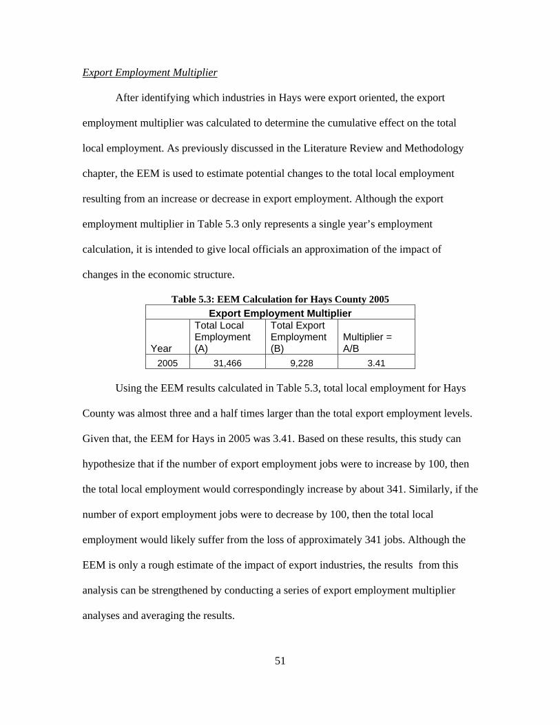
51

Export Employment Multiplier After identifying which industries in Hays were export oriented, the export

employment multiplier was calculated to determine the cumulative effect on the total

local employment. As previously discussed in the Literature Review and Methodology

chapter, the EEM is used to estimate potential changes to the total local employment

resulting from an increase or decrease in export employment. Although the export

employment multiplier in Table 5.3 only represents a single year’s employment

calculation, it is intended to give local officials an approximation of the impact of

changes in the economic structure.

Table 5.3: EEM Calculation for Hays County 2005 Export Employment Multiplier

Year

Total Local Employment (A)

Total Export Employment (B)

Multiplier = A/B

2005 31,466 9,228 3.41 Using the EEM results calculated in Table 5.3, total local employment for Hays

County was almost three and a half times larger than the total export employment levels.

Given that, the EEM for Hays in 2005 was 3.41. Based on these results, this study can

hypothesize that if the number of export employment jobs were to increase by 100, then

the total local employment would correspondingly increase by about 341. Similarly, if the

number of export employment jobs were to decrease by 100, then the total local

employment would likely suffer from the loss of approximately 341 jobs. Although the

EEM is only a rough estimate of the impact of export industries, the results from this

analysis can be strengthened by conducting a series of export employment multiplier

analyses and averaging the results.

52

Shift-Share Analysis: Summary of Results The SSA is comprised of three different components that measure a local

economy; the national growth, industrial mix, and the competitive share component. Of

these three measurements, the competitive share is the most important calculation

because it is the only component that can be directly affected by local policy makers.

Calculating the competitive share component routinely can help determine whether or not

the local economy is capturing its share of that industry as compared to the national

economy. If the result of the competitive share (CS) is positive, then the local economy is

capturing its market share of that industry. If the result of the competitive share is

negative, then the local economy is not capturing its full market share of that industry and

policy makers should look to improve the situation, especially if the industry has been

identified as an important exporter through export base analysis.

Tables 5.4 through 5.7 specifically address the competitive share component of

the Hays County shift-share analysis. Each table represents an aspect of the competitive

share component; this is useful for policy makers to understand because they

comparatively identify the strengths and weaknesses of the local economy with how the

national economy is performing. Prior to analyzing the results, it is important to re-iterate

that the results of the SSA tell the researcher what is occurring, it does not reveal why the

local economy is reacting in the way it has.

Table 5.4 is the most important table of the four addressing the CS component

because it alerts researchers to negative trends in the local economy. According to the

table, there are a total of nine industries that are losing their competitive share in the local

economy as compared to the nation. Electronics and Appliance Stores (NAICS Code

53

443) show the greatest amount of loss at -107 jobs. This reduction in CS represents over a

quarter of the county’s current total losses. Furthermore, the identification of this

industry, in particular, is important to note because it was previously identified by the

EBA results as one of the top ten exporters in the county. Again, although the reasons for

the decline in this industry are beyond the scope of the EBA and SSA, policy makers

should be urged to investigate further.

Table 5.4: CS – Expanding Nationally and Declining Locally

NAICS Code Description

Competitive Share (CS)*

442 Furniture and Home Furnishings Store -18

443 Electronics and Appliance Stores -107

488 Support Activities for Transportation -7

533

Lessors of Nonfinancial Intangible Assets (except Copyrighted Works) -1

561 Administrative and Support Services -38

562 Waste Management and Remediation Services -68

622 Hospitals -46

711 Performing Arts, Spectator Sports, and Related Industries -60

712 Museums, Historical Sites, and Similar Institutions -56

Total Competitive Share (CS) -401 Source: Appendix B

* Each competitive share component represents one employment position

54

Table 5.5 indicates that 26 sub-sectors and 2 sectors30 demonstrated a strong local

economic presence while simultaneously declining nationally. While some may assume

that this optimistic picture of the local economy should be cause for praise, this table

should be looked at with extreme prejudice. The industries listed in Table 5.5 are all

receding at the national level; since national growth is more likely to be an indicator of

local growth, the economic benefits currently experienced by the community may be

short lived. In other words, industries possessing a competitive share in a declining

national field may shortly be experiencing the same fate. On a positive note, the

industries listed in the table below have obviously been successful in improving their

economic standing in the community and local officials should take notice of that fact.

30 The shift-share analysis for 2000 and 2005 used two distinct NAICS code systems. Some of the codes for this study were incongruent, thus the study relied on two digit sector totals.

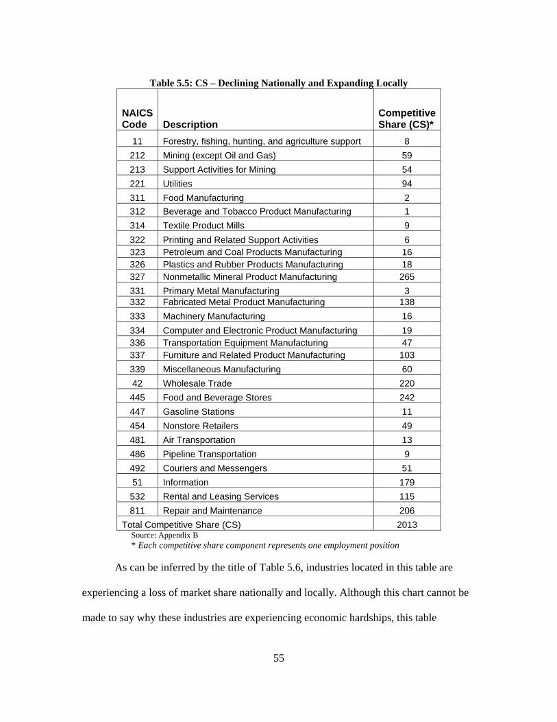
55

Table 5.5: CS – Declining Nationally and Expanding Locally

NAICS Code Description

Competitive Share (CS)*

11 Forestry, fishing, hunting, and agriculture support 8 212 Mining (except Oil and Gas) 59 213 Support Activities for Mining 54 221 Utilities 94 311 Food Manufacturing 2 312 Beverage and Tobacco Product Manufacturing 1 314 Textile Product Mills 9 322 Printing and Related Support Activities 6 323 Petroleum and Coal Products Manufacturing 16 326 Plastics and Rubber Products Manufacturing 18 327 Nonmetallic Mineral Product Manufacturing 265 331 Primary Metal Manufacturing 3 332 Fabricated Metal Product Manufacturing 138 333 Machinery Manufacturing 16 334 Computer and Electronic Product Manufacturing 19 336 Transportation Equipment Manufacturing 47 337 Furniture and Related Product Manufacturing 103 339 Miscellaneous Manufacturing 60 42 Wholesale Trade 220 445 Food and Beverage Stores 242 447 Gasoline Stations 11 454 Nonstore Retailers 49 481 Air Transportation 13 486 Pipeline Transportation 9 492 Couriers and Messengers 51 51 Information 179 532 Rental and Leasing Services 115 811 Repair and Maintenance 206

Total Competitive Share (CS) 2013 Source: Appendix B * Each competitive share component represents one employment position

As can be inferred by the title of Table 5.6, industries located in this table are

experiencing a loss of market share nationally and locally. Although this chart cannot be

made to say why these industries are experiencing economic hardships, this table

56

provides an excellent way for policy makers to determine which sub-sectors need direct

assistance from the local government.

Table 5.6: CS – Declining Nationally and Declining Locally

NAICS Code Description

Competitive Share (CS)*

321 Wood Product Manufacturing -103

324 Petroleum and Coal Products Manufacturing -103

325 Chemical Manufacturing -3

335

Electrical Equipment, Appliance, and Component Manufacturing -25

453 Miscellaneous Store Retailers -38

523

Securities, Commodity Contracts, and Other Financial Investments and Related Activities -12

551 Management of Companies and Enterprises -200

99 Unclassified establishments -7 Total Competitive Share (CS) -491

Source: Appendix B * Each competitive share component represents one employment position

Finally, Table 5.7 examines those local and national industries that are

experiencing synonymous growth. A number of industries in this table have large

competitive share values. Within these industries, in particular, policy makers can look

for clues and strategies on how to improve the standing’s of the rest of their local

industries. The expansion of these industries nationally is a powerful indicator that these

sub-sectors will continue to grow locally as well.

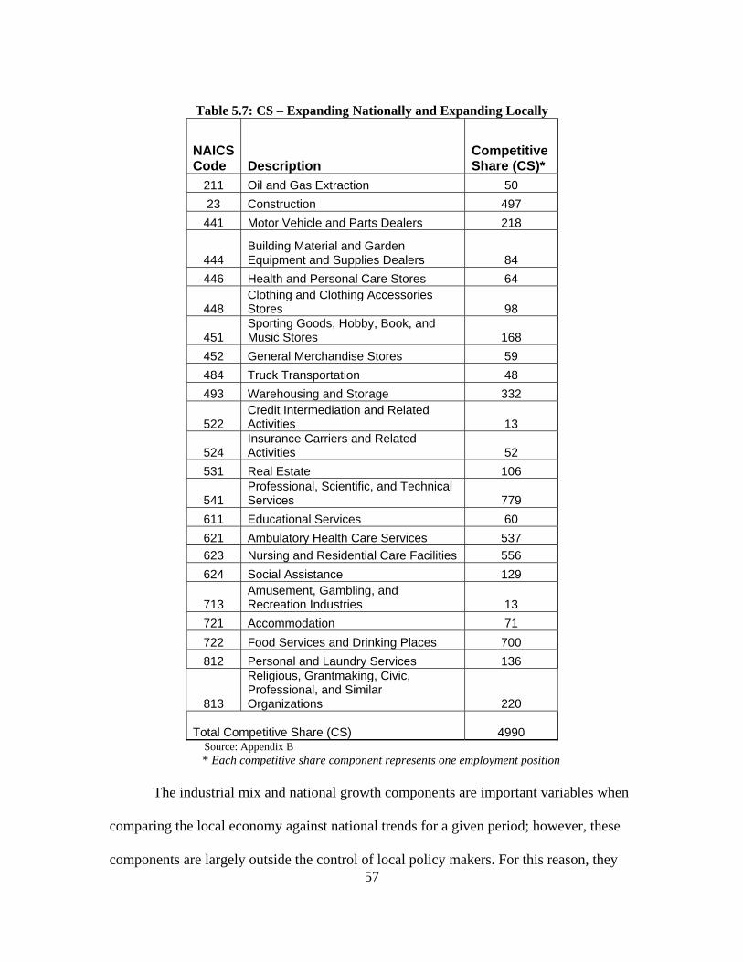
57

Table 5.7: CS – Expanding Nationally and Expanding Locally

NAICS Code Description

Competitive Share (CS)*

211 Oil and Gas Extraction 50 23 Construction 497 441 Motor Vehicle and Parts Dealers 218

444 Building Material and Garden Equipment and Supplies Dealers 84

446 Health and Personal Care Stores 64

448 Clothing and Clothing Accessories Stores 98

451 Sporting Goods, Hobby, Book, and Music Stores 168

452 General Merchandise Stores 59 484 Truck Transportation 48 493 Warehousing and Storage 332

522 Credit Intermediation and Related Activities 13

524 Insurance Carriers and Related Activities 52

531 Real Estate 106

541 Professional, Scientific, and Technical Services 779

611 Educational Services 60 621 Ambulatory Health Care Services 537 623 Nursing and Residential Care Facilities 556 624 Social Assistance 129

713 Amusement, Gambling, and Recreation Industries 13

721 Accommodation 71 722 Food Services and Drinking Places 700 812 Personal and Laundry Services 136

813

Religious, Grantmaking, Civic, Professional, and Similar Organizations 220

Total Competitive Share (CS) 4990

Source: Appendix B * Each competitive share component represents one employment position The industrial mix and national growth components are important variables when

comparing the local economy against national trends for a given period; however, these

components are largely outside the control of local policy makers. For this reason, they

58

are not as extensively reviewed by the results chapter of this research project as the

competitive share component is. However, the calculations and results of the industrial

mix and national growth components are included in Appendix B for further review.

Chapter Summary

This chapter analyzed the results of the economic base study and shift-share

analysis performed on Hays County 2005. The economic base analysis identified retail,

construction, and manufacturing industries as leading the way, economically speaking, in

Hays County. With regard to the results of the shift-share analysis, the element analyzed

for this method was the competitive share component because it is the only variable that

local policy makers have the ability to affect. The next chapter will offer concluding

thoughts and recommendations.

59

VI. Conclusion Chapter Overview This chapter briefly summarizes the findings of each chapter. Moreover, this

chapter offers recommendations on the practicality and usefulness of economic base

analysis and shift-share analysis for diagnosing a community’s financial health.

Summary of Chapters This research project is divided into five primary chapters. Chapter two examines

the economic progress Hays County has made via maintaining positive population trends,

a prosperous business atmosphere, and hypothesizes how the future growth of Hays

County might impact the region. Hays County’s rapid growth can be primarily attributed

to the Austin-San Antonio Corridor, Texas State University – San Marcos, and the

continued growth of the county seat, San Marcos. The Austin-San Antonio Corridor,

aided by NAFTA and made possible by IH 35, has provided the surrounding region with

a sustainable flow of outside revenue. The annual growth of TSU ensures the community

of an educated labor pool and consumer base. Finally, San Marcos’ geographic location

between two of the fastest growing metropolitans in the U.S. – Austin and San Antonio –

and within 200 miles of Dallas and Houston present the city with a number of

opportunities. Continual population growth in conjunction with steady employment

increases bodes well for the city at the present time. Finally, the chapter concludes with

the introduction of the economic base analysis (EBA) and the shift-share analysis as a

means to manage the rapid growth in the region.

Chapter three reviews literature pertinent to the discussion of the economic base

analysis and the shift-share analysis. By analyzing various literary sources, an indirect

60

industry classification technique – the location quotient – is selected to perform the

analysis on Hays County. Utilizing employment statistics located in County Business

Patterns, the literature identifies a reliable and user friendly data set. From the

methodological foundation documented in the literature, a conceptual framework table is

constructed to analyze Hays County’s local economy.

Chapter four introduces the reader to the methodology surrounding the export

base theory and shift-share technique. The chapter reviews the concept of the North

American Industrial classification System (NAICS) and how it functions within County

Business Patterns. The chapter builds upon the conceptual framework table constructed

in the previous chapter and provides direction on how the research aims to operationalize

the methods.

Finally, chapter five provides a summary of the results that occurred from the

application of the EBA and SSA to Hays County’s local economy. This chapter confirms

what many people had suspected, Hays County is a robust and diverse economy with

strong ties to the retail, construction, manufacturing, and health services industry groups.

An important revelation made by the SSA was that despite the national economic

slowdown occurring in manufacturing, the industry is experiencing significant growth in

Hays County. The relevance of this notion is that local economy’s typically have little

influence on their national counterparts; thus, if the manufacturing industries are failing

nationally, then a manufacturing slowdown may well be on the horizon for Hays County

as well.

61

Final Considerations EBA and SSA models are limited in the perspective they can provide policy

makers; however, these techniques can guide policy makers, assuming they are

consistently applied and the results are interpreted in the proper context. With regard to

Hays County, the research conclusions for the county have a limited impact because of

the large government sectors in the area. In particular, the exclusion of 6,406 TSU staff

and faculty, 1,081 San Marcos CISD employees, and 802 Hays County municipal

workers by County Business Patterns’ data set should caution policy makers against

accepting the conclusions of this study outright. The exclusion of this data this limits the

validity and accuracy of the EEM shown in Table 5.3.

Despite the effort of this research initiative to project absolute results, it takes

several years worth of analyses to have accurate measurements and consistent data to

draw true conclusions from. It would be naively incorrect to base any major decisions on

the results of this analysis alone. This further re-emphasizes the necessity of local

governments to perform analyses on a regular basis to monitor the fiscal health of the

community, so that they avoid relying solely on conclusions which might contain skewed

data. In spite of these limitations, this research demonstrates that in a period of national

prosperity, Hays County is flourishing and experiencing rapid growth of its own in an

increasingly diversified local economy. Whether the trend will continue can only be

determined by careful observation and informed action.

62

Bibliography Anderson, Sherry. 1999. A study to describe the opinions and attitudes on tax abatements

from county judges in Texas. Applied Research Project. http://ecommons.txstate.edu/arp/178/.

Andrews, Richard. 1953. Mechanics of the urban economic base: Historical development

of the base concept. Land Economics 29 (2): 161-167. Austin-San Antonio Intermunicipal Commuter Rail District. Financial and economic

benefits study. 2007. Austin, TX: U.S. http://asarail.org/resources/ASA_Rail_Economic_Study_Report-200703.pdf

Babbie, E. 2001. The practice of social research, 9th edition. Belmont: Wadsworth

Publishing/Thompson Learning Inc. Barkley, Paul, and Thaine Allison, Jr. 1968. Economic base studies in resource

administration. Land Economics. 44 (4): 470-479. Brown, A.J. and E.M. Burrows. 1977. Regional economic problems. London: George

Allen and Unwin Unlimited. Casler, Stephen. 1988. A theoretical context for shift and share analysis. Regional Studies

23 (1): 43-48. City of San Marcos. The San Marcos City Council. 2007. City of San Marcos: 2007–08

annual budget. http://www.ci.san-

marcos.tx.us/departments/finance/documents/AdoptedBudget08.pdf City of San Marcos. Economic Development San Marcos. 2006. San Marcos:

demographic profile – 2006. http://www.ecodevsanmarcos.org/SanMarcos_Profile.pdf City of San Marcos. Planning and Development Services Department. 2004. San Marcos

horizons: San Marcos today. http://www.ci.san-

marcos.tx.us/departments/planning/Docs/Horizons/San%20Marcos%20Today10.04.pdf

Dake, Bill. 1985. An economic base and shift and shares analysis for Bell County with

emphasis on Temple, Texas. San Marcos: Texas State University-San Marcos Press.

63

Di Matteo, Livio. 1993. Booming sector models, economic base analysis, and export-led economic development: Regional evidence from the Lakehead. Social Science History 17 (4): 593-617.

Dinc, Mustafa, and Kingsley Haynes. 1999. Sources of regional inefficiency: An

integrated shift-share, data envelopment analysis and input-output approach. The Annals of Regional Science. 33 (4): 469-489.

Farst, Debra. 2003. Perceptions toward downtown: Surveying city managers in smaller

Texas towns. Applied Research Project. http://ecommons.txstate.edu/arp/40/. Galambos, Eva, and Arthur Schreiber. 1978. Making sense out of dollars: economic

analysis for local government. Washington D.C.: National League of Cities. Garcia, Armando. 1991. An evaluation of the economic impact of the Sematech Research

Consortium on the economy of Austin, Texas. Applied Research Project. http://ecommons.txstate.edu/arp/234/.

Greenberg, Michael. Sports facilities and metropolitan economic development: The

impact of professional sports facilities on sales tax revenue in metropolitan statistical areas. Applied Research Project. http://ecommons.txstate.edu/arp/173/.

Guccione, A. and W.J. Gillen. 1980. Export-base and neoclassical type models of urban

growth: A synthesis. The Canadian Journal of Economics. 13 (4): 700-711. Haig, Robert. 1928. Major economic factors in the metropolitan growth and arrangement.

Regional Survey of New York City and Its Environs (1): 43. Hertzler, Latrice. 1990. Local industrial location selection issues: A study of

intergovernmental initiatives attracting new technology and industry to Texas for urban growth and development. Applied Research Project. http://ecommons.txstate.edu/arp/232/.

Houston, David. 1967. The shift and share analysis of regional growth: A critique.

Southern Economic Journal 33 (4): 577-581. Hultman, Charles. 1967. Exports and economic growth: A survey. Land Economics 43

(2): 148-157. Hustedde, Ronald, Shaffer, Ron, and Glen Pulver. 2005. Community economic analysis:

A how to manual. Ames: Iowa State University Printing Services. Isard, Walter. 1961. Methods of regional analysis: An introduction to regional science.

Geographical Review 51 (4): 593-594.

64

Kiser, Donald. 1992. A location quotient and shift-share analysis of regional economies

in Texas. Applied Research Project. http://ecommons.txstate.edu/arp/238/. Klosterman, Richard. 1990. Community and analysis planning techniques. Savage:

Rowmand and Littlefield Publishers, Inc. Krumme, Gunter. 1968. Werner Sombart and the economic base concept. Land

Economics 44 (1): 112-116. Lane, Theodore. 1966. The urban base multiplier: An evaluation of the state of the art.

Land Economics 42 (3): 339-347. Lester, Nina. 2005. Assessing economic development incentives: Central Texas City:

Managers perspectives. Applied research Project. http://ecommons.txstate.edu/arp/6/.

Linnemann, John. 1985. An economic base study and shift and shares analysis of Travis County, Texas. San Marcos: Texas State University-San Marcos Press.

Liu, Ben-Chieh. 1974. Economic base and economic structure growth: Quantitative and

qualitative measures. Land Economics 50 (3): 297-301. Matthews, Charles. 1999. The 1986 Tax Reform Act: Its impact, with special emphasis

on Texas cities. Applied Research Project. http://ecommons.txstate.edu/arp/120/.

McKethan, Kevin. 1997. A study to describe the attitudes and perceptions of Texas

municipal officials on the effectiveness of tax abatements and incentives. Applied Research Project. http://ecommons.txstate.edu/arp/196/.

McNulty, James. 1977. A test of the time dimension in economic base analysis. Land

Economics 53 (3): 359-368. Millecam, Melissa. 2007. City of San Marcos, Texas, and John Q. Hammons Hotels &

Resorts, LLC Break Ground on Embassy Suites® Hotel and Conference Center. City of San Marcos.

http://www.ci.san-marcos.tx.us/cityhall/citymanager/documents/GroundbreakingPR.pdf

Mulligan, Gordon, and Lay James Gibson. 1984. Regression estimates of economic base

multipliers for small communities. Economic Geography. 60 (3): 225-237.

65

Murdock, John. 1962. Homer Hoyt and the dilemma of urban economic base analysis: A reply. Land Economics 38 (1): 66-69.

North, Douglas. 1956. Exports and regional economic growth: A reply. The Journal of

Political Economy 64 (2): 165-168. Nussbaum, Frederick. 1933. A history of the economic institutions of modern Europe.

New York: F.S. Crofts & Co. O’Leary, Daniel. 1995. Municipal revenue sources for general fund expenditures: A

review of Texas cities. Applied Research Project. http://ecommons.txstate.edu/arp/98/.

Park, Se-Hark. 1965. The economic base identification: An appraisal. Land Economics

41 (4): 382-386. Parr, John. 1999. Regional economic development: An export stages framework. Land

Economics 75 (1): 94-114. Pearson, David. 2002. An explanatory study of rural hospital closures and their links to

the economic health of local communities. Applied Research Project. http://ecommons.txstate.edu/arp/55/. Rodriguez, Jesus. 1987. Local government strategies for managing economic growth: A

case study of Bexar County. San Marcos: Texas State University-San Marcos Press.

San Marcos Chamber of Commerce. San Marcos Chamber of Commerce: Area

Demographics. 2007. Population growth comparison: Austin-San Antonio Corridor, 1990-2010.

http://www.sanmarcostexas.com/4154095_13751.htm Seyfried, William. "Examining the economic competitiveness of the economies of the

southern United States." Shift-Share Analysis. http://www.westga.edu/bquest/1996/seyfried.html.

Schneider, Mark. 1992. Undermining the growth machine: The missing link between

local economic development and fiscal payoffs. The Journal of Politics 54 (1): 214-230.

Shields, Patricia. 1998. Pragmatism as philosophy of science: A tool for public

administration. Research in Public Administration 4: 195-225. Shofner, Suzan. 2000. The impacts of smart growth on municipal finance: Perspectives of

city planning directors across Texas. Applied Research Project. http://ecommons.txstate.edu/arp/155/.

66

Sirkin, Gerald. 1956. The theory of the regional economic base. The Review of Economic

41 (4): 426-429. Sombart, Werner. 1916. Der moderne kapitalismus. Berlin: Duncker & Humboldt. Stewart, Charles. 1959. Economic base dynamics. Land Economics 35 (4): 327-336. Talbert, Stacie. 1998. An analysis of the impact of convention centers on hotel occupancy

tax revenues in Texas cities. Applied Research Project. http://ecommons.txstate.edu/arp/145/.

Texas Association of Counties. The County Information Project. 2007. Hays County

profile. http://www.txcip.org/tac/census/profile.php?FIPS=48209 Texas State Data Center and Office of the State Demographer. The University of Texas at

San Antonio. 2006. Projections show rapid population growth, diversification, and aging, but also increasing disparities in the levels and distribution of growth if recent trends continue point to a Texas population that is growing rapidly, increasingly diverse and aging.

http://txsdc.utsa.edu/tpepp/2006projections/summary/ Texas State University – San Marcos. Statbank. 2006. Business enterprises by county. http://brs.newsbank.com.libproxy.txstate.edu/cgi-

bin/statbank/sbnkSEARCH.pl?CVV=Hays&p_d=SBNK&LOC=TEXAS&CAT=ECONOMY&TOP=BUSINESS+ENTERPRISES+BY+COUNTY%0D%0A&state=kdkap9.2.1&p_nb_id=H5FS4ESCMTE5NjI1NzIzNi45NjMwOTE6MToxMjoxNDcuMjYuMTEuODA&CVPASS=true

Texas State University System. Texas State University – San Marcos. 2007. Texas State

University profile. http://www.tsus.edu/institutions/TxSt_profile.html Thomas, Morgan. 1960. Economic activity in small areas. Land Economics 36 (2): 164-

171. Thomas, Morgan. 1964. The export base and development stages theories of regional

economic growth: An appraisal. Land Economics 40 (4): 421-432. Tiebout, Charles. 1956. The urban economic base reconsidered. Land Economics 32 (1):

95-99. United States Census Bureau. County Business Patterns. 2005. 2005 County Business

Patterns (NAICS): Hays, TX. U.S. Government Printing Office, Washington, DC: U.S.

67

United States Census Bureau. County Business Patterns. 2005. 2005 County Business

Patterns (NAICS): United States. U.S. Government Printing Office, Washington, DC: U.S.

United States Census Bureau. U.S. Census Bureau News. 2007. 50 fastest-growing metro

areas concentrated in the west and south. http://www.census.gov/Press-

Release/www/releases/archives/population/009865.html United States Census Bureau. U.S. Census Bureau News. 2007. Arizona’s Maricopa

County leads counties in population growth since census 2000. http://www.census.gov/Press-

Release/www/releases/archives/population/009756.html The World Bank. World Bank Institute. Public Finance, Decentralization and Poverty

Reduction Program. 2002. Regional and local economic analysis tools, by Mustafa Dinc. http://info.worldbank.org/etools/docs/library/128789/Dinc%202001.pdf

68

Appendix A

Appendix Purpose The purpose of Appendix A is to provide empirical data to support the

conclusions of the EBA portion of this research project. The data listed below has been

uniformly assembled and organized according to the column titles and NAICS

identification. Further elaboration on the construction and organization of this table is

outlined below.

Column Identification Identification and explanation of the columns in this spreadsheet:

I. The first two columns – (1) and (2) - express the North American Industrial

Classification System (NAICS) code used by County Business Patterns and give a

description of the industry code. For the purposes of this research, a three digit

NAICS code is used to conduct the economic base study. In brief, the six-digit

NAICS code can be defined accordingly:

• The 1st and 2nd digits identify an overall industry classification; this

represents the broadest level of classification.

• The 3rd digit signifies a sub-sector within a given industry. This digit is

the most used for general research purposes.

• The 4th digit denotes a given industry group.

• The 5th digit represents a specific industry; this digit is the most

precise indicator reflecting national industrial classification codes.

• The 6th and final digit is used to classify industries according to their

national origin, i.e. Canada, Mexico, or the United States.

69

II. Columns three (3) and four (4) provide specific industry employment figures for

the national economy in 2005 and the percentage each industry represents in the

total national economy. As of 2005, the total national employment figure for the

U.S. was 116,317,003.

III. The figures in column five (5) express the quantity of local employees per each

industry. Since some employment figures were presented as a range, the mean of

the two variables was used to make further calculations. Specifically, the

following employment ranges were averaged accordingly:

0 - 19 – employment mean used = 10 20 - 99 – employment mean used = 60 100 - 249 – employment mean used = 175 250 - 499 – employment mean used = 375 500 - 999 – employment mean used = 750 1,000 - 2,4999 – employment mean used = 1,750

IV. Column six (6) provides the local employment requirements for each NAICS

code and is determined by multiplying the percentage figure in column four by

31,466 – this represents the total local employment amount for Hays County in

2005.

V. The figures in column seven indicate either export or import employment figures.

Export/import employment statistics are used to determine the strengths and

weaknesses of the local economy, as well as the location quotient in column

eight.

VI. The LQ notations in column eight are determined by subtracting the Hays County

employment figure in column five from the local requirements in column 6

thereby generating a result which is > 1 <. If the difference between the two

columns is greater than one, then it indicates export employment for Hays County

70

and is represented in the table as a normal integer. If the difference between the

two columns is less than or equal to one, then it indicates import employment

Hays County and is represented in the table as red colored integer enclosed in

parentheses.

The national employment figures are provided by the County Business Patterns,

United States, 2005, published by the United States Census Bureau. Employment figures

for Hays County are provided by the County Business Patterns, Texas, 2005, also

published by the U.S. Census Bureau. The format for this export employment spreadsheet

is based a similar worksheet by Galambos and Schreiber (1978, 25).

71

Export Employment Worksheet: Hays County, TX - 2005

Export Employment computed from location quotients: Hays County, TX – 2005

(1) (2) (3) (4) (5) (6) (7) (8)

Employment Category U.S. Employment Hays County Employment

Hays County Employment

for Local Requirements

Excess Employment = Export or

(deficit) LQ Notation

NAICS Code Description Amount

% of Total Amount

(col. 4 times 31,466)

(col. 5 minus col. 6)

(col. 7 > 1 = Export)

***For non-specific employment figures, calculations were made using the mean*** Forestry, fishing, hunting, and agriculture support:

115

Support Activities for Agriculture and

Forestry 92,001 0.08% 1 25 (24) Mining:

211 Oil and Gas Extraction 86,562 0.07% 20 - 99 22 38 Export

212 Mining (except Oil

and Gas) 196,940 0.17% 20 - 99 53 7 Export

213 Support Activities for

Mining 96,261 0.08% 20 - 99 25 35 Export Utilities:

221 Utilities 633,106 0.54% 175 170 5 Export Construction:

236 Construction of Buildings 1,613,063 1.39% 441 437 4 Export

237

Heavy and Civil Engineering Construction 908,222 0.78% 871 245 626 Export

238 Specialty Trade Contractors 4,260,042 3.66% 1,284 1152 132 Export

Manufacturing: 311 Food Manufacturing 1,469,730 1.26% 170 396 (226)

312

Beverage and Tobacco Product Manufacturing 154,233 0.13% 0 - 19 41 (31)

314 Textile Product Mills 163,675 0.14% 0 - 19 44 (31)

321 Wood Product Manufacturing 555,942 0.48% 20 - 99 151 (92)

322 Paper Manufacturing 453,966 0.39% 100 - 249 123 52 Export

323 Printing and Related Support Activities 657,759 0.57% 91 179 (88)

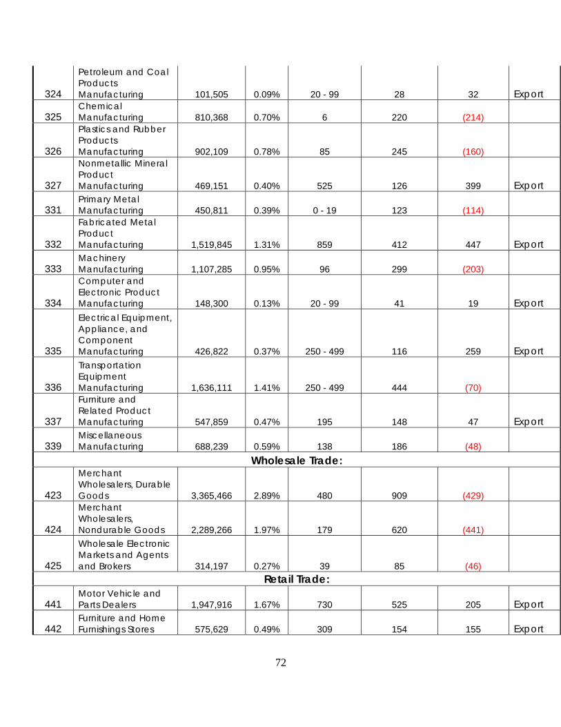
72

324

Petroleum and Coal Products Manufacturing 101,505 0.09% 20 - 99 28 32 Export

325 Chemical Manufacturing 810,368 0.70% 6 220 (214)

326

Plastics and Rubber Products Manufacturing 902,109 0.78% 85 245 (160)

327

Nonmetallic Mineral Product Manufacturing 469,151 0.40% 525 126 399 Export

331 Primary Metal Manufacturing 450,811 0.39% 0 - 19 123 (114)

332

Fabricated Metal Product Manufacturing 1,519,845 1.31% 859 412 447 Export

333 Machinery Manufacturing 1,107,285 0.95% 96 299 (203)

334

Computer and Electronic Product Manufacturing 148,300 0.13% 20 - 99 41 19 Export

335

Electrical Equipment, Appliance, and Component Manufacturing 426,822 0.37% 250 - 499 116 259 Export

336

Transportation Equipment Manufacturing 1,636,111 1.41% 250 - 499 444 (70)

337

Furniture and Related Product Manufacturing 547,859 0.47% 195 148 47 Export

339 Miscellaneous Manufacturing 688,239 0.59% 138 186 (48)

Wholesale Trade:

423

Merchant Wholesalers, Durable Goods 3,365,466 2.89% 480 909 (429)

424

Merchant Wholesalers, Nondurable Goods 2,289,266 1.97% 179 620 (441)

425

Wholesale Electronic Markets and Agents and Brokers 314,197 0.27% 39 85 (46)

Retail Trade:

441 Motor Vehicle and Parts Dealers 1,947,916 1.67% 730 525 205 Export

442 Furniture and Home Furnishings Stores 575,629 0.49% 309 154 155 Export

73

443 Electronics and Appliance Stores 469,248 0.40% 165 126 39 Export

444

Building Material and Garden Equipment and Supplies Dealers 1,262,662 1.09% 448 343 105 Export

445 Food and Beverage Stores 2,937,918 2.53% 914 796 118 Export

446 Health and Personal Care Stores 1,037,354 0.89% 247 280 (33)

447 Gasoline Stations 908,818 0.78% 364 245 119 Export

448

Clothing and Clothing Accessories Stores 1,555,928 1.34% 2357 422 1935 Export

451

Sporting Goods, Hobby, Book, and Music Stores 631,095 0.54% 280 170 110 Export

452 General Merchandise Stores 2,670,710 2.30% 651 724 (73)

453 Miscellaneous Store Retailers 819,903 0.70% 349 220 129 Export

454 Non-store Retailers 521,491 0.45% 113 142 (29) Transportation & Warehousing:

481 Air Transportation 486,355 0.42% 20 - 99 132 (73) 484 Truck Transportation 1,478,299 1.27% 168 400 (232)

486 Pipeline Transportation 148,674 0.13% 0 - 19 41 (32)

488 Support Activities for Transportation 543,666 0.47% 52 148 (96)

492 Couriers and Messengers 547,255 0.47% 20 - 99 148 (89)

493 Warehousing and Storage 578,040 0.50% 250 - 499 157 218 Export

Information:

511 Publishing Industries (except Internet) 1,032,273 0.89% 87 280 (193)

512

Motion Picture and Sound Recording Industries 314,396 0.27% 84 85 (1)

517 Telecommunications 1,226,536 1.05% 416 330 86 Export

518

Internet Service Providers, Web Search Portals, and Data Processing Services 452,159 0.39% 20 - 99 123 (64)

519 Other Information Services 54,052 0.05% 0 - 19 16 (7)

Finance and Insurance:

74

522

Credit Intermediation and Related Activities 3,201,715 2.75% 417 865 (448)

523

Securities, Commodity Contracts, and Other Financial Investments and Related Activities 860,384 0.74% 48 233 (185)

524

Insurance Carriers and Related Activities 2,323,045 2% 147 629 (482)

Real estate & rental & leasing: 531 Real Estate 1,480,040 1.27% 308 400 (92)

532 Rental and Leasing Services 634,901 0.55% 100 - 249 173 2 Export

533

Lessors of Nonfinancial Intangible Assets (except Copyrighted Works) 29,136 0.03% 0 - 19 9 1

Professional, scientific, & technical services:

541

Professional, Scientific, and Technical Services 7,689,366 6.61% 1,469 2080 (611)

Management of companies and enterprises:

551

Management of Companies and Enterprises 2,856,418 2.46% 344 774 (430)

Admin., support, waste mgt., remediation services:

561 Administrative and Support Services 8,946,939 7.69% 1,103 2420 (1317)

562

Waste Management and Remediation Services 333,343 0.29% 53 91 (38)

Educational services: 611 Educational Services 2,879,374 2.48% 476 780 (304)

Health care and social assistance:

621 Ambulatory Health Care Services 5,422,574 4.66% 1,549 1466 83 Export

622 Hospitals 5,321,600 4.58% 500 - 999 1441 (692)

623

Nursing and Residential Care Facilities 2,959,571 2.54% 1412 799 613 Export

624 Social Assistance 2,321,402 2% 1,000 - 2,499 629 1121 Export Arts, entertainment, & recreation:

75

711

Performing Arts, Spectator Sports, and Related Industries 412,146 0.35% 0 - 19 110 (101)

712

Museums, Historical Sites, and Similar Institutions 120,908 0.10% 0 - 19 31 (22)

713

Amusement, Gambling, and Recreation Industries 1,403,430 1.21% 212 381 (169)

Accommodation and food services: 721 Accommodation 1,854,499 1.59% 333 500 (167)

722 Food Services and Drinking Places 9,171,410 7.88% 4427 2480 1947 Export

Other services (except public administration):

811 Repair and Maintenance 1,294,783 1.11% 486 349 137 Export

812 Personal and Laundry Services 1,337,443 1.15% 360 362 (2)

813

Religious, Grantmaking, Civic, Professional, and Similar Organizations 2,758,728 2.37% 751 746 5 Export

Unclassified establishments:

99 Unclassified establishments 31,153 0.03% 4 9 (5)

TOTAL EMPLOYMENT 116,317,003 97.99% 31,466 30,829 9228

***For non-specific employment figures, calculations were made using the mean***

76

Appendix B

Appendix Purpose

The purpose of Appendix B is to provide empirical data to support the

conclusions of the SSA portion of this research project. The data listed below has been

uniformly assembled and organized according to the column titles and NAICS

identification. Further elaboration on the construction and organization of the table is

outlined below.

Column Identification Identification and explanation of the columns in this spreadsheet:

77

I. The first two columns – (1) and (2) - express the North American Industrial

Classification System (NAICS) code used by County Business Patterns and give a

description of the industry code. For the purposes of this research, two and three

digit NAICS codes were used to perform the shift-share analysis. A minor

variation in NAICS digits was necessary due to the unavailability of a small

number of three digit employment codes. There are four 2 digit NAICS categories

are 1) Forestry, fishing, hunting, and agriculture support; 2) Construction; 3)

Wholesale Trade; and 4) Information.

II. Columns three and four are representative of 2000 and 2005 national employment

figures and the corresponding percentage difference between the two variables. If

the difference between the two columns is positive, then the figure indicates

national industrial growth and is represented in the table as a normal integer. If

the difference between the two columns is negative, then the figure indicates a

national industrial decline and is represented in the table as a red colored integer

enclosed in parentheses.

III. Columns five and six represent similar employment figures as described in

paragraph II above, with the exception that the figures represent Hays County

instead of the national economy. Additionally, it should also be noted that non-

specific local employment estimates were calculated according to the mean of the

two variables given, as similarly computed in the EBA above.

IV. Column seven signifies local employment changes related to national growth; this

component measures a county’s potential growth, assuming its economy was

configured exactly the same as the national economy. In order to determine the

78

national growth, the percentage difference between the 2000 national employment

level (114,064,976) and 2005 level (116,317,003) must first be determined; in this

case, the national economy grew 1.97%. The national growth percentage is then

multiplied according to each local employment classification in 2000 to determine

what the county growth should have been if the local economy had kept pace with

the national economy for the given time period.

V. Column eight signifies the employment changes related to industrial mix. To

determine this figure, the percentage in column four is subtracted from the

national growth percentage – 1.97%. The resulting percentage is then multiplied

for each local employment level in 2000. If the product of the two columns is

positive, then the resulting decimal represents a faster than average growth in the

given area. If the product of the two columns is negative, then the resulting

decimal represents a slower than average growth in the given area and is

distinguished on the table as a red colored decimal enclosed in parentheses.

VI. Column nine is representative of the amount of employment increase or decrease

in a given industry for Hays County. This figure is determined by subtracting the

county percentage change in column six from the national percentage change in

column four. The difference of these two columns is then multiplied by the 2000

county employment estimate in column five. If the product of the two columns is

positive, then the resulting figure

VII. Column ten indicates the total change for each NAICS code and is determined by

adding the figures in column seven, eight, and nine. The resulting figure in

79

column ten, when added with the 2000 Hays County employment figure, will

equal the 2005 employment figure.

The national employment figures are provided by County Business Patterns, United

States, 2000 and County Business Patterns, United States, 2005, published by the United

States Census Bureau. Local employment figures for Hays County are provided by

County Business Patterns, United States, 2000 and County Business Patterns, Texas,

2005, also published by the U.S. Census Bureau. The format for this shift-share analysis

spreadsheet is based a similar worksheet by Galambos and Schreiber (1978, 35-36).

Shift-Share Analysis Worksheet: Hays County, TX – 2000 - 2005

Shift-Share Analysis for Hays County, TX – 2000 – 2005 ***For non-specific employment figures, calculations were made using the mean***

(1) (2) (3) (4) (5) (6) (7) (8) (9) (10)

U.S. Employment Hays County Employment

NAICS Code Description 2,000 2,005

% Change 2,000 2,005

% Change

Nat. Growth Ind. Mix

Comp. Share

Total Change

Forestry, fishing, hunting, and agriculture support:

11----

Forestry, fishing,

hunting, and agriculture

support 183,565 168,744 (8.07) 0-19 1 (90) 0.197 (1.004) 8.193 7 Mining:

211 Oil and Gas Extraction 83,012 86,562 4.28 0-19 20 - 99 500 0.197 0.231 49.572 50

80

212

Mining (except Oil and Gas) 204,329 196,940 (3.62) 1 20 - 99 5,900 0.02 (0.056) 59.036 59

213

Support Activities for

Mining 168,787 96,261 (42.97) 0-19 20 - 99 500 0.197 (4.494) 54.297 50 Utilities:

221 Utilities 655,230 633,106 (3.38) 84 175 108.33 1.655 (4.494) 93.836 91 Construction:

23---- Construction 6,572,800 6,781,327 3.17 2,035 2,596 27.57 40.09 24.42 496.54 561 Manufacturing:

311

Food Manufacturing 1,468,254 1,469,730 (0.1) 20-99 170 183.33 1.182 (1.242) 1.834 2

312

Beverage and Tobacco Product Manufacturing 169,230 154,233 (8.41) 0-19 0 - 19 0 0.197 (1.038) 0.841 0

314 Textile Product Mills 215,669 163,675 (24.11) 1 0 - 19 900 0.02 (0.261) 8.759 9

321

Wood Product Manufacturing 597,684 555,942 (6.98) 100-249 20 - 99 (65.71) 3.448 (15.662) (102.78) (115)

322

Paper Manufacturing 553,943 453,966 (18.05) 205 100 - 249 (14.63) 4.039 (41.041) 5.985 (31)

323

Printing and Related Support Activities 813,389 657,759 (19.13) 93 91 (2.15) 1.832 (19.623) 15.791 (2)

324

Petroleum and Coal Products Manufacturing 109,223 101,505 (7.06) 100-249 20 - 99 (65.71) 3.448 (15.803) (102.64) (115)

325

Chemical Manufacturing 885,848 810,368 (8.52) 0-19 6 (40) 0.197 (1.049) (3.148) (4)

326

Plastics and Rubber Products Manufacturing 1,056,507 902,109 (14.61) 79 85 7.59 1.556 (13.098) 17.538 6

327

Nonmetallic Mineral Product Manufacturi 523,698 469,151 (10.41) 290 525 81.03 5.713 (35.902) 265.176 235

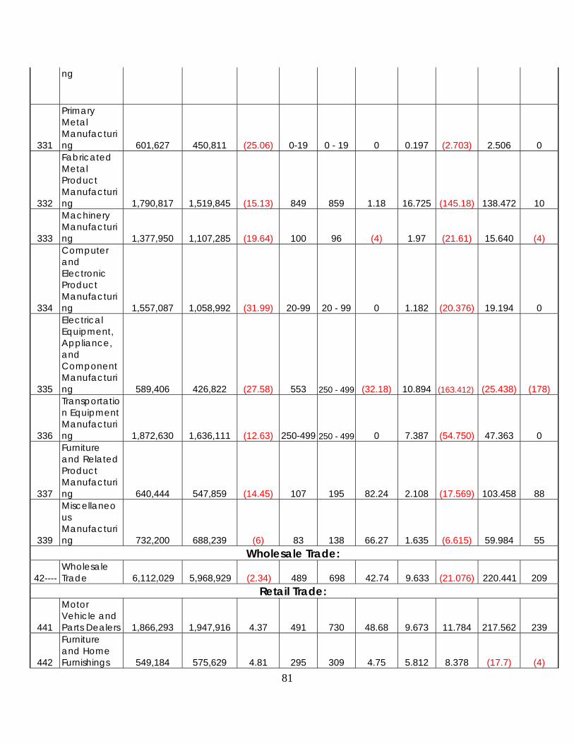
81

ng

331

Primary Metal Manufacturing 601,627 450,811 (25.06) 0-19 0 - 19 0 0.197 (2.703) 2.506 0

332

Fabricated Metal Product Manufacturing 1,790,817 1,519,845 (15.13) 849 859 1.18 16.725 (145.18) 138.472 10

333

Machinery Manufacturing 1,377,950 1,107,285 (19.64) 100 96 (4) 1.97 (21.61) 15.640 (4)

334

Computer and Electronic Product Manufacturing 1,557,087 1,058,992 (31.99) 20-99 20 - 99 0 1.182 (20.376) 19.194 0

335

Electrical Equipment, Appliance, and Component Manufacturing 589,406 426,822 (27.58) 553 250 - 499 (32.18) 10.894 (163.412) (25.438) (178)

336

Transportation Equipment Manufacturing 1,872,630 1,636,111 (12.63) 250-499 250 - 499 0 7.387 (54.750) 47.363 0

337

Furniture and Related Product Manufacturing 640,444 547,859 (14.45) 107 195 82.24 2.108 (17.569) 103.458 88

339

Miscellaneous Manufacturing 732,200 688,239 (6) 83 138 66.27 1.635 (6.615) 59.984 55

Wholesale Trade:

42---- Wholesale Trade 6,112,029 5,968,929 (2.34) 489 698 42.74 9.633 (21.076) 220.441 209

Retail Trade:

441

Motor Vehicle and Parts Dealers 1,866,293 1,947,916 4.37 491 730 48.68 9.673 11.784 217.562 239

442

Furniture and Home Furnishings 549,184 575,629 4.81 295 309 4.75 5.812 8.378 (17.7) (4)

82

Stores

443

Electronics and Appliance Stores 407,321 469,248 15.20 236 165 (30.08) 4.649 31.223 (106.861) (71)

444

Building Material and Garden Equipment and Supplies Dealers 1,235,387 1,262,662 2.21 356 448 25.84 7.19 0.854 84.123 92

445

Food and Beverage Stores 3,004,410 2,937,918 (2.21) 687 914 33.04 13.534 (28.717) 242.168 227

446

Health and Personal Care Stores 913,896 1,037,354 13.51 161 247 53.42 3.172 18.579 64.255 86

447 Gasoline Stations 937,083 908,818 (3.02) 366 364 (0.01) 7.21 (18.263) 11.017 (0)

448

Clothing and Clothing Accessories Stores 1,368,665 1,555,928 13.68 1,210 2,357 94.79 23.837 14.169 98.143 136

451

Sporting Goods, Hobby, Book, and Music Stores 616,237 631,095 2.41 109 280 156.88 2.147 0.480 168.372 171

452

General Merchandise Stores 2,526,107 2,670,710 5.72 560 651 16.25 11.032 21 58.968 91

453

Miscellaneous Store Retailers 849,661 819,903 (3.50) 401 349 (12.97) 7.899 (21.935) (37.975) (52)

454 Nonstore Retailers 566,531 521,491 (7.95) 70 113 61.43 1.379 (6.944) 48.566 43

Transportation & Warehousing:

481

Air Transportation 615,605 486,355 (20.99) 20-99 20 - 99 0 1.182 (13.776) 12.594 0

484

Truck Transportation 1,415,794 1,478,299 4.41 115 168 46.09 2.266 2.806 47.932 53

486

Pipeline Transportation 52,960 38,053 (28.15) 1 0 - 19 900 0.02 (0.301) 9.282 9

488

Support Activities for Transportatio 472,372 543,666 15.09 51 52 1.96 1.005 6.691 (6.696) 1

83

n

492 Couriers and Messengers 619,313 547,255 (11.64) 0-19 20 - 99 500 0.197 (1.361) 51.164 50

493

Warehousing and Storage 135,898 578,040 325.35 0-19 250 - 499 3,650 0.197 32.338 332.465 365

Information: 51---- Information 3,545,731 3,402,599 (4.04) 469 629 34.12 9.239 (28.187) 178.970 160

Finance and Insurance:

522

Credit Intermediation and Related Activities 2,753,190 3,201,715 16.29 349 417 19.48 6.875 49.978 13.302 70

523

Securities, Commodity Contracts, and Other Financial Investments and Related Activities 866,222 860,384 (0.01) 20-99 48 (20) 1.182 (1.188) (11.994) (12)

524

Insurance Carriers and Related Activities 2,290,162 2,323,045 1.44 94 147 56.38 1.852 (0.498) 51.644 53

Real estate & rental & leasing: 531 Real Estate 1,279,547 1,480,040 15.67 100-249 308 76 3.448 23.975 105.578 133

532

Rental and Leasing Services 636,037 634,901 0 20-99 100 - 249 191.67 1.182 (1.182) 115.002 115

533

Lessors of Nonfinancial Intangible Assets (except Copyrighted Works) 26,462 29,136 10.11 0-19 0 - 19 0 0.197 0.814 (1.011) 0

Professional, scientific, & technical services:

541

Professional, Scientific, and Technical Services 6,816,216 7,689,366 12.81 612 1,469 140.03 12.056 66.341 778.586 78

Management of companies and enterprises:

551

Management of Companies and Enterprises 2,873,521 2,856,418 (0.01) 544 344 (36.76) 10.717 (10.771) (199.920) (200)

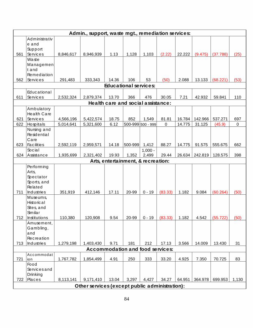
84

Admin., support, waste mgt., remediation services:

561

Administrative and Support Services 8,846,617 8,946,939 1.13 1,128 1,103 (2.22) 22.222 (9.475) (37.788) (25)

562

Waste Management and Remediation Services 291,483 333,343 14.36 106 53 (50) 2.088 13.133 (68.221) (53)

Educational services:

611 Educational Services 2,532,324 2,879,374 13.70 366 476 30.05 7.21 42.932 59.841 110

Health care and social assistance:

621

Ambulatory Health Care Services 4,566,196 5,422,574 18.75 852 1,549 81.81 16.784 142.966 537.271 697

622 Hospitals 5,014,641 5,321,600 6.12 500-999 500 - 999 0 14.775 31.125 (45.9) 0

623

Nursing and Residential Care Facilities 2,592,119 2,959,571 14.18 500-999 1,412 88.27 14.775 91.575 555.675 662

624 Social Assistance 1,935,699 2,321,402 19.93 1,352

1,000 - 2,499 29.44 26.634 242.819 128.575 398

Arts, entertainment, & recreation:

711

Performing Arts, Spectator Sports, and Related Industries 351,919 412,146 17.11 20-99 0 - 19 (83.33) 1.182 9.084 (60.264) (50)

712

Museums, Historical Sites, and Similar Institutions 110,380 120,908 9.54 20-99 0 - 19 (83.33) 1.182 4.542 (55.722) (50)

713

Amusement, Gambling, and Recreation Industries 1,279,198 1,403,430 9.71 181 212 17.13 3.566 14.009 13.430 31

Accommodation and food services:

721 Accommodation 1,767,782 1,854,499 4.91 250 333 33.20 4.925 7.350 70.725 83

722

Food Services and Drinking Places 8,113,141 9,171,410 13.04 3,297 4,427 34.27 64.951 364.978 699.953 1,130

Other services (except public administration):

85

811

Repair and Maintenance 1,334,206 1,294,783 (2.95) 289 486 68.17 5.693 (14.219) 205.537 197

812

Personal and Laundry Services 1,293,215 1,337,443 3.42 217 360 65.90 4.275 3.147 135.582 143

813

Religious, Grantmaking, Civic, Professional, and Similar Organizations 2,665,978 2,758,728 3.48 513 751 46.39 10.106 7.746 220.128 238

Unclassified establishments:

99----

Unclassified establishments 143,600 31,153 (78.31) 53 4 (92.45) 1.004 (42.548) (7.494) (49)

TOTAL U.S. Employment 114,064,976 116,317,003 1.97 24,040 31,466 30.89 475.87 460.97 6,109.32 7,057.60

***Obtained by dividing ending year employment by beginning year employment , then subtracting one and moving decimal two places to the right

***For non-specific employment figures, calculations were made using the mean***