regional evaluation of satellite‐based methods for

ORIGINAL RESEARCH

Regional evaluation of satellite-based methods foridentifying end of vegetation growing seasonRuoque Shen1, Haibo Lu1 , Wenping Yuan1, Xiuzhi Chen1 & Bin He2

1School of Atmospheric Sciences, Southern Marine Science and Engineering Guangdong Laboratory (Zhuhai), Sun Yat-sen University, Zhuhai

Guangdong, 519082, China2College of Global Change and Earth System Science, Beijing Normal University, Beijing 100038, China

Keywords

Autumn phenology, end of growing season

dates, remote sensing, satellite-based

methods, vegetation index

Correspondence

Haibo Lu, School of Atmospheric Sciences,

Southern Marine Science and Engineering

Guangdong Laboratory (Zhuhai), Sun Yat-sen

University, Zhuhai, Guangdong 519082,

China. Tel: +86 0756-3668166; Fax: +860756-3668166; E-mail:

[email protected]

Handling Editor: Mat Disney

Associate Editor: Doreen Boyd

Received: 20 October 2020; Revised: 16 May

2021; Accepted: 25 May 2021

doi: 10.1002/rse2.223

Abstract

Autumn phenology plays an important role in regulating ecosystem carbon and

water cycling, but it has received less attention than spring phenology. Satellite-

based methods have been widely applied in monitoring autumn phenology at

large spatial scales. However, few studies have evaluated and compared the per-

formance of different satellite-based methods in autumn phenology identifica-

tion. Here, we compared the spatiotemporal variations of end of vegetation

growing season dates (EOS) as determined from eight prevailing satellite-based

methods against long-term field observations at 31 sites in China. We found

that field-based observations in forest and grassland sites, respectively, had rates

of EOS delay of 2.11 and 3.85 days per 1°C increase in mean annual tempera-

ture (MAT) during 2001–2014. However, nearly all the eight satellite-based

methods underestimated these delay rates compared with the ground observa-

tions over all sites. We also found that the eight methods weakly agreed with

the field-observed interannual variations of EOS. At the regional scale, the iden-

tified average EOS differed up to 38 and 40 days among the investigated

satellite-based methods in forest and grassland ecosystems respectively. The

delayed rate of identified EOS with the increase of MAT ranged from 0.77 to

3.51 days °C−1 for forests and from 0.41 to 2.95 days °C−1 for grasslands. The

identified EOS by most of the eight methods had delayed temporal trends in

forests during 2001–2014 while we found advanced trends in grassland ecosys-

tems. The large discrepancy in EOS identification among the prevailing

satellite-based methods highlight the need for more accurate satellite-based

methods in data gap-filling and phenometrics detection, and more extensive,

multi-species based field observations that can be used to constrain and validate

the satellite-based methods.

Introduction

A critical process during vegetation growth, autumn

phenology (i.e., leaf coloration, senescence and dor-

mancy) directly regulates the length of growing season

and has important implications for the carbon and

nutrient cycling of terrestrial ecosystem (Keenan et al.,

2014; Penuelas & Filella, 2009). The dates of end of veg-

etation growing season (EOS) have been widely shown

to be susceptible to climate change (e.g., warming and

drought) (Gallinat et al., 2015; Xie et al., 2015). In par-

ticular, numerous studies have reported that the rising

autumn temperature induced by climate warming has

delayed the EOS (Garonna et al., 2014; Ge et al., 2015;

Piao et al., 2006). Moreover, EOS has showed a larger

sensitivity to temperature than spring leaf-out phenol-

ogy, which implied that delayed EOS can contribute

more to the extension of the growing season than

advanced spring leaf-out under global warming (Fu

et al., 2018; Garonna et al., 2014). Thus, the accurate

identification of the spatiotemporal changes of EOS over

regional scale is essential for revealing the impacts of

phenological changes on regional carbon budgets and

ecosystem function.

ª 2021 The Authors. Remote Sensing in Ecology and Conservation published by John Wiley & Sons Ltd on behalf of Zoological Society of London

This is an open access article under the terms of the Creative Commons Attribution-NonCommercial-NoDerivs License, which permits use and

distribution in any medium, provided the original work is properly cited, the use is non-commercial and no modifications or adaptations are made.

1

https://orcid.org/0000-0002-2461-4870

https://orcid.org/0000-0002-2461-4870

https://orcid.org/0000-0002-2461-4870

mailto:

http://creativecommons.org/licenses/by-nc-nd/4.0/

Current field studies revealed the impacts of climate

change on autumn plant phenology over the past decades.

Ge et al. (2015) conducted a meta-analysis of Chinese

phenological responses to climate change across 145 sites

and found that autumn phenology was delayed by 1.93–4.84 days decade−1 during 1960–2011 in China. Menzel

et al. (2006) reported that leaf coloring and senescence

delayed by 1.0 day °C−1 during 1971–2000 in Europe. In

North America continent, Jeong and Medvigy (2014)

found a delay trend of 0.36 day year−1 in all-species aver-

age leaf coloring date.

The availability of global remote sensing vegetation

index (VI) datasets in recent decades has yielded the abil-

ity to monitor regional and global land surface phenology

(LSP). The satellite-based methods, which are based on

the analysis of the seasonal dynamics of VI time series,

has offered a continuous and robust way to monitor plant

phenology at large spatial scales (Reed et al., 2009; Zhang

et al., 2006). Generally, three primary procedures were

conducted in the satellite-based methods to estimate the

EOS: first, cleaning and flagging the noisy data in original

VI products; second, smoothing and reconstructing VI

time series curves using curve fitting methods (e.g., logis-

tic, Gaussian-midpoint, harmonic analysis of time series

(HANTS) and polyfit maximum); third, determining the

EOS dates by identifying the inflection of the transition

point from the reconstructed VI curve or predefined

threshold of the VI (Berra & Gaulton, 2021; Zeng et al.,

2020). For example, Zhang et al. (2003) developed a

piecewise logistic function to fit time series normalized

difference vegetation index (NDVI) data and identified

the key phenological transition dates through the changes

in curvature. Garonna et al. (2014) employed the HANTS

approach to reconstruct NDVI time series and derived

the EOS dates across Europe using a local NDVI thresh-

old. Moreover, Alberton et al. (2019) deployed General-

ized Additive Mixed Models (GAMMs) to estimate the

timing and length of growing season based on phenocam-

eras networks observations. Recently, Belda et al. (2020)

applied advanced machine learning algorithms for VI

curves reconstruction and estimated phenological indica-

tors for specific crop types.

However, large discrepancies among the prevailing

satellite-based methods have been observed for identifying

phenological timing (Berra & Gaulton, 2021; Zeng et al.,

2020). A comprehensive intercomparison is still lacking,

particularly for evaluating the performance of the meth-

ods in determining EOS against long-term observations

over multiple ecosystems and geographic regions. de

Beurs and Henebry (2010) evaluated 12 state-of-the-art

remote sensing methods for modeling LSP, and they

found differences as high as 100 days in the estimated

EOS dates between individual methods. Recently, Xin

et al. (2020) compared six commonly used satellite-based

methods and two machine learning methods to retrieve

EOS, the differences among different methods ranged

from 11.60 to 44.34 days. Thus, a comprehensive evalua-

tion and interpretation of the spatiotemporal variation of

EOS derived from the satellite-based methods should be

conducted to better understand their performance and

how they differ from field-based observations.

Here, we evaluated and compared the performance of

eight prevailing satellite-based methods for determining

EOS against long-term field observations at 31 sites in

China. Our primary objectives were to (1) evaluate the

performance of the eight satellite-based methods on

reproducing the spatiotemporal variations of EOS against

field-based observations, and (2) compare the differences

among the satellite-based methods in identifying the spa-

tiotemporal pattern of regional EOS during 2001 to 2014

in China.

Materials and Methods

Study area

In this study, the temperate and deciduous broadleaf for-

ests dominated northern subtropical areas in China were

selected for autumn phenology investigation. These areas

included vegetation types of deciduous broadleaf forest

(DBF), deciduous needleleaf forest (DNF), mixed forest

(MF), and grassland. The evergreen broadleaf forest

(EBF) and evergreen needleleaf forest (ENF) regions were

excluded due to lack of seasonal dynamics. The cropland

areas of which phenology are largely affected by human

activity were also not included in this study.

Satellite-based EOS identification methods

We evaluated the performance of eight prevailing

satellite-based methods for determining EOS dates. Each

satellite-based EOS detection method consists of a curve

fitting method for reconstructing NDVI time series and a

phenological metrics extraction method to derivate the

EOS dates. In total, there are eight NDVI curve fitting

methods and four phenological metrics extraction meth-

ods being applied in the eight investigated satellite-based

methods. All the eight methods were described in Table 1.

To explore the effects of different NDVI curve fitting

and phenological metrics detection methods on the per-

formance of the eight satellite-based methods, the eight

curve fitting methods and four phenological metrics

detection methods were recombined. We generated 30

method combinations, including 22 new methods in addi-

tion to the eight original methods (Table 2). The

2 ª 2021 The Authors. Remote Sensing in Ecology and Conservation published by John Wiley & Sons Ltd on behalf of Zoological Society of London

Regional Evaluation of Satellite-based EOS Methods R. Shen et al.

performances of all the 30 methods on estimating the

spatiotemporal variations of EOS were evaluated and

intercompared against the ground observations.

Data

Phenological observations in China

In this study, the ground observations of leaf senescence

date were defined as observed EOS. The long-term, field-

observed records of leaf senescence date in China used in

this study were sourced from two datasets: the Chinese

Phenological Observation Network (CPON) for woody

plants and the Chinese Ecosystem Research Network

(CERN) Phenology Dataset for herbaceous plants (Song

et al., 2017). At both CPON and CERN observation sites,

the same standardized criteria for field measurements

were followed (Wan & Liu, 1979). Most of these observa-

tion sites locate at long-term ecological observation sta-

tions in China and the rest locate at botany gardens and

natural parks. To represent the phenology of multiple

species, only when the observations covered at least 20

tree or 5 herbaceous species during 2001–2014, could the

observation sites be included in this study. In total, we

Table 1. Description of the eight satellite-based methods for EOS identification.

Methods NDVI curve fitting methods

Phenological metrics detection

methods References

Simple logistic

method

NDVI tð Þ¼ a1þ a21þexp a3þa4tð Þ Change rate of curvature K¼ dα

ds

� �Zhang et al. (2003)

Double logistic

method

NDVI tð Þ¼ a1þ a2�a7tð Þ 1

1þexp a�ta4

� �� 1

1þexp a�ta6

� �24

35 Change rate of curvature Elmore et al. (2012)

Generalized

double

logistic

method

NDVI tð Þ¼ a1tþb1ð Þþ a2t2þb2tþc

� �1

½1þq1e�h1 t�n1ð Þ �v1

1

½1þq2e�h2 t�n2ð Þ �v2

� �Change rate of curvature Klosterman et al.

(2014)

Gaussian-

midpoint

method

NDVI tð Þ¼ aþb�e�t�cdð Þ2 0.5 of the NDVI amplitude

NDVIðtÞratio ¼ NDVI tð Þ�Min NDVIð ÞMax NDVIð Þ�Min NDVIð Þ

� � White et al. (2009)

Spline-

midpoint

method

NDVI tð Þ¼ att3þjbtt2þcttþdt 0.5 of the NDVI amplitude White et al. (2009)

HANTS-

maximum

method

NDVI tð Þ¼ a0þ∑n

i¼1

aicos ωi t�φið Þ Local NDVI ratio

NDVIratio tð Þ¼ NDVI tþ1ð Þ�NDVI tð ÞNDVI tð Þ

� � Jakubauskas et al.

(2001) and Garonna

et al. (2014)

Polyfit-

maximum

method

NDVI tð Þ¼ a0þa1tþa2t2þa3t

3þa4t4þa5t

5þa6t6 Local NDVI ratio Piao et al. (2006)

Timesat SG

method

Savitzky-Golay (SG) filtering method 0.2 of the NDVI amplitude Savitzky and Golay

(1964)

t is the day of year; NDVI(t) indicates the NDVI value on tth day; a0 to a6, a, b, b1, b2, c, d, h1, h2, n1, n2, q1, q2, v1 and v2 are curve fitting param-

eters; K indicates the curvature.

Table 2. Recombination of the eight NDVI curve fitting methods and

four phenological metrics detection methods.

NDVI curve

fitting

methods

Phenological metrics detection methods

Change

rate of

curvature

Local

NDVI

ratio

0.2 of the

NDVI

amplitude

0.5 of the

NDVI

amplitude

Simple logistic *Sim Sim2 Sim3 Sim4

Double logistic *Dou Dou2 Dou3 Dou4

Generalized

double

logistic

*Gen Gen2 Gen3 Gen4

Gaussian Gau1 Gau2 Gau3 *GauSpline Spl1 Spl2 Spl3 *SplHANTS HAN1 *HAN HAN3 HAN4

Polyfit Pol1 *Pol Pol3 Pol4

Timesat SG / / *SG SG4

*The asterisks indicate the eight original methods and the other indi-

cate the 22 new combinations. For example, *Sim indicates the origi-

nal method of the simple logistical curve fitting method combining

with the change rate of curvature method; Sim2, Sim3, and Sim4

indicate three new generated methods, that is, the simple logistical

curve fitting method combining with the local NDVI ratio, the 0.2 of

the NDVI amplitude and the 0.5 of the NDVI amplitude method

respectively.

ª 2021 The Authors. Remote Sensing in Ecology and Conservation published by John Wiley & Sons Ltd on behalf of Zoological Society of London 3

R. Shen et al. Regional Evaluation of Satellite-based EOS Methods

included observations of 1035 plant species (737 tree and

298 herbaceous species) at 31 sites ranging from 25 to

53°N (Fig. 1, Table S1). To examine the temporal trend

of autumn plant phenology, we further selected 25 sites

that had observations longer than 10 years during 2001–2014, eventually there were 6226 observations from 266

tree and 58 herbaceous species remained for temporal

variation analysis (Table S1). In addition, the leaf senes-

cence date in this study was defined as the end of leaf fall,

which represents the date on which 95% of the leaves on

the monitored plants had fallen (Wan & Liu, 1979).

Satellite and meteorology data

The land surface EOS dates during 2001–2014 were

derived from the NDVI time series data (MOD13C1)

from the Moderate Resolution Imaging Spectroradiometer

(MODIS) Version 6 datasets (https://e4ftl01.cr.usgs.gov//

MODV6_Cmp_C/MOLT/MOD13C1.006/). The temporal

and spatial resolution of the NDVI data we used were

16 days and 5 km. The daily surface air temperature data-

set at a spatial resolution of 0.1° during 2001–2014 was

from the China Meteorological Forcing Dataset (CMFD)

product (He et al., 2020), which was used for calculating

mean annual temperature (MAT). The vegetation types of

study area were derived from the MODIS land cover pro-

duct (MOD12Q1, V004) at a spatial resolution of 1 km

(Ran et al., 2010). The air temperature and land cover

datasets were resampled to the spatial resolution of 0.05°to match the NDVI dataset.

Data analysis

In order to compare satellite-based EOS with ground

observed leaf senescence dates (i.e., observed EOS) at each

observation site, we selected 20 pixels which had the same

vegetation type and were nearest to each observation site

to retrieve EOS. These pixels were all around the observa-

tions site within 100 km range. NDVI time series of each

pixel was extracted and EOS was determined using the

eight satellite-based methods. Then, the averaged EOS

from the 20 pixels was used to compare against the

ground observation.

To examine the spatial variations of EOS, linear regres-

sion analysis was conducted between MAT and the

satellite-based and ground observed mean annual EOS

over all the 31 sites. At the 25 observation sites which

had long-term (>10 years) ground observations, we

Figure 1. Descriptions of the study area and the location of ground phenology observation sites.



https://e4ftl01.cr.usgs.gov//MODV6_Cmp_C/MOLT/MOD13C1.006/

https://e4ftl01.cr.usgs.gov//MODV6_Cmp_C/MOLT/MOD13C1.006/

detected the temporal trends of satellite-based and ground

observed EOS during 2001–2014.

Results

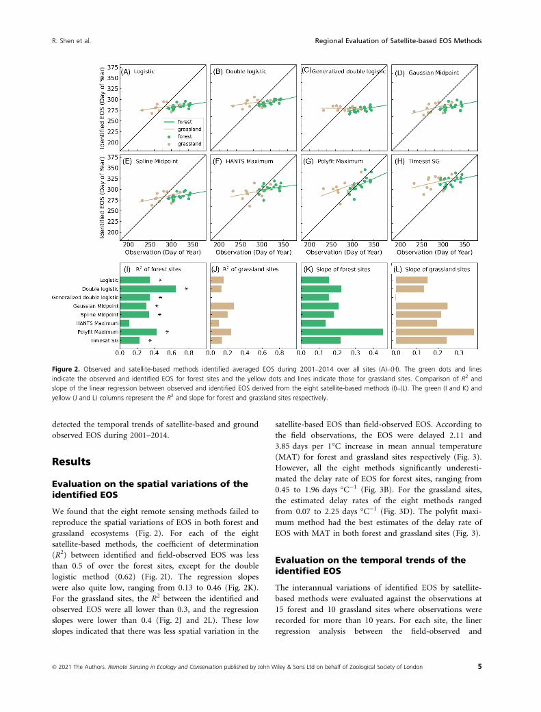
Evaluation on the spatial variations of theidentified EOS

We found that the eight remote sensing methods failed to

reproduce the spatial variations of EOS in both forest and

grassland ecosystems (Fig. 2). For each of the eight

satellite-based methods, the coefficient of determination

(R2) between identified and field-observed EOS was less

than 0.5 of over the forest sites, except for the double

logistic method (0.62) (Fig. 2I). The regression slopes

were also quite low, ranging from 0.13 to 0.46 (Fig. 2K).

For the grassland sites, the R2 between the identified and

observed EOS were all lower than 0.3, and the regression

slopes were lower than 0.4 (Fig. 2J and 2L). These low

slopes indicated that there was less spatial variation in the

satellite-based EOS than field-observed EOS. According to

the field observations, the EOS were delayed 2.11 and

3.85 days per 1°C increase in mean annual temperature

(MAT) for forest and grassland sites respectively (Fig. 3).

However, all the eight methods significantly underesti-

mated the delay rate of EOS for forest sites, ranging from

0.45 to 1.96 days °C−1 (Fig. 3B). For the grassland sites,

the estimated delay rates of the eight methods ranged

from 0.07 to 2.25 days °C−1 (Fig. 3D). The polyfit maxi-

mum method had the best estimates of the delay rate of

EOS with MAT in both forest and grassland sites (Fig. 3).

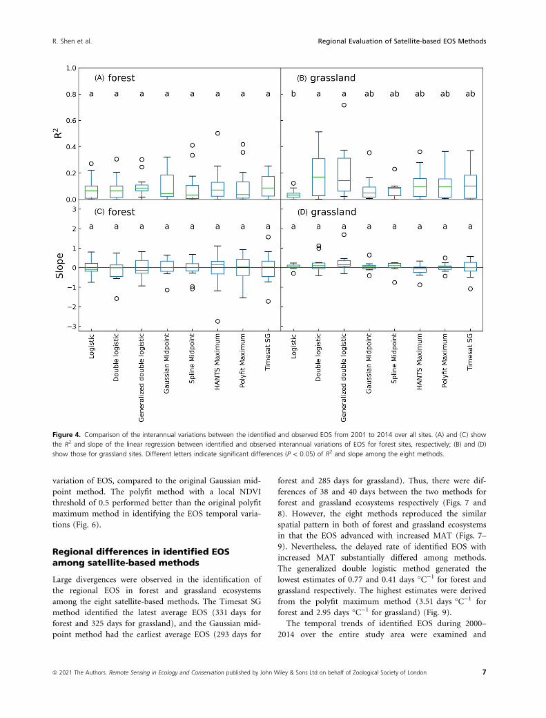
Evaluation on the temporal trends of theidentified EOS

The interannual variations of identified EOS by satellite-

based methods were evaluated against the observations at

15 forest and 10 grassland sites where observations were

recorded for more than 10 years. For each site, the liner

regression analysis between the field-observed and

Figure 2. Observed and satellite-based methods identified averaged EOS during 2001–2014 over all sites (A)–(H). The green dots and lines

indicate the observed and identified EOS for forest sites and the yellow dots and lines indicate those for grassland sites. Comparison of R2 and

slope of the linear regression between observed and identified EOS derived from the eight satellite-based methods (I)–(L). The green (I and K) and

yellow (J and L) columns represent the R2 and slope for forest and grassland sites respectively.



identified EOS was employed to examine the performance

of the remote sensing methods. Generally, the eight meth-

ods showed poor performance in capturing the interan-

nual variations of EOS across the forest and grassland

sites (Fig. 4). The mean R2 values across all sites were

quite low, ranging from 0.05 to 0.11 for forest and 0.06

to 0.18 for grassland sites among the eight satellite-based

methods respectively (Fig. 4A and B). The corresponding

slopes of the regression lines also deviated broadly from 1

at both forest and grassland sites (Fig. 4C and D).

The temporal trends of identified EOS by satellite-

based methods at each site were also compared with the

observations. Large variations in the trend of field-

observed EOS existed among the observation sites. The

eight methods performed poorly at estimating the tempo-

ral trends in both forest and grassland sites (Fig. 5).

Compared to the field-observed trends, the generalized

double logistic and the timesat SG methods significantly

underestimated the trends at 60% forest sites whereas the

Logistic, the HANTS maximum and the polyfit maximum

methods overestimated the trends at more than 40% for-

est sites (Fig. 5B). For grasslands sites, each of the eight

methods significantly overestimated the trends. The

HANTS maximum and the timesat SG methods showed

significantly higher estimates in more than 40% grass-

lands sites (Fig. 5D).

Comparisons of the method structure

We found that most of the 22 newly recombined methods

did not perform better than the eight original methods in

reproducing the spatial and temporal variations of the

EOS. That implied that the eight original methods were

the best among the potential combinations (Fig. 6). How-

ever, the Gaussian method with the NDVI ratio approach

improved the performance in capturing the temporal

Figure 3. Spatial variations of the observed and satellite-based methods identified EOS with the mean annual temperature (MAT) increasing for

forest (A) and grassland (C) sites. (B) and (D) showed the slope of regression lines which indicates the delay rate of EOS with the rising MAT. The

letters indicate the statistically significant (P < 0.05) difference among observations and estimates.



variation of EOS, compared to the original Gaussian mid-

point method. The polyfit method with a local NDVI

threshold of 0.5 performed better than the original polyfit

maximum method in identifying the EOS temporal varia-

tions (Fig. 6).

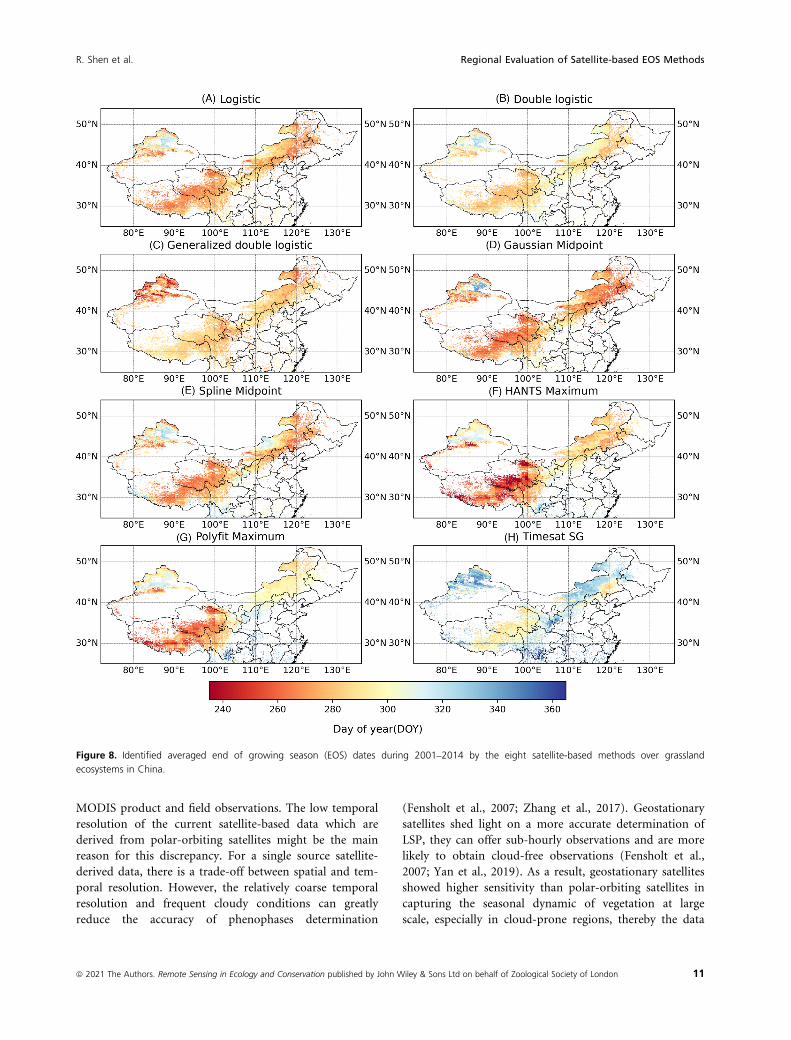
Regional differences in identified EOSamong satellite-based methods

Large divergences were observed in the identification of

the regional EOS in forest and grassland ecosystems

among the eight satellite-based methods. The Timesat SG

method identified the latest average EOS (331 days for

forest and 325 days for grassland), and the Gaussian mid-

point method had the earliest average EOS (293 days for

forest and 285 days for grassland). Thus, there were dif-

ferences of 38 and 40 days between the two methods for

forest and grassland ecosystems respectively (Figs. 7 and

8). However, the eight methods reproduced the similar

spatial pattern in both of forest and grassland ecosystems

in that the EOS advanced with increased MAT (Figs. 7–9). Nevertheless, the delayed rate of identified EOS with

increased MAT substantially differed among methods.

The generalized double logistic method generated the

lowest estimates of 0.77 and 0.41 days °C−1 for forest and

grassland respectively. The highest estimates were derived

from the polyfit maximum method (3.51 days °C−1 for

forest and 2.95 days °C−1 for grassland) (Fig. 9).

The temporal trends of identified EOS during 2000–2014 over the entire study area were examined and

Figure 4. Comparison of the interannual variations between the identified and observed EOS from 2001 to 2014 over all sites. (A) and (C) show

the R2 and slope of the linear regression between identified and observed interannual variations of EOS for forest sites, respectively; (B) and (D)

show those for grassland sites. Different letters indicate significant differences (P < 0.05) of R2 and slope among the eight methods.



substantial divergences of identified trends were found

among the eight methods. Most of the methods showed

the delayed temporal trends of EOS for forests with the

averaged rates from 0.32 to 0.52 day year−1 over the study

area, except for the generalized double logistic and the

timesat SG method which identified averaged advanced

trends of −0.26 and −0.41 day year−1 respectively (Fig. 10

A). On the contrary, most of the eight methods generated

advanced temporal trends for grassland, ranging from

0.05 to 0.44 day year−1. Only the HANTS maximum

(0.17 day year−1) and the polyfit maximum method

(0.02 day year−1) showed delayed temporal trends

(Fig. 10B).

Discussion

As one of the most reliable and robust approach to moni-

tor LSP at large spatial scales, satellite-based methods are

widely employed to monitor phenology dynamics and its

responses to climate changes at global and regional scales

(Reed et al., 2009; Zeng et al., 2020; Zhang et al., 2003).

However, our study showed that the prevailing eight

satellite-based methods performed poorly at identifying

the temporal and spatial variations of EOS against the

ground observations at the 31 sites (Figs. 2–5). Thus, one

should be cautious that when interpreting the temporal

and spatial variations of satellite-based EOS using the

eight methods we investigated. The discrepancy between

the identified EOS by the remote sensing methods and

the ground observations was also reported in the previous

studies. Zhao et al. (2020) reported that the autumn phe-

nology dates derived from satellite data was consistently

earlier than that from direct observations in a northern

mixed forest. Such a discrepancy may be attributed to the

satellite data having had a relatively coarse spatial resolu-

tion and thus integrated a broader vegetation signal

across a heterogeneous landscape than the field individual

species observation. The incompatibility of spatial scales

and mixed pixel effects might induce uncertainty when

evaluating and constraining the performance of satellite-

based EOS against ground in situ observations (Chen

et al., 2018; Donnelly et al., 2018; Liang et al., 2011; Zeng

et al., 2020). Hence, it is necessary to extend the field

observations of autumn phenology covering multiple

plant species and various ecosystem types to reduce the

uncertainty in benchmarking and improving the satellite-

based LSP algorithms.

Furthermore, large divergences in detecting the spa-

tiotemporal variations of EOS were also observed among

the different methods (Figs. 7–9), which was supported

Figure 5. Temporal trends of identified and observed EOS for forest (A, B) and grassland (C, D) sites. The observations are presented as hollow

dots with an error bar which indicates the standard deviation of the trend of each plant species, and the colorful dots/stars indicate the estimated

trends by the satellite-based methods (A, C). (B) and (D) show the percentage of sites in which the identified trends lower or higher than the

observations (significance level at P < 0.05).



by previous studies. de Beurs and Henebry (2010) con-

ducted a comparison of 10 common remote sensing

methods for detecting phenology, and the differences in

identified growing season length were as much as 64 to

190 days among methods. We found that the polyfit max-

imum method performed best at estimating EOS when

compared to field observations. This better match could

be because the polyfit-maximum method is a high-order

Fourier transforms, which reconstructs the VI curve

through the entire growing season with the highest tem-

poral resolution (i.e., daily) (Piao et al., 2006). The other

seven methods reconstruct the VI curve at the original

temporal resolution (i.e., 16-day). The wide applications

of machine learning approaches open a new path to the

development of satellite-based phenology models.

Recently, Belda et al. (2020) blended machine learning

algorithms (e.g., Gaussian Process Regression, GPR) using

leaf area index (LAI) curve reconstruction in satellite-

based phenology methods, the new methods successfully

reconstructed LAI curves and retrieved reliable

phenological indicators. Leaf falling phase is a transient

process, the curve fitting method with higher resolution

can better capture the phenological information (Her-

mance, 2007). Moreover, the VI trajectory during the leaf

coloring and senescence phase could appear as a two-

stage decline, that is, before a rapid drop-off, there may

exist a gradual decrease in the VI, which could last several

weeks to months (Elmore et al., 2012; Guyon et al., 2011;

Zeng et al., 2020). In this study, we also observed the

gradual decrease of NDVI before EOS dates, such a two-

stage decline can complicate the detection of the autumn

phenological transition dates. In addition, our results

showed that nearly all the investigated satellite-based

methods identified advanced temporal trend of regional

EOS for grassland ecosystem while generated delayed tem-

poral trend for forest ecosystems (Fig. 10). The advanced

EOS trend of grasslands was also reported by Ren et al.

(2017) who found that 65% of Inner Mongolia plateau in

China showed earlier EOS trend during 2000–2011. Theadvanced EOS trends for grasslands can attribute to a

Figure 6. Comparison of the various combinations of the eight NDVI curve fitting methods and four transition point detection methods in

reproducing the spatial (A, B) and temporal (C, D) trends of identified EOS against observations. The R2 and slope derive from the linear

regression of identified and observed EOS. The white bars indicate the original combinations of the eight methods.



decline in precipitation from mid-1990s onward and soil

water deficit induced by climate warming (Bao et al.,

2021; Guo et al., 2021; Wang et al., 2019).

The remote sensing methods have been widely used to

generate LSP products, such as the MODIS Global Vege-

tation Phenology product (MCD12Q2) (Friedl et al.,

2019) and the Visible Infrared Imaging Radiometer Suite

(VIIRS) LSP product (Zhang et al., 2018). Our results

implied that the prevailing LSP products derived from

satellite data may have large uncertainty in EOS identifi-

cation, which can further impede our understanding on

the responses of autumn phenology to climate change at

regional and global scale. Hmimina et al. (2013) evaluated

the MODIS phenology product against field observations

and found that the biases were more than two weeks dur-

ing the autumn phenological transitions between the

Figure 7. Identified averaged end of growing season (EOS) dates during 2001–2014 by the eight satellite-based methods over forest ecosystems

in China.



MODIS product and field observations. The low temporal

resolution of the current satellite-based data which are

derived from polar-orbiting satellites might be the main

reason for this discrepancy. For a single source satellite-

derived data, there is a trade-off between spatial and tem-

poral resolution. However, the relatively coarse temporal

resolution and frequent cloudy conditions can greatly

reduce the accuracy of phenophases determination

(Fensholt et al., 2007; Zhang et al., 2017). Geostationary

satellites shed light on a more accurate determination of

LSP, they can offer sub-hourly observations and are more

likely to obtain cloud-free observations (Fensholt et al.,

2007; Yan et al., 2019). As a result, geostationary satellites

showed higher sensitivity than polar-orbiting satellites in

capturing the seasonal dynamic of vegetation at large

scale, especially in cloud-prone regions, thereby the data

Figure 8. Identified averaged end of growing season (EOS) dates during 2001–2014 by the eight satellite-based methods over grassland

ecosystems in China.



Figure 9. Spatial variations of identified regional EOS for forest (A) and grassland (B) ecosystems with the rising mean annual temperature (MAT).

(C) Shows the delayed rate of EOS with the rising MAT.

Figure 10. Long-term trends of identified EOS derived from the eight satellite-based methods for forest (A) and grassland (B) ecosystems.



from geostationary satellites can be a better choice for

determining LSP (Fensholt et al., 2007).

Conclusions

Satellite-based methods were widely applied to monitor

phenology at regional and global scale. In this study, we

evaluated the performance of eight prevailing satellite-

based methods for EOS identification against long-term

field observations at 31 sites in China. Our results indi-

cated that nearly all the eight investigated methods under-

estimated the variations of EOS with increasing MAT for

both forest and grassland ecosystems when compared to

the field observations. We also found that the eight meth-

ods weakly agreed with the field-observed interannual

variations of EOS, which implied large uncertainty of

satellite-based EOS in response to climate change. More-

over, substantial discrepancies of estimated regional EOS

existed among the eight satellite-based methods. The

identified EOS by most of the eight methods had delayed

temporal trends in forests during 2001-2014 while we

found advanced trends in grassland ecosystems. Our

study highlighted that the prevailing satellite-based meth-

ods had large uncertainty in identifying autumn phenol-

ogy, and cautions should be used when drawing

conclusion about the changes of autumn phenology based

on the eight methods. This study also suggested a need

for more accurate satellite-based methods to determine

EOS, and more extensive, species-based field observations

that can be used to constrain and validate the satellite-

based methods.

Acknowledgments

This study was funded by the National Key Basic Research

Program of China (2018YFA0606104, 2016YFA0602701),

National Science Fund for Distinguished Young Scholars

(41925001), Guangdong Basic and Applied Basic Research

Foundation (2020A1515111145), Innovation Group Project

of Southern Marine Science and Engineering Guangdong

Laboratory (Zhuhai) (No. 311021009), Fundamental

Research Funds for the Central Universities, Sun Yat-sen

University (19lgjc02), and Natural Science Foundation of

Tianjin (18JCQNJC78100).

References

Alberton, B., da Silva Torres, R.., Sanna Freire Silva, T., Rocha,

H., S. B. Moura, M. & Morellato, L. (2019) Leafing patterns

and drivers across seasonally dry tropical communities.

Remote Sensing, 11(19), 2267.

Bao, G., Jin, H., Tong, S., Chen, J., Huang, X., Bao, Y. et al.

(2021) Autumn phenology and its covariation with climate,

spring phenology and annual peak growth on the

mongolian plateau. Agricultural and Forest Meteorology, 298-

299, 298–299. https://doi.org/10.1016/j.agrformet.2020.

108312

Belda, S., Pipia, L., Morcillo-Pallares, P., Rivera-Caicedo, J.P.,

Amin, E., De Grave, C. et al. (2020) DATimeS: a machine

learning time series GUI toolbox for gap-filling and

vegetation phenology trends detection. Environmental

Modelling & Software, 127, https://doi.org/10.1016/j.envsoft.

2020.104666

Berra, E.F. & Gaulton, R. (2021) Remote sensing of temperate

and boreal forest phenology: a review of progress, challenges

and opportunities in the intercomparison of in-situ and

satellite phenological metrics. Forest Ecology and

Management, 480, https://doi.org/10.1016/j.foreco.2020.

118663

Chen, X., Wang, D., Chen, J., Wang, C. & Shen, M. (2018)

The mixed pixel effect in land surface phenology: a

simulation study. Remote Sensing of Environment, 211, 338–344. https://doi.org/10.1016/j.rse.2018.04.030

de Beurs, K.M. & Henebry, G.M. (2010) Spatio-temporal

statistical methods for modelling land surface phenology. In:

Hudson, I. & Keatley, M. (Eds.) Phenological research.

Dordrecht: Springer, pp. 177–208. https://doi.org/10.1007/978-90-481-3335-2_9

Donnelly, A., Liu, L., Zhang, X. & Wingler, A. (2018) Autumn

leaf phenology: discrepancies between in situ observations

and satellite data at urban and rural sites. International

Journal of Remote Sensing, 39(22), 8129–8150. https://doi.org/10.1080/01431161.2018.1482021

Elmore, A.J., Guinn, S.M., Minsley, B.J. & Richardson, A.D.

(2012) Landscape controls on the timing of spring, autumn,

and growing season length in mid-Atlantic forests. Global

Change Biology, 18(2), 656–674. https://doi.org/10.1111/j.1365-2486.2011.02521.x

Fensholt, R., Anyamba, A., Stisen, S., Sandholt, I., Pak, E. &

Small, J. (2007) Comparisons of compositing period length

for vegetation index data from polar-orbiting and

geostationary satellites for the cloud-prone region of West

Africa. Photogrammetric Engineering & Remote Sensing, 73

(3), 297–309.Friedl, M., Gray, J. & Sulla-Menashe, D. (2019) MCD12Q2

MODIS/Terra+ aqua land cover dynamics yearly L3 global

500 m SIN grid V006. Sioux Falls, SD: NASA EOSDIS Land

Processes DAAC.

Fu, Y.H., Piao, S., Delpierre, N., Hao, F., Hanninen, H., Liu,

Y. et al. (2018) Larger temperature response of autumn leaf

senescence than spring leaf-out phenology. Global Change

Biology, 24(5), 2159–2168. https://doi.org/10.1111/gcb.14021Gallinat, A.S., Primack, R.B. & Wagner, D.L. (2015) Autumn,

the neglected season in climate change research. Trends in

Ecology & Evolution, 30(3), 169–176. https://doi.org/10.1016/j.tree.2015.01.004

Garonna, I., De Jong, R., De Wit, A.J., Mucher, C.A., Schmid,

B. & Schaepman, M.E. (2014) Strong contribution of



https://doi.org/10.1016/j.agrformet.2020.108312

https://doi.org/10.1016/j.agrformet.2020.108312

https://doi.org/10.1016/j.envsoft.2020.104666

https://doi.org/10.1016/j.envsoft.2020.104666

https://doi.org/10.1016/j.foreco.2020.118663

https://doi.org/10.1016/j.foreco.2020.118663

https://doi.org/10.1016/j.rse.2018.04.030

https://doi.org/10.1007/978-90-481-3335-2_9

https://doi.org/10.1007/978-90-481-3335-2_9

https://doi.org/10.1080/01431161.2018.1482021

https://doi.org/10.1080/01431161.2018.1482021

https://doi.org/10.1111/j.1365-2486.2011.02521.x

https://doi.org/10.1111/j.1365-2486.2011.02521.x

https://doi.org/10.1111/gcb.14021

https://doi.org/10.1016/j.tree.2015.01.004

https://doi.org/10.1016/j.tree.2015.01.004

autumn phenology to changes in satellite-derived growing

season length estimates across Europe (1982–2011). GlobalChange Biology, 20(11), 3457–3470.

Ge, Q., Wang, H., Rutishauser, T. & Dai, J. (2015)

Phenological response to climate change in China: a meta-

analysis. Global Change Biology, 21(1), 265–274. https://doi.org/10.1111/gcb.12648

Guo, M., Wu, C., Peng, J., Lu, L. & Li, S. (2021) Identifying

contributions of climatic and atmospheric changes to

autumn phenology over mid-high latitudes of Northern

Hemisphere. Global and Planetary Change, 197, 103396.

Guyon, D., Guillot, M., Vitasse, Y., Cardot, H., Hagolle, O.,

Delzon, S. et al. (2011) Monitoring elevation variations in

leaf phenology of deciduous broadleaf forests from SPOT/

VEGETATION time-series. Remote Sensing of Environment,

115(2), 615–627. https://doi.org/10.1016/j.rse.2010.10.006He, J., Yang, K., Tang, W., Lu, H., Qin, J., Chen, Y. et al.

(2020) The first high-resolution meteorological forcing

dataset for land process studies over China. Scientific Data,

7(1), 1–11.Hermance, J.F. (2007) Stabilizing high-order, non-classical

harmonic analysis of NDVI data for average annual models

by damping model roughness. International Journal of

Remote Sensing, 28(12), 2801–2819.Hmimina, G., Dufrene, E., Pontailler, J.-y., Delpierre, N.,

Aubinet, M., Caquet, B. et al. (2013) Evaluation of the

potential of MODIS satellite data to predict vegetation

phenology in different biomes: an investigation using

ground-based NDVI measurements. Remote Sensing of

Environment, 132, 145–158. https://doi.org/10.1016/j.rse.2013.01.010

Jakubauskas, M.E., Legates, D.R. & Kastens, J.H. (2001)

Harmonic analysis of time-series AVHRR NDVI data.

Photogrammetric Engineering and Remote Sensing, 67(4),

461–470.Jeong, S.J. & Medvigy, D. (2014) Macroscale prediction of

autumn leaf coloration throughout the continental United

States. Global Ecology and Biogeography, 23(11), 1245–1254.Keenan, T.F., Gray, J., Friedl, M.A., Toomey, M., Bohrer, G.,

Hollinger, D.Y. et al. (2014) Net carbon uptake has

increased through warming-induced changes in temperate

forest phenology. Nature Climate Change, 4(7), 598–604.Klosterman, S.t., Hufkens, K., Gray, J.m., Melaas, E.,

Sonnentag, O., Lavine, I. et al. (2014) Evaluating remote

sensing of deciduous forest phenology at multiple spatial

scales using PhenoCam imagery. Biogeosciences Discussions,

11(16), 4305–4320.Liang, L., Schwartz, M.D. & Fei, S. (2011) Validating satellite

phenology through intensive ground observation and

landscape scaling in a mixed seasonal forest. Remote Sensing

of Environment, 115(1), 143–157. https://doi.org/10.1016/j.rse.2010.08.013

Menzel, A., Sparks, T.H., Estrella, N., Koch, E., Aasa, A., Ahas,

R. et al. (2006) European phenological response to climate

change matches the warming pattern. Global Change Biology,

12(10), 1969–1976. https://doi.org/10.1111/j.1365-2486.2006.01193.x

Penuelas, J. & Filella, I. (2009) Phenology feedbacks on climate

change. Science, 324(5929), 887–888.Piao, S., Fang, J., Zhou, L., Ciais, P. & Zhu, B. (2006)

Variations in satellite-derived phenology in China’s

temperate vegetation. Global Change Biology, 12(4), 672–685. https://doi.org/10.1111/j.1365-2486.2006.01123.x

Ran, Y., Li, X. & Lu, L. (2010) Evaluation of four remote

sensing based land cover products over China. International

Journal of Remote Sensing, 31(2), 391–401.Reed, B.C., Schwartz, M.D. & Xiao, X. (2009) Remote sensing

phenology. In: Noormets, A. (Ed.) Phenology of ecosystem

processes. New York: Springer, pp. 231–246. https://doi.org/10.1007/978-1-4419-0026-5_10

Ren, S., Chen, X. & An, S. (2017) Assessing plant senescence

reflectance index-retrieved vegetation phenology and its

spatiotemporal response to climate change in the Inner

Mongolian Grassland. International Journal of

Biometeorology, 61(4), 601–612. https://doi.org/10.1007/s00484-016-1236-6

Savitzky, A. & Golay, M.J. (1964) Smoothing and

differentiation of data by simplified least squares procedures.

Analytical Chemistry, 36(8), 1627–1639.Song, C., Zhang, L., Wu, D., Bai, F., Feng, J., Feng, L. et al.

(2017) Plant phenological observation dataset of the Chinese

Ecosystem Research Network (2003–2015). China Scientific

Data, 2(1), 27–34. https://doi.org/10.11922/csdata.180.2016.0110

Wan, M. & Liu, X. (1979) China’s national phenological

observational criterion. Beijing: Science Press.

Wang, G., Huang, Y., Wei, Y., Zhang, W., Li, T. & Zhang, Q.

(2019) Inner Mongolian grassland plant phenological

changes and their climatic drivers. Science of the Total

Environment, 683, 1–8. https://doi.org/10.1016/j.scitotenv.2019.05.125

White, M.A., de Beurs, K.M.., Didan, K., Inouye, D.W.,

Richardson, A.D., Jensen, O.P. et al. (2009)

Intercomparison, interpretation, and assessment of spring

phenology in North America estimated from remote

sensing for 1982–2006. Global Change Biology, 15(10),

2335–2359.Xie, Y., Wang, X. & Silander, J.A. (2015) Deciduous forest

responses to temperature, precipitation, and drought imply

complex climate change impacts. Proceedings of the National

Academy of Sciences, 112(44), 13585–13590.Xin, Q., Li, J., Li, Z., Li, Y. & Zhou, X. (2020) Evaluations and

comparisons of rule-based and machine-learning-based

methods to retrieve satellite-based vegetation phenology

using MODIS and USA National Phenology Network data.

International Journal of Applied Earth Observation and

Geoinformation, 93, 102189. https://doi.org/10.1016/j.jag.

2020.102189










https://doi.org/10.1111/j.1365-2486.2006.01193.x

https://doi.org/10.1111/j.1365-2486.2006.01193.x

https://doi.org/10.1111/j.1365-2486.2006.01123.x

https://doi.org/10.1007/978-1-4419-0026-5_10

https://doi.org/10.1007/978-1-4419-0026-5_10

https://doi.org/10.1007/s00484-016-1236-6

https://doi.org/10.1007/s00484-016-1236-6

https://doi.org/10.11922/csdata.180.2016.0110

https://doi.org/10.11922/csdata.180.2016.0110

https://doi.org/10.1016/j.scitotenv.2019.05.125

https://doi.org/10.1016/j.scitotenv.2019.05.125

https://doi.org/10.1016/j.jag.2020.102189

https://doi.org/10.1016/j.jag.2020.102189

Yan, D., Zhang, X., Nagai, S., Yu, Y., Akitsu, T., Nasahara,

K.N. et al. (2019) Evaluating land surface phenology from

the Advanced Himawari Imager using observations from

MODIS and the Phenological Eyes Network. International

Journal of Applied Earth Observation and Geoinformation, 79,

71–83. https://doi.org/10.1016/j.jag.2019.02.011Zeng, L., Wardlow, B.D., Xiang, D., Hu, S. & Li, D. (2020) A

review of vegetation phenological metrics extraction using

time-series, multispectral satellite data. Remote Sensing of

Environment, 237, 111511. https://doi.org/10.1016/j.rse.2019.

111511

Zhang, X., Friedl, M.A. & Schaaf, C.B. (2006) Global

vegetation phenology from Moderate Resolution Imaging

Spectroradiometer (MODIS): evaluation of global patterns

and comparison with in situ measurements. Journal of

Geophysical Research: Biogeosciences, 111(G4), G04017.

https://doi.org/10.1029/2006JG000217

Zhang, X., Friedl, M.A., Schaaf, C.B., Strahler, A.H., Hodges,

J.C.F., Gao, F. et al. (2003) Monitoring vegetation

phenology using MODIS. Remote Sensing of Environment, 84

(3), 471–475. https://doi.org/10.1016/S0034-4257(02)00135-9

Zhang, X., Liu, L., Liu, Y., Jayavelu, S., Wang, J., Moon, M.

et al. (2018) Generation and evaluation of the VIIRS land

surface phenology product. Remote Sensing of Environment,

216, 212–229.Zhang, X., Liu, L. & Yan, D. (2017) Comparisons of global

land surface seasonality and phenology derived from

AVHRR, MODIS, and VIIRS data. Journal of Geophysical

Research: Biogeosciences, 122(6), 1506–1525.Zhao, B., Donnelly, A. & Schwartz, M.D. (2020) Evaluating

autumn phenology derived from field observations, satellite

data, and carbon flux measurements in a northern mixed

forest, USA. International Journal of Biometeorology, 64(5),

713–727. https://doi.org/10.1007/s00484-020-01861-9

Supporting Information

Additional supporting information may be found online

in the Supporting Information section at the end of the

article.



https://doi.org/10.1016/j.jag.2019.02.011

https://doi.org/10.1016/j.rse.2019.111511

https://doi.org/10.1016/j.rse.2019.111511

https://doi.org/10.1029/2006JG000217

https://doi.org/10.1016/S0034-4257(02)00135-9

https://doi.org/10.1007/s00484-020-01861-9

regional evaluation of satellite‐based methods for

Documents