J Med Syst (2016) 40: 132DOI 10.1007/s10916-016-0482-9

TRANSACTIONAL PROCESSING SYSTEMS

Regional Image Features Model for AutomaticClassification between Normal and Glaucoma in Fundusand Scanning Laser Ophthalmoscopy (SLO) Images

Muhammad Salman Haleem1 ·Liangxiu Han1 · Jano van Hemert2 ·Alan Fleming2 ·Louis R. Pasquale3 · Paolo S. Silva4 ·Brian J. Song3 ·Lloyd Paul Aiello4

Received: 20 December 2015 / Accepted: 21 March 2016 / Published online: 16 April 2016© The Author(s) 2016. This article is published with open access at Springerlink.com

Abstract Glaucoma is one of the leading causes of blind-ness worldwide. There is no cure for glaucoma but detectionat its earliest stage and subsequent treatment can aid patients

This article is part of the Topical Collection on TransactionalProcessing Systems

� Muhammad Salman Haleemm.haleem@mmu.ac.uk

Liangxiu Hanl.han@mmu.ac.uk

Jano van Hemertjvanhemert@optos.com

Alan Flemingafleming@optos.com

Louis R. PasqualeLouis Pasquale@meei.harvard.edu

Paolo S. SilvaPaoloAntonio.Silva@Joslin.Harvard.edu

Brian J. SongBrian Song@meei.harvard.edu

Lloyd Paul AielloLloydPaul.Aiello@joslin.harvard.edu

1 Manchester Metropolitan University, School of Computing,Mathematics and Digital Technology, Manchester,M1 5GD, UK

2 Optos, plc, Queensferry House, Carnegie Business Campus,Enterprise Way, Dunfermline KY11 8GR, Scotland, UK

3 Massachusetts Eye and Ear Infirmary, Harvard MedicalSchool, Department of Ophthalmology, Boston, MA, USA

4 Beetham Eye Institute, Joslin Diabetes Center, HarvardMedical School, Department of Ophthalmology, Boston,MA, USA

to prevent blindness. Currently, optic disc and retinalimaging facilitates glaucoma detection but this methodrequires manual post-imaging modifications that are time-consuming and subjective to image assessment by humanobservers. Therefore, it is necessary to automate this pro-cess. In this work, we have first proposed a novel computeraided approach for automatic glaucoma detection based onRegional Image Features Model (RIFM) which can auto-matically perform classification between normal and glau-coma images on the basis of regional information. Differentfrom all the existing methods, our approach can extractboth geometric (e.g. morphometric properties) and non-geometric based properties (e.g. pixel appearance/intensityvalues, texture) from images and significantly increase theclassification performance. Our proposed approach con-sists of three new major contributions including automaticlocalisation of optic disc, automatic segmentation of disc,and classification between normal and glaucoma based ongeometric and non-geometric properties of different regionsof an image. We have compared our method with existingapproaches and tested it on both fundus and Scanning laserophthalmoscopy (SLO) images. The experimental resultsshow that our proposed approach outperforms the state-of-the-art approaches using either geometric or non-geometricproperties. The overall glaucoma classification accuracyfor fundus images is 94.4 % and accuracy of detection ofsuspicion of glaucoma in SLO images is 93.9 %.

Keywords Image processing and analysis · Machinelearning · Computer-aided diagnosis · Glaucoma · Funduscamera · Scanning laser ophthalmoscope

Background

Glaucoma is one of the leading causes of irreversible blind-ness worldwide accounting for as much as 13 % of all

132 Page 2 of 19 J Med Syst (2016) 40: 132

cases of vision loss [1, 2]. It is estimated that more than500,000 people suffer from glaucoma in England alone,with more than 70 million people affected across the world[3, 4]. The changes occur primarily in the optic disc [5],which gradually can lead to blindness if left untreated. Asglaucoma-related vision loss is irreversible, early detectionand subsequent treatment are essential for affected patientsto preserve their vision. Conventionally, retinal and opticnerve disease identification techniques are based in part, onsubjective visual assessment of structural features knownto correlate with the pathologic disease. When evaluatingretinal images, optometrists and ophthalmologists often relyon manual image enhancements such as adjusting contrastand brightness and increasing magnification to accuratelyinterpret these images and diagnose results based on theirown experience and domain knowledge. This process istime consuming and its subjective nature makes it proneto significant variability. With the advancement in digitalimaging techniques, digital retinal imaging has become apromising approach that leverages technology to identifypatients with glaucoma [6]. Retinal imaging modalities suchas fundus cameras or Scanning Laser Ophthalmoscopes(SLO) have been widely used by the eye clinicians. Retinalimaging with automated or semi-automated image analy-sis algorithms can potentially reduce the time needed byclinicians to evaluate the image and allow more patientsto be evaluated in a more consistent and time efficientmanner [7, 8].

Glaucoma is associated with erosion of the neuroretinalrim which often enhances the visibility of chorioretinal atro-phy in the peripapillary tissue (the latter is referred to asperipapillary atrophy (PPA)) [9, 10]. This can be quanti-

(a) Normal (b) glaucoma

Fig. 1 Comparison of the optic disc area of the a normal and b glau-comatous image. The cup boundary is shown with the red outline inboth images and disc boundary is shown with blue outline in (b) only.There is significantly larger cup in relation to the size of the optic discin the glaucoma image compared to the normal image. Inferior sectorPeripapillary Atrophy (PPA) in the glaucoma image (b) is also evidentpossibly due to concomitant erosion of the inferior neuro-retinal rimtissue

fied by geometrical measures (e.g. an increased cup-to-discratio (CDR), a well-established glaucoma indicator in theresearch community, particularly in the vertical meridian(Fig. 1).

There are several efforts made for the classificationbetween normal and glaucomatous patients, which we canbroadly divide into two categories including: geometricalbased methods and non-geometrical based methods. Thegeometrical based methods involve the automatic calcu-lation of glaucoma associated geometrical features (e.g.optic cup, disc shapes/diameters , or CDR). Their automaticdetermination require automatic segmentation of anatomi-cal structures such as optic disc and optic cup in a retinalimage. Nayak et al. [11] performed segmentation using mor-phological operations [12] for calculation of the CDR andperformed classification using neural networks. The classi-fication accuracy was 90 % on 15 images after training theclassifier on 46 normal and glaucoma images. Other effortsstated the accuracy of the methods in terms of optic disc andcup segmentation [13].

On the other hand, the non-geometrical based methodsextract image features such as pixel appearance, texturalproperties, intensity values, colour, etc. of the optic disccropped image. Bock et al. [14] calculated image tex-ture, Fast Fourier Transform (FFT) Coefficients, HistogramModels, B-Spline coefficients on the illumination correctedimages. Based on these features they calculated a GlaucomaRisk Index using a two-stage classification scheme. Dua etal. [15] used Wavelet-Based Energy Features and comparedthe performance of different classifiers such as Support Vec-tor Machines (SVM), Naive Bayes [12], Random Forests[16] and Sequential Minimal Optimization (SMO) [17].Texture and Higher Order Spectra (HOS) based informationhas also been used for the classification between normal andglaucoma images [18, 19]. Here different classifiers wereinvestigated and it was found the maximum accuracy wasachieved using the SVM. All these methods focus on imagefeatures of the retinal image obtained from 45◦ field of viewfundus camera except the Bock’ method which focus onoptic disc cropped image.

Hypothesis and contributions

Despite the existing methods mentioned above are encour-aging, they only focus on either geometrical properties ornon-geometrical properties. In fact, in an optic disc croppedimage, there are certain indications in different regions ofoptic disc cropped image apart from increased cup size(such as PPA) which can be quantified for automatic glau-coma classification. Our hypothesis is that the classificationbetween normal and glaucoma images can be improved

J Med Syst (2016) 40: 132 Page 3 of 19 132

through combining both geometrical and non-geometricalfeatures.

Therefore, different from all the existing approaches, wepropose a novel holistic approach: Regional Image Fea-tures Model (RIFM) to extract both geometrical and non-geometrical properties in different regions of optic disc andits surroundings. The proposed approach can automatically,accurately localise, segment the optic disc, divide opticdisc cropped images into different regions, and classify animage into the right category (i.e. normal or glaucoma). Ourcontributions include:

1) A new accurate algorithm of automatic optic disc local-isation based on weighted feature maps to enhanceoptic disc and vasculature converging at its centre.

2) A new accurate, automatic optic disc segmentationmethod derived from our previous work [20] so as toavoid misguidance due to vasculature or atrophy in caseof glaucoma.

3) A new regional image feature model (RIFM) which canextract both geometrical and non-geometrical featuresfrom different regions of optic disc and its surround-ings.

The rationale behind the RIFM lies in automatic localisationand segmentation of optic disc and then dividing its sur-rounding into five regions: the optic disc area, inferior (I),superior(S), nasal(N) and temporal(T). In clinical practice,clinicians often visually inspect these regions and make adiagnosis. There is currently no existing work on automa-tion of this process. Based on different regions, the featuresincluding textural, frequency, gradient, colour and illumi-nation information are then extracted. The classifier is thenbuilt for classification between glaucoma and non-glaucomaimages.

We have compared our method against the existingapproaches and evaluated our prototype on both fundusand Scanning Laser Opthalmoscope (SLO) images obtainedfrom our collaborator, Optos [21]. To the best of our knowl-edge, this is the first approach with a combination ofgeometric and non-geometric properties, which can auto-matically divide regions based on clinical knowledge andperform classification between normal and glaucoma, appli-cable to both fundus and SLO images.

The rest of this paper is organised as follows: “Datasetsused for experimentation” introduces datasets used in ourexperiments. “Method” discusses our proposed method.Section “Experimental evaluation and discussion” providesthe quantitative and visual results of our proposed method.Section “Conclusion” summarizes and concludes the pro-posed work.

Datasets used for experimentation

RIM-ONE

RIM-ONE (An Open Retinal Image Database for OpticNerve Evaluation) [22, 23] is a fundus image dataset com-posed of 85 normal and 39 glaucoma images. All the imageshave been annotated with boundaries of optic disc and opticcup fromwhich we calculated vertical CDR values. The reti-nal images in the dataset were acquired from three differenthospitals located in different regions of Spain. They havecompiled the images from different medical sources whichguarantee the acquisition of a representative and heteroge-neous image set. All the images are non mydriatic retinalphotographs captured with specific flash intensities, thusavoiding saturation.

SLO images

All ultrawide field SLO images were obtained usingthe Optos P200MA [21]. Unlike traditional flash-basedfundus cameras, this device is able to capture a sin-gle wide retinal image without dilation. The image hastwo channels: red and green. The green channel (wave-length: 532nm) provides information about the sensoryretina to retinal pigment epithelium whereas the red chan-nel (wavelengh: 633nm) shows deeper structures of theretina towards the choroid. Each image has a dimensionof 3900 × 3072 and each pixel is represented by 8-biton both red and green channels. The SLO images havebeen taken from 19 patients suspected with glaucomawhile 46 images are from non-glaucomatous patients. Theimages have been annotated and graded by glaucoma spe-cialists at Harvard Medical School, Boston, MA, USA.The annotations are provided in terms of boundaries of opticdisc and optic cup as well as vertical CDR values.

Method

The block diagram of the RIFM is shown in Fig. 2. Wefirst localise and segment the optic disc from an image.Then the image will be divided into different regions. Themain rationale of dividing the image into different regionsis that geometrical changes in glaucoma can have differentimage features compared to normal images. For example,the higher CDR will result in higher intensity values inthe optic disc in cases of glaucoma. Also the occurrenceof atrophy due to glaucoma will result in different texturearound optic disc surroundings. The deployment stage clas-sifies the test image between normal and glaucoma. The

132 Page 4 of 19 J Med Syst (2016) 40: 132

Fig. 2 Block diagram ofregional image features model

Regional Image Feature

Classifier Design

Images

Model

Feature Selec�on

Training Stage

Deployment Stage

Image Classifica�on

Op�c Disc Localiza�on and

Extrac�on

Image Regions

Op�c Disc Cropped Image

Normal or Glaucoma

Regional Image Feature Genera�on

Regional Image Feature Genera�on

subtasks of the block diagram are discussed in the followingsubsections.

Automatic localisation of optic disc

Although the optic disc is often the brightest region in theretinal scan, its localisation can be misguided due to thepresence of disease lesions, instrument reflections and thepresence of PPA. Therefore, optic disc localisation can bemore accurate by determining retinal vasculature conver-gence point which converges at the centre of the optic disc[24]. However, vasculature area are not clearly visible in thecases with high instrument reflection from PPA. In orderto make optic disc localisation more robust, we have devel-oped a new localisation method as shown in Algorithm 1which involves development of two weighted feature mapsfor enhancing the optic disc (F1) and vasculature struc-ture (F2). The equations of the feature maps we developedare shown in Eq. 1. Although the summation of x and ygradients can be helpful in determining bright regions likeoptic disc on Y (intensity map in YUV colour space [25]),the Fast Radial Symmetry Transform [26] with specifiedradius r will enhance the optic disc further compared toother bright regions. Similarly, matched filtering [27] willenhance the vasculature structure further on the intensitymap. In matched filtering, the mean Gaussian response indifferent directions (1) with difference of 30◦ among adja-cent θ values is taken. σ is set to 4 for fundus images and 1.5for SLO images as SLO images have low resolution opticdisc due to its wide FOV. The mean response of matchedfilter is min-max normalized in order to make the responseconsistent for every image. For optic disc localisation wehave performed the exhaustive search in F2 horizontally andin F1 vertically. The Eq. 2 estimates the optic disc cen-tre by exhaustive search. Due to resolution difference, themaximum dimensions of optic disc are 400 and 150 in caseof fundus and SLO images whereas the maximum vessel

width is 50 and 12 respectively. The examples of optic disclocalization in fundus and SLO images are shown in Fig. 3.

Automatic segmentation of optic disc

The segmentation algorithm

After optic disc localisation, the next step is its segmenta-tion. Building upon our proposed work, instead of determin-ing optic disc contour on the gradient map [20], we have

J Med Syst (2016) 40: 132 Page 5 of 19 132

Fig. 3 Examples of optic disc localization on fundus image (firstrow) and SLO image (second row). The SLO image optic disc hasbeen affected by atrophy area around but our proposed optic disclocalization was able to locate it accurately

developed the feature maps and then estimated the con-tour by minimizing the distance between normal profiles offeature maps from each contour point in a test image andmean of the images in the training set. These feature mapshave been determined by image convolution with a Gaus-sian filter bank [28]. Convolving the image with a Gaussianfilter bank can determine the image features at differentresolutions. The Gaussian filter can be given as:

N (σ, i, j) = 1

2πσ 2e− i2+j2

2σ2 (3)

Convolving the retinal image with a Gaussian filter bankat different scales σ determines the image details at dif-ferent resolutions by adding the blur while increasing thescale. The Gaussian filter bank includes Gaussian N (σ ),its two first order derivatives Nx(σ ) and Ny(σ ) and threesecond order derivatives Nxx(σ ), Nxy(σ ) and Nyy(σ ) inhorizontal(x) and vertical(y) directions. The retinal imageshave been convolved at different scales σ=2,4,8,16 as PPAhas been diminished at higher scale whereas optic discedges are more visible at lower scales (Fig. 4). Morever,the image convolution has been performed at both red andgreen channels as the optic disc boundary has more mean-ingful representation without PPA or vasculature occlusionat σ = 8 but PPA is more visible at green channel at σ = 2which can be helpful while training the features inside andoutside the optic disc boundary. Before calculation of fea-tures maps, we have performed vasculature segmentation[29] followed by morphological closing in 8 directions andretaining maximum response for each vessel pixel. This isto avoid misguidance due to vasculature occlusion.

We have then evaluated the profiles from the line normalto each contour point from the feature maps and calculatedthe mean Vtrain across the images in the training set. Thelength of the normal lines can be set as discussed in [20].We then estimate new contour Y. For test profile V , each ofthe contour point n can be achieved by Eq. 5 inAlgorithm 2where M is the number of feature maps. Among P test pro-files, the optimum profile can be estimated with minimummahalanobis distance [30] with Vtrain. Then we applied thestatistical shape modeling so as to adjust the estimated con-tour Y with the mean of shapes in the training set. This hassignificantly increased the segmentation performance. Theoptic disc boundary can now be represented as X. Afterdetermining optic disc boundary model, we have readjustedthe optic disc centre as:

xc =∑N

i=1Xx(i)

Nyc =

∑Ni=1Xy(i)

N(4)

where Xx and Xy are positions of X in x-axis and y-axisrespectively.

132 Page 6 of 19 J Med Syst (2016) 40: 132

(a) (b)

(c) (d)

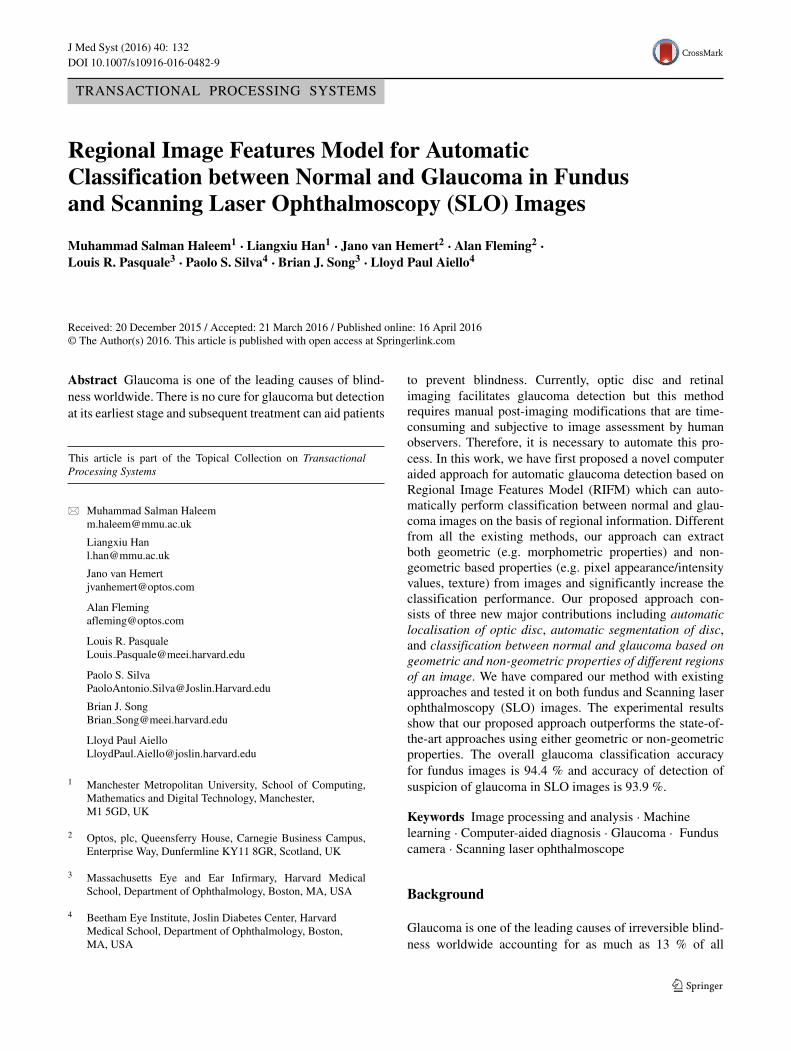
Fig. 4 Elaboration of optic disc image after image convolution witha Gaussian filter with a original image, b red channel convolutionat σ=2, c green channel convolution at σ = 2 and d red channelconvolution at σ = 8

Regional image features model

After optic disc segmentation, we need to determineRegional Image Feature Model (RIFM). Here we haveperformed the following steps:

Determination of regions in the optic disc cropped image

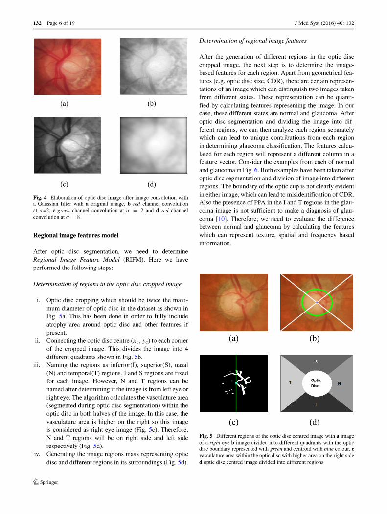
i. Optic disc cropping which should be twice the maxi-mum diameter of optic disc in the dataset as shown inFig. 5a. This has been done in order to fully includeatrophy area around optic disc and other features ifpresent.

ii. Connecting the optic disc centre (xc, yc) to each cornerof the cropped image. This divides the image into 4different quadrants shown in Fig. 5b.

iii. Naming the regions as inferior(I), superior(S), nasal(N) and temporal(T) regions. I and S regions are fixedfor each image. However, N and T regions can benamed after determining if the image is from left eye orright eye. The algorithm calculates the vasculature area(segmented during optic disc segmentation) within theoptic disc in both halves of the image. In this case, thevasculature area is higher on the right so this imageis considered as right eye image (Fig. 5c). Therefore,N and T regions will be on right side and left siderespectively (Fig. 5d).

iv. Generating the image regions mask representing opticdisc and different regions in its surroundings (Fig. 5d).

Determination of regional image features

After the generation of different regions in the optic disccropped image, the next step is to determine the image-based features for each region. Apart from geometrical fea-tures (e.g. optic disc size, CDR), there are certain represen-tations of an image which can distinguish two images takenfrom different states. These representation can be quanti-fied by calculating features representing the image. In ourcase, these different states are normal and glaucoma. Afteroptic disc segmentation and dividing the image into dif-ferent regions, we can then analyze each region separatelywhich can lead to unique contributions from each regionin determining glaucoma classification. The features calcu-lated for each region will represent a different column in afeature vector. Consider the examples from each of normaland glaucoma in Fig. 6. Both examples have been taken afteroptic disc segmentation and division of image into differentregions. The boundary of the optic cup is not clearly evidentin either image, which can lead to misidentification of CDR.Also the presence of PPA in the I and T regions in the glau-coma image is not sufficient to make a diagnosis of glau-coma [10]. Therefore, we need to evaluate the differencebetween normal and glaucoma by calculating the featureswhich can represent texture, spatial and frequency basedinformation.

(a) (b)

(c) (d)Fig. 5 Different regions of the optic disc centred image with a imageof a right eye b image divided into different quadrants with the opticdisc boundary represented with green and centroid with blue colour, cvasculature area within the optic disc with higher area on the right sided optic disc centred image divided into different regions

J Med Syst (2016) 40: 132 Page 7 of 19 132

(a) (b)Fig. 6 Comparison of a normal and b glaucoma images after divisionof optic disc cropped image into different regions

For each region, we have generated the feature matrix onthe basis of different features as follows:

FM =[FM

dgRG FM

texoffRG FM texscale

RG FMgRGFM

gabRG FMwav

RG

]

(6)

where RG represents red and green channel respectively,texoff represents textural features with variable offset val-ues, texscale represent textural features with variable scale,dg, g, wav and gab represent dyadic Gaussian, gradient fea-tures, wavelet features and gabor filter features. The detailsof each feature type are described below:

Gaussian features The mean value of each region afterconvolving the image with each Gaussian filter and its firstand second order derivatives determined for optic disc seg-mentation has been calculated to generate FM

gRG. We have

6 gaussian filters convolved at scales σ=2,4,8,16 for redand green channels and region which makes the length ofFM

gRG equal to 240.

Textural features Textural features can be determined byevaluating Grey Level Co-occurrence Matrix (GLCM) [31,32]. GLCM determines how often a pixel of a grey scalevalue i occurs adjacent to a pixel of the value j . The pixeladjacency can be observed in four different angles i.e. θ =0◦, 45◦, 90◦, 135◦. For the region of size p x q, we performsecond order textural analysis by constructing the GLCM(Cd(i, j)) and probability of pixel adjacency (Pd(i, j)) as:

Cd(i, j) ={

(p, q), (p + �x, q + �y) :I (p, q) = i, I (p + �x, q + �y) = j

Pd(i, j) = Cd(i,j)∑i

∑j Cd(i,j)

(7)

where �x and �y are offset values. The dimensions p

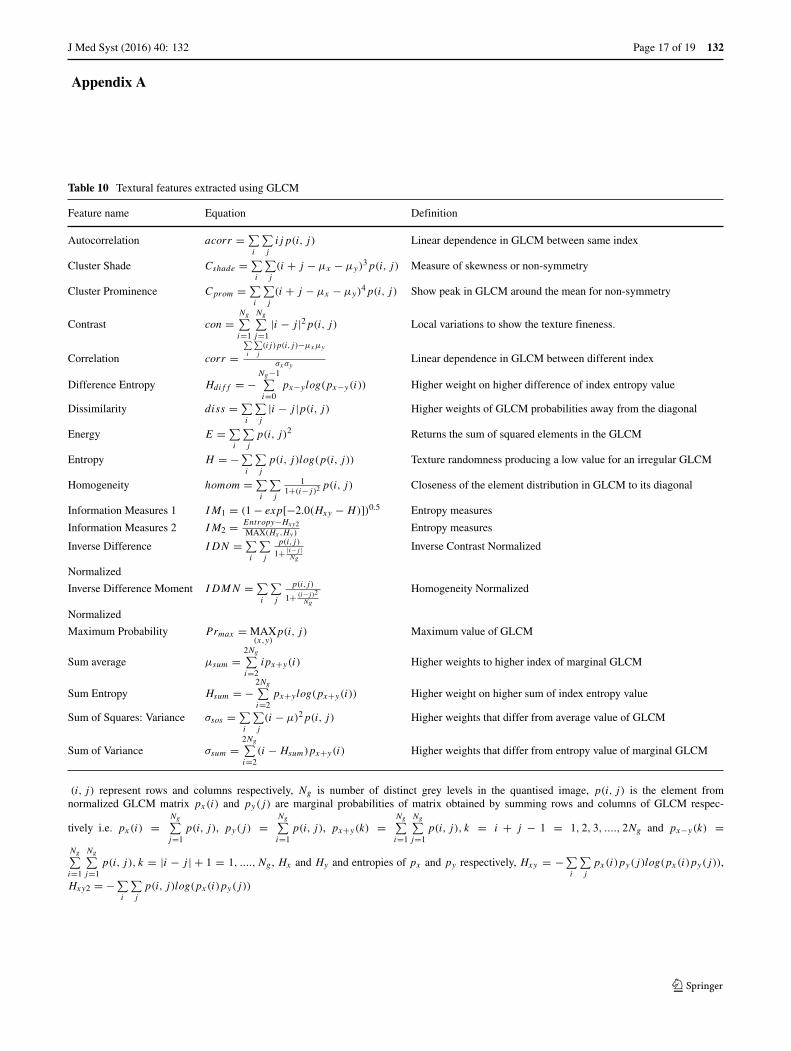
and q represent the bounding box of the particular regionamong I,S,N,T and OD. We have evaluated 20 features rep-resenting textural information which are enlisted in Table10 [33]. Since we have significantly large size of regions,the pixel adjacency can be evaluated at different offset

values �x and �y. We have varied these values rangingfrom 1 to 10 for both �x and �y to generate FM

texoffRG . We

have evaluated 20 textural features for each red and greenchannel (blue channel is set to zero in SLO so we did notcalculated for fundus images as well).

Apart from varying the offset values, we have also calcu-lated these features by convolving the image with Gaussianfilter at different scales σ=2,4,8,16 after fixing offset valuesat 1 for generating FM texscale

RG .

Dyadic gaussian features The Dyadic Gaussian featuresinvolve the downsampling of the optic disc cropped imageat multiple spatial scales [34, 35]. The calculation of abso-lute difference at different spatial scales can lead to thedevelopment of low-level visual ‘feature channels’ whichcan discriminate between normal and glaucoma images.We can generate certain features from red channel, greenchannel and combinations of both channels. The blue chan-nel is set to zero for SLO therefore we do not take thisinto account for fundus images as well. Apart from Red(R)and Green(G) channels, we have determined the featurechannels as follows:

Imn = (R+G)2

Yrg = R + G − 2|R − G| (8)

where Imn is the mean response of the both channels andthe Yrg shows their mixed response i.e. yellow channel.The absolute difference of the particular feature channelsat different spatial scales lead to determination of excita-tion and inhibition response. For determination of excitationand inhibition response, we have centre levels c and sur-round levels s of the spatial scales respectively. This can becalculated as:

Imn(c, s) = |Imn(c) − Interps−cImn(s)|RG(c, s) = |(R(c) − G(c)) − Interps−c(R(s) − G(s))|Yrg(c, s) = |(Yrg(c)) − Interps−c(Yrg(s))|

(9)

where Interps−c represent interpolation to s −c level. Notethat s=c+d. If we calculate mean response of each regioni.e. FM

dgRG=[I(c,s),RG(c,s),BY(c,s)]:

I reg(c, s) =N∑

i

I (c,s,n)N

RGreg(c, s) =N∑

i

RG(c,s,n)N

BY reg(c, s) =N∑

i

BY (c,s,n)N

(10)

whereN is number of pixels in the region. The dyadic Gaus-sian features can excite the optic disc region while inhibitingthe regions in its surroundings. For the case of glaucoma,the excited optic disc region can have higher intensity val-ues due large optic cup size while inhibition of atrophy

132 Page 8 of 19 J Med Syst (2016) 40: 132

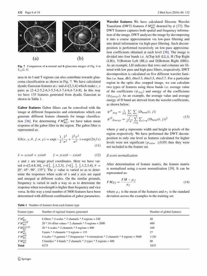
(a) (b)Fig. 7 Comparison of a normal and b glaucoma images of Fig. 6 atYrg(2, 5)

area in its I and T regions can also contribute towards glau-coma classification as shown in Fig. 7. We have calculateddyadic Gaussian features at c and d=[2,3,4] which make c, s

pairs as [2-4,2-5,2-6,3-5,3-6,3-7,4-6,4-7,4-8]. In this waywe have 135 features generated from dyadic Gaussian asshown in Table 1.

Gabor features Gabor filters can be convolved with theimage at different frequencies and orientations which cangenerate different feature channels for image classifica-tion [36]. For determining FM

gabRG , we have taken mean

response of the gabor filter in the region. The gabor filter isrepresented as:

Gb(x, y, θ, f, σ, γ ) = exp(−1

2(x2

σ 2+ y2γ 2

σ 2)∗ exp(i2πf x)

(11)

x = xcosθ + ysinθ y = ycosθ − xsinθ (12)

x and y are image pixel coordinates. Here we have var-ied σ=[2,4,8,16], γ=[13 ,

12 ,1,2,3], f =[14 ,

13 ,

12 ,1,2,3,4], θ =

[0◦, 45◦, 90◦, 135◦]. The γ value is varied so as to deter-mine the responses when scale of x and y axis are equaland unequal at different scales. On the similar grounds,frequency is varied in such a way so as to determine theresponse when wavelength is higher than frequency and viceversa. In this way a total number of 5600 features have beendetermined with different combination of gabor parameters.

Wavelet features We have calculated Discrete WaveletTransform (DWT) features FMwav

RG denoted by ψ [37]. TheDWT features captures both spatial and frequency informa-tion of the image. DWT analyses the image by decomposingit into a coarse approximation via low-pass filtering andinto detail information via high-pass filtering. Such decom-position is performed recursively on low-pass approxima-tion coefficients obtained at each level [38]. The image isdivided into four bands i.e. A(Top left (LL)), H (Top Right(LH)), V(Bottom Left (HL)) and D(Bottom Right (HH)).As an example, LH indicates that rows and columns are fil-tered with low pass and high pass filters, respectively. DWTdecomposition is calculated on five different wavelet fami-lies i.e. haar, db3, rbio3.3, rbio3.5, rbio3.7. For a particularregion in the optic disc cropped image, we can calculatetwo types of features using these bands i.e. average valueof the coefficients (ψAvg) and energy of the coefficients(ψEnergy). As an example, the average value and averageenergy of D band are derived from the wavelet coefficients,as shown below;

ψDAvg = 1

p q

∑

i=p

∑

j=q

|Dband(i, j)|ψD

Energy = 1p2 q2

∑

i=p

∑j=q(Dband(i, j))2

(13)

where p and q represents width and height in pixels of theregion respectively. We have performed the DWT decom-position to only one level as features calculated for higherlevels were not significant (pvalue ≥0.05) thus they werenot included in the feature set.

Z-score normalization

After determination of feature matrix, the feature matrixis normalized using z-score normalization [39]. It can berepresented as:

FMZS = FM − μf

σf

(14)

where μf is the mean of the features and σf is the standarddeviation across the examples in the training set.

Table 1 Number of features from each feature type

Feature types Number of regional features generated Number of global features

FMgRG 6 filters * 4 scales * 2 channels * 5 regions = 240 48

FMtexoffRG 20 * 10 offset values * 2 channels * 5 regions = 2000 400

FM texscaleRG 20 * 4 scales * 2 channels * 5 regions = 800 160

FMdgRG 9 pairs * 3 channels * 5 regions = 135 27

FMgabRG 4 scales * 5 gamma * 7 frequencies * 4 orientations * 2 channels * 5 regions = 5600 1120

FMwavRG 5 families * 4 bands * 2 channels * 2 types * 5 regions = 400 80

Total 9175 1835

J Med Syst (2016) 40: 132 Page 9 of 19 132

Fig. 8 Percentage of significantfeatures selected from eachcategory

05

101520253035404550

TexturalFeatures

Variable Offset

TexturalFeaturesVariable Scale

Gaussian DyadicGaussian

Wavelet Gabor

Perc

enta

ge o

f sig

nific

ant f

eatu

res

from

eac

h fe

atur

e ty

peFundus Regional Fundus Whole Image SLO Regional SLO Whole Image

Feature selection

Due to division of optic disc cropped images into fiveregions, the number of features generated is five times largerthan the situations where features are generated for a wholeimage. Since the determination of classifier constructedon such a high dimension of features is not computation-ally efficient and also some of these features may lead todepreciation of classifier performance, we have selectedthe features based on pvalue which are statistically sig-nificant (pvalue ≤0.05) towards glaucoma classification.Table 1 shows the number of features generated by eachfeature type whereas the percentage of features selectedfrom each feature type has been shown in Fig. 8. For fun-dus images, 2201 regional features out of 9175 featureshave been significant towards glaucoma classification and2836 regional features have been significant towards clas-sification in SLO images. The bar plot shows that thetextural and gabor features can be more clinically signif-icant compared to other types of features. Figure 8 andTable 1 also provides information regarding the total fea-tures generated and number of significant features selectedfor global features (whole image features) for comparisonpurpose.

After selection of relevant features, the feature dimen-sion is still high for classifier construction. In order toselect features most relevant towards classification, we haveperformed feature selection on significant feature set. Inour case, we have adopted wrapper feature selection [40].The wrapper feature selection is an iterative procedure ofmaximizing classification performance. In the feature selec-tion procedure, initially the data is divided into k folds(in our case k=5). Then the first feature is selected whichhas maximum mean classification performance across thefolds. During the next iterations, the features together with

previously selected features result in highest mean classi-fication performance are selected. This process continuesuntil there is little or no maximization towards classifica-tion performance. This process is in contrast to the filterselection approach [41] in which the feature ranking isperformed according to individual evaluation performanceof each feature. The individual evaluation performance isquantified according to their classification power and thefeatures beyond certain threshold value are selected forclassifier construction. However, our recent study [33] hasshown that features selected by wrapper feature selectionprocedure outperforms filter feature selection despite thefact that filter selection approach selects the best fea-tures from the pool whereas wrapper feature selectiondoes not necessarily follow the similar approach. Never-theless, the wrapper feature selection approach has beenperformed on the features which have been filtered out withpvalue ≤0.05.

For quantification of classification performance of thewrapper feature selection, we have certain performancemeasures such as Area Under the Curve (AUC), linearclassification accuracy and quadratic classification accu-racy. The AUC can be quantified by determining the areaunder Receiving Operating Characteristics (ROC). ROC isa graphical plot that illustrates the performance of a binaryclassifier system by area under it as it is created by plottingthe true positive rate against the false positive rate at vari-ous threshold settings [39]. The ROC curve of the selectedregional image features has been shown in Fig. 12 with a redplot. The wrapper feature selection by maximizing AUC istermed as ‘wrapper-AUC’. On the other hand, linear classi-fication accuracy is based on Linear Discriminant Analysis(LDA) by maximizing the distance between classes whileminimizing the variance within each class. Quadratic Dis-criminant Analysis (QDA) works on similar principle as

132 Page 10 of 19 J Med Syst (2016) 40: 132

Table 2 Comparison of number of features selected by each feature selection methods from different regions and total number of features selected

RIMONE SLO images

Regions Wrapper-AUC Wrapper-LDA Wrapper-QDA Wrapper-AUC Wrapper-LDA Wrapper-QDA

I 4 1 3 4 3 3

S 1 4 3 1 3 2

N 0 0 1 2 5 3

T 2 0 1 2 0 2

OD 4 2 1 2 0 0

Total 11 7 9 11 11 10

its linear counterpart except the classification boundarybetween classes is not linear and covariance matrix maynot be identically equal for each class. The wrapper fea-ture selection by maximizing LDA and QDA are termed as‘wrapper-LDA’ and ‘wrapper-QDA’ respectively.

We have run the wrapper feature selection with the per-formance measures mentioned previously on the significantfeatures. The number of features selected based on differ-ent feature selection methods (wrapper-AUC, wrapper-LDAand wrapper-QDA) is shown in Table 2. For example, forRIMONE dataset, when using wrapper-AUC, the total num-ber of regional features selected is 11. The total number offeature selected for wrapper-LDA and wrapper-QDA is 7and 9 respectively. The results of feature selection proce-dure have been shown in Fig. 9. The results shows that ifthe features are selected by AUC as performance measureof wrapper feature selection, we can achieve significantlyhigher classification accuracy compared to other perfor-mance measures. Also the classification power of regionalfeatures have been significantly better compared to globalfeatures both in case of fundus and SLO images. Moreover,the results in Table 2 shows that apart from the optic discregion, the other regions (such as I) can also play signif-icant role in glaucoma classification. The list of featuresselected after wrapper feature selection for both fundus andSLO images have been shown in Table 3. The list has mostlybeen dominated by either textural or Gabor features. As areference, HOD

diff G(2) is the ‘Difference Entropy’ from Table10 where OD in superscript represent the optic disc region,G in subscript represent the green channel where as 2 insubscript represent the offset value. If the number is not insubscript (as in case of corrOD

G (2)), then it represent thescale (σ ) value.

Classifier setting

On selected regional image features, we have constructedthe binary classifier for glaucoma classification usingSupport Vector Machines (SVM) [42]. In recent studies[43], non-parallel SVM has performed better compared

to traditional SVM methods. In traditional SVM, twoparallel planes are generated such that each plane is as farapart as possible however in non-parallel SVM, the condi-tion of parallelism is dropped. Among non-parallel SVM,

2 4 6 8 10 120.7

0.75

0.8

0.85

0.9

0.95

1

Number of Features Selected

Mea

n C

lass

ifica

tion

Per

form

ance

AUC Regional

LDA Regional

QDA Regional

AUC whole

LDA whole

QDA whole

(a)

2 4 6 8 10 120.7

0.75

0.8

0.85

0.9

Number of Features Selected

Mea

n C

lass

ifica

tion

Per

form

ance

AUC Regional

LDA Regional

QDA Regional

AUC whole

LDA whole

QDA whole

(b)

Fig. 9 Feature selection procedure for both regional and whole imagefeatures in different classification performance

J Med Syst (2016) 40: 132 Page 11 of 19 132

Table 3 Symbols of features selected by sequential maximization approach. These features also represent the x-axis of Fig. 9

Criteria Fundus image SLO images

Regional Features

AUC HODdiff G(2), Y

Irg(2, 6), GbT

G(45◦, 0.5, 4, 0.5),corrODG (2), I I

mn(2, 5), YIrg(2, 5), PrN

Rmax(1), GbODG (135◦, 4, 2, 0.5),

IMI1R(2) GbOD

G (45◦, 0.5, 4, 0.5), GbIG(0◦, 0.5, 8, 0.33), GbOD

R (0◦, 1, 2, 3), HSsumR(7), GbT

R(45◦, 4, 16, 2),HS

diff R(6), GbIR(90◦, 4, 16, 1), IMT

1R(2), GbODG (90◦, 2, 16, 3), GbI

R(135◦, 3, 4, 0.5), HIsumR(10),

GbODR (0◦, 0.33, 4, 1) GbT

R(0◦, 0.5, 2, 2)

LDA CSshadeG(2), IMI

1R(2), IMS2R(2), CS

shadeG(10), ISmn(3, 7), RGI (2, 5), ES

R(3),GbNG(0◦, 3, 2, 1), μN

sumG(1),

IMOD1G (16), IMOD

1G(4), GbODR (135◦, 1, 8, 3) ES

R(1), IMI2R(4), H

Ndiff R(10), μ

NsumG(2), C

NpromG(1),

HIdiff G(2)

QDA ESR(7), GbI

G(45◦, 1, 4, 1), corrIR(4), BYOD(4, 8), IS

mn(3, 7), RGI (2, 6), GbTR(0◦, 0.5, 4, 0.33), HS

diff G(8),

HSsumR(6), GbN

R (0◦, 1, 4, 0.5), GbSG(135◦, 2, 2, 1), GbT

R(45◦, 4, 2, 1), GbNR (45◦, 4, 2, 1), corrT

R(1), EIG(8),

CTshadeG(9), GbI

G(0◦, 3, 16, 1) conN(9)G ,NN

xxG(8)

Whole Image Features

AUC IM1G(2), IM1R(8), CpromG(10), GbR(135◦, 0.33, 8, 0.5), IM1G(8), ψHRAvg(db3), ψH

RAvg(rbio3.7), IM1G(1),

CpromR(6), CpromG(6) conG(8), HG(4), Hdiff G(4), GbG(135◦, 0.5, 16, 0.33),IM1R(16), GbG(90◦, 2, 8, 0.33)

LDA IM1G(8), GbR(45◦, 4, 2, 1), GbG(135◦, 2, 16, 1), ER(9), IM1G(8), RG(4, 8), IM1G(8), acorrG(1), ψDGAvg(db3),

homomR(8) RG(3, 7), σsosG(4), GbG(90◦, 4, 4, 0.5), GbG(45◦, 2, 4, 0.5),RG(3, 7), σsosG(3), ER(8)

QDA IM1G(8), IDNG(16), GbR(135◦, 0.33, 8, 0.5), dissG(4), IM1G(8), Hdiff G(2), homomG(3), conG(9)

ψDREnergy(haar)

Twin SVM has performed better compared to its other coun-terparts [44]. Mathematically, the Twin SVM is constructedby solving two quadratic programming problems

minws1,bs1,qs12 (Xs1ws1+ε1bs1)

T (Xs1ws1+ε2bs1) + C1ε1q

s.t. − (Xs2ws1 + ε2bs1) + q ≥ ε2, q ≥ 0

(15)

minws2,bs2,qs12 (Xs2ws2+ε1bs2)

T (Xs2ws2+ε2bs2)+C2ε1q

s.t. − (Xs1ws2 + ε1bs2) + q ≥ ε1, q ≥ 0

(16)

The performance of Twin SVM has been compared withtraditional SVM. The traditional SVM classifier can beexpressed as:

maxα≥0∑

i

αi − 12

∑

j,k

αjαkyjykk(xj , xk)

subject to0 ≤ αi ≤ C and∑

i

αiyi = 0(17)

where C is the penalty term. k(xi, x) represents the ker-nel function. In linear SVM case, k(xj , xk) = xj .xk . Thekernel function in Eq. 17 can be replaced for developingnon-linear SVM classifier such as Radial Based Function,polynomial and sigmoid SVM. The k(xj , xk) in Eq. 17 isreplaced with gaussian kernel mentioned as: k(xi, x) =

Table 4 Input parameters for the classifiers

Classifier type Parameter values

Twin SVM C1=6, C2 = 6.14, ε1=0.2, ε2=0.1

Linear SVM C = 4

Polyniomial SVM = 0.9, d = 1, C = 1

RBF SVM = 0.05, C = 4

Sigmoid SVM = 0.05, coeff 0 = 1, C = 1

132 Page 12 of 19 J Med Syst (2016) 40: 132

(a) (b)

(c) (d)Fig. 10 Examples of optic disc segmentation using proposedapproach a,b are examples from RIM-ONE and c,d are examples fromSLO images. The red outline shows the original annotation aroundoptic disc whereas the green outline shows the automatic annotationsfrom proposed approach

exp(−||xi − x||2). In polynomial function the k(xj , xk) =(xj .xk)

d and in sigmoid SVM k(xj , xk) = tanh(xj .xk +coeff 0), where coeff 0 is sigmoid coefficient. We havetested different paremeters on libsvm [42] on C-SVC foreach kernel function parameters and cost value. We havetested different parameter values for these classifiers and thevalues for which the respective SVM classifier performedthe best in both fundus and SLO images have been shownin Table 4.

Apart from SVM classifiers, we have also compared thepeformance with LDA and QDA as they have also beeninvolved in the feature selection process

Experimental evaluation and discussion

Evaluation metrics

For optic disc segmentation performance, we have DiceCoefficient [45] as an evaluation measurement, which is thedegree of overlap of two regions. It is defined as:

D(A, B) = 2|A ∩ B||A ∪ B| , (18)

where A and B are the segmented regions surrounded bymodel boundary and annotations from the ophthalmologistsrespectively, ∩ denotes the intersection and ∪ denotes theunion. Its value varies between 0 and 1 where a higher value,indicates an increased degree of overlap. Apart from thatwe have adopted standard evaluation metrics using accuracy(Acc), sensitivity (Sn or true positive rate) and specificity(Sp or false positive rate) described as follows:

Acc = T N+T PT N+T P+FN+FP

Sn = T PT P+FN

Sp = T NT N+FP

(19)

where T P, T N, FP and FN are true positives, true neg-atives, false positives and false negatives respectively. Thesignificance of the improvement of the classification accu-racy has been evaluated by McNemar’s test [46]. TheMcNemar’s test can be used to compare classificationresults across different methods and can generate Chi-squared value as:

χ2 = (|c1err − c2err | − 1)2

c1err + c2err

(20)

where c1err and c2err are the number of images misclassi-fied by different methods. We have compared the classifica-tion performance of RIFM model to the geometric methodsas well as non-geometric methods. The Chi-squared valuegenerated is then converted to pvalue for testing statistical

(a) (b)

(c)Fig. 11 Comparison of optic disc segmentation of proposed approachwith previous methods a Active Shape Model [48], b Chan-Vese [49]and c the proposed approach

J Med Syst (2016) 40: 132 Page 13 of 19 132

Table 5 Accuracy comparison of the proposed optic disc segmentation approach with our previous approach

RIM-ONE SLO images

Normal Glaucoma Both Normal Glaucoma Both

The Proposed Approach 0.95 ± 0.03 0.92 ± 0.07 0.94 ± 0.05 0.91 ± 0.07 0.89 ± 0.07 0.90 ± 0.07

Active Shape Model 0.91 ± 0.06 0.87 ± 0.09 0.89 ± 0.06 0.82 ± 0.10 0.80 ± 0.08 0.81 ± 0.09

Chan-Vese Model 0.92 ± 0.06 0.84 ± 0.12 0.89 ± 0.07 0.85 ± 0.10 0.82 ± 0.12 0.84 ± 0.10

significance of the improvement. The test is considered sta-tistically significant if the pvalue is below certain value. Typ-ical standard values are 0.1, 0.05 and 0.01 (χ2 = 2.706,3.841and 6.635 respectively).

Accuracy comparison with the state-of-the-artapproaches

We have conducted experimental evaluation on both fundusand SLO image datasets from three aspects:

1) Optic disc segmentation accuracy performance.2) Accuracy performance based on different classification

algorithms and feature selection methods.3) Accuracy performance comparison with either geomet-

ric or non-geometric methods.

The image datasets used for the evaluation are describedin “Datasets used for experimentation”, consisting of a rep-resentative and heterogeneous image dataset including bothfundus and SLO images totalling 189 images; 124 from fun-dus dataset and 65 from SLO dataset. Each of the fundus andSLO dataset has been split into cross-validation sets and thetest sets. In the cross-validation sets, N-fold cross validation[12] has been performed for classification model validation.

The essence of n-fold cross validation is to randomly dividea dataset into n equal sized subsets and of the n subsets, asingle subset is retained as the validation data for testing themodel, and the remaining n-1 subsets are used as trainingdata. The cross-validation process is then repeated n times(the folds), with each of the n subsamples used exactly onceas the validation data. The cross-validation accuracy hasbeen determined after training the classifier on n-1 subsetsand testing on the nth subset. This has been performed foreach subset in the cross-validation set. The cross-validationsets for classifier training are different from that of featureselection process. The accuracy on the test sets for eachdataset are then calculated after training the classifier onthe images of cross-validation sets of the respective dataset.Additionally, to address dataset imbalance, the EnsembleRandom Under Sampling (ERUS) is used, in which usefulsamples can be selected for learning classifiers [47].

Optic disc segmentation accuracy performance

We have compared our segmentation methods with clini-cal annotations and existing models such as Active ShapeModel [48], Chan-Vese [49]. The experimental results areshown in Figs. 10 and 11 and our method outperformsthe existing methods. The mean and standard deviation

Table 6 Comparison of classification accuracies across different feature selection methods in cross-validation set

RIMONE SLO images

Classifier wrap-AUC wrap-LDA wrap-QDA wrap-AUC wrap-LDA wrap-QDA

Twin SVM 96.3 % 90.0 % 78.8 % 94.1 % 84.3 % 78.4 %

Linear SVM 95.0 % 90.0 % 81.3 % 94.1 % 84.3 % 78.4 %

Polynomial SVM 95.0 % 90.0 % 81.3 % 94.1 % 84.3 % 78.4 %

RBF SVM 90.0 % 87.5 % 82.5 % 82.3 % 78.4 % 82.3 %

Sigmoid SVM 78.8 % 92.5 % 77.5 % 78.4 % 74.5 % 78.4 %

LDA 95.0 % 88.8 % 80.0 % 90.5 % 82.4 % 78.4 %

QDA 85.0 % 81.3 % 86.3 % 78.4 % 68.6 % 82.4 %

132 Page 14 of 19 J Med Syst (2016) 40: 132

Table 7 Comparison of classification accuracies across different feature selection methods in test set

RIMONE SLO images

Classifier wrap-AUC wrap-LDA wrap-QDA wrap-AUC wrap-LDA wrap-QDA

Twin SVM 90.9 % 86.4 % 81.8 % 85.7 % 78.6 % 64.3 %

Linear SVM 90.9 % 88.6 % 81.8 % 78.6 % 71.4 % 64.3 %

Polynomial SVM 90.9 % 88.6 % 81.8 % 78.6 % 71.4 % 64.3 %

RBF SVM 88.6 % 86.4 % 97.7 % 78.6 % 57.1 % 78.6 %

Sigmoid SVM 84.1 % 86.4 % 86.4 % 64.3 % 28.6 % 28.6 %

LDA 88.6 % 88.6 % 79.5 % 71.4 % 71.4 % 64.3 %

QDA 86.4 % 88.6 % 90.9 % 64.3 % 35.7 % 74.1 %

of Dice Coefficients of our previous approach [20] andproposed approach has been evaluated on both RIM-ONEand SLO datasets with respect to both healthy and glau-comatous images as shown in Table 5. Also some of theexamples of optic disc segmentation compared to clinicalannotations has been shown in Fig. 10. The visual resultsshow that segmentation accuracy is quite comparable toclinical annotation; especially in the right column whichrepresent the examples of glaucomatous optic disc withPPA.

Accuracy comparison based on different classificationalgorithms and feature selection methods

The performance of regional features selected under theproposed approach compared with other regional featureselection methods across different classifiers have beenpresented in Table 6 for cross-validation sets and inTable 7 for the test-sets. According to the results, thefeature sets selected by AUC maximization have higheraccuracy on both cross-validation sets and the test sets com-pared to the ones selected by maximization of linear and

quadratic classification accuracy. The results also showthat dropping the parallelization condition from the SVMcan have marginal improvement in terms of classificationaccuracy; like in case of Twin SVM. Moreover, classi-fier with linear specifications i.e. Linear SVM and LDAhave performed significantly better compared to other non-linear counterparts. The performance of Polynomial SVMis comparable to Linear SVM however, it has achieved thisaccuracy at degree d = 1 which is the special case oflinear classification. The performance of the classifiers oncross-validation sets and the test sets have been combinedand detailed in Table 8. In Table 8, we have compared theclassifier performance with respect to sensitivity and speci-ficity along with classification accuracy. We have identifiedthe best results of each classifier across different featuresets mentioned in Table 6. For example, Twin SVM hasthe best results on wrapper-AUC or RBF-SVM has thebest results on wrapper-QDA so they are the best featureset for the respective classifiers. The results show that thenon-linear classifiers such as RBF-SVM and QDA havehigh false negatives compared to their linear counterpartswhich have resulted the depreciation in their performance.

Table 8 Comparison of sensitivity, specificity and accuracy across different classifiers

RIMONE SLO images

Classifier TP FN TN FP Sn Sp Acc TP FN TN FP Sn Sp Acc

Twin SVM 36 3 81 4 92.3 % 95.3 % 94.4 % 17 2 43 4 89.5 % 93.5 % 93.9 %

Linear SVM 36 3 80 5 92.3 % 94.1 % 93.5 % 17 2 42 4 89.5 % 91.3 % 90.8 %

Polynomial SVM 36 3 80 5 92.3 % 94.1 % 93.5 % 18 1 41 5 94.7 % 89.1 % 90.8 %

RBF-SVM 31 8 80 5 79.5 % 94.1 % 89.5 % 14 5 39 7 73.7 % 86.7 % 81.5 %

Sigmoid SVM 32 7 80 5 82.1 % 94.1 % 90.3 % 15 4 34 12 78.9 % 73.9 % 75.4 %

LDA 36 3 79 6 92.3 % 92.9 % 92.7 % 14 5 38 8 73.7 % 82.6 % 80.0 %

QDA 30 9 78 7 76.9 % 91.8 % 87.1 % 10 9 42 4 52.6 % 91.3 % 80.0 %

J Med Syst (2016) 40: 132 Page 15 of 19 132

0 0.2 0.4 0.6 0.8 10

0.1

0.2

0.3

0.4

0.5

0.6

0.7

0.8

0.9

1

False Positive Rate (1−Specificity)

True

Pos

itive

Rat

e (S

ensi

tivity

)

Regional Features AUC:0.96371Global Features AUC:0.93929Vertical CDR AUC:0.88471Horizontal CDR AUCC:0.86256Vasculature Shift AUC:0.83506

(a)

0 0.2 0.4 0.6 0.8 10

0.1

0.2

0.3

0.4

0.5

0.6

0.7

0.8

0.9

1

False Positive Rate (1−Specificity)

True

Pos

itive

Rat

e (S

ensi

tivity

)

Regional Features AUC:0.97204Global Features AUC:0.91612Vertical CDR AUC:0.95559Horizontal CDR AUCC:0.85362Vasculature Shift AUC:0.65296

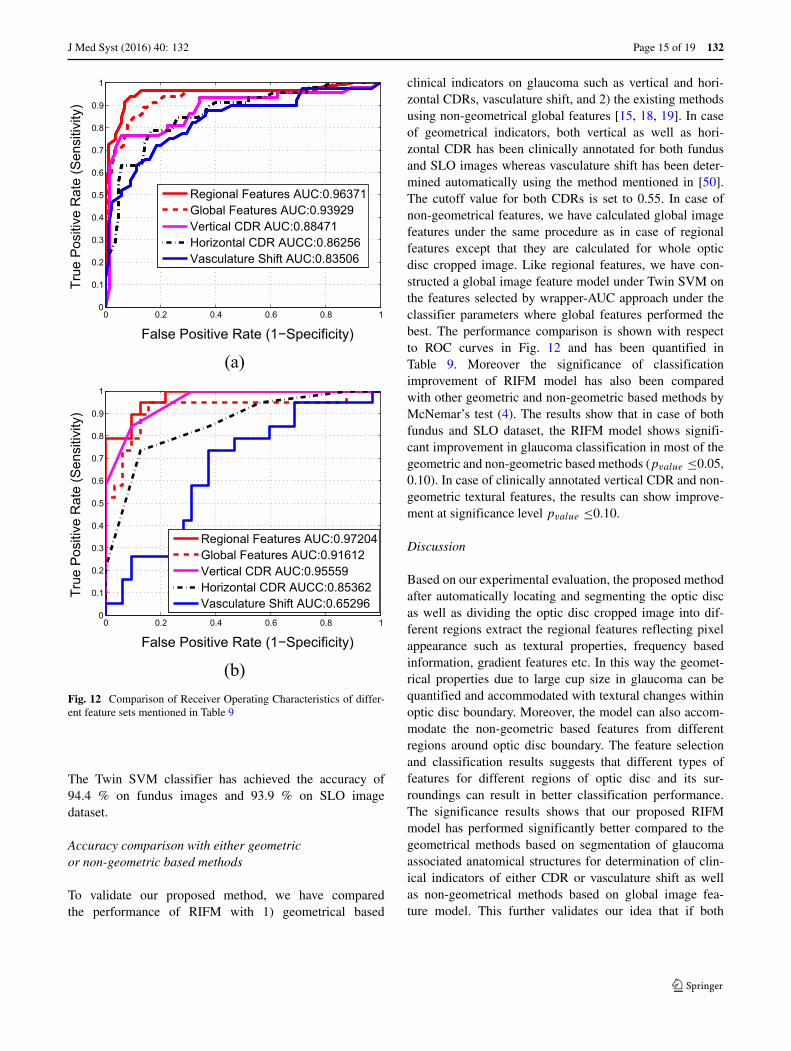
(b)Fig. 12 Comparison of Receiver Operating Characteristics of differ-ent feature sets mentioned in Table 9

The Twin SVM classifier has achieved the accuracy of94.4 % on fundus images and 93.9 % on SLO imagedataset.

Accuracy comparison with either geometricor non-geometric based methods

To validate our proposed method, we have comparedthe performance of RIFM with 1) geometrical based

clinical indicators on glaucoma such as vertical and hori-zontal CDRs, vasculature shift, and 2) the existing methodsusing non-geometrical global features [15, 18, 19]. In caseof geometrical indicators, both vertical as well as hori-zontal CDR has been clinically annotated for both fundusand SLO images whereas vasculature shift has been deter-mined automatically using the method mentioned in [50].The cutoff value for both CDRs is set to 0.55. In case ofnon-geometrical features, we have calculated global imagefeatures under the same procedure as in case of regionalfeatures except that they are calculated for whole opticdisc cropped image. Like regional features, we have con-structed a global image feature model under Twin SVM onthe features selected by wrapper-AUC approach under theclassifier parameters where global features performed thebest. The performance comparison is shown with respectto ROC curves in Fig. 12 and has been quantified inTable 9. Moreover the significance of classificationimprovement of RIFM model has also been comparedwith other geometric and non-geometric based methods byMcNemar’s test (4). The results show that in case of bothfundus and SLO dataset, the RIFM model shows signifi-cant improvement in glaucoma classification in most of thegeometric and non-geometric based methods (pvalue ≤0.05,0.10). In case of clinically annotated vertical CDR and non-geometric textural features, the results can show improve-ment at significance level pvalue ≤0.10.

Discussion

Based on our experimental evaluation, the proposed methodafter automatically locating and segmenting the optic discas well as dividing the optic disc cropped image into dif-ferent regions extract the regional features reflecting pixelappearance such as textural properties, frequency basedinformation, gradient features etc. In this way the geomet-rical properties due to large cup size in glaucoma can bequantified and accommodated with textural changes withinoptic disc boundary. Moreover, the model can also accom-modate the non-geometric based features from differentregions around optic disc boundary. The feature selectionand classification results suggests that different types offeatures for different regions of optic disc and its sur-roundings can result in better classification performance.The significance results shows that our proposed RIFMmodel has performed significantly better compared to thegeometrical methods based on segmentation of glaucomaassociated anatomical structures for determination of clin-ical indicators of either CDR or vasculature shift as wellas non-geometrical methods based on global image fea-ture model. This further validates our idea that if both

132 Page 16 of 19 J Med Syst (2016) 40: 132

Table 9 Accuracy comparison of the proposed RIFM model with either geometric or non-geometric-based methods

RIMONE SLO Images

Features (i.e. geometric or TP FN TN FP Sn Sp Acc pvalue TP FN TN FP Sn Sp Acc pvalue

non-geometric)

RIFM 36 3 81 4 92.3 % 95.3 % 94.4 % – 17 2 31 1 89.5 % 96.9 % 94.1 % –

Geometric based Methods

Geo-metric (Vertical CDR) 29 10 80 5 74.4 % 94.1 % 87.9 % <0.10 16 3 29 3 84.2 % 90.6 % 88.2 % =0.28

Geo-metric (Horizontal CDR) 26 13 76 9 66.7 % 89.4 % 82.3 % <0.01 14 5 28 4 73.7 % 87.5 % 82.4 % <0.10

Geo-metric (Vasculature Shift) 26 13 75 10 66.7 % 88.2 % 81.5 % <0.01 14 5 20 12 73.7 % 62.5 % 66.7 % <0.001

Non-geometric based Methods

Global Features (Mix) 35 4 74 11 89.7 % 87.1 % 87.9 % <0.10 13 6 28 4 68.4 % 87.5 % 80.4 % <0.10

Textural Features (Variable Offset) [18, 19] 30 9 71 14 76.9 % 83.5 % 81.5 % <0.01 11 8 18 12 57.9 % 56.2 % 56.9 % <0.001

Textural Features (Variable Scale) [18, 19] 35 4 74 11 89.7 % 87.1 % 87.9 % <0.10 12 7 21 11 63.2 % 65.6 % 64.7 % <0.005

Textural Features (Scale + Offset) [18, 19] 35 4 74 11 89.7 % 87.1 % 87.9 % <0.10 13 6 28 4 68.4 % 87.5 % 80.4 % <0.10

Higher Order Spectra Features [19] 34 5 74 11 87.2 % 87.1 % 87.1 % <0.05 12 7 24 8 63.2 % 75.0 % 70.6 % <0.01

Gabor Features [51] 34 5 75 10 87.2 % 88.2 % 87.9 % <0.10 11 8 24 8 57.9 % 75.0 % 68.6 % <0.01

Wavelet Features [15] 31 8 65 20 79.5 % 76.5 % 77.4 % <0.001 11 8 24 8 57.9 % 75.0 % 68.6 % <0.01

Gaussian Features 32 7 67 18 82.1 % 78.8 % 79.8 % <0.01 10 9 26 6 52.6 % 81.3 % 70.6 % <0.05

Dyadic Gaussian Features 28 11 75 10 71.8 % 88.2 % 83.1 % <0.05 10 9 26 6 52.6 % 81.3 % 70.6 % <0.05

geometrical and non-geometrical indications are combinedtogether, this can significantly increase the glaucoma clas-sification performance.

Conclusion

In this paper, we have proposed the novel computer-aidedapproach: Regional Image Features Model (RIFM) whichcan extract both geometric and non-geometric propertiesfrom an image and automatically perform classificationbetween normal and glaucoma images on the basis ofregional image information. The proposed method automat-ically localises and segments the optic disc, divides the opticdisc surroundings into different regions and performs glau-coma classification on the basis of image-based informationof different regions. The novelties of the work include 1) anew accurate method of automatic optic disc localisation; 2)a new accurate method of optic disc segmentation; 3) a newRIFM on extraction of both geometric and non-geometricproperties from different regions of optic disc and its sur-roundings for classification between normal and glaucomaimages.

The performance of our proposed RIFM model has beencompared across different feature sets, classifiers and pre-vious approaches and has been evaluated on on both fundusand SLO image datasets. The experimental evaluation resultshows our approach outperforms existing approaches using

either geometric or non-geometric approaches. The clas-sification accuracy on fundus and SLO images is 94.4 %and 93.9 % respectively. The results validate our hypoth-esis of combining both geometrical and non-geometricalindications since they are significantly better compared tomethods which are based on either geometrical or non-geometrical indications.

Further research is needed to test the model on datasetscomposed of healthy as well as various stages of glaucoma.Additionally, because the most common clinical indicatorfor glaucoma detection is to measure CDR value (based onmanual approaches), we will further develop the proposedRIFM approach for automated CDR measurement.

Acknowledgments This work is fully supported by EPSRC-DHPAfunded project Automatic Detection of Features in Retinal Imagingto Improve Diagnosis of Eye Diseases and Optos plc. (Grant Ref:EP/J50063X/1). Harvard Medical school provided SLO image dataand made contributions to data annotation and domain knowledge.Dr. Pasquale is supported by Harvard Medical School DistinguishedScholar Award. Dr. Song is supported by a departmental K12 grantfrom the NIH through the Harvard Vision Clinical Scientist Develop-ment Program with grant number 5K12EY016335.

Open Access This article is distributed under the terms of theCreative Commons Attribution 4.0 International License (http://creativecommons.org/licenses/by/4.0/), which permits unrestricteduse, distribution, and reproduction in any medium, provided you giveappropriate credit to the original author(s) and the source, provide alink to the Creative Commons license, and indicate if changes weremade.

J Med Syst (2016) 40: 132 Page 17 of 19 132

Appendix A

Table 10 Textural features extracted using GLCM

Feature name Equation Definition

Autocorrelation acorr = ∑

i

∑

j

ijp(i, j) Linear dependence in GLCM between same index

Cluster Shade Cshade = ∑

i

∑

j

(i + j − μx − μy)3p(i, j) Measure of skewness or non-symmetry

Cluster Prominence Cprom = ∑

i

∑

j

(i + j − μx − μy)4p(i, j) Show peak in GLCM around the mean for non-symmetry

Contrast con =Ng∑

i=1

Ng∑

j=1|i − j |2p(i, j) Local variations to show the texture fineness.

Correlation corr =∑

i

∑

j

(ij)p(i,j)−μxμy

σxσyLinear dependence in GLCM between different index

Difference Entropy Hdiff = −Ng−1∑

i=0px−y log(px−y(i)) Higher weight on higher difference of index entropy value

Dissimilarity diss = ∑

i

∑

j

|i − j |p(i, j) Higher weights of GLCM probabilities away from the diagonal

Energy E = ∑

i

∑

j

p(i, j)2 Returns the sum of squared elements in the GLCM

Entropy H = −∑

i

∑

j

p(i, j)log(p(i, j)) Texture randomness producing a low value for an irregular GLCM

Homogeneity homom = ∑

i

∑

j

11+(i−j)2

p(i, j) Closeness of the element distribution in GLCM to its diagonal

Information Measures 1 IM1 = (1 − exp[−2.0(Hxy − H)])0.5 Entropy measures

Information Measures 2 IM2 = Entropy−Hxy2MAX(Hx ,Hy)

Entropy measures

Inverse Difference IDN = ∑

i

∑

j

p(i,j)

1+ |i−j |Ng

Inverse Contrast Normalized

Normalized

Inverse Difference Moment IDMN = ∑

i

∑

j

p(i,j)

1+ (i−j)2Ng

Homogeneity Normalized

Normalized

Maximum Probability Prmax = MAX(x,y)

p(i, j) Maximum value of GLCM

Sum average μsum =2Ng∑

i=2ipx+y(i) Higher weights to higher index of marginal GLCM

Sum Entropy Hsum = −2Ng∑

i=2px+y log(px+y(i)) Higher weight on higher sum of index entropy value

Sum of Squares: Variance σsos = ∑

i

∑

j

(i − μ)2p(i, j) Higher weights that differ from average value of GLCM

Sum of Variance σsum =2Ng∑

i=2(i − Hsum)px+y(i) Higher weights that differ from entropy value of marginal GLCM

(i, j) represent rows and columns respectively, Ng is number of distinct grey levels in the quantised image, p(i, j) is the element fromnormalized GLCM matrix px(i) and py(j) are marginal probabilities of matrix obtained by summing rows and columns of GLCM respec-

tively i.e. px(i) =Ng∑

j=1p(i, j), py(j) =

Ng∑

i=1p(i, j), px+y(k) =

Ng∑

i=1

Ng∑

j=1p(i, j), k = i + j − 1 = 1, 2, 3, ...., 2Ng and px−y(k) =

Ng∑

i=1

Ng∑

j=1p(i, j), k = |i − j | + 1 = 1, ...., Ng , Hx and Hy and entropies of px and py respectively, Hxy = −∑

i

∑

j

px(i)py(j)log(px(i)py(j)),

Hxy2 = −∑

i

∑

j

p(i, j)log(px(i)py(j))

132 Page 18 of 19 J Med Syst (2016) 40: 132

References

1. Suzanne, R., The most common causes of blindness, 2011. http://www.livestrong.com/article/92727-common-causes-blindness.

2. Parekh, A., Tafreshi, A., Dorairaj, S., and Weinreb, R. N., Clini-cal applicability of the international classification of disease andrelated health problems (icd-9) glaucoma staging codes to pre-dict disease severity in patients with open-angle glaucoma. J.Glaucoma 23:e18–e22, 2014.

3. National Health Services UK, 2011. http://www.nhscareers.nhs.uk/features/2011/june/.

4. Tham, Y.-C., Li, X., Wong, T. Y., Quigley, H.A., Aung, T., andCheng, C.-Y., Global prevalence of glaucoma and projections ofglaucoma burden through. Ophthalmology 121(2014):2081–2090,2040.

5. Jonas, J., Budde, W., and Jonas, S., Ophthalmoscopic evaluationof optic nerve head. Surv. Ophthalmol. 43:293–320, 1999.

6. Williams, G., Scott, I., Haller, J., Maquire, A., Marcus, D.,and McDonald, H., Single-field fundus photography for dia-betic retinopathy screening: a report by the american academy ofophthalmology. Ophthamology 111:1055–1062, 2004.

7. Jelinek, H., and Cree, M., (Eds.), Automated Image Detection ofRetinal Pathology. Taylor and Francis Group. 2010.

8. Patton, N., Aslam, T.M., MacGillivray, T., Deary, I. J., Dhillon,B., Eikelboom, R.H., Yogesan, K., and Constabl, I., Retinal imageanalysis: Concepts, applications and potential. Prog. Retin. EyeRes. 25:99 127, 2005.

9. Budenz, D. L., Barton, K., Whiteside-de Vos, J., Schiffman, J.,Bandi, J., Nolan, W., Herndon, L., Kim, H., Hay-Smith, G., andTielsch, J.M., Prevalence of glaucoma in an urban west africanpopulation. JAMA Ophthalmol. 131:651–658, 2014.

10. Derick, R., Pasquale, L., Pease, M., and Quigley, H., A clinicalstudy of peripapillary crescents of the optic disc in chronic exper-imental glaucoma in monkey eyes. Arch. Ophthalmol. 112:846–850, 1994.

11. Nayak, J., Acharya, R., Bhat, P., Shetty, N., and Lim, T.-C., Auto-mated diagnosis of glaucoma using digital fundus images. J. Med.Syst. 33:337–346, 2009.

12. Smola, A., and Vishwanathan, S. Introduction to Machine Learn-ing: Cambridge University Press, 2008.

13. Haleem, M. S., Han, L., Hemert, J. v., and Li, B., Automaticextraction of retinal features from colour retinal images for glau-coma diagnosis: a review. Comput. Med. Imaging Graph. 37:581–596, 2013.

14. Bock, R., Meier, J., Nyul, L., Hornegger, J., and Michelson, G.,Glaucoma risk index:automated glaucoma detection from colorfundus images.Med. Image Anal. 14:471–481, 2010.

15. Dua, S., Acharya, U. R., Chowriappa, P., and Sree, S. V., Wavelet-based energy features for glaucomatous image classification.IEEE Trans. Inf. Technol. Biomed. 16:80–87, 2012.

16. Breiman, L. Random forests, Tech. rep. Berkeley: University ofCalifornia, 2001.

17. Keerthi, S., Shevade, S., Bhattacharyya, C., and Murthy, K.Improvements to platt’s smo algorithm for svm classifier design,Tech. rep.: National University of Singapore, 1998.

18. Acharya, R., Dua, S., Du, X., Sree, V., and Chua, C. K., Automateddiagnosis of glaucoma using texture and higher order spectrafeatures. IEEE Trans. Inf. Technol. Biomed. 15:449–455, 2011.

19. Noronhaa, K., Acharya, U., Nayak, K., Martis, R., and Bhandary,S., Automated classification of glaucoma stages using higher ordercumulant features. Biomed. Signal Process. Control 10:174–183,2014.

20. Haleem, M. S., Han, L., Li, B., Nisbet, A., Hemert, J. v., andVerhoek, M., Automatic extraction of optic disc boundary fordetecting retinal diseases. In: 14th IASTED International Confer-ence on Computer Graphics and Imaging (CGIM), 2013.

21. Optos, 2015. www.optos.com.22. Fumero, F., Alayon, S., Sanchez, J., Sigut, J., and Gonzalez-

Hernandez, M., Rim-one: An open retinal image database foroptic nerve evaluation. In: Proceedings of the 24th InternationalSymposium on Computer-BasedMedical Systems (CBMS), 2011.

23. Medical image analysis group. http://medimrg.webs.ull.es/research/retinal-imaging/rim-one/.

24. Mahfouz, A., and Fahmy, A. S., Fast localization of the optic discusing projection of image features. IEEE Trans. Image Process.19:3285–3289, 2010.

25. Reinhard, T., and anf Pouli, E., Colour spaces for colour trans-fer. In: International Conference on Computational Color Imaging,pp. 1–15. Berlin: Springer, 2011.

26. Zelinsky, L. G., A fast radial symmetry for detecting points ofinterest. IEEE Transactions of Pattern Analysis and MachineIntelligence 25:959–973, 2003.

27. Chaudhuri, S., Chatterjee, S., Katz, N., Nelson, M., andGoldbaum, M., Detection of blood vessels in retinal images usingtwo-dimensional matched filters. IEEE Transactions of MedicalImaging 8:263–269, 1989.

28. Romeny, B.M. T. H. Front-end vision and multi-scale imageanalysis: multi-scale computer vision theory and applica-tions, Written in Mathematica, Berlin. Germany: Springer,2003.

29. Lupascu, C. A., Tegolo, D., and Trucco, E., Fabc: retinal vesselsegmentation using adaboost. IEEE Trans. Inf. Technol. Biomed.14:1267–1274, 2010.

30. Duda, R. O., Hart, P. E., Stork, D. G., (Eds.), Pattern Classifica-tion. New York: Wiley-Interscience, 2000.

31. Haralick, R.M., Shanmugam, K., and Dinstein, I., Textural fea-tures for image classification. IEEE Trans. Syst. Man Cybern.3.

32. Zhang, Y., and Wu, L., Crop classification by forward neural net-work with adaptive chaotic particle swarm optimization. Sensors11:4721–4743, 2011.

33. Haleem, M., Han, L., van Hemert, J., Li, B., and Fleming, A., Reti-nal area detector from scanning laser ophthalmoscope images fordiagnosing retinal diseases. IEEE J. Biomed. Health Informatics19:1472–1482, 2015.

34. Adelson, E. H., Anderson, C. H., Bergen, J. R., Burt, P. J., andOgden, J.M., Pyramid methods in image processing. RCA Eng29:33–41, 1984.

35. Itti, L., Koch, C., and Niebur, E., A model of saliency-based visual attention for rapid scene analysis. IEEE Transac-tions on Pattern Analysis and Machine Intelligence 20:1254–1259, 1998.

36. Daughman, J., Complete discrete 2-d gabor transforms by neu-ral networks for image analysis and compression. IEEE Trans.Acoust. Speech Signal Process 36:1169–1179, 1988.

37. Chao, W.-l., Gabor wavelet transform and its application, Tech.rep, 2010.

38. Zhang, Y.-D., Wang, S.-H., Yang, X.-J., Dong, Z.-C., Liu, G.,Phillips, P., and Yuan, T.-F., Pathological brain detection in mriscanning by wavelet packet tsallis entropy and fuzzy supportvector machine. SpringerPlus 716:1–12, 2015.

39. Alberg, A. J., Park, J.W., Hager, B.W., Brock, M.V., and Diener-West, M., The use of overall accuracy to evaluate the validity ofscreening or diagnostic tests. J. Gen. Intern. Med. 19:460–465,2004.

40. Serrano, A. J., Soria, E., Martin, J. D., Magdalena, R., and Gomez,J., Feature selection using roc curves on classification prob-lems. In: The International Joint Conference on Neural Networks(IJCNN), 2010.

41. Liu, H., Motoda, H. (Eds.), Feature Selection for Knowledge Dis-covery and Data Mining. Norwell: Kluwer Academic Publishers,1998.

J Med Syst (2016) 40: 132 Page 19 of 19 132

42. Chang, C.-C., and Lin, C.-J., LIBSVM: A library for sup-port vector machines. ACM Trans Intell. Syst. Technol. 2:27:1–27:27, 2011. software available at, http://www.csie.ntu.edu.tw/cjlin/libsvm.

43. Zhang, Y.-D., Chen, S., Wang, S.-H., Yang, J.-F., and Phillips,P., Magnetic resonance brain image classification based onweighted-type fractional fourier transform and nonparallel sup-port vector machine. Int. J. Imaging Syst. Technol. 24:317–327, 2015.

44. Xu, Z., Qi, Z., and Zhang, J., Learning with positive and unla-beled examples using biased twin support vector machine. NeuralComput. Applic. 25:1303–1311, 2014.

45. Dice, L., Measures of the amount of ecologic association betweenspecies. Ecology 26:297–302, 1945.

46. Fagerland, M.W., Lydersen, S., and Laake, P., The mcnemartest for binary matched-pairs data: mid-p and asymptotic are

better than exact conditional. BMC Med. J. Methodol. 13:1–8, 2013.

47. Han, L., and Levenberg, A., A scalable online incremental learn-ing for web spam detection. Lecture Notes in Electrical Engineer-ing (LNEE) 124:235–241, 2013.

48. Cootes, T., and Taylor, C. Statistical models of appearance forcomputer vision: Tech. rep., University of Manchester, 2004.

49. Chan, T. F., and Vese, L. A., Active contours without edges. IEEETrans. Image Process. 10:266–277, 2001.

50. Fuente-Arriagaa, J. A. d. l., Felipe-Riveron, E.M., and GardunoCalderonc, E., Application of vascular bundle displacement in theoptic disc for glaucoma detection using fundus images. Comput.Biol. Med. 47:27–35, 2014.

51. Noronhaa, K., and Lim, C.M., Decision support system for theglaucoma using gabor transformation. Biomed. Signal Process.Control 15:18–26, 2015.