regional water budget accounting and uncertainty … water budget accounting and uncertainty...

University of Nevada, Reno

Regional Water Budget Accounting and Uncertainty Analysis Using a Deuterium-Calibrated Discrete State Compartment Model: White Pine County, Nevada, and

Adjacent Areas in Nevada and Utah

A thesis submitted in partial fulfillment of the

requirements for the degree of Master of Science in Hydrology

by

Kevin William Lundmark

Dr. Greg Pohll / Thesis Advisor

May, 2007

i

ABSTRACT

Groundwater budgets for a 12-basin carbonate aquifer study area were evaluated using a

steady-state groundwater mass-balance accounting model. The groundwater budgets

included components of recharge, evapotranspiration (ET) discharge, and interbasin flow

and incorporated previous and recent estimates for recharge and groundwater ET

discharge. Deuterium was used as a conservative tracer in the discrete-state compartment

(DSC) model and the model optimization algorithm was varied to include either

deuterium values or a combination of deuterium values and target groundwater ET rates.

Uncertainty of the accounting model predictions was evaluated deterministically by

varying model inputs and objective functions and stochastically by performing a series of

Monte Carlo simulations using distributions for recharge inputs and target groundwater

ET rates. Modeling results suggest that incorporation of target discharge values in the

model’s objective function is necessary in order to yield basin discharge rates which are

realistic for the assumed hydrogeologic constraints and groundwater losses through ET

for some basins. Regional groundwater flow systems discharging at varying rates from

White River Valley and Snake Valley were predicted by the model for all simulations.

ii

Table of Contents

List of Figures................................................................................................................... iv List of Tables .................................................................................................................... vi 1. INTRODUCTION..................................................................................................... 1 2. PURPOSE AND SCOPE.......................................................................................... 4 3. BACKGROUND ....................................................................................................... 5

3.1 Study Area .......................................................................................................... 5 3.1.1 Climate........................................................................................................ 6 3.1.2 Geologic Setting.......................................................................................... 6 3.1.3 Hydrostratigraphy ....................................................................................... 7

3.2 Groundwater Flow Systems................................................................................ 8 3.3 Water Budgets................................................................................................... 11

3.3.1 Water Budget Components ....................................................................... 12 3.3.2 Previous Water Budget Investigations...................................................... 13 3.3.3 BARCAS Water Budget Estimates........................................................... 16

3.4 Groundwater Accounting Models..................................................................... 18 3.4.1 Discrete State Compartment (DSC) Model Background.......................... 19 3.4.2 DSC Model Optimization ......................................................................... 21

3.5 Deuterium as a Groundwater Tracer................................................................. 23 4. METHODOLOGY ................................................................................................. 26

4.1 Approach........................................................................................................... 26 4.2 Assumptions...................................................................................................... 28 4.3 Deuterium Database.......................................................................................... 29 4.4 Model Inputs ..................................................................................................... 32

4.4.1 Model Cells............................................................................................... 32 4.4.2 Cell Connectivity ...................................................................................... 32 4.4.3 Head Rankings .......................................................................................... 33 4.4.4 Recharge Rates.......................................................................................... 34 4.4.5 Recharge δD Values.................................................................................. 34

4.5 Calibration Parameters...................................................................................... 36 4.5.1 Observed δD Values ................................................................................. 36 4.5.2 Observation Weights................................................................................. 36 4.5.3 Groundwater ET Discharge Weights ........................................................ 39 4.5.4 Objective Functions .................................................................................. 39

4.6 Uncertainty Analysis......................................................................................... 43 4.6.1 Deterministic-Sensitivity Uncertainty Analyses....................................... 43 4.6.2 Monte Carlo Uncertainty Analyses........................................................... 46

5. MODEL RESULTS ................................................................................................ 57 5.1 BARCAS DSC Base Model.............................................................................. 57

5.1.1 Optimization Scenario C: Concentration .................................................. 59 5.1.2 Optimization Scenario O: Concentration + Outflow ................................ 60 5.1.3 Optimization Scenario O*: Concentration + Modified Outflow .............. 61

5.2 Deterministic-Sensitivity Uncertainty Analyses............................................... 62

iii

5.2.1 Recharge δD Estimation Method.............................................................. 63 5.2.2 Optimization Criteria and Objective Functions ........................................ 68

5.3 Monte Carlo Uncertainty Analyses................................................................... 72 5.3.1 Water Budget Component Frequency Distributions................................. 76 5.3.2 Stability of Statistics ................................................................................. 77

5.4 Uniqueness of Model Solutions ........................................................................ 79 6. DISCUSSION .......................................................................................................... 81 7. CONCLUSIONS AND RECOMMENDATIONS................................................ 87 8. REFERENCES........................................................................................................ 91

APPENDICES

A. Deuterium Data for Recharge Samples

B. Deuterium data for Regional / Deep-Intermediate Groundwater Samples

C. Comparison of Optimization Methods for a Discrete-State Compartment (DSC)

Groundwater Accounting Model: Uniform Random Search (URS), Shuffled-

Complex Evolution (SCE), and Multi-Objective Complex Evolution (MOCOM)

Algorithms

iv

List of Figures

1. Study Area

2. Regional Groundwater Flow Systems Identified in the Great Basin

Regional Aquifer System Analysis (RASA) Report.

3. Conceptual Model Showing Local, Deep-Intermediate, and Regional

Groundwater Flow Systems and Water Budget Components for

Accounting Model Cells

4. BARCAS Recharge and Groundwater Evapotranspiration (ET) Discharge

Estimates for the Study Area

5. Discrete-State Compartment (DSC) Model Components

6. Recharge Deuterium Sample Locations, Inverse Distance Weighted (IDW)

Interpolated Recharge Deuterium Values, and Recharge-Weighted

Average Recharge Deuterium Values

7. Regional / Deep-Intermediate Groundwater Deuterium Sample Locations

and DSC Model Calibration (Observed) Deuterium Values

8. DSC Model Cell Connectivity and Head Ranks

9. Plot Showing Recharge δD values Versus Latitude

10. Ranges of Recharge Estimates Used for Developing Recharge

Distributions for Monte Carlo Uncertainty Analysis Simulations

11. PRISM Map Showing Precipitation Intervals Used for Bootstrap Brute-

Force Recharge Method (BBRM) Recharge Calculations

12. Ranges of Groundwater Evapotranspiration (GWET) Estimates Used for

Developing GWET Distributions for Monte Carlo Uncertainty Analysis

Simulations

13. Summary of Base BARCAS DSC Model Interbasin Groundwater Flow

Rates

14. Water Budget Summary for Monte Carlo Uncertainty Analysis

Simulations MC-1 through MC-5

15. Water Budget Component Distributions for Spring Valley, Monte Carlo

Simulation MC-5

v

16. Stability of Statistics for Interbasin Inflow to Spring Valley, Monte Carlo

Simulation MC-5

17. of Statistics for Interbasin Outflow from Spring Valley, Monte Carlo

Simulation MC-5

18. Stability of Statistics for Outflow from the Model Domain from Spring

Valley, Monte Carlo Simulation MC-5

19. of Interbasin Groundwater Inflow Rates from Previous Studies and Monte

Carlo Simulation MC-2

20. Summary of Interbasin Groundwater Outflow Rates from Previous Studies

and Monte Carlo Simulation MC-2

vi

List of Tables 1. Previous Estimates for Groundwater Recharge

2. Previous Estimates for Groundwater Discharge as Evapotranspiration

3. Previous Estimates for Interbasin Groundwater Flow

4. Summary of Groundwater Recharge and Evapotranspiration (ET)

Discharge Rate Estimates for the BARCAS Study

5. DSC Model Cell Input Parameters and Calibration Criteria

6. Principle Characteristics for Deterministic-Sensitivity Analyses

7. Summary of DSC Model Cell Recharge δD Values Calculated Using

Inverse Distance Weighting (IDW) and Latitude Regression Estimation

Methods

8. Principle Characteristics of Monte Carlo Uncertainty Analysis Simulations

9. Summary of δD Values Estimated for Model Cells

10. Model-Predicted δD Values and Outflow Rates and Calculated Objective

Function Values for the Base BARCAS DSC Model

11. Basin Water Budget Summary for the Base BARCAS DSC Model

12. Summary of Deterministic-Sensitivity Uncertainty Analysis Simulation

Results

13. Summary of Monte Carlo Uncertainty Analysis Results for Simulations

MC-1 through MC-7

14. Summary of Monte Carlo Uncertainty Analysis Results for Simulation

MC-8

1

1. INTRODUCTION

As the population of Nevada continues to increase, additional water resources will

be required to meet municipal and industrial needs. Groundwater development is a

probable source for providing additional water resources. On a basin basis, the amount of

groundwater available for appropriation to beneficial uses is based on the water budget

for the basin, where the water budget describes the inputs and outputs of water to the

basin. Groundwater available for appropriation is determined by the amount of water

recharging the aquifer and the amount of groundwater discharged (or “lost”) to non-

beneficial uses.

Remarkable growth has occurred in the greater Las Vegas area of southern

Nevada. As part of its long-term water development plan, the Southern Nevada Water

Authority (SNWA) has proposed the Clark, Lincoln, and White Pine Counties

Groundwater Development Project which includes the withdrawal of groundwater from

basins in White Pine and Lincoln Counties in eastern Nevada for conveyance to Las

Vegas via pipeline (SNWA, 2006).

To better understand and evaluate regional ground-water flow systems in Nevada

and to initiate long-term studies of potential impacts from future ground-water pumping,

Federal legislation was enacted in December 2004 (Section 131 of the Lincoln County

Conservation, Recreation, and Development Act of 2004; short title, Lincoln County

Land Act). The Lincoln County Land Act states:

2

“The Secretary, acting through the United States Geological Survey, the Desert Research Institute, and a designee from the State of Utah shall conduct a study to investigate ground-water quantity, quality, and flow characteristics in the deep carbonate and alluvial aquifers of White Pine County, Nevada, and any groundwater basins that are located in White Pine County, Nevada, or Lincoln County, Nevada, and adjacent areas in Utah.”

The Act directs the Secretary of Interior, through the U.S. Geological Survey (USGS),

the Desert Research Institute (DRI), and a designee from the State of Utah, to conduct a

water resources study of the alluvial and carbonate aquifers in White Pine County

Nevada and surrounding areas in Nevada and Utah (USGS, 2005).

The Basin and Range Carbonate Aquifer System (BARCAS) study was initiated

by the USGS, in cooperation with the DRI and the Utah State Engineer’s Office in

response to the Lincoln County Land Act. The BARCAS study includes six separate but

coordinated tasks which were identified with the overarching goal of quantifying basin

groundwater budgets and developing an improved understanding of regional groundwater

flow. Hydrographic areas in White Pine County are the primary focus of the study,

covering approximately 90 percent of White Pine County (Figure 1). The study area

includes Spring Valley, Snake Valley and Cave Valley where groundwater development

is proposed by SNWA. Results from the various components of the BARCAS study are

summarized and synthesized in a USGS Special Investigation Report (SIR) being

prepared for congress (Welch and Bright, in review).

3

Task 6 of the BARCAS study includes the estimation of water budgets and the

development of a conceptual description of groundwater flow in the study area. To help

evaluate basin and regional water budgets, a steady-state mass-balance groundwater

accounting model was developed and applied to the BARCAS study area. The

groundwater accounting model incorporates recent, independent estimates for

groundwater recharge from precipitation and groundwater discharge as

evapotranspiration which were developed for the BARCAS study and provides estimates

for interbasin groundwater flowrates based on the fluxes of a conservative tracer. The

groundwater accounting model developed for the BARCAS study, described in

Lundmark et al. (2007), included a set of deterministic model results and an initial limited

Monte Carlo uncertainty analysis which evaluated the uncertainty in model predictions

resulting from variability in assumed recharge characteristics for the study area.

The work presented in this thesis builds on the groundwater accounting model and

uncertainty analysis completed for the BARCAS study by expanding the uncertainty

analyses to include additional water budget components and distributions, estimation

methods for model inputs, and objective functions for model optimization.

Consequently, results from the BARCAS groundwater accounting model are presented

along with additional modeling simulations, with the BARCAS groundwater accounting

model functioning as a basis for comparison.

4

2. PURPOSE AND SCOPE

The purpose of this research project is to apply a mass-balance groundwater

accounting model to evaluate basin and regional water budgets for the BARCAS study

area and estimate uncertainty associated with these water budgets. The groundwater

accounting model also provides information regarding potential rates of interbasin

groundwater flow between project basins and estimates for rates of groundwater

discharge as interbasin flow to outside of the study area based on fluxes of a conservative

tracer. Simulated water budget uncertainties are evaluated by varying model inputs and

optimization criteria and via Monte Carlo uncertainty analyses. Results from this

research project provide additional information on potential regional groundwater flow

characteristics for the BARCAS study area, as well as presenting basin water budgets in a

probabilistic context where uncertainties are incorporated into estimated rates.

Building on the work completed for the BARCAS study, this research project

expands the BARCAS uncertainty analysis to incorporate more water budget components

into the uncertainty analysis and evaluate wider distributions for recharge characteristics.

The modeling presented within this thesis includes the BARCAS model with

supplemental modeling simulations which were developed to elaborate the water budget

uncertainty analysis.

5

3. BACKGROUND

3.1 Study Area

The BARCAS study area is located in White Pine County, Nevada and adjacent

areas in Elko, Eureka, Lincoln and Nye Counties in Nevada and Beaver, Iron, Juab,

Millard, and Tooele Counties in Utah (Figure 1). The BARCAS study area covers

approximately 13,500 square miles (8,550,000 acres) and extends from about 40°23′ to

37°57′ north-south and about 113°25′ to 116°17′ east-west (North American Datum

[NAD] 1983). The BARCAS study area comprises twelve distinct hydrographic areas

(basins): central and northern portions of Little Smoky Valley, Newark Valley, Long

Valley, southern portion of Butte Valley, Steptoe Valley, Spring Valley, Snake Valley,

Jakes Valley, White River Valley, Cave valley, and Lake Valley.

The study area is typical of the Basin and Range, where generally north-trending

mountain ranges are separated by broad alluvial desert basins (Harrill and Prudic 1998).

Mountain ranges in the study area are commonly greater than 10,000 feet above mean sea

level (amsl). Valley floor elevations are generally 6,000 feet or less. Major mountain

ranges include White Pine Range, Schell Creek Range, Egan Range and the Snake

Range. The high point is Mount Wheeler, elevation 13,063 feet in Great Basin National

Park. The lowest area is located near Fish Springs in northeastern Snake Valley, Utah

where elevation is approximately 4,200 feet.

6

3.1.1 Climate

The study area is a very dry environment where the atmospheric moisture

contents are among the lowest in the United States (NRCS). Average temperatures are

about 60 to 70 degrees Farenheit in the summer and about 32 degrees Fahrenheit in the

winter. The average annual precipitation is highly variable and dependent on elevation.

The lower valleys generally receive less than 10 inches of precipitation annually.

Mountainous areas receive much more precipitation due to the orographic effect. Annual

precipitation at high elevations in the study area may exceed 30 inches. Snowfall is also

variable within the study area; although in general about 20 to 40 inches of annual

snowfall occurs in the area. Snowfall amounts at higher elevation are much greater,

where annual totals may exceed 70 to 100 inches (NRCS).

3.1.2 Geologic Setting

The BARCAS study area is located within three overlapping provinces: the Basin

and Range Province, the Great Basin, and the carbonate-rock province of eastern Nevada

(Dettinger et al. 1995). The Basin and Range Province is an area characterized by north-

trending mountain ranges (horsts) with intermontane basins (grabens) which are filled

with alluvium eroded from the mountain blocks. The Great Basin extends from eastern

California, through Nevada and into western Utah and includes parts of southern Oregon

and Idaho. The Great Basin is a region which is characterized by internally-drained

basins in which surface water does not flow to the ocean. The carbonate-rock province of

the Basin and Range is informally defined as the portion of the Basin and Range where

7

groundwater flow is predominantly or strongly influenced by aquifers occurring in

Paleozoic-age carbonate formations (Dettinger et al., 1995)

The general geology of the BARCAS study area consists of Tertiary and

Quaternary alluvial fill, Tertiary volcanic rocks, and Paleozoic rocks. The alluvial fill

comprises primarily clay, silt, sand and gravel with some local deposits of freshwater

limestone or evaporite (Eakin, 1966). The exposed rocks occurring within the BARCAS

study area generally belong to three groups: Precambrian to Triassic igneous,

metamorphic, and sedimentary rocks; Cenozoic sedimentary rocks; and Cenozoic

volcanic rocks (Kirk and Campana, 1990). Zones where volcanic rocks are exposed are

primarily volcanic tuff and welded tuff or ignimbrite; however, other volcanic rock types

and some sedimentary deposits are present. Precambrian rocks are primarily limestone

and dolomite; however, quartzite, shale and sandstone may occur locally (Eakin, 1966).

3.1.3 Hydrostratigraphy

The carbonate rocks which compose the aquifer system were deposited between

200 million and 500 million years ago and consist of predominantly limestone and

dolomite with interlayers of quartzite or shale. The layers of Paleozoic rocks have total

thickness of up to 30,000 feet in some areas (Stewart 1980). Three types of permeability

contribute to the movement of water within the formation: primary porosity through the

pore spaces of the rocks; permeability through joints, fractures, or bedding planes; and

permeability through solution cavities (Mifflin and Hess, 1979). The primary

8

permeability (porosity) of the carbonates is typically low; therefore, the secondary

permeability is largely responsible for the large flows of water associated with the

carbonate-rock aquifer.

The valleys overlying the carbonate rock are filled with unconsolidated alluvium,

including layers of sands, gravels, silts, and clays, and lake sediments of Pleistocene or

younger age (Mifflin and Hess, 1979). In multi-basin flow systems such as in the

BARCAS study area, the alluvial aquifers are considered to have a hydraulic connection

with the underlying carbonate-rock aquifer (Thomas et al., 1996).

3.2 Groundwater Flow Systems

The BARCAS study area is composed of a network of alluvial (basin-fill) aquifers

within 12 hydrographic basins (valleys) and the underlying regional carbonate-rock

aquifer. In addition, groundwater may occur within the formations of the recharge areas

and be discharged as small or local springs. Groundwater flow systems within the

BARCAS study area are classified as local, intermediate, or regional. The definitions for

these types of flow systems were proposed by Tóth (1963) who developed a two

dimensional model to evaluate groundwater flow within a theoretical small basin. Local

systems are characterized by groundwater recharge occurring at topographic highs,

groundwater discharge occurring at topographic lows, and adjacent recharge and

discharge areas. Intermediate systems are characterized by the presence of one or more

topographic highs or lows between recharge and discharge areas. Regional systems are

characterized by recharge occurring at a water divide and discharge areas occurring at the

9

valley bottom of a basin. The general geochemical characteristics of local and regional

flow systems of the Great Basin are described in the following paragraphs.

The chemical composition of groundwater evolves as it travels through the

subsurface. As recharge water flows through the basin-fill aquifers and the deeper

carbonate-rock aquifers, the dominant processes affecting water chemistry include 1)

dissolution of minerals and carbon dioxide gas from the soil zone, 2) mineral

precipitation, 3) mixing with waters of differing chemical characteristics, 4) ion exchange

with clay minerals, and 5) geothermal heating during deep circulation (Thomas et al.,

1996).

Local flow systems are considered to be confined to within one topographic or

hydrographic basin and have relatively short groundwater flow paths. The short flow

paths and short residence time of groundwater within these flow systems indicate that

groundwater chemistry is strongly influenced by recharge (precipitation) water chemistry

and may be altered through interaction with more soluble minerals, such as evaporites

and to a lesser extent, carbonates. Local springs are characterized by cooler

temperatures, generally low dissolved solids content, and lower concentrations of

sodium, potassium, chloride, and sulfate relative to regional springs (Mifflin, 1968).

Regional flow systems encompass multiple topographic or hydrographic basins,

with inter-basin flow playing an important role in groundwater flow. Principle evidence

of regional aquifers include large springs occurring in hydrographic basins where

recharge to the basin cannot account for the large volume of water discharged, warm

10

temperatures, and elevated dissolved solids content (Mifflin, 1968; Hershey and Mizell,

1995).

Within the Great Basin, the term “regional groundwater flow system” may imply

groundwater flowpaths which traverse multiple basins. One of the first regional

multibasin groundwater flow systems identified in the Great Basin is the White River

flow system (Eakin, 1966) which comprises fourteen hydrographic basins, four of which

are within the BARCAS study area (Long Valley, Jakes Valley, White River Valley, and

Cave Valley). Thirty-nine major flow systems in the Great Basin were identified as part

of the Great Basin Regional Aquifer-System Analysis (RASA) based on groundwater

data (Harrill et al., 1988). Of these regional flow systems, four include hydrographic

areas which are part of the BARCAS study area (Figure 2). The Newark Valley regional

flow system comprises Newark Valley and the central and northern portions of Little

Smoky Valley and discharges to Newark (dry) Lake. The Colorado River regional flow

system, of which the White River flow system is a subsystem, includes 34 hydrographic

areas and discharges to the Colorado River. Long Valley, Jakes Valley, White River

Valley, Cave Valley, and Lake Valley are part of the Colorado River flow system. The

Goshute Valley regional flow system includes three hydrographic areas, two of which are

in the BARCAS study area (southern portion of Butte Valley and Steptoe Valley).

Goshute Valley playa (elevation about 5,585 ft) is terminus of the system; however,

significant discharge occurs in upgradient areas. The Great Salt Lake Desert system

comprises sixteen hydrographic areas, including Spring Valley, Tippet Valley, and Snake

Valley. Discharge of the flow system is to the Great Salt Lake Desert.

11

For the context of the groundwater accounting model, groundwater will be

classified as either “regional/deep-intermediate” or “local”. Local, deep-intermediate,

and regional groundwater flow systems are shown conceptually on Figure 3. Regional

groundwater is defined as having long flow paths spanning multiple hydrographic areas,

discharge far from recharge areas, long travel times, and deep mixing (heating). Deep-

intermediate groundwater is considered to be groundwater which does not traverse

multiple basins; however this water does flow to sufficient depths to allow for heating

and/or mixing with regional-type groundwater. Both regional groundwater and deep-

intermediate groundwater are important to the study because these are the groundwater

types that may be representative of the regional carbonate aquifer. Groundwater

occurring as local systems is of importance for the estimation of recharge characteristics.

3.3 Water Budgets

Water budgets (or water balances) are an application of simple mass conservation

equations which may be used to establish the basic hydrologic characteristics of a

geographical region (Dingman, 2002). A water budget is one of the most basic ways to

quantitatively evaluate the movement of groundwater through an aquifer system. Water

budgets may be developed for systems of any size and for this study are useful at both

basin and regional scales.

12

3.3.1 Water Budget Components

The fundamental equation for a water budget is the sum of inputs rates (Q,

volume per time) minus the sum of output rates equals the change in storage of the

system:

∑ ∑ Δ=− StorageQQ OutputsInputs (1)

If the system is assumed to be at steady-state, then the change in storage is zero and the

water budget becomes:

∑ ∑= OutputsInputs QQ (2)

For a groundwater system, inputs may include direct recharge from precipitation,

indirect recharge of precipitation from surface water runoff, groundwater inflow from

outside the system boundary, or recharge from anthropogenic sources. Groundwater

outputs may include discharge as springs, discharge to surface water bodies, loss to the

atmosphere by evapotranspiration (ET), groundwater outflow to outside the system

boundary, and pumping for domestic, agricultural, industrial, and mining uses.

Considering that for basins within the BARCAS area the primary groundwater inputs are

recharge from precipitation and interbasin groundwater inflow and that the primary

outputs are discharge as groundwater ET and interbasin groundwater outflow, a

simplified water budget may be expressed as:

outflowGWETinflowprecip GWDischargeGWRecharge +=+ (3)

where recharge from anthropogenic sources and pumping for domestic, agricultural,

industrial, and mining uses are assumed to be negligible. A conceptual representation of

13

these water budget components is provided in Figure 3. This simplified water budget

also assumes that groundwater discharged from springs recycles back into the shallow

water table where subsequent evaporation or transpiration occurs.

3.3.2 Previous Water Budget Investigations

Groundwater investigations of Nevada’s basins began in the 1940s with the

publication of Nevada Water Resources Bulletins by the USGS in cooperation with the

Office of the State Engineer (Epstein, 2004). Legislature passed in 1960 provided for a

series of water resources and groundwater appraisals referred to as the Water Resources

Reconnaissance Series. The Reconnaissance Series reports provided water budget

information on basin basis. Subsequently, most basins within the study area have had

one or more additional estimates published for recharge, discharge, and/or interbasin flow

rates. Summaries of water budget components for the study area from previous studies

are presented for recharge, ET discharge, and interbasin flow on Table 1, Table 2, and

Table 3, respectively. A brief summary of the reports and their calculation approaches is

provided below.

A variety of methods were used to estimate water budget components for the

Reconnaissance Series reports (Eakin, 1960; Eakin, 1961; Eakin, 1962; Rush and Eakin,

1963; Rush and Kazmi, 1965; Hood and Rush, 1965; Rush and Everett, 1966; Eakin et

al., 1967; Glancy, 1968; Harrill, 1971; Eakin, 1966). A summary of the water budgets

developed for the Reconnaissance Series is provided in State of Nevada Water Planning

14

Report Part 3: Nevada’s Water Resources (Scott et al., 1971). A common method used to

estimate recharge in the Reconnaissance Series reports is an empirical technique which

uses precipitation zones from the Hardman precipitation map of Nevada (Hardman 1936).

This method, referred to as the Maxey-Eakin method was developed by fitting discharge

volumes to precipitation volumes for thirteen basins in Nevada (Maxey and Eakin 1949).

Recharge calculations from precipitation zones were revisited by Watson et al.

(1976) who examined the Maxey-Eakin method by a comparing calculated recharge rates

from the Maxey-Eakin method to results from other simple-linear and multiple-linear

regression models which estimate recharge based on precipitation zones. Nichols (2000)

presented revised water budgets for selected hydrographic areas within the Great Basin.

Water budgets included revised estimates for ET, recharge, and interbasin flow.

Recharge estimates were based on a regression model including precipitation zones from

the PRISM map (Daly et al., 1994). ET discharge was calculated from plant cover, as

determined from satellite imagery, and interbasin flow rates were calculated from the

difference between recharge and discharge rates. Epstein (2004) re-evaluated the Maxey-

Eakin and Nichols methods for calculating recharge and developed a new model for

estimating recharge, the Bootstrap Brute-force Recharge Model (BBRM), in which

coefficients are applied to spatially-distributed annual precipitation volumes to estimate

annual recharge volume. Epstein also examined the uncertainty associated with the new

and re-evaluated recharge models.

15

Mass-balance type approaches have been completed using chloride and deuterium

tracers. Dettinger (1989) presented a chloride mass balance of sixteen hydrographic

areas in the Great Basin. The chloride mass balance approach estimates the recharge rate

based on an assumed chloride concentration of precipitation and observed chloride

concentrations in groundwater. Kirk and Campana (1990) developed a deuterium-

calibrated discrete-state compartment (DSC) model of the White River flow system. The

calibrated model provided estimates for groundwater recharge and interbasin

groundwater flow rates. Thomas et al. (2001) present a deuterium mass balance

interpretation of groundwater flow within the White River, Meadow Valley Wash, and

Lake Mead area flow systems. The mass balance used deuterium data to evaluate revised

recharge estimates and discharge estimates developed by SNWA.

In a series of reports prepared for SNWA (previously Las Vegas Water District),

Brothers et al. (1993, 1994) developed finite-difference groundwater flow models for

Cave Valley, Spring Valley, and Snake Valley. Recharge, discharge and interbasin flow

rates for the basins were from Reconnaissance Series reports. Katzer et al. 2003

presented a revised water budget for Spring Valley prepared for SNWA which included a

detailed analyses of surface water within the basin. Recharge efficiency factors were

applied to estimate partitioning of precipitation between runoff and recharge was

calculated on a mountain block basis

Most recently, Flint et al. (2004) presented a basin characterization model (BCM)

for calculating groundwater recharge for hydrographic areas within the Great Basin.

16

Groundwater recharge was calculated as the sum of potential in-place recharge and an

assumed percentage of surface water runoff. Annual totals were calculated from time-

series simulations performed on a pixel (grid) basis using climate conditions for the 34-

year period of 1956 through 1999. Calculations were performed using average monthly

climate conditions, where monthly averages were calculated for the 34-year period, and

using time-varying monthly climate conditions.

3.3.3 BARCAS Water Budget Estimates

Work completed for the BARCAS recharge task and discharge task determined

rates for recharge from precipitation and discharge by ET from groundwater (Welch and

Bright, in review). Recharge estimates included both in-place recharge occurring in the

mountain areas as well as infiltration of surface water runoff to become recharge. In-

place recharge and surface water runoff rates were computed using BCM methodology at

an 886-foot grid resolution and a monthly time step using average climate data from the

30-year period of 1971 to 2000. Total recharge was calculated as the sum of in-place

recharge plus 15 percent of the surface runoff. Uncertainty associated with recharge rates

was the described in terms of the percentage of surface runoff assumed to infiltrate to

become recharge, with basins that receive proportionally more recharge via run-off

infiltration having more uncertainty associated with their recharge estimates. The

standard deviation for recharge estimates was identified as 10 percent of the runoff.

17

Groundwater ET discharge was estimated by first calculating the total ET for each

basin or sub-basin then subtracting the amount of precipitation to yield the groundwater

discharge component of the total ET rate. Total ET rates were calculated by determining

the acreage of land cover types (or “ET units”) within each basin, multiplying the acreage

by a coefficient to generate ET loss, and summing the losses for each ET unit within a

basin. The uncertainty associated with the groundwater ET rates was evaluated based on

assumed distributions for ET rates, acreage measurements, and precipitation rates.

The estimated recharge rates and groundwater ET discharge rates for basins and

sub-basins in the BARCAS area are presented in Table 4. Net (basin) recharge rates are

greater than discharge rates for all basins except White River Valley, indicating that

groundwater outflow should be occurring from most basins in the study area (Figure 4).

This groundwater outflow may occur as interbasin flow to basins within the study area or

as groundwater flow out of the study area. Groundwater pumping is another type of

groundwater discharge which may occur within the study area, however groundwater

pumping was not included in the simplified water budget (see equation 3) due to the

temporal nature of pumping (versus a steady-state water budget). The omission of

groundwater pumping may have some impact on the water budget for the study area. For

example, the omission of groundwater pumping may cause interbasin groundwater

outflow rates predicted by the model to be overestimated for basins with recharge rates

that are much greater than groundwater ET discharge rates.

18

3.4 Groundwater Accounting Models

A groundwater accounting model is a tool which can help verify tabulated water

budgets and evaluate interbasin groundwater flows. For a basic mass-balance type

groundwater accounting model, simplified mass-balance mixing equations are used to

account for inputs and outputs to accounting “cells”, rather than the standard groundwater

flow equation used in typical numerical simulations. The mass-balance model has the

same fundamental equation as the water budget; the difference for the mass balance

model is that the mass of a tracer moving in and out of the system per unit time is used

instead of volumes of water.

Considering that the mass flux of a tracer in water may be calculated as its

concentration (mass of tracer per volume of water) times the flow rate (volume of water

per time), the mass balance approach may be viewed as a water budget modified to

include concentrations. Assuming this system is at steady state, the general equation may

be expressed as:

∑∑==

×=×outin N

jjoutjout

N

iiiniin CQCQ

11)()( (4)

where Qin and Cin represent the flowrate (volume/time) and concentration (mass/volume)

for each of Nin inputs and Qout and Cout represent the flowrate and concentration for each

of Nout outputs.

The benefit of this approach is that if characteristic tracer concentrations vary

between different model inputs and between different “cells” within the system, then

19

modeling the movement of the tracer within the system can provide information on

magnitudes and directions of water flow. In this way, groundwater chemistry data are

used to help constrain the water budget and may provide information on the mixing

patterns and source areas for groundwater in the aquifer system.

3.4.1 Discrete State Compartment (DSC) Model Background

The groundwater accounting model developed and applied to the BARCAS study

area is a modified Discrete-State Compartment (DSC) model. This accounting-type

model uses water budget and environmental tracer values to perform iterative water and

mass-balance calculations for a groundwater system which is modeled as a network of

interconnected compartments (or “cells”). Both water and tracer movements are

governed by a set of recursive conservation of mass equations in which the volumetric

flux of water and associated mass flux of a tracer are tracked. The model is calibrated by

comparing simulated concentrations of the selected environmental tracer to observed

values at each iteration. The DSC model is advantageous for use in the Great Basin

because it may be applied to systems lacking sufficient information on aquifer hydraulic

properties necessary to define a rigorous finite-difference or finite-element numerical

groundwater model. (Carroll et al., 2006).

The DSC model was originally developed by Campana (1975) as a tool to model

the mass of any groundwater tracer (i.e., groundwater constituents or environmental

isotopes) via mixing cell mass-balance equations. Subsequent use of the DSC model has

20

occurred in several groundwater studies in the Great Basin (Feeney et al., 1987; Karst et

al., 1988; Roth and Campana 1989; Sadler 1990; Kirk and Campana 1990; Campana et

al., 1997; Calhoun 2000; Earman and Hershey, in review ).

Whereas the original DSC model allowed for transient simulations and the use of

non-conservative tracers, the DSC model which was used for this study has been

modified to simulate only steady-state conditions of a conservative tracer (Carroll and

Pohll, 2007). Consequently, values are not necessary for cell volumes and source/sink

rates (e.g., decay rates, reaction rates, adsorption/desorption coefficients). Model inputs

include the number of cells, rates and concentrations for recharge, connections between

cells, and cell head ranks A conceptual representation of a DSC model framework and

components is provided in Figure 5. Conceptually, one can envision the cell’s rank as a

surrogate for the cell’s groundwater head. Flow will only occur from a cell with higher

groundwater levels (i.e., higher rank) to a cell with relatively lower groundwater levels

(i.e., lower rank). Flow directions between connected cells may either be specified or left

unspecified. If flow directions are left unspecified, ranks for these cells are varied during

model optimization to determine flow direction.

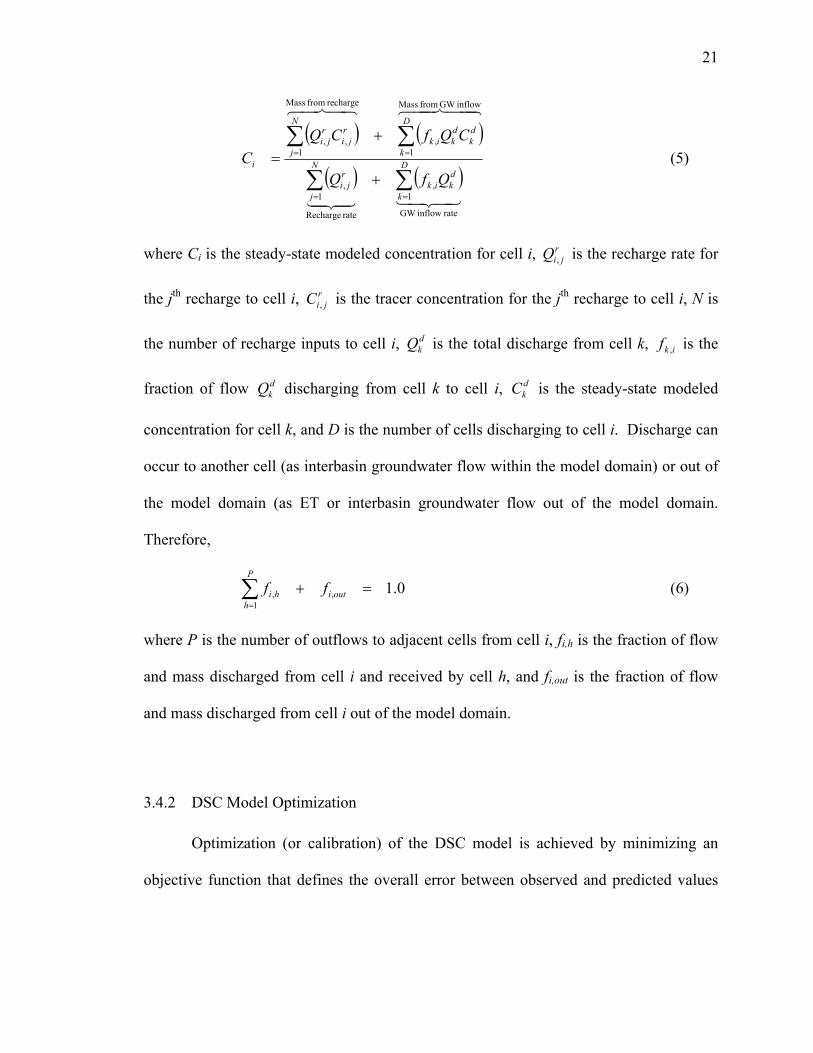
The steady-state assumption requires that volume and mass discharging from a

cell are equal to all inputs of volume and mass to that cell. The algorithm of an

instantaneously mixed cell may be expressed as:

21

( ) ( )

( ) ( )4342143421

448447648476

rate inflowGW

1,

rate Recharge

1,

inflowGW from Mass

1,

recharge from Mass

1,,

∑∑

∑∑

==

==

+

+= D

k

dkik

N

j

rji

D

k

dk

dkik

N

j

rji

rji

i

QfQ

CQfCQC (5)

where Ci is the steady-state modeled concentration for cell i, rjiQ , is the recharge rate for

the jth recharge to cell i, rjiC , is the tracer concentration for the jth recharge to cell i, N is

the number of recharge inputs to cell i, dkQ is the total discharge from cell k, ikf , is the

fraction of flow dkQ discharging from cell k to cell i, d

kC is the steady-state modeled

concentration for cell k, and D is the number of cells discharging to cell i. Discharge can

occur to another cell (as interbasin groundwater flow within the model domain) or out of

the model domain (as ET or interbasin groundwater flow out of the model domain.

Therefore,

0.1,1

, =+∑=

outi

P

hhi ff (6)

where P is the number of outflows to adjacent cells from cell i, fi,h is the fraction of flow

and mass discharged from cell i and received by cell h, and fi,out is the fraction of flow

and mass discharged from cell i out of the model domain.

3.4.2 DSC Model Optimization

Optimization (or calibration) of the DSC model is achieved by minimizing an

objective function that defines the overall error between observed and predicted values

22

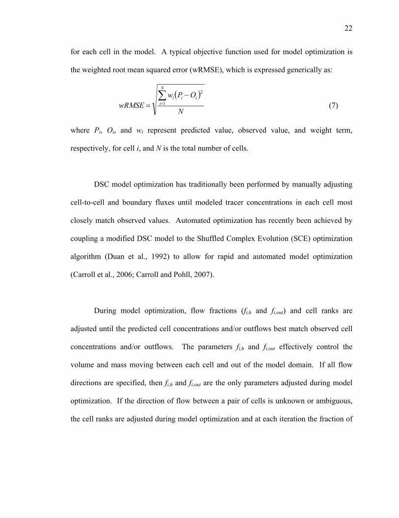
for each cell in the model. A typical objective function used for model optimization is

the weighted root mean squared error (wRMSE), which is expressed generically as:

( )

N

OPwwRMSE

N

iiii∑

=

−= 1

2

(7)

where Pi, Oi, and wi represent predicted value, observed value, and weight term,

respectively, for cell i, and N is the total number of cells.

DSC model optimization has traditionally been performed by manually adjusting

cell-to-cell and boundary fluxes until modeled tracer concentrations in each cell most

closely match observed values. Automated optimization has recently been achieved by

coupling a modified DSC model to the Shuffled Complex Evolution (SCE) optimization

algorithm (Duan et al., 1992) to allow for rapid and automated model optimization

(Carroll et al., 2006; Carroll and Pohll, 2007).

During model optimization, flow fractions (fi,h and fi,out) and cell ranks are

adjusted until the predicted cell concentrations and/or outflows best match observed cell

concentrations and/or outflows. The parameters fi,h and fi,out effectively control the

volume and mass moving between each cell and out of the model domain. If all flow

directions are specified, then fi,h and fi,out are the only parameters adjusted during model

optimization. If the direction of flow between a pair of cells is unknown or ambiguous,

the cell ranks are adjusted during model optimization and at each iteration the fraction of

23

flow from the lower (ranked) cell to the higher (ranked) cell is automatically set to zero

(Carroll et al. 2006).

3.5 Deuterium as a Groundwater Tracer

Deuterium (2H or D) and protium (1H) are the stable isotopes of hydrogen. The

isotope 1H is much more abundant than deuterium; on average the earth’s water supply

contains about one atom of D per 6,700 atoms of 1H, or about 0.015 percent D (Drever,

1997). The ratio of deuterium to protium (1H) is conventionally referenced to the Vienna

Standard Mean Ocean Water (VSMOW) standard by the equation:

1000

1

2

1

2

1

2

×

⎟⎟⎠

⎞⎜⎜⎝

⎛

⎟⎟⎠

⎞⎜⎜⎝

⎛−⎟⎟

⎠

⎞⎜⎜⎝

⎛

=

VSMOW

VSMOWsample

HH

HH

HH

Dδ (8)

where δD is the ratio, expressed as per mil (‰),of the difference between the D/1H ratios

of the sample and the reference to the D/1H ratio of the reference. Analytical error for δD

analyses is approximately 1 ‰ (Friedman et al., 2002).

Deuterium is a nearly ideal tracer for groundwater investigations because 1) it is

part of the water molecule and is therefore generally not affected by reactions with

geologic materials, and 2) it displays natural variability as a result of the processes of

evaporation and precipitation of water (Sadler, 1990). Deuterium data are useful for the

delineation of groundwater flow systems which include water from different source areas

(Thomas et al., 1996). The isotopic signature or characteristic for recharge water, basin-

fill aquifer groundwater, and deep carbonate-rock aquifer groundwater for various

24

groundwater flow systems within the Great Basin have been evaluated and used as a basis

for mixing models to calculate interbasin flow (Feeney et al., 1987; Roth and Campana,

1989; Kirk and Campana, 1990; Sadler, 1990; Thomas et al., 2001; Earman and Hershey,

2005; Carroll et al., 2006).

Freshwater systems are typically depleted in deuterium compared to oceanic

waters and consequently have negative δD values. The process by which water becomes

enriched in heavier isotopes (isotopically heavier, more positive δD values) or depleted in

heavy isotopes (isotopically lighter, more negative δD values) is referred to as

fractionation. Isotopic fractionation of water molecules occurs through a variety of

processes. When water evaporates, the resultant water vapor will be isotopically lighter

than the liquid water; when water vapor condenses as precipitation, the resultant liquid

water is isotopically heavier than the vapor (Drever, 1997). Variability in isotopic

composition of precipitation has been attributed to multiple effects, as summarized by

Hershey and Mizell (1995):

• temperature effect – fractionation during the formation of precipitation from

clouds is controlled by the temperature at which changes in physical state occur

• continental effect – precipitation tends toward more negative δ values further

away from the ocean

• altitude effect – precipitation becomes lighter (more negative δ values) at higher

altitudes

25

• latitude effect – precipitation becomes lighter (more negative δ values) at higher

latitudes

• amount effect – the greater the amount of precipitation, the more negative the δ

values

In addition, storm-to-storm variation in δD occurs, but mixing during the recharge

process causes smoothing toward the mean value (Gat, 1981; Darling and Bath, 1988).

Because evaporation changes δD values, any study using deuterium as a conservative

tracer should only examine a deep groundwater system that is minimally impacted by

evaporative processes. The characteristic δD value for recharge is defined with

groundwater springs in recharge source areas, as opposed to using precipitation δD values

that are highly variable and could be significantly altered by pre-recharge evaporation.

Groundwater springs in recharge areas represent surface expressions of precipitation

which has recharged, and may be assumed to average out storm-to-storm, seasonal,

yearly, and small geographic variations in the isotopic composition of precipitation

(Ingraham and Taylor, 1991). Assuming the effects of past climate regimes on deuterium

signatures are negligible and that alteration of the signature does not occur through

processes such as evaporation, then δD is simply a function of geographic location and is

therefore treated as a conservative tracer (Sadler, 1990).

The mass balance equation developed previously express mass flux as the product

of a tracer’s concentration (mass per volume) and a volumetric flow rate. A δD value is

26

not technically a concentration because it represents a difference between a water sample

and VSMOW rather than an amount of D per volume or mass of water. However, δD can

be treated as a concentration because it scales linearly with concentration and thus will

not cause a difference in mass balance model results versus use of an actual D

concentration.

4. METHODOLOGY

4.1 Approach

A groundwater accounting model was developed to evaluate basin and regional

water budgets for the BARCAS study area and to estimate rates of interbasin

groundwater flow within the study area and groundwater discharge to outside the study

area. Model and water budget uncertainties were evaluated via deterministic-sensitivity

and stochastic (Monte Carlo) uncertainty analyses.

The DSC model developed and applied for BARCAS is a single-layer model of

regional and deep intermediate groundwater within consolidated carbonate rock and

alluvium (Figure 3). For the context of the model, regional groundwater is defined as

having long flowpaths spanning multiple hydrographic areas, discharge far from

recharge, long travel times, and deep circulation. Deep-intermediate groundwater is

considered to be groundwater that does not traverse multiple basins; however, this water

does flow to sufficient depths to allow for heating and/or mixing with regional-type

groundwater. Both regional groundwater and deep-intermediate groundwater are

27

important to the study because these are the groundwater types that may be representative

of the regional aquifer.

Local groundwater systems, including shallow alluvial groundwater and perched

aquifers within mountain blocks, were not included as cells in the DSC model. Local

groundwater systems were not included as DSC model cells due to an insufficient amount

of data to support the increased optimization parameters associated with a multi-layer

model. However, groundwater samples collected from local systems were used to

estimate characteristic recharge δD values.

The DSC model was developed through a series of tasks related to geochemistry,

hydrology, modeling, and interpretation of results. The modeling approach included ten

tasks:

1. Compile deuterium database

2. Classify deuterium data as recharge, regional/deep-intermediate groundwater, or

neither

3. Identify model cells based on deuterium data and locations of intrabasin bedrock

highs

4. Calculate recharge deuterium values and rates for model cells

5. Calculate observed deuterium values for model cells

6. Identify possible interbasin flow occurrences and directions (cell connectivity)

7. Run deterministic groundwater accounting model

28

8. Estimate probability distributions for recharge rates, recharge deuterium values,

and groundwater ET discharge rates

9. Run Monte Carlo uncertainty analysis for groundwater accounting model

10. Present and discuss results

4.2 Assumptions

The following assumptions were made for the groundwater accounting model

(modified from Sadler [1990]):

1. The system is at steady-state.

2. Deuterium behaves as a conservative tracer in the mass-balance mixing model.

Fractionation of deuterium within the aquifer is assumed to not occur as a result

of residence time or flow within the aquifer, water-rock interactions, or ET

discharge.

3. The regional aquifer system may be represented as a series of cells, each of which

contains a characteristic deuterium concentration for the fully mixed cell

(sufficient data do not exist to subdivide into smaller cells).

4. The δD values used for calibration are representative of the δD content of

regional/deep-intermediate groundwater in the study area.

5. The δD values for recharge to the regional/deep-intermediate aquifer is related to

the δD values for springs, shallow wells, and some surface water within recharge

areas and downgradient of recharge areas.

29

6. Recharge rates and δD values have remained constant for a sufficient period of

time for steady-state conditions to be observed for the system. This assumption

does not imply that short-term fluctuations in recharge rates or values do not

occur; however, these fluctuations are assumed to be smoothed out (integrated)

over time to yield the estimated average value.

7. Groundwater input to the study area does not occur as interbasin groundwater

flow from outside the study area. This assumption implies that the only

groundwater input to the system occurs as recharge from precipitation. Water

budgets presented in previous reports identified “some” groundwater inflow to

Little Smoky Valley from Stevens Basin and Antelope Valley (Rush and Everett,

1966) and unspecified amounts of groundwater inflow to Snake Valley from Pine

Valley and Wah Wah Valley (Harrill et al., 1988). Groundwater inflow from

outside the study area to Little Smoky Valley and Snake Valley was not modeled

due to the non-quantitative nature of estimates for inflow reported in previous

studies.

4.3 Deuterium Database

Deuterium data were used to assign characteristic recharge and mixed cell δD

values and as a criterion for subdividing the larger basins of the study area into sub-

basins. Deuterium data were managed in a database of stable isotope (deuterium,

oxygen-18) sample results compiled for the study area and adjacent basins. Associated

chemical parameters (e.g. temperature, specific conductance, chloride, sulfate, tritium,

30

etc.) were also included in the database for use in classifying sample locations. The

database was queried from the USGS National Water Information System (NWIS)

database (Reference). The NWIS database was updated during the BARCAS study to

include relevant historic USGS samples, samples from previous DRI reports, unpublished

theses, and samples collected for the BARCAS geochemistry task.

Plots of deuterium versus oxygen-18 were prepared to identify samples which are

evaporated relative to global and local meteoric water lines. Sample locations with

deuterium data were classified as 1) representative of recharge, 2) representative of

regional/deep-intermediate type groundwater, or 3) neither representative of recharge or

regional/deep-intermediate type groundwater. Sample classification was based on

primarily on the location and water temperature; however, additional criteria were also

used:

• previous studies which identified springs and wells as representative of

regional groundwater (Harrill et al. 1988, Beddinger et al. 1985)

• revised regional potentiometric surface map for the BARCAS study area

• interpreted dissolved gas data (Hershey et al. 2007)

• surrounding geology

• conventional chemical parameters, such as sodium-potassium-sulfate-

chloride plots described by Mifflin (1968)

Two-hundred thirty nine sample sites were identified as representative of recharge

or potential recharge; these sites are listed in Appendix A and are shown on Figure 6.

31

Samples collected from springs, shallow groundwater wells, and some surface water sites

were identified as representative of recharge or potential recharge based on one or more

of the following criteria: cool water temperature, topographic setting, location relative to

recharge areas, discharge characteristics (springs), surrounding geology, well depth,

elevation relative to regional potentiometric surface, and variability in discharge rate or

chemistry.

A total of 84 sites were identified as representative of regional / deep-intermediate

groundwater; these sites are shown on Figure 7 and listed in Appendix B. Waters

representative of regional or deep-intermediate groundwater were identified based on

warm water temperatures, surrounding geology, depth of the regional potentiometric

surface, deuterium composition relative to nearby recharge, previous reports identifying

regional and large springs of the Basin and Range province (Bedinger et al., 1985; Harrill

et al., 1988), and results from a geochemical evaluation of dissolved gases within

groundwater samples collected for the BARCAS study (Hershey et al., 2007). Regional

or deep-intermediate groundwater samples generally had temperatures greater than about

68 degreed Fahrenheit. In some cases, plots of conventional chemical parameters, such

as sodium-potassium-sulfate-chloride plots described by Mifflin (1968) were used to

provide additional support for sample classifications.

32

4.4 Model Inputs

The following subsections describe the specific assumptions and input parameters

associated with the BARCAS DSC model, which serves as the “base case” for model

evaluation. Revised assumptions and input parameters associated with the uncertainty

analysis are provided in Section 4.6.

4.4.1 Model Cells

Model cells were identified based on hydrographic area boundaries and locations

of intrabasin bedrock highs. Deuterium data for regional/deep-intermediate groundwater

was compared with the locations intrabasin bedrock highs within the BARCAS study

area (Welch and Bright, in review) to determine which basins support division into sub-

basins. Intrabasin bedrock highs and DSC model cells are shown on Figure 8.

4.4.2 Cell Connectivity

The potential groundwater flowpaths between model cells shown on Figure 8

were identified based on the hydrographic area boundary classifications determined for

the geology task and the regional potentiometric surface contours (Welch and Bright, in

review). Boundary classifications for probable flow (green) or possible flow (yellow)

were compared to the potentiometric surface in adjacent basins. If a gradient was present,

then a potential interbasin flow was identified. If interbasin flow was possible based on

the hydrographic boundary classification, but a gradient between basins was not apparent

33

based on the regional potentiometric surface, then a potential interbasin flow was

identified with an undetermined direction. If a basin boundary was classified as flow not

likely (red) or if a groundwater mound was present, no potential flow was identified.

Potential interbasin groundwater flows were used to establish the cell network for the

DSC model and are shown in Figure 8.

Interbasin groundwater flows out of the model domain are not shown on Figure 8

nor are these flows explicitly listed in the model’s input or output. The DSC model

predicts one rate for output from the model domain for each cell, and this rate of output

from the model domain is not divided into components of interbasin groundwater flow

and discharge as groundwater ET. Groundwater flow out of the model domain (or study

area) may be estimated, however, by subtracting an estimated groundwater ET discharge

rate from the total output from the model domain.

4.4.3 Head Rankings

Model cells were assigned head rankings from 1 (lowest head) to 20 (highest

head) based on the regional potentiometric surface map generated under the BARCAS

groundwater flow task (Welch and Bright, in review). Head rankings were assigned by

calculating the average regional aquifer potentiometric elevation in each cell. Average

elevations were determined by performing a simple interpolation of contour lines to

generate a continuous potentiometric surface, then calculating the average value using

ARCMap 9 geographic information system (GIS) software. Average heads ranged from

34

4,496 feet above mean sea level (amsl) for the northeast portion of Snake Valley to 6,747

feet amsl for the southern portion of Steptoe Valley. Average heads and head rankings

are listed in Table 5 and shown on Figure 8.

4.4.4 Recharge Rates

Recharge rates for each cell were determined from the recharge estimates

calculated for the BARCAS recharge task using the basin characterization model (BCM)

methodology (Welch and Bright, in review). Summations of potential in-place recharge

and potential runoff were calculated from the 886-foot grid BCM output using

geographic information system (GIS) software. The assumed ratio of 15 percent of

potential runoff becoming recharge was maintained for cell recharge estimates for

consistency with the BARCAS recharge task. Calculations also assumed that topographic

basin boundaries were representative of hydrographic area boundaries. Recharge rates in

acre-feet/year for each cell are presented on Table 5.

4.4.5 Recharge δD Values

Recharge δD values were determined based on the identified recharge samples

and the spatial distribution of recharge across the study area. Recharge δD data are not

available for all areas where recharge is predicted to occur. To determine δD values in

areas without data and to calculate deuterium values at unsampled locations, the recharge

data set was interpolated using an inverse distance weighting (IDW) algorithm. The

interpolated recharge δD prediction map, shown in Figure 6, was generated using GIS

35

and provides δD values for recharge at a 886-foot grid scale. The prediction map shows a

pronounced trend in recharge δD values from isotopically heavier recharge δD in the

south (warmer colors) to isotopically lighter recharge δD in the north (cooler colors) and

suggests that at the scale of the study area, deuterium content is most influenced by

latitude. The extent of the prediction map was limited to the east and west by the

available recharge data. As such, the prediction map does not cover recharge areas in

eastern Little Smoky Valley and the western portion of Snake Valley. These areas

contribute relatively little recharge to the respective basins.

The final step in determining the δD value for recharge was to calculate a

recharge-weighted average for each basin or sub-basin in the study area. Recharge-

weighted average δD values were determined by multiplying the total potential recharge

rate by the predicted recharge δD value for each 886-foot grid cell, summing these for the

entire (sub)basin, then dividing by the total recharge rate for the entire (sub)basin. The

resulting recharge-weighted averages are shown in Figure 6 and listed in Table 5.

Recharge-weighted averages for Little Smoky Valley and select sub-basins of Snake

Valley were estimated based on the extent of the interpolated recharge prediction map.

36

4.5 Calibration Parameters

4.5.1 Observed δD Values

Observed δD values were determined from the deuterium database. Regional /

deep-intermediate groundwater sample locations are shown in Figure 7. Observed δD

values for each cell were calculated as the average of all δD values for applicable sites

within or in some cases near a model cell. No appropriate δD data were identified for

Butte Valley, Jakes Valley, and the central portion of Snake Valley; therefore, observed

δD values were not calculable for the cells corresponding to these basins. Observed δD

values for DSC model cells are shown on Figure 7 and listed in Table 5.

4.5.2 Observation Weights

During model optimization, the errors between observed and predicted δD values

for each cell were incorporated into an overall objective function using weighting criteria.

The weighting criteria account for differing uncertainty in observed δD values and for

most model cells were calculated as:

⎟⎟⎠

⎞⎜⎜⎝

⎛

−

=

− 1

1

1,05.0i

in

c

ns

t

w

i

i (9)

where icw is the observed δD value weight for cell i, n is the number of regional / deep-

intermediate-type groundwater samples associated with cell i, si is the standard deviation

of observed values, and t is the Student t-statistic with α = 0.10 and df = ni-1. The

37

denominator for this weight function is analogous to one-half the 90-percent confidence

interval about the observed mean, giving the δD weight units of ‰-1.

This weight function effectively takes into account both the number and the

variability of data points used for calculating the observed concentration values (Carroll

and Pohll, in press) and assumes that the variance in the observed concentration for a

given cell is independent from observed variance in other cells’ concentrations. This

approach is consistent with the approach described by Hill (1998), who suggests that

weights should be proportional to the inverse of the variance-covariance matrix. The

inverse variance gives greater weight to more accurately observed values and lower

weight to less accurately observed values. The inverse variance also effectively

normalizes observed values such that one can use different parameters in the objective

function.

Observed δD value weights for DSC model cells are presented in Table 5.

Observed value δD weights were calculated as described above with the following

exceptions:

• Butte Valley, Jakes Valley, and the central portion of Snake Valley had no

observed δD values; therefore, the weights for these cells were set to zero.

• Calculation of standard deviation and confidence interval for observed δD

values was not possible for Newark Valley and the northern portion of

38

Spring Valley because only one regional / deep-intermediate-type

groundwater δD sample was identified for each of these cells (n = 1

sample). Observed δD value weights for these cells were assumed to be

0.1 ‰-1 to reflect relatively low confidence in the associated observed δD

values.

• Calculation of the inverse confidence interval was not possible for the

northeastern portion of Snake Valley due to a zero standard deviation for

the observed δD values for this cell (n = 2 samples). The observed δD

value weights for the northeastern portion of Snake Valley was assumed to

be 0.5 ‰-1 to reflect an intermediate confidence in the associated

observed δD value.

• The calculated inverse confidence interval for Long Valley (0.04 ‰-1) was

about two orders of magnitude less than inverse confidence intervals

calculated for other cells. The observed δD value weight for Long Valley

was assumed to be 0.1 ‰-1 in order to reflect low confidence the observed

δD value while keeping the error contribution from this cell to the overall

objective function within the same order of magnitude as other cells in the

model.

39

4.5.3 Groundwater ET Discharge Weights

For some model runs, optimization included a comparison of groundwater

outflow from each cell to the groundwater ET rates calculated under the BARCAS

Discharge Task (Welch and Bright, in review). In these cases, the BARCAS groundwater

ET rates represent hypothetical minima for outflow rates from cells in the model.

Standard deviations associated with the groundwater ET estimates for each basin and

sub-basin were also calculated under the Discharge Task (Zhu, in press). Groundwater

ET rates and their associated standard deviations are shown in Table 5.

For cell outflows, weights were calculated as the inverse of the standard deviation

of the groundwater ET rate ( GWETs ):

GWETQ s

wi

1= (10)

where iQw is the groundwater ET rate weight with units of (acre-feet/year)-1.

4.5.4 Objective Functions

Weighted root mean squared error (wRMSE) or variations thereof were used as

objective functions for model optimization. Early in the modeling process it became

apparent that when optimized based only δD values, model-predicted rates for

groundwater discharge from the model domain for multiple basins differed significantly

from estimated groundwater evapotranspiration rates. To target δD values and discharge

40

rates, the model was run using three optimization scenarios: c, o, and o*. Scenario c

optimized the model based on target concentrations (δD values) only. Scenarios o and o*

both optimized the model based on target δD values and groundwater ET rates. Scenario

o penalized the model if a basin’s discharge out of the model domain was less than the

groundwater ET rate, while scenario o* incorporated more rigorous constraints on

discharge rates for cells in the interior of the model domain. The weight terms for both

concentration and outflow are squared when used in the objective function(s) to become

the dimensionally correct inverse variance term suggested by Hill (1998).

Each optimization scenario had a specific objective function. The optimization

scenarios and associated objective functions are described below.

Optimization Scenario C

Under scenario C, the model was optimized based on concentration only. This

approach is consistent with traditional applications of the DSC model. The objective

function for scenario c is expressed as:

( )5.0

1

22

⎟⎟⎟⎟

⎠

⎞

⎜⎜⎜⎜

⎝

⎛−

=∑=

N

CpCowwRMSE

N

iiiic

c (11)

41

where Coi and Cpi are the observed and predicted concentrations in cell i, respectively, N

is the number of cells being modeled, and iwc is the weight assigned to cell i for the

observed concentration.

Optimization Scenario O

Model optimization scenario O included both concentration and outflow in the

objective function. Scenario O penalized the model if a basin’s discharge out of the

model domain was less than the groundwater ET rate. The objective function for scenario

o is modified as follows:

( ) ( )5.0

1 1

2222

2 if; 0

if;

⎟⎟⎟⎟⎟

⎠

⎞

⎜⎜⎜⎜⎜

⎝

⎛

⎭⎬⎫

⎩⎨⎧

≥<−

+−

=∑ ∑= =

NQQ

QQQQwCpCowwRMSE

N

i

N

i ETout

EToutioutiETiQiiic

o (12)

where iETQ and ioutQ are the groundwater ET rate from the BARCASS discharge task

and the cell outflow predicted by the DSC model, respectively, and iQw is the weight

assigned to the groundwater ET rate.

Optimization Scenario O*

Given the extent of the study area, the assumed DSC model cell connectivity,

and/or the interpreted hydrogeologic boundaries, groundwater outflow out of the model

domain is not possible for cells 4 (southern Spring Valley), 7 (northern White River

42

Valley), 9 (southern Steptoe Valley), 10 (Jakes Valley), 11 (central Steptoe Valley), 15

(central Spring Valley), and 16 (northern Spring Valley) (Figure 8). For example,

northern White River Valley is surrounded by other DSC model cells to the north, east

and south and by a geologic structure to the west through which groundwater flow is not

likely. For these cells, groundwater outflow from the model should only consist of

groundwater ET. In order to deter excessive predicted outflow rates for these cells, the

objective function was modified for scenario O*.

Model optimization scenario O* included both concentration and outflow in the

objective function. Scenario O* incorporated more rigorous constraints on discharge rates

for interior cells by penalizing the model for any difference between discharge out of the

model domain and target groundwater ET rates for the interior cells of the model domain.

Under this scenario, the objective function is expressed as:

( )( )

( )

5.0

1 1 22

22

22

2

int, if if0 if

⎟⎟⎟⎟⎟⎟⎟⎟⎟

⎠

⎞

⎜⎜⎜⎜⎜⎜⎜⎜⎜

⎝

⎛

⎪⎭

⎪⎬

⎫

⎪⎩

⎪⎨

⎧

≠−≥<−

+−

=

∑ ∑= =

N

QQQQwQQQQQQw

CpCow

wRMSE

N

i

N

iEToutioutiETiQ

ETout

EToutioutiETiQ

iiic

o(13)

where different criteria apply to interior (int) model cells.

43

4.6 Uncertainty Analysis

Having developed the base DSC model for the BARCAS study area, in Sections

4.4 and 4.5, the next step was to evaluate model uncertainty. The uncertainty analyses

may be generally classified as either deterministic-sensitivity or stochastic types.

Deterministic-sensitivity type analyses were performed by varying either a single set of

model inputs (e.g. average recharge δD values for cells) or the objective function and

evaluating the effect on model output. This type of analysis generates one set of model

output for each variation, and is therefore used to evaluate the sensitivity of deterministic

model results. Stochastic type uncertainty analyses were performed by running Monte

Carlo simulations with the model, where model parameters are assigned distributions of

values (rather than single values) and the model is run repeatedly using randomly-

selected values for model parameters. Output from stochastic type uncertainty analyses

includes many sets of model output.

The following sections describe the deterministic-sensitivity and stochastic

uncertainty analysis which were performed.

4.6.1 Deterministic-Sensitivity Uncertainty Analyses

Deterministic-sensitivity type analyses were performed by varying either a single

set of model inputs or the objective function. The analyses incorporated different

recharge δD value estimation methods and/or the selected objective function for model

optimization. A total of seven deterministic-sensitivity analyses were performed by

44

combining four optimization approaches and two recharge δD value estimation methods.

The salient characteristics for the seven deterministic-sensitivity analyses (numbered DS-

1 through DS-7) are presented on Table 6. Analyses DS-1, DS-2, and DS-3 represent the

base BARCAS DSC model, where recharge δD value estimation and model optimization

were performed as described in Sections 4.4.4 and 4.5.4, respectively. Analyses DS-4,

DS-5, and DS-6 maintain the base BARCAS optimization scenarios, but use an

alternative method for estimating recharge δD values, described below. Analysis DS-7

uses recharge δD values from the base BARCAS model, but uses a new objective

function for model optimization.

Recharge δD Value Estimation Methods

Two recharge δD estimation methods were used for the deterministic-sensitivity

analyses. The first is the method used for the base BARCAS DSC model, described in

Section 4.4.5, where representative recharge δD values for model cells were determined

from a prediction map for recharge deuterium δD values developed using an inverse

distance weighting (IDW) interpolation algorithm. The IDW algorithm generates a

continuous prediction map over the horizontal and vertical extent of the data set;

however, the BCM model predicts no recharge to occur at the valley floors of the study

area basins. The distribution of BCM-predicted recharge is shown on Figure 6, where the

IDW-interpolated recharge δD values have been masked in areas where zero recharge is

predicted by the BCM model. The distribution of recharge, including areas with zero

45

predicted recharge, was factored into the calculated recharge δD values by using

recharge-weighted averages for recharge δD values for model cells.

A second, simpler method for estimating recharge δD values was developed using

a simple linear regression of recharge sample δD values against latitude. Figure 9 is a

plot showing average δD values for recharge samples versus latitude. Regressing average

δD values against latitude yields the relationship:

44.40014.13 +×−= LattitudeDRδ (14)

where δDR is the predicted recharge δD value and Latitude is in decimal degrees, North

American Datum 1983 (NAD1983). The coefficient of determination (r2) for the

regression is 0.78, indicating that variability in recharge δD value is explained reasonably

well by latitude. Recharge δD values for model cells were calculated by applying the

latitude regression equation to the latitude for each model cell’s centroid. Model cell

centroids were determined using GIS. Recharge δD values for model cells estimated by

the IDW-interpolation and latitude regression methods are shown in Table 7.

Objective Functions

A total of four objective functions were used for the deterministic-sensitivity

uncertainty analysis. The first three objective functions correspond the optimization

scenarios c, o, and o* for the base BARCAS DSC model, described in Section 4.5.4.

Optimization scenarios c, o, and o* incorporated target δD values and discharge rates to

varying degrees using a weighted root mean squared error (wRMSE) type objective

46

function (see equations 11, 12, and 13). The fourth objective function is the sum of

absolute errors for concentrations (SAEC), which is expressed as:

∑=

−=oN

iiiC CpCoSAE

1 (15)

where Coi and Cpi are the observed and predicted concentrations (δD values),

respectively, for cell i and No is the number of cells with observed concentrations. The

SAEC function provides a non-weighted objective function which reduces the potential

overweighting of large errors that may occur with squared error type functions such as

root mean squared error (RMSE). As only concentration is used for model optimization,

the SAEC function is similar to the wRMSEC function used for optimization scenario c of

the base BARCAS DSC model. Incorporating both target discharge rates and δD values

into a non-weighted objective function is unattractive due to the different physical

dimensions of discharge rates and δD values.

4.6.2 Monte Carlo Uncertainty Analyses

Stochastic uncertainty analyses were performed by running a series of Monte

Carlo simulations. The Monte Carlo uncertainty analysis was performed by randomly

sampling model parameters from distributions for a given realization, then running the

model to achieve the best fit for that realization. The process is then repeated with new

random values selected for model parameters. A total of 1,000 realizations were

performed in this fashion.

47

The Monte Carlo simulations included a variety of distributions for cell recharge

rates, recharge δD values, and target discharge rates. Seven Monte Carlo simulations

were developed by combining three distributions for recharge rates and δD values, two

distributions for target groundwater discharge rates, and three optimization approaches.

To evaluate the uniqueness of model results, an eighth Monte Carlo simulation was

performed by running 1,000 simulations of a model using constant values for model

parameters. The salient characteristics of the eight Monte Carlo simulations, referred to

as MC-1 through MC-8, are presented on Table 8. The following subsections describe

the distributions for recharge rate, recharge δD values, and target groundwater discharge

rates.

Recharge Rates

Monte Carlo simulations MC-1 through MC-7 included one of three distributions

for recharge rates. Recharge rate distributions were identified 1) from BCM-predicted

recharge rates and associated uncertainty described for the BARCAS study, 2) using the

bootstrap brute force recharge model (BBRM) developed by Epstein (2004) to calculate

recharge distributions, and 3) through an evaluation of ranges of recharge rates presented

in the BARCAS study and previous studies. For simulation MC-8, recharge rates were

kept constant using BARCAS BCM-predicted rates where 15 percent of runoff was

assumed to become recharge.

48

As described in Section 4.4.4, recharge rates calculated for the BARCAS study by

the BCM methodology assumed that total recharge equals potential in-place recharge

plus 15 percent of potential runoff. The uncertainty associated with recharge predictions

by the BCM method is greater for areas with a larger component of potential runoff (Flint

and Welch, in review). A range of BCM-predicted recharge rates was evaluated by

adjusting the proportion of potential runoff becoming recharge between 0 percent and 30

percent while keeping the amount of potential in-place recharge constant. Recharge

calculations were performed using GIS and the coverages for potential in place recharge

and potential runoff from the BCM. A uniform distribution of recharge rates was then

generated using this range of BCM-predicted recharge rates for Monte Carlo simulations

MC-1, MC-2, and MC-3. Ranges of BCM-predicted recharge rates for model cells are

shown on Figure 10.

Distributions for recharge rates were also developed by applying the BBRM. The

BBRM method relates recharge to precipitation using four precipitation intervals from

the PRISM map and multiplying the annual amount of precipitation by a coefficient

relating volume recharged to precipitation volume (Epstein 2004). BBRM coefficients

were determined by a bootstrap selection for 1,000 realizations, with each realization

using one million brute-force inverse optimization iterations. By using the coefficients

from each of the 1,000 realization, a distribution of recharge rates was developed for each

model cell. The PRISM map showing precipitation intervals for the study area is

provided in Figure 11. Precipitation volumes associated with each precipitation interval

for each model cell were calculated using GIS by multiplying the area of each

49

precipitation interval by the precipitation amount. Precipitation volumes were summed

for the precipitation intervals used in the BBRM (0 to 10 inches, >10 to 20 inches, >20 to

30 inches, and >30 inches) and recharge volumes were then calculated by multiplying

precipitation volumes for each interval by the appropriate coefficient. The precipitation

volumes for each interval did not change between realizations; only the recharge

coefficients. The BBRM method generated 1,000 recharge rates for each model cell

which were input directly into the DSC model for use in Monte Carlo simulations MC-4

and MC-5. The upper and lower bounds of the 95% confidence interval for each basin’s

BBRM recharge are shown on Figure 10. The confidence interval was calculated by

sorting the recharge rates for each cell then taking the 26th and 975th value from the sorted

rates. The confidence intervals shown on Figure 10 reflect the total recharge to each

basin; therefore, the recharge volumes for associated sub-basins were totaled for those

basins which are divided into sub-basins (Snake Valley, Spring Valley, Steptoe Valley,

and White River Valley).

The third method used for developing recharge rate distributions was based on the

ranges of recharge rates provided in previous studies and from the BARCAS study. As

described in Section 3.3.2, a variety of previous studies have included recharge estimates

for hydrographic area in the BARCAS study area. The individual values from previous

studies are presented on Table 1 and the ranges of estimates are shown on Figure 10. The

distributions for recharge for Monte Carlo simulations MC-6 and MC-7 were identified

based on the minimum and maximum estimates from previous studies, the BARCAS

BCM-predicted rates, and the rates calculated using the BBRM, described above. These

50

minimum and maximum rates defined the lower and upper bounds for a uniform

distribution of recharge rates. Because previous studies have not used the same basin

subdivisions as were used for the DSC model cells, the net recharge for the entire basin

(i.e. the sum of individual sub-basins) was compared to recharge estimates from previous

studies for hydrographic areas which were subdivided for the DSC model (Figure 10).

For White River Valley, the maximum recharge rate was reported by Thomas et al.

(2001). In order to estimate maximum values for recharge rates associated with the

White River Valley sub-basins, the maximum rates from the BBRM model were

multiplied by a factor equal to the maximum BBRM recharge for White River Valley

divided by the White River Valley recharge reported by Thomas et al. (2001). This

approach facilitated estimates for maximum recharge rates which summed to the

maximum value while keeping the same proportion of recharge associated with each sub-

basin. A similar method was used for generating sub-basin minimum recharge rates for

Snake Valley, Spring Valley, and Steptoe Valley, where the minimum reported recharge

rates are by Flint et al. ([2004], Snake Valley) and by Watson et al. ([1976], Spring

Valley and Steptoe Valley). Ranges for recharge rates calculated for the minimum and

maximum of available estimates are shown on Figure 10.

Recharge δD Values

Three distributions for recharge δD values were developed for Monte Carlo

simulations MC-1 to MC-7. Uniform distributions were assumed for recharge rates and

51

δD values based on insufficient data to support the selection of more specific

distributions. Monte Carlo simulation MC-8 used constant recharge δD values.

The recharge δD distributions for simulations MC-1 to MC-5 were created by

varying model cells’ recharge δD values by a factor of ± 1.5 ‰. This factor was selected

based on the typical analytical variability of deuterium analyses (± 1 ‰) and the

variability of δD values for groups of samples from within zones of high recharge rates.

For simulations MC-1 to MC-3, model cells’ recharge values were calculated from the

BCM-predicted recharge distribution and IDW-interpolated recharge δD prediction map,

as described in Section 4.4.5. This method was consistent with the use of BCM recharge

rates for these Monte Carlo simulations. As simulations MC-4 and MC-5 used

distributions of model cell recharge rates created using BBRM, recharge δD values for

model cells were calculated based on the spatial distribution of recharge from the BBRM

and the IDW-interpolated recharge δD prediction map. This calculation was performed

using the mean coefficients from all BBRM bootstrap realizations. Recharge

distributions were then created by varying model cells’ recharge δD values by ± 1.5 ‰.

The third recharge δD distribution was developed to represent the potential range

of δD values which are calculable based on combinations of the ranges of recharge

distributions calculated by BCM and BBRM methods and the recharge δD prediction

maps interpolated using the IDW algorithm and latitude regression. Using GIS, spatial

recharge distributions were developed representing BCM-predicted recharge with

assumed potential runoff to recharge factors of 0 percent, 15 percent, and 30 percent.

52

Spatial recharge distributions were also developed for the recharge predicted by the

BBRM using the average coefficient values and the sets of coefficients which resulted in

the minimum and maximum recharge rates. Each of these six spatial recharge

distributions was then combined with the IDW and latitude regression recharge δD

prediction maps to yield twelve potential recharge δD values for each model cell (Table

9). An additional set of recharge δD values were developed by applying the latitude

regression model (see equation 14) to the centroid of each model cell. Centroids for

model cells were calculated using GIS. The regression model was also used to calculate

the upper and lower limits of the 95 percent confidence interval on the mean recharge δD

value for model cell centroids.

The twelve recharge δD values calculated by combining spatial recharge

distributions with δD prediction maps and the three recharge δD values calculated using

the latitude regression model (mean, lower 95 percent confidence limit, upper 95 percent

confidence limit) provided a total of fifteen basis values for determining minimum and

maximum recharge δD values for each model cell (Table 9). The minimum and

maximum basis δD values were used to define recharge δD value distribution if the

difference between minimum and maximum basis δD values was greater than or equal to

3 ‰. If the difference between minimum and maximum basis values was less than 3‰,

the recharge δD value distribution was assumed to equal the average of the minimum and

maximum basis values ± 1.5 ‰. Recharge δD distributions are provided on Table 10.

For comparison purposes, Table 10 also includes recharge δD values calculated as the

53

simple average of all recharge samples within 6.2 miles of a model cell, as well as

average recharge values presented in previous studies, where available.

Target Groundwater ET Discharge Rates and Weights

Target groundwater ET discharge rates were used for Monte Carlo simulations

where the DSC model included target discharge rates in its objective function. As shown

on Table 8, optimization scenario o was used for Monte Carlo simulations MC-2, MC-5,

MC-7, and MC-8 and optimization scenario o* was used for simulation MC-3. Target

groundwater ET rates were kept constant in simulations MC-2 and MC-3; therefore,

uncertainty associated groundwater ET rate estimates are not incorporated in these Monte

Carlo uncertainty analysis. This may limit the predicted uncertainty bounds for

interbasin flow estimates. Constant groundwater ET discharge rates were also used with

simulation MC-8, consistent with the constant values used for other model parameters in

this simulation. Distributions for target discharge rates for simulations MC-5 and MC-7

were identified based on results from an uncertainty analysis of estimated groundwater

ET rates performed for BARCAS study (Zhu 2006) and the ranges of groundwater ET

estimates available from previous and current studies, respectively.

Uncertainty analysis for groundwater ET discharge rates was completed for the

BARCAS study by performing a 10,000-realization Monte Carlo simulation for discharge

calculations using assumed distributions for each calculation parameter (ET unit rates,

unit areas, and precipitation) for each (sub)basin in the study area (Zhu 2006). The

54

resulting distributions of groundwater ET discharge rates resemble normal-type

distributions, i.e. the probability distribution functions are reasonably bell-shaped. The

standard deviations from the distributions of groundwater discharge provided the basis

for target discharge rate weighting criteria described in Section 4.5.3. For the DSC

model uncertainty analysis, 1,000 groundwater ET discharge rates were selected from the

10,000 realizations performed for the BARCAS groundwater ET discharge uncertainty

analysis. These 1,000 groundwater ET discharge rates were input directly into the DSC

model for use in Monte Carlo simulation MC-5. The upper and lower bounds of the 95%

confidence interval for groundwater ET discharge rates are shown in Figure 12. The

confidence interval was calculated by sorting the groundwater ET discharge rates for

each cell then taking the 26th and 975th value from the sorted rates.

A comparison between the sum of recharge rates for all model cells and the sum

of total target groundwater ET discharge for all model cells was made for each Monte

Carlo realization in simulation MC-5. If the total recharge for a realization was less than

the total target groundwater ET discharge, then that realization was skipped. This step

was necessary to be consistent with the assumption that groundwater input to the study

area does not occur as interbasin groundwater flow from outside the study area, and to

prevent the use of unrealistic model parameters when optimization included target

groundwater ET discharge rates. Of the 1,000 sets of recharge and groundwater ET

discharge rates identified for simulation MC-5, 260 sets had total recharge less than total

target groundwater ET discharge and were skipped, resulting in 740 Monte Carlo

realizations for simulation MC-5.

55

For Monte Carlo simulation MC-7, target groundwater ET distributions were

developed as uniform distributions using the minimum and maximum groundwater ET

rates presented in previous studies and from the BARCAS study. Groundwater ET

discharge rates from previous studies are described in Section 3.3.2 and presented in

Table 2. Figure 12 shows groundwater ET discharge rates from previous studies along

with the 95% confidence interval for groundwater ET discharge rates calculated for the

BARCAS groundwater ET discharge uncertainty analysis. For model cells representing

entire basins, the range for target groundwater ET rates was defined by the minimum and

maximum rates from previous studies and the BARCAS study as shown on Figure 12.

For model cells which represent sub-basins of Snake Valley, Spring Valley, Steptoe

Valley, and White River Valley a comparison was made between ranges of estimates of

groundwater ET discharge rates was made on a net-basin basis. As the 95% confidence

intervals for BARCAS study groundwater ET discharge rates encompassed the minimum

and maximum estimates from previous studies, the 95% confidence intervals for

BARCAS study groundwater ET discharge rates were used to define the upper and lower

limits of the groundwater ET discharge rate distributions for Snake Valley, Spring

Valley, and Steptoe Valley for Monte Carlo simulation MC-7. In White River Valley,

the groundwater ET discharge rate presented in Water Resources Bulletin 33 (Eakin

1966) was less than the lower limit of the 95 percent confidence interval for the

BARCAS study groundwater ET discharge estimate. In order to estimate minimum

values for groundwater ET discharge for the White River Valley sub-basins, the lower

limits from the 95% confidence intervals for BARCAS study groundwater ET discharge

56

rates for each sub-basin were multiplied by a factor equal to the lower limit for the

BARCAS 95% confidence interval for net groundwater ET discharge for White River

Valley divided by the White River Valley groundwater ET discharge reported by Eakin

(1966). This approach is consistent with the development of the recharge distributions

for simulations MC-6 and MC-7, described above.

As described above for simulation MC-5, a comparison between total recharge

and total groundwater ET discharge was also necessary for simulation MC-7. Whereas

for MC-5 a discrete set of 1,000 realizations were available for recharge and groundwater

ET discharge rates, an infinite number of recharge and groundwater ET discharge rates

for simulation MC-7 could be generated using the uniform distributions described above.

For each realization of Monte Carlo simulation MC-7, model-generated recharge rates

and groundwater discharge rates were summed for all cells and compared. If the total

recharge was less than the total groundwater ET discharge, that set of values was

discarded and a new set was generated. In this manner it was possible to run 1,000

realizations which met the requirement that total recharge was greater than total

groundwater ET discharge.

For each realization of Monte Carlo simulations MC-5 and MC-7, groundwater

ET discharge weights for each cell were calculated as the inverse of the product of the

coefficient of variation of the BARCAS study groundwater ET rate for cell i ( iGWETCV )

and the target groundwater ET discharge rate of cell i for realization n (niGWETQ

,):

57

ni

niGWETiGWET

GWET QCVw

,

,

1×

= (16)

where iQw is the groundwater ET rate weight for cell i with units of (acre-feet/year)-1.

This approach adjusted the weighting terms according to the magnitudes of the

groundwater ET discharge rates. Coefficients of variation for BARCAS study

groundwater ET rates were calculated by dividing the standard deviation of the

groundwater ET rate by the estimated BARCAS groundwater ET rate (Table 5).

5. MODEL RESULTS

This section is broken into three parts: results from deterministic modeling for the

base BARCAS DSC model, results from the deterministic-sensitivity uncertainty

analyses, and results from the stochastic (Monte Carlo) uncertainty analyses. For each

model run, the DSC model generated as output the set of volumetric groundwater flow

rates between model cells and out of the model domain that best satisfied the

optimization criteria. Model output also included predicted δD values and objective

function values.

5.1 BARCAS DSC Base Model

The results from the base BARCAS DSC model provide the first set of results as

a base case against which subsequent model results can be compared. The DSC water

budget accounting model was applied using recharge estimates and groundwater ET

58

discharge rates from the BARCAS study. The deterministic model results from one of

these model runs provided the interbasin and intrabasin groundwater flow rates reported

in the BARCAS SIR (Welch and Bright, in review). The BARCAS DSC model is

documented in the DRI satellite report which was prepared for the BARCAS study

(Lundmark et al., 2007). In addition to their relevance with respect to the BARCAS

study, the results from the base BARCAS DSC model provide examples for evaluating

the effects on model optimization approach, a topic examined in more detail in the

deterministic-sensitivity analysis section of this report.

Three sets of results were generated for the base BARCAS DSC model; one set

for each of the three optimization scenarios C, O, and O*. For each optimization

scenario, the DSC model generated as output the set of fractional and volumetric

groundwater flow rates between model cells and out of the model domain that best

satisfied the calibration criteria. Predicted δD values, predicted outflow rates, and

objective function (wRMSE) values are presented in Table 10. Summary water budgets

for the 12 basins of the study area are presented in Table 11, where results for sub-basins

are combined to yield net basin values. Figure 13 presents a summary of predicted

interbasin groundwater flow rates for the 20 model cells and provides estimates for

interbasin groundwater outflow from the study area, calculated by subtracting the

estimated groundwater ET discharge from the model-predicted total outflow from the

model domain. Modeling results for each of the three base BARCAS DSC model

optimization scenarios are described below.

59

5.1.1 Optimization Scenario C: Concentration

The DSC model was initially run using only concentration criteria for model

optimization. Absolute error in predicated deuterium values ranged from 0 ‰ for Lake

Valley (cell 2), southern White River Valley (cell 5), Newark Valley (cell 12), and Tippet

Valley (cell 18) to 7 ‰ for Long Valley (cell 19). The overall wRMSEc (concentration

only) for this scenario was 0.85. If evaluated using the wRMSEo and wRMSEo*

concentration + outflow objective functions, the overall wRMSE values for scenario C

were 2.98 and 6.37, respectively.

Optimization using only concentration criteria successfully predicted locations

and rates for interbasin groundwater flow; however, predicted rates of groundwater

outflow (combination of groundwater flow out of the study area and discharge as

groundwater ET) appeared significantly lower than the estimated groundwater ET rates

for selected basins (Table 5). Under scenario c the DSC model predicted practically no

outflow for Butte Valley (cell 13), Lake Valley (cell 2), and Spring Valley (cells 4, 15,

and 16), indicating that groundwater outputs for these basins are entirely interbasin

groundwater outflow and that no groundwater ET discharge occurs. Conversely, under

scenario c the DSC model predicted outflow rates for central Steptoe Valley (cell 11) and

northern White River Valley (cell 7) which are significantly greater than the groundwater

ET discharge estimates for these sub-basins which have no outlet for interbasin

60

groundwater outflow to outside the study area given the assumed cell configuration and

hydrogeologic boundaries of the sub-basins.

5.1.2 Optimization Scenario O: Concentration + Outflow

To deter model-predicted outflow rates which were significantly less than the

groundwater ET discharge estimates, the objective function was modified to include both

concentration and outflow criteria for scenario O. Under this scenario, an iteration was

penalized if a cell’s outflow rate was less than the estimated groundwater ET rate. Errors

for predicted versus observed δD values were comparable to the c scenario, with absolute

errors ranging from 0 ‰ for Lake Valley (cell 2), southern White River Valley (cell 5),

Newark Valley (cell 12), and Tippett Valley(cell 18) to 6 ‰ for Long Valley (cell 19)

and central Steptoe Valley (cell 11). The overall wRMSEc for predicted versus observed

concentrations was 0.93. For concentration + outflow objective functions, overall values

for scenario o were 0.66 (wRMSEo) and 1.35 (wRMSEo*).

Predicted outflow rates compared more favorably with the estimated groundwater

ET rates, with total outflow rates being greater than or equal to total groundwater ET

rates for all basins except Lake Valley (cell 2), Long Valley (cell 19), and Spring Valley

(cells 4, 15, and 16). Elevated outflow rates were still observed for the central Steptoe

Valley (cell 11) and northern White River Valley (cell 7); however, there was a

significant reduction in the predicted outflow rate for northern White River Valley.

61

5.1.3 Optimization Scenario O*: Concentration + Modified Outflow

Given the extent of the study area, the assumed DSC model cell connectivity,

and/or the interpreted hydrogeologic boundaries, interbasin groundwater outflow out of

the model domain is not possible for Jakes Valley, northern White River Valley, central

Steptoe Valley , southern Steptoe Valley, northern Spring Valley, central Spring Valley,

and southern Spring Valley. For example, northern White River Valley is surrounded by

other DSC model cells to the north, east, and south and by a geologic structure to the

west through which groundwater flow is not likely. For these cells, predicted

groundwater outflow from the model should represent only discharge as groundwater ET.

To deter model-predicted outflow rates from significantly exceeding groundwater ET

discharge estimates for interior cells, the objective function was modified for the O*

scenario to penalize the model if interior cells’ outflow rates were greater than or less

than the estimated groundwater ET rates. Other cells were assessed using the same

criteria as the scenario O.

Error for predicted versus observed deuterium values for the scenario O* were

comparable to scenarios C and O, with absolute errors ranging from 0 ‰ to 6 ‰.

Considering concentration only, the overall objective function (wRMSEc) for scenario O*

was 0.98. For concentration + outflow objective functions, overall values for scenario O*

were 0.70 for both wRMSEo and wRMSEo*. Model results shown in Table 3 and Figure

6 show that the additional optimization criteria were successful at reducing predicted

62

outflow rates from selected cells; however, the revised criteria had an unfavorable effect

on the predicted net outflow from White River Valley where the net outflow rate was less

than the predicted groundwater ET rate.

5.2 Deterministic-Sensitivity Uncertainty Analyses

Model simulations run for the deterministic-sensitivity analyses provide

information on the effects of different optimization criteria, objective functions, and

recharge δD value interpolation methods. Seven deterministic-sensitivity analysis

simulations are presented here, as summarized on Table 6. The first three simulations

(DS-1, DS-2, and DS-3) are identical to the base BARCAS DSC model runs with

optimization scenarios C, O ,and O*, respectively. The remaining four simulations

reflect different recharge δD interpolation method (simulations DS-4, DS-5, and DS-7) or

a different objective function (DS-7).

Model results from the seven deterministic-sensitivity uncertainty analysis

simulations are summarized on Table 12. The summary includes values directly output

by the DSC model (cell-to-cell flow rates, outflow from the model domain, and predicted

concentrations for each cell) and water budget values calculated from the model output

and/or input values (net interbasin groundwater inflow, net interbasin groundwater

outflow within the model domain, potential interbasin groundwater outflow out of the

model domain). The following subsections describe the sensitivity of model results to

63

variations in recharge δD value interpolation method and the objective function used for

model optimization.

5.2.1 Recharge δD Estimation Method

As described in Section 4.6.1, recharge δD values for model cells were estimated

either by: 1) combining a prediction map generated by an IDW algorithm with the spatial

recharge distribution to generate recharge-weighted average δD values for model cells

interpolation, or 2) applying a latitude regression model to the latitude of each model

cell’s centroid. Recharge δD values from both estimation methods were used as model

inputs for the deterministic-sensitivity uncertainty analysis.

The different estimation methods yielded different δD values (Table 7). The

difference between recharge δD values (ΔδD) for model cells calculated using the

different estimation methods were generally between +2‰ and -2‰; however for four

cells the ΔδD was larger: Little Smoky Valley(cell 6, ΔδD = 8‰), Jakes Valley (cell10,

ΔδD = 3‰), Newark Valley (cell 12, ΔδD = 3‰) and Spring Valley – north (cell 16, ΔδD

= -3‰). The relatively large differences for Little Smoky Valley and Newark Valley are

a result of sparse recharge deuterium sample locations within these basins and relatively

lighter (more negative) average recharge δD values by the IDW method than model cells

at similar latitudes. Similarly, there are relatively few recharge deuterium sample

locations associated with northern Spring Valley and the average recharge δD value for

64

this model cell is relatively heavier (less negative) than recharge deuterium samples at

similar latitude to the west. Jakes Valley has a relatively high density of recharge

samples along its western boundary; however, the associated δD values are lighter (more

negative) than recharge samples at similar latitude in the study area to the west. IDW-

interpolated Recharge δD values calculated by the latitude regression method were

typically heavier (less negative δD value) than the values calculated by the IDW method.

Model sensitivity to recharge δD estimation method is demonstrated by

comparing model results from simulation pairs DS-1 and DS-4, DS-2 and DS-5, and DS-

3 and DS-6. Each of these simulation sets has used the same objective function but

different recharge δD interpolation methods (Table 6). The three objective functions

used were wRMSEc (simulations DS-1 and DS-4), wRMSEo (simulations DS-2 and DS-

5), and wRMSEo* (simulations DS-3 and DS-6).

A comparison of interbasin (cell to cell) groundwater flow rates for each pair of

simulations indicates that the recharge estimation method has a variable effect on model

predictions. Of the 27 interbasin groundwater flows included in the model, 9 were

dramatically affected by recharge δD estimation method under one or more optimization

scenario. The remaining 18 interbasin groundwater flow rates were relatively unaffected

by recharge δD estimation method.

65

Interbasin flowrates to and from Newark Valley were strongly affected by

recharge δD estimation method for each optimization scenario. A reversal in flow

direction between Newark Valley (cell 12) and Little Smoky Valley (cell 6) occurs

depending on recharge δD estimation method. Hundreds to thousands of acre-feet/year

of flow are predicted from Little Smoky Valley to Newark Valley when recharge δD

values from the IDW method are used as model inputs, while tens of thousands of acre-

feet/year of flow are predicted from Newark Valley to Little Smoky Value when recharge

δD values from the latitude regression method are used. Flow from Long Valley (cell 19)

to Newark Valley also increased dramatically when recharge δD values from the latitude

regression method were used, and under optimization scenario O* the increased flow

from Long Valley to Newark Valley was compensated by increase flow from Butte

Valley (cell 13). The changes to flow dynamics amongst Little Smoky Valley, Newark

Valley, and Long Valley were a result of the following:

• Recharge δD values for Little Smoky Value changed from lighter than the

observed concentration to heavier than the observed δD value, pulling

isotopically lighter groundwater from Newark Valley into Little Smoky

Valley.

• Increased (heavier) recharge δD value for Newark Valley relative to the

observed δD value pulls isotopically lighter groundwater from Long

Valley.

66

The revised recharge δD value interpolation method affected substantial increases

of groundwater flowrates between central Spring Valley (cell 15) and Tippett Valley (cell

18) for all optimization scenarios and between Tippett Valley and northern Snake Valley

(cell 14) under optimization scenario c. The increased flow from central Spring Valley to

Tippett Valley was a response to the lighter (more negative) recharge δD value for

Tippett Value from the latitude regression method.

Other interbasin flow rates were affected substantially for only two or one

optimization scenarios. These include flows from Cave Valley (cell 3) to southern White

River Valley (cell 5) under scenarios C and O, central Steptoe Valley (cell 11) to northern

White River Valley (cell 7) under scenario O, and southern Steptoe Valley (cell 9) to

southern Spring Valley (cell 4) under scenarios O and O*.

Recharge δD interpolation method affected the predicted rates for groundwater

outflow from the model domain; however, the variations in groundwater outflow rates are

influenced more strongly by optimization criteria. When optimization criteria did not

include target groundwater ET discharge rates, model-predicted outflows from the model

domain were simply the excess water remaining after cell-to-cell fluxes were optimized

to achieve the best fit for observed δD values in model cells and from this perspective

changes in groundwater outflow from the model domain are a side-effect of changes in

cell-to-cell flowrates which were affected by different recharge δD assumptions.

67

The recharge δD values calculated by the different interpolation methods affected

slight differences in model performance, as evident by the variations in calculated

objection function values (Table 12). When optimized criteria included only

concentration, the model performed slightly better with recharge δD values calculated by

the IDW-interpolation method than when values calculated by latitude regression were

used, as evident by the slightly lower wRMSEc value for simulation DS-1 (0.85)

compared to simulation DS-4 (0.87). Based on the overall objective function values,

IDW-interpolated recharge δD values also appear to have resulted in better model

performance for optimization scenarios O and O*, as evident by lower wRMSEo values

for simulation DS-2 (0.66) compared to DS-5 (0.72) and lower wRMSEo* values for

simulation DS-3 (0.70) compared to DS-6 (0.74).

Another indicator of recharge δD estimation method performance is a comparison

between estimated recharge δD values and observed δD values in model cells whose only

input is recharge. Cells may have only recharge as input if they are either 1) not

downstream of any model cell based on the DSC model cell connectivity, shown in

Figure 8, or 2) do not receive interbasin flow from any other model cells after model

optimization. Model cells which are not downstream of any other model cells are

southern Steptoe Valley (cell 9), Butte Valley (cell 13), and northern Spring Valley (cell

16). Model cells which are predicted to receive either no flow or very little flow (less

than 10 acre-feet/year) under all optimization scenarios include Cave Valley (cell 3),

central Steptoe Valley (cell 11), and northern Steptoe Valley (cell 20). As the only input

68

to these cells is recharge, the observed δD value should match the recharge δD value. A

comparison between recharge and observed δD values is not possible for Butte Valley

because no representative data were identified for calculating and observed value. For

the other cells, a comparison between recharge δD values calculated by the two

estimation methods with observed δD values indicates that the recharge δD value

estimated by IDW-interpolation more closely match observed δD value for southern

Steptoe Valley, while recharge δD values estimated by latitude regression more closely

match observed δD values for Cave Valley, northern Spring Valley, and northern Steptoe

Valley.

5.2.2 Optimization Criteria and Objective Functions

The set of simulation results from the BARCAS DSC base model (simulations

DS-1, DS-2, and DS-3) and the set of results from the analogous simulations DS-4, DS-5,

and DS-6, where optimization criteria were the same but different recharge δD estimation

methods were employed, provide a basis for comparing the effects of optimization

criteria and objective function on model results for optimization scenarios C, O and O*.

A detailed discussion on the effects of optimization criteria and the associated objective

functions was presented with the results from the BARCAS base DSC model in Section

5.1, where model results from optimization scenarios C, O ,and O* were described. The

general pattern in model results between optimization scenarios for simulations DS-4,

DS-5, and DS-6 was similar to the pattern of results for simulations DS-1, DS-2, and DS-

3.

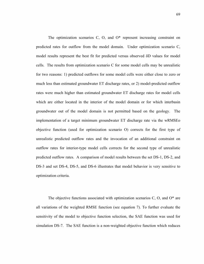
69

The optimization scenarios C, O, and O* represent increasing constraint on

predicted rates for outflow from the model domain. Under optimization scenario C,

model results represent the best fit for predicted versus observed δD values for model

cells. The results from optimization scenario C for some model cells may be unrealistic

for two reasons: 1) predicted outflows for some model cells were either close to zero or

much less than estimated groundwater ET discharge rates, or 2) model-predicted outflow

rates were much higher than estimated groundwater ET discharge rates for model cells

which are either located in the interior of the model domain or for which interbasin

groundwater out of the model domain is not permitted based on the geology. The

implementation of a target minimum groundwater ET discharge rate via the wRMSEo

objective function (used for optimization scenario O) corrects for the first type of

unrealistic predicted outflow rates and the invocation of an additional constraint on

outflow rates for interior-type model cells corrects for the second type of unrealistic

predicted outflow rates. A comparison of model results between the set DS-1, DS-2, and

DS-3 and set DS-4, DS-5, and DS-6 illustrates that model behavior is very sensitive to

optimization criteria.

The objective functions associated with optimization scenarios C, O, and O* are

all variations of the weighted RMSE function (see equation 7). To further evaluate the

sensitivity of the model to objective function selection, the SAE function was used for

simulation DS-7. The SAE function is a non-weighted objective function which reduces

70

the potential overweighting of large errors that may occur with squared error type

functions such as root mean squared error. Simulations DS-3 and DS-7 represent a set of

model runs were all model inputs were identical, the optimization criteria (concentration

only) was the same, and only the objective function used for model optimization was

varied. As shown on Table 12, cell-to-cell flow rates varied by greater than 10,000 acre-

feet/year for 9 out of 28 flowpaths between simulations DS-1 and DS-7. Predicted

groundwater flow rates within Snake Valley were strongly effected, with variations in

flow rate greater than 100,000 acre-feet/year for flows between southern (cell 1) and

central (cell 8), central and northern (cell 14), and northern and northeastern (cell 17)

sub-basins for the DS-1 and DS-7 simulations. Predicted rates of outflow from the model

domain for simulations DS-1 and DS-7 varied by greater than 10,000 acre-feet/year for

seven model cells, including cells associated with Butte Valley (cell 13), Snake Valley

(cells 1, 8, and 17), Spring Valley (cell 15), Tippett Valley (cell 18), and White River

Valley (cell 7).

A comparison of calculated objective functions between simulations DS-1 and

DS-7 (Table 12) shows that when optimized based on concentration only, model results

from simulation DS-1 had a better (lower) calculated wRMSEc, wRMSEo, and SAE

value, while simulation DS-7 yielded a lower wRMSEo* value. This suggests that the

combination of weighting and error-squaring associated with optimization objective

function for simulation DS-1 (wRMSEc) was better able to match predicted δD values to

observed δD values. The lower wRMSEo* value calculated for simulation DS-7 results

71

suggest that using the SAE objective function for model optimization yielded model

results which were less inconsistent with conceptual groundwater flow and ET discharge

assumptions.

The results from the deterministic-sensitivity analysis illustrate how model

performance is strongly affected by optimization criteria and objective function selection.

The inclusion of both concentration (δD values) and groundwater outflow rates as

optimization criteria generates a multiple-objective optimization problem. For the

simulations described above, the multiple-objective problem was translated into a single-

objective problem in the simulations described above by utilizing objective functions

which used weighting terms to combine concentration errors and outflow errors into a

single value. A limitation to this approach is that it may not adequately represent the

multiple-objective optimization problem for which the solution is characteristically non-

unique (Yapo et al., 1998).

Another approach to multiple-objective optimization problems is through the

evaluation of Pareto-optimal solutions, where the model is optimized to generate a set of

model results which represent minima within the objective space of two or more

objective functions. The Multiple-Objective COMplex Evolution (MOCOM) algorithm

is an example of an automated global optimization algorithm for multiple-objective

problems (Yapo et al., 1998). Appendix C presents a comparison of optimization

approaches applied to an eight-cell DSC model comprising a subset of the BARCAS

72

study area basins. Optimization approaches compared include SCE and MOCOM

algorithms, as well as a uniform random search approach.

5.3 Monte Carlo Uncertainty Analyses

The results for the Monte Carlo uncertainty analysis simulations MC-1 through

MC-7 are presented in Table 13 and on Figure 14 as 95-percent confidence intervals for

water budget components. Each of the 1,000 realizations from Monte Carlo simulations

MC-1 through MC-4, MC-6, and MC-7 generated a set of interbasin groundwater flows

and outflows for the model cells. For each cell, the 1,000 simulated interbasin inflows,

interbasin outflows, and outflows from the model domain were sorted in ascending order.

The 26th and 975th values from the sorted results were identified as the lower confidence

limit (LCL) and upper confidence limit (UCL) for the 95-percent confidence interval,

respectively. For simulation MC-5, 740 Monte Carlo realizations were performed and

the LCL and UCL of the 95-percent confidence interval were identified from the 19th and

721st values from the sorted results. In addition to the flow rate information, Table 13

also provides the median results and a statistical summary of the objective function

values which were output by the model during optimization for each realization.

The potential variability in water budget components for the 12 study area basins

is shown on Figure 14. Basin water budgets are presented which include the following

items:

• “Inputs” include recharge from precipitation and interbasin inflow.

73

• “Outputs” include outflow from the model domain, target groundwater ET

discharge rates, and interbasin outflow. Note that groundwater ET rates

are not subtracted from the total outflow from the model domain.

• “Intrabasin flow” is included for hydrographic areas which have been

divided into sub-basins (Snake Valley, Spring Valley, Steptoe Valley, and

White River Valley).

The magnitudes for water budget components show large range, with some basins

not having any water budget component greater than 50,000 acre-feet/year, compared to

Snake Valley, where multiple water budget components may exceed hundreds of

thousands of acre-feet per year. Generally, basin water budgets could be classified into

small, medium and large as follows:

• Basins with small water budgets (no component greater than 50,000 acre

feet/year) include Cave Valley and Tippett Valley. These basins are

characterized by relatively little recharge and interbasin groundwater

inflow.

• Basins with medium water budgets (some components between 50,000

acre-feet/year and 100,000 acre-feet/year) include Butte Valley, Lake

Valley, Little Smoky Valley, Long Valley, Newark Valley, and Spring

Valley. These basins, comprising half of the study area basins, are

characterized by greater potential recharge rates or interbasin groundwater

inflow from other study area basins.

74

• Basins with large water budgets (some components exceeding 100,000

acre-feet/year) include Jakes Valley, Snake Valley, Steptoe Valley, and

White River Valley. These basins all receive potentially large amounts of

interbasin groundwater inflow from one or more other basins.

The two basins with the largest water budget components for simulations are

Snake Valley and White River Valley. These basins are representative of integrators for

multi-basin flow systems predicted by the model for the study area. White River Valley

receives interbasin groundwater inflow from Cave Valley, Jakes Valley, and potentially

Long Valley via Jakes Valley. Snake Valley receives inflow from Spring Valley, Lake

Valley (via Spring Valley), Steptoe Valley (via Lake Valley and Spring Valley), and

potentially Tippett Valley. These multi-basin flow systems constitute groundwater

sources for the Colorado Regional Flow System and the Great Salt Lake Desert Regional

Flow System (Figure 3).

The bars on Figure 14 illustrate that while there is substantial uncertainty

associated with model cells’ water budget components as a function of Monte Carlo

simulation, some sets of model results for individual water budget components are

always greater than zero while others are never greater than zero. Outflows from the

model domain were always tens of thousands of acre-feet/year or greater for southern

White River Valley (cells 5), northeast Snake Valley (cell 17), and northern Steptoe

Valley (cell 20). Interbasin groundwater flow rates were always greater than 1,000 acre-

feet/year between southern Spring Valley and southern Snake Valley (cells 4 to 1),

75

southern Steptoe to Lake Valley (cells 9 to 2), and Jakes Valley to northern White River

Valley (cells 10 to 7). Intrabasin groundwater flows were always hundreds of acre-

feet/year or greater within Snake Valley (cells 1 to 8 to 14 to 17), White River Valley

(cells 7 to 5), and from northern to central Spring Valley (cells 16 to 15). Model-

predicted flow rates were always less than 10 acre-feet/year for southern Steptoe Valley

(cell 9) to Cave Valley and central Spring Valley (cells 3 and 15, respectively) and for

central to northern Steptoe Valley (cell 11 to cell 20) and less than 600 acre-feet/year for

Jakes Valley to Long Valley (cell 10 to cell 19).

Flow directions between model cells 6 (Little Smoky Valley) and 12 (Newark

Valley) and between cells 10 (Jakes Valley) and 19 (Long Valley) were determined by

the model during the optimization process. Flows between these cells are listed in both

“Input” and “Output” categories on the water budget component figure (Figure 14). For

the set of Monte Carlo simulations performed, the model predicted flow to primarily

occur from Long Valley (cell 19) to Jakes Valley (cell 10), as the flow from Jakes Valley

to Long Valley was usually zero or less than about 600 acre-feet/year. Flow direction

between Newark Valley and Little Smoky Valley showed more variability, however the

upper control limits for 95-percent confidence intervals for all Monte Carlo simulations

are greater for flow from Newark valley to Little Smoky Valley than for Little Smoky

Valley to Newark Valley.

76

5.3.1 Water Budget Component Frequency Distributions

The upper and lower limits of the 95-percent confidence intervals provided in

Table 13 and on Figure 14 provide a general description for the ranges of distributions for

model inputs and model-predicted values; however, these summary statistics do not

provide any description for distributions’ shapes. As a method for illustrating the

distributions associated with water budget components, frequency distributions were

developed for Spring Valley. A frequency distribution shows the frequency that a value

falls within a specific bin of values and is a useful tool for approximating a probability

distribution function. Spring Valley was selected as an example basin due to its range in

recharge and discharge rates and its interaction with other model cells via inflow and

outflow.

A water budget component frequency distribution for Spring Valley from Monte

Carlo simulation MC-5 is shown on Figure 15. The frequency distribution includes the

following components:

• total recharge to Spring Valley (sum of recharge rates for cells 4, 15, and

16)

• total groundwater ET discharge (GWET, sum for cells 4, 15, and 16)

• total outflow minus GWET (sum of outflows from model domain minus

the sum of GWET rates for cells 4, 15, and 16)

• total interbasin inflow (sum of inflow rates from cells 2 [Lake Valley] and

9 [southern Steptoe Valley])

77

• total interbasin outflow (sum of outflow rates to cells 1 [southern Snake

Valley], 14 [northern Snake Valley], and 18 [Tippett Valley])

The total for each of these components were calculated for each of the 1,000

realizations, then the frequency distributions for the summed components were

determined.

The shapes for the frequency distributions appear bell-shaped for total GWET and

total interbasin inflow, more uniform for total recharge and total interbasin outflow, and

much narrower for total outflow minus GWET. The reasonably normal-shaped

distribution for total GWET illustrates that when three uniform distributions of GWET

were combined, the resulting total GWET distribution appears more normal than

uniform. This effect is less pronounced for recharge. The frequency distribution also

illustrates that there is more uncertainty (i.e., a wider distribution) associated with

interbasin outflow rates than inflow rates. The relatively narrow distribution and

predominantly negative rates for total outflow minus GWET suggest that for Monte Carlo

simulation MC-5 the optimization objective function (wRMSEo) yielded minimum

GWET discharge rates and that the model does not predict groundwater flow to outside

the model domain from Spring Valley.

5.3.2 Stability of Statistics

The stability of statistics for model results was evaluated by plotting the mean and

95-percent confidence interval about the mean versus realization number for selected

78

model outputs. The 95-percent confidence interval for parameter x about the mean for

realization n, 05.0)( =αnX , is calculated as:

nnstnxnX n

)()()( 1,2/05.0 −= ±≈ αα (17)

where n is the realization number, )(nx is the mean value of x for realizations 1 through

n, 1,2/ −ntα is the Student’s t-statistic, and s(n) is the standard deviation of x for realizations

1 through n.

Plots for the stability of statistics for water budget components for Spring Valley

for Monte Carlo simulation MC-5 are provided in Figure 16 (interbasin inflow), Figure

17 (interbasin outflow), and Figure 18 (outflow from the model domain). Spring Valley

was selected for this example because of its inclusion of all water budget components and

to allow comparison with the water budget component frequency distributions described

in the previous section. The stability plots begin at realization n = 5.

Statistics are consistently stable across the entire 1,000 realization simulation for

inflow from cell 9 (southern Steptoe Valley) to cell 15 (central Spring Valley) and

outflow from the model domain for cell 16 (northern Spring Valley). Small perturbations

in statistics are apparent overt the first 100 realizations for inflow from cell 9 to cell 4

(southern Spring Valley), outflow from cell 15 to cell 18 (Tippett Valley), and outflow

from the model domain for cell 15. Relatively large variability in statistics versus

realization is apparent for inflow from cell 2 (Lake Valley) to cell 4, outflow from cell 4

to cell 1 (southern Snake Valley) and cell 15 to cell 14 (northern Snake Valley), and

79

outflow from cell 4. Statistics for outflow from cell 15 to cell 14 and outflow from to

model domain from cell 4 appear to stabilize relatively quickly, on the order of a few

hundred realizations. Statistics for inflow to cell 2 from cell 4 and outflow from cell 4 to

cell 1 appear to gradually stabilize over the 1,000-realization simulation,; however, a

slight upward trend in the statistics plots are still visible at realization n = 1,000. This

suggests that a greater number of realizations may be necessary to more completely

characterize these components of the water budget.

5.4 Uniqueness of Model Solutions

The Monte Carlo uncertainty analysis results presented and described in Section

5.3 were for simulations MC-1 through MC-7 which included distributions for model

input parameters. Simulation MC-8 differed from the other Monte Carlo simulations by

using the same model inputs for all 1,000 realizations. In this manner, this simulation

evaluated how the starting population of simplex complexes for the SCE algorithm

(determined by a random generator) affects model output. The variability of model

output from this simulation provides an estimate for how non-uniqueness affects the

model solutions.

Table 14 provides the median and upper and lower control limits for the 95-

percent confidence interval for model output parameters for simulation MC-8, similar to

the summary provided in Table 13 for simulations MC-1 through MC-7. A comparison

between the upper and lower control limits of the 95-percent confidence interval provides

80

an indicator for the range of results which are attributable to model uncertainty.

Confidence interval ranges are generally small for model-predicted flowrates between

cells and outflow from the model domain; however, ranges are greater than 1,000 acre-

feet/year for six interbasin or intrabasin (cell-to-cell) flowrates and for outflow rates for

five model cells. Ranges in model-predicted flowrates were greater than 1,000 acre-

feet/year for Lake Valley (cell 2) to southern Spring Valley (cell 4), Little Smoky Valley

(cell 6) to Newark Valley (cell 12), northern White River Valley (cell 7) and Cave Valley

(cell 3) to southern White River Valley (cell 5), and southern Steptoe Valley (cell 9) to

Lake Valley (cell 2) and southern Spring Valley (cell 4). The largest range in cell-to-cell

flow rates is associated with flow from northern to southern White River Valley (cell 7 to

cell 5), where the range in flowrates was about 12,700 acre-feet/year. Ranges in

flowrates out of the model domain are greater than 1,000 acre-feet/year for model cells 3

(Cave Valley), 5 (southern White River Valley), 6 (Little Smoky Valley), 7 (northern

White River Valley), and 12 (Newark Valley), with the largest ranges associated with

southern and northern White River Valley at about 17,800 acre-feet/year and about

12,700 acre-feet/year, respectively.

The sometimes elevated ranges associated with model-predicted results suggest

that the model solution is non-unique with respect to several multi-basin groundwater

flow paths. This effect appears to be most pronounced in association with White River

Valley, where both cell-to-cell flowrates and outflow from the model domain exhibited

relatively large (greater than 10,000 acre-feet/year) variability. The ranges for these

81

model-predicted flowrates are still well below the expected (median) flowrates associated

with intrabasin flow within and outflow from the White River Valley basin.

6. DISCUSSION

The DSC model developed and applied to for this study produced a balanced

water budget which includes groundwater recharge, groundwater ET discharge, and

interbasin groundwater flow components. The study area water budget was evaluated

through the mass-balance modeling of a conservative tracer (deuterium) through a

network of interconnected cells representing basins. Flows between model cells and out

of the model domain were evaluated by varying the optimization criteria of the model to

allow for increasing constraint on discharge predictions. Of the three base BARCAS DSC

modeling runs, results from optimization scenario O appear to be most realistic given the

unrealistic discharge (ET) rates and interbasin flow rates for scenarios C and O*,

respectively, as described in the results section.

Results from the base BARCAS scenario o DSC model suggest that multi-basin

groundwater flow systems discharge from the southern portion of White River Valley and

the northeast portion of Snake Valley, the sub-basins having lowest average

potentiometric surfaces within the study area. The flow system comprising Long Valley,

Jakes Valley, Cave Valley, and White River Valley and discharging from the southern

portion of White River Valley is consistent with the White River Regional Flow System,

which has been described previously (Eakin, 1966; Kirk and Campana, 1990; Thomas et

82

al., 2001). The system comprising the southern portion of Steptoe Valley, Lake Valley,

Spring Valley, and Snake Valley includes components that have been described

previously (e.g., flow from the southern portion of Spring Valley into Snake Valley as

described by Hood and Rush [1965] and Harrill et al. [1988]) as well as new potential

flowpaths, notably flow from the southern portion of Steptoe Valley into Lake Valley and

Spring Valley and flow from Lake Valley into Spring Valley.

The southern portion of Steptoe Valley is an important area because it has the

highest average potentiometric surface within the study area, receives greater than 35,000

acre-feet/year groundwater recharge, and has a relatively low estimated groundwater ET

discharge rate of less than 4,000 acre-feet/year, resulting in about 31,000 acre-feet/year of

excess groundwater input which must be accounted for as interbasin groundwater

outflow. Based on the available δD data for Steptoe Valley, groundwater from the

southern portion of Steptoe Valley (estimated recharge δD range -111 ‰ to -115.5 ‰)

does not appear to travel as intrabasin flow to the central portion of Steptoe Valley where

δD values for recharge (estimated δD = -116.2 ‰ to -118.3 ‰) and the observed δD

value for the cell (δD = -123 ‰) are both isotopically lighter. Groundwater recharge

occurring in the southern portion of Steptoe Valley may travel south and east as

interbasin flow to Lake Valley and the southern portion of Spring Valley, where the

observed δD values (-111 ‰ and -110 ‰, respectively) are isotopically lighter than the

intrabasin recharge occurring to these (sub)basins (approximately -105 ‰ and -108 ‰,

respectively).

83

Rates of groundwater outflow from the study area, calculated as the total outflow

from the model domain minus the groundwater ET rate, are greater than 10,000 acre-

feet/year for the interior sub-basins central Steptoe Valley and central Spring Valley for

scenario o of the base BARCAS DSC model. These elevated outflow rates may indicate

1) groundwater recharge rates are overestimated, 2) groundwater ET rates underestimate

actual discharge, 3) available stable isotope (deuterium) data do not fully characterize

recharge or regional aquifer characteristics, or 4) groundwater discharge occurs in a

manner that is not manifested in available deuterium data for adjacent basins (i.e.,

groundwater discharge occurs as deep underflow or is masked by contributions from

local recharge).

Interbasin groundwater inflow and outflow rates calculated for the base BARCAS

DSC model for optimization scenario O, along with rates from previous estimates are

presented in Figure 19 (inflow) and Figure 20 (outflow). Results from the Monte Carlo

uncertainty analysis for scenario O (simulation MC-2) are shown in Figures 19 and 20 as

error bars on the inflow and outflow rates. Groundwater inflow rates calculated from the

DSC model were generally higher than previous estimates, with inflow rates for Jakes

Valley, Lake Valley, Snake Valley, and Spring Valley being much higher than previously

reported. Groundwater outflow rates calculated from the DSC model are generally

comparable to previous estimates with the exception of Lake Valley, Spring Valley, and

Steptoe Valley, where the DSC model predicted much higher rates than previous studies.

84

These higher outflow rates are reasonable given that the BCM recharge predictions

developed for the BARCAS study the greater than any previously reported values for

Tippett Valley, Spring Valley, Snake Valley, and Steptoe Valley (Welch and Bright, in

review).

The error bars on Figures 19 and 20 illustrate how relatively small changes in

recharge rates or deuterium values can have substantial effects on net basin groundwater

inflow and outflow rates. Historically, most water budgets have been presented with

tabulated discrete entries for water budget components and with little or no discussion of

uncertainties associated with the estimated rates. The modeling presented in this thesis

has attempted to demonstrate the interaction of uncertainty associated with water

components.

As the accounting model integrates data from multiple aspects of the BARCAS

study, and each aspect contributes to the uncertainty for the groundwater flow within the

basins, within the study area, and to adjacent areas, results from the accounting model

have a substantial amount of associated uncertainty. For example, the accounting model

framework was based on an interpreted geology of hydrographic area boundaries and the

regional potentiometric surface which was inferred from relatively few control points.

Model input δD values were calculated from a geochemical database which was sparse

for several areas, and recharge and discharge estimates each have uncertainty associated

with their calculation methods. The Monte Carlo uncertainty analyses presented in this

85

thesis have quantitatively evaluated how potential variability in recharge flux and

groundwater ET rates affect interbasin flows within and out of the study area.

In addition to the Monte Carlo uncertainty analysis results, another indicator of

model uncertainty is provided by inspection of the results for groundwater flow and

discharge rates shown from the deterministic-sensitivity analyses. The variation between

optimization scenarios and recharge δD estimation methods for groundwater flow rates

and patterns within and out of the study show that some regional flow patterns for the

study area predicted by the DSC model change as a result of constraints on groundwater

discharge (ET) rates during model optimization.

The uncertainty analyses illustrated that there is considerable variability

associated with flow rates and flow paths within the study area. Calculated outflow from

the study area also varied; however several basins were predicted to discharge significant

quantities of water from the study area regardless of optimization approach. Based on the

deterministic-sensitivity and Monte Carlo uncertainty analyses White River Valley and

Steptoe Valley discharge at least 10,000 acre-feet/year of groundwater from the study as

interbasin outflow and Snake Valley discharges at least 50,000 acre-feet/year. These

calculated outflows from the model domain represent the water that is excess after

satisfying the estimated groundwater ET discharge rates. The wide variability in

calculated groundwater outflow from the model domain for Spring Valley indicates that

based on the deuterium data and assumed water budget component distributions used in

86

the model, it is uncertain whether groundwater outflow from the study area occurs from

Spring Valley.

While the model does incorporate a driver for achieving minimum outflows under

certain optimization scenarios, there do not exist explicit sinks for water (or tracer)

outside of the study area boundary. For this reason, calculated discharges from the study

result from drivers within the study area, rather than drivers (constraints) at the model

boundaries. For example, Lake Valley is generally predicted to not have significant

outflow from the study area because fluxes of water (and tracer) from this cell are pulled

into southern Spring Valley and southern Snake Valley and there is no “competition”

from outside the study area for Lake Valley’s groundwater. This condition illustrates the

model’s potential limitation for predicting flow to outside the study area.

Butte Valley, the northern portion of Spring Valley, and the southern portion of

Steptoe Valley are “upgradient” cells that do not have potential inflow from any other

model cell. As upgradient cells, the only input to each cell is precipitation recharge,

therefore the observed δD values should equal the recharge δD values. Observed δD

values are about 4 per mil lighter (more negative) than recharge for the southern portion

of Steptoe Valley and about 5 per mil lighter for the northern portion of Spring Valley.

An observed deuterium value for Butte Valley was not calculable because no appropriate

δD data were identified for this basin; however, the observed value for Long Valley,

which is located adjacent and east of Butte Valley, is isotopically lighter than any

recharge δD values for model cells. The differences between observed δD values for

87

these cells compared to recharge δD values suggest that 1) there are errors associated

with the assumed δD values, 2) these cells receive groundwater input from adjacent

model cells, or 3) a different model or set of assumptions is necessary to explain the

observed and recharge δD values.

The variability of results between optimization scenarios for the deterministic and

Monte Carlo simulations illustrate an over-arching issue of model optimization based on

both observed concentrations (δD values) and target outflow rates. While a model that

clearly defines correlation between concentration and outflow has not been developed, it

is reasonable and likely that concentration and outflow influence each other. A

complicated, non-linear relationship between concentration and outflow is a reason that

an inverse problem-type parameter estimation method was chosen for model

optimization. Uncertainties associated with model predictions may be reduced if a

revised model structure is developed which reduces the influence of potential correlation

between concentration and outflow.

7. CONCLUSIONS AND RECOMMENDATIONS

The groundwater accounting model developed for this study met the objective of

evaluating the uncertainty associated with basin and regional groundwater budgets using

available estimates for groundwater recharge and discharge. Additional research could

improve the predictive capability of the model and the interpretation of model results,

88

especially with respect to the uncertainty analysis and for areas with sparse or no

deuterium data for recharge or regional groundwater. The following are

recommendations for future research:

• The DSC model structure could be modified to explicitly include a

specified component for discharge from the model domain (e.g. a

groundwater ET discharge rate) for each mixed cell. Currently, target

groundwater ET discharge rates are used only in objective function

calculations when outflow is included as optimization criteria. Modifying

the model to include a specified discharge component for each mixed cell

would allow for model optimization using a single objective (deuterium

values) compared to the multiple objective optimization used in this study

for scenarios which include target groundwater ET outflows. If modified,

the model should allow for incorporation of variability in groundwater ET

discharge rates via Monte Carlo analyses.

• The distributions for recharge and groundwater ET rates used in the Monte

Carlo analyses could be refined to better reflect spatial and/or temporal

variability in these water budget components. Revisited distributions for

recharge and groundwater ET discharge may also provide an enhanced

understanding of the uncertainty in the regional water budget as a result of

an extended dry period or climate change.

• A more rigorous evaluation of uncertainty associated with recharge δD

values could improve the uncertainty analysis and the resulting description

89

of model sensitivity to assumed recharge δD values. Model uncertainty

related to observed δD values could also be evaluated by incorporating

distributions for cell observed δD values into the Monte Carlo uncertainty

analysis.

• Groundwater samples representative of regional aquifer could be collected

for chemical and isotopic analysis from (sub) basins with no data (Jakes,

Butte, Central Snake Valley) or limited data (Newark Valley, central

Steptoe, southern Steptoe, northeast Snake Valley)

• Additional samples from recharge areas could be collected for chemical

and isotopic analysis. Deuterium data are sparse for multiple recharge

areas, notably the ranges in the northwest corner of the study area

(Needles, Pancake, and Maverick Springs ranges and Butte Mountains),

along the southern portion of the Schell Creek Range, and from eastern

areas (Deep Creek and Confusion ranges).

• The model domain could be expanded to include hydrographic areas

which are adjacent to the boundaries of the current study area. The

expanded model domain could allow for evaluation of the direction and

rates of interbasin groundwater outflow from the current study area.

• Deuterium value inputs or DSC model cell connectivity could be re-

evaluated for the upgradient cells associated with the northern portion of

Spring Valley and the southern portion of Steptoe Valley. For these cells,

the difference between the observed deuterium values for these cells

90

compared the recharge deuterium values indicates that either there are

errors associated with the assumed deuterium values or these cells receive

groundwater input from adjacent model cells.

• Cell input and output fluxes could be checked using chloride data for

samples collected from wells and springs. Assuming there are no mineral

sinks for chloride in the flow system, chloride may acts as another

conservative tracer and could be used to help validate mix ratios predicted

by the deuterium-calibrated DSC model. Possible flowpaths identified for

the DSC model could also be evaluated using a geochemical modeling

program such as NETPATH (Plummer et al. 1991). Geochemical

modeling using NETPATH was completed for a subset of interbasin and

intra basin flowpaths as part of the BARCAS study and the results from

this modeling may help to verify or refute potential groundwater flowpaths

used for the current DSC model.

91

8. REFERENCES

Avon, L. and T.J. Durbin, 1994. Evaluation of the Maxey-Eakin Method for Estimating Recharge to Ground-Water Basins in Nevada. Water Resources Bulletin 30:99-111.

Bedinger, M.S., J.R. Harrill, W.H. Langer, J.M. Thomas, and D.A. Mulvihill. 1985. Maps showing ground-water levels, springs, and depth to ground water, Basin and Range Province, Nevada: U.S. Geological Survey Water-Resources Investigations Report 83-4119-B.

Brothers, K., T.S. Buqo, and J.V. Tracy. 1993. Hydrology and Steady State Ground-water Model of Snake Valley, East-Central Nevada, and West-Central Utah. LVWD Report No. 9.

Brothers, K., T.S. Buqo, J.V. Tracy, M. Stock, C. Bentley, A. Zdon. and J. Kepper. 1993. Hydrology and Steady State Ground-water Model of Cave Valley, Lincoln and White Pine Counties, Nevada. LVWD Report No. 11.

Brothers, K., A.J. Bernholtz, T.S. Buqo, and J.V. Tracy. 1994. Hydrology and Steady State Ground-water Model of Spring Valley, Lincoln and White Pine Counties, Nevada. LVWD Report No. 13.

Calhoun, S.C. 2000. Regional groundwater flow at the Nevada Test Site using stable isotopes and trace element chemistry, M.S. thesis: University of Nevada Reno.

Campana, M.E. 1975. Finite-state models of transport phenomena in hydrologic systems, University of Arizona, Tuscon. PhD Dissertation.

Campana, M.E., W.R. Sadler, N.L. Ingraham and R.L. Jacobson. 1997. A deuterium-calibrated compartment model of transient flow in a regional aquifer system. Tracer Hydrology 97. A. Kranjc: 389-496.

Carroll, R.W.H., Pohll, G.M., Earman, S., and R.L. Hershey. Global optimization of a deuterium calibrated, discrete-state compartment model (DSCM): Application to the eastern Nevada Test Site. in review. Journal of Hydrology.

Carroll, R.W.H. and G.M. Pohll. In press. A User’s Manual for the Discrete-state Compartment Model-Shuffled Complex Evolution (DSCM-SCE). Division of Hydrologic Sciences, Desert Research Institute.

Daly, C., R.P. Nelson and D.L. Phillips. 1994. A Statistical-topographical Model for Mapping Climatological Precipitation over Mountainous Terrain. Journal of Applied Meteorology 33: 140-158.

92

Darling, W.G. and A.H. Bath. 1988. A stable isotope study of recharge processes in the English Chalk. Journal of Hydrology 101: 31-46.

Dettinger, Michael, 1989, Reconnaissance Estimates of Natural Recharge to Desert Basins in Nevada, U.S.A., by Using Chloride-balance Calculations. Journal of Hydrology, 106 (1989) 55-78.

Dingman, S.L. 2002. Physical Hydrology. Prentice-Hall, Inc. Upper Saddle River, New Jersey. 2nd ed.

Drever, J.I. 1997. The Geochemistry of Natural Waters: Surface and Groundwater Environments - 3rd ed. Upper Saddle River, New Jersey, Prentice-Hall, Inc.

Duan, Q., S. Sorooshian, and V. Gupta. 1992. Effective and efficient global optimization for conceptual rainfall-runoff models. Water Resources Research 28(4): 1015-1031.

Eakin, T.E. 1960. Ground-water Appraisal of Newark Valley, White Pine County, Nevada. Nevada Department of Conservation and Natural Resources Ground Water Reconnaissance Series Report No. 1

Eakin, T.E. 1961. Ground-water Appraisal of Long Valley, White Pine and Elko Counties, Nevada. Nevada Department of Conservation and Natural Resources Ground Water Reconnaissance Series Report No. 3

Eakin, T.E. 1962. Ground-water Appraisal of Cave Valley in Lincoln and White Pine Counties, Nevada. Nevada Department of Conservation and Natural Resources Ground Water Reconnaissance Series Report No. 13

Eakin, T.E. 1966. A regional interbasin ground-water system in the White River area, southeastern Nevada. Water Resources Research (2): 251-271.

Eakin, T.E., J.L. Hughes and D.O. Moore, 1967. Water Resources Appraisal of Steptoe Valley, White Pine and Elko Counties, Nevada. Nevada Department of Conservation and Natural Resources Ground Water Reconnaissance Series Report No. 42.

Earman, S. and R. Hershey. In review. Groundwater recharge estimates for basins in south-central Nevada (eastern Nevada Test site and vicinity) developed using a deuterium-calibrated discrete-state compartment model, Division of Hydrologic Sciences, Desert Research Institute.

Epstein, B.J. 2004. Development and Uncertainty Analysis of Empirical Recharge Prediction Models for Nevada’s Desert Basins. Hydrologic Sciences Program, University of Nevada, Reno, Master’s Thesis.

93

Feeney, T.A., M.E. Campana, and R.L. Jacobson. 1987. A Deuterium-Calibrated Groundwater Flow Model of the Western Nevada Test Site and Vicinity, Desert Research Institute Water Resources Center Publication 45057.

Flint, A.L., L.E. Flint, J.A. Hevesi, and J.B. Blainey. 2004. Fundamental Concepts of Recharge in the Desert Southwest: A Regional Modeling Perspective. in: Groundwater recharge in a desert environment: the southwest United States. AGU Water Science and Application 9.

Friedman, I., J.M. Harris, G.I. Smith, and C.A. Johnson. 2002. Stable isotope composition of waters in the Great Basin, United States. 1. Air-mass trajectories. Journal of Geophysical Research, Vol. 107, No. D19, 14 p.

Gat, J.R. 1981. Groundwater, in Stable Isotope Hydrology, Deuterium and Oxygen-18 in the Water Cycle. Ed. J.R. Gat and R. Gonfiantini. Technical Report Series No. 210, pp. 223-240. IAEA, Vienna.

Glancy, P.A., 1968. Water Resources Appraisal of Butte Valley, Elko and White Pine Counties, Nevada. Nevada Department of Conservation and Natural Resources Ground Water Reconnaissance Series Report No. 49.

Hardman, G. 1936. Precipitation Map of Nevada in Nevada Agricultural Experiment Station.

Harrill, J.R. 1971. Water-resources Appraisal of the Pilot Creek Valley Area, Elko and White Pine Counties, Nevada. Nevada Department of Conservation and Natural Resources Ground Water Reconnaissance Series Report No. 56

Harrill, J.R., Gates, J.S., and Thomas, J.M. 1988. Major ground-water flow systems in the Great Basin region of Nevada, Utah, and adjacent states: U.S. Geological Survey Hydrologic Investigations Atlas HA-694-C.

Harrill, J.R., and Prudic, D.E., 1998. Aquifer systems in the Great Basin Region of Nevada, Utah, and adjacent states - Summary report: U.S. Geological Survey Professional Paper 1409-A.

Hershey, R.L., and S.A. Mizell. 1995, Water Chemistry of Spring Discharge from the Carbonate-rock Province of Nevada and California: Desert Research Institute, Water Resources Center, Publication No. 41140, 42 p., 6 appendix.

Hershey, R.L, L. Justet, V.M. Heilweil, P.M. Gardner, B.F. Lyles, S. Earman, J.M. Thomas, and K.W. Lundmark. In press. A Water Chemistry and Water Quality Assessment of Groundwater in the BARCAS Study Area. Division of Hydrologic Sciences, Desert Research Institute.

Hill, M.C. 1998. Methods and guidelines for effective model calibration: U.S. Geological Survey Water-Resources Investigations Report 98-4005: 90 p.

94

Hood, J.W., and F.E. Rush, 1965. Water-resources Appraisal of the Snake Valley Area, Nevada and Utah. Nevada Department of Conservation and Natural Resources Ground Water Reconnaissance Series Report No. 34

Ingraham, N.L., and B.E. Taylor. 1991. Ligth Stable Isotope Systematics of Large-Scale Hydrologic Regimes in California and Nevada. Water Resources Research, 27(1): 77-90.

Karst, G.B., M.E. Campana, and R.L. Jacobson. 1988. A mixing-cell model of the hydrothermal flow system, northern Dixie Valley, Nevada. Transactions, Geothermal Resources Council 12: 167-174.

Katzer, T., and D.J. Donovan. 2003. Surface Water Resources and Basin Water Budget for Spring Valley, White Pine and Lincoln Counties, Nevada. Las Vegas Valley Water District.

Kirk, S.T., and M.E. Campana, 1990. A Deuterium-calibrated Groundwater Flow Model of a Regional Carbonate-alluvial System. Journal of Hydrology, (119) 357-388.

Laczniak, R.J., J.L. Smith, P.E. Elliott, G.A. DeMeo, M.A. Chatigny and G.J Roemer. 2001. Ground-Water Discharge Determined from Estimates of Evapotranspiration, Death Valley Regional Flow System, Nevada and California. U.S. Geological Survey Water-Resources Investigation Report 01-4195.

Maxey, G.B. and T.E. Eakin. 1949. Ground-water in White River Valley, White Pine, Nye, and Lincoln Counties, Nevada. Nevada State Engineer Water Resources Bulletin 8, 59 p.

Mifflin, M.D. 1968. Delineation of ground-water flow systems in Nevada. University of Nevada, Reno, unpublished Doctoral Thesis, 213 p.

Mifflin, M.D. and Hess, J.W. 1979. Regional carbonate flow systems in Nevada. Journal of Hydrology, v.43, p. 217-237.

Natural Resources Conservation Service (NRCS). Climate Narrative for Eastern White Pine County Soil Survey Are, Nevada. Prepared by the NRCS Natioanl Water and Climate Center, Portland, Oregon.

Nichols, W.D. 2000. Regional Ground-water Evapotranspiration and Ground-water Budgets, Great Basin, Nevada, Chapter C. Regional Ground-water Budgets and Ground-water Flow, Eastern Nevada. U.S. Geological Survey Professional Paper 1628, 82 p.

Plummer, L.N., D.L. Prestemon, and D.C. Thorstenson. 1991. An interactive code (NETPATH) for modeling net geochemical reactions along a flow path. U.S. Geological Survey Water-Resources Investigation Report 91-4078.

95

Prudic, D.E., Harrill, J.R., and Burbey, T.J., 1995, Conceptual evaluation of regional ground-water flow in the carbonate-rock province of the Great Basin, Nevada, Utah, and adjacent states: U.S. Geological Survey Professional Paper 1409-D.

Roth, J.G. and M.E. Campana. 1989. A Mixing-cell Model of the Railroad Valley Regional Groundwater Flow System, Central Nevada, Desert Research Institute Water Resources Center Publication 41123.

Rush, F.E. and T.E. Eakin, 1963. Groundwater Appraisal of Lake Valley in Lincoln and White Pine Counties, Nevada. Nevada Department of Conservation and Natural Resources Ground Water Reconnaissance Series Report No. 24.

Rush, F.E. and S.A. Kazmi, 1965. Water Resources Appraisal of Spring Valley, White Pine and Lincoln Counties, Nevada. Nevada Department of Conservation and Natural Resources Ground Water Reconnaissance Series Report No. 33.

Rush, F.E. and D.E. Everett, 1966. Water Resources Appraisal of Little Fish Lake, Hot Creek, and Little Smoky Valleys, Nevada. Nevada Department of Conservation and Natural Resources Ground Water Reconnaissance Series Report No. 38.

Sadler, W.R. 1990. A Deuterium-Calibrated, Discrete-State Compartment Model of Regional Groundwater Flow, Nevada Test Site and Vicinity. Hydrologic Sciences Program. Reno, University of Nevada Reno, Master’ thesis.

Scott, B.R., T.J. Smales, F.E. Rush, and A.S. Van Denburgh. 1971. Nevada's water resources: Nevada Division of Water Resources, Water for Nevada Report 3, 87 p.

Southern Nevada Water Authority. 2006. Southern Nevada Water Authority Clark, Lincoln, and White Pine Counties Groundwater Development Project Draft Conceptual Plan of Development. Prepared for U.S. Bureau of Land Management.

Thomas, J.M., Welch, A.H., and Dettinger, M.D., 1996, Geochemistry and isotope hydrology of representative aquifers in the Great Basin Region of Nevada, Utah, and adjacent states: U.S. Geological Survey Professional Paper 1409-C.

Thomas, J.M., S.C. Calhoun, and W.B. Apambire. 2001. A Deuterium Mass-balance Interpretation of Groundwater Sources and Flows in Southeastern Nevada. Division of Hydrologic Sciences, Desert Research Institute, Publication No. 41169.

Tóth, J.A. 1963. A Theoretical Analysis of Groundwater Flow in Small Drainage Basins. Journal of Geophysical Research, Vol. 68, No. 16

U.S. Geological Survey. 2005. Basin and Range Carbonate Aquifer System Study: U.S. Geological Survey Fact Sheet 2005-3035.

96

U.S. Geological Survey. 2006. National Water Information System (NWISWeb) data available on the World Wide Web, accessed September 12, 2006, at URL http://waterdata.usgs.gov/nv/nwis/nwis.

Watson, P., P. Sinclair and R. Waggoner. 1976. Quantitative Evaluation of a Method for Estimating Recharge to the Desert Basins of Nevada. Journal of Hydrology, 31 (1976) 335-357.

Welch, A.H., and D.J. Bright, ed. In review. Water Resources of the Basin and Range Carbonate Aquifer System in White Pine County, Nevada, and adjacent areas in Nevada and Utah. U.S. Geological Survey Report to Congress.

Zhu, J. In press. BARCAS Project Uncertainty Analysis of Annual Estimates of Ground-Water Discharge.

97

Figure 1. Study Area

98

Figure 2. Regional Groundwater Flow Systems Identified in the Great Basin

Regional Aquifer System Analysis (RASA) Report. Great Basin physiographic province is shown in gray with boundaries of regional flow systems shown as black lines. The regional flow systems associated with the BARCAS study area are shown in green, with the BARCAS study area highlighted dark green.

99

Figure 3. Conceptual Model Showing Local, Deep-Intermediate, and Regional

Groundwater Flow Systems and Water Budget Components for Accounting Model Cells

100

Figure 4. BARCAS Recharge and Groundwater Evapotranspiration (ET) Discharge Estimates for the Study Area

101

Figure 5. Discrete-State Compartment (DSC) Model Components

102

Figure 6. Recharge Deuterium Sample Locations, Inverse Distance Weighted

(IDW) Interpolated Recharge Deuterium Values, and Recharge-Weighted Average Recharge Deuterium Values

103

Figure 7. Regional / Deep-Intermediate Groundwater Deuterium Sample

Locations and DSC Model Calibration (Observed) Deuterium Values

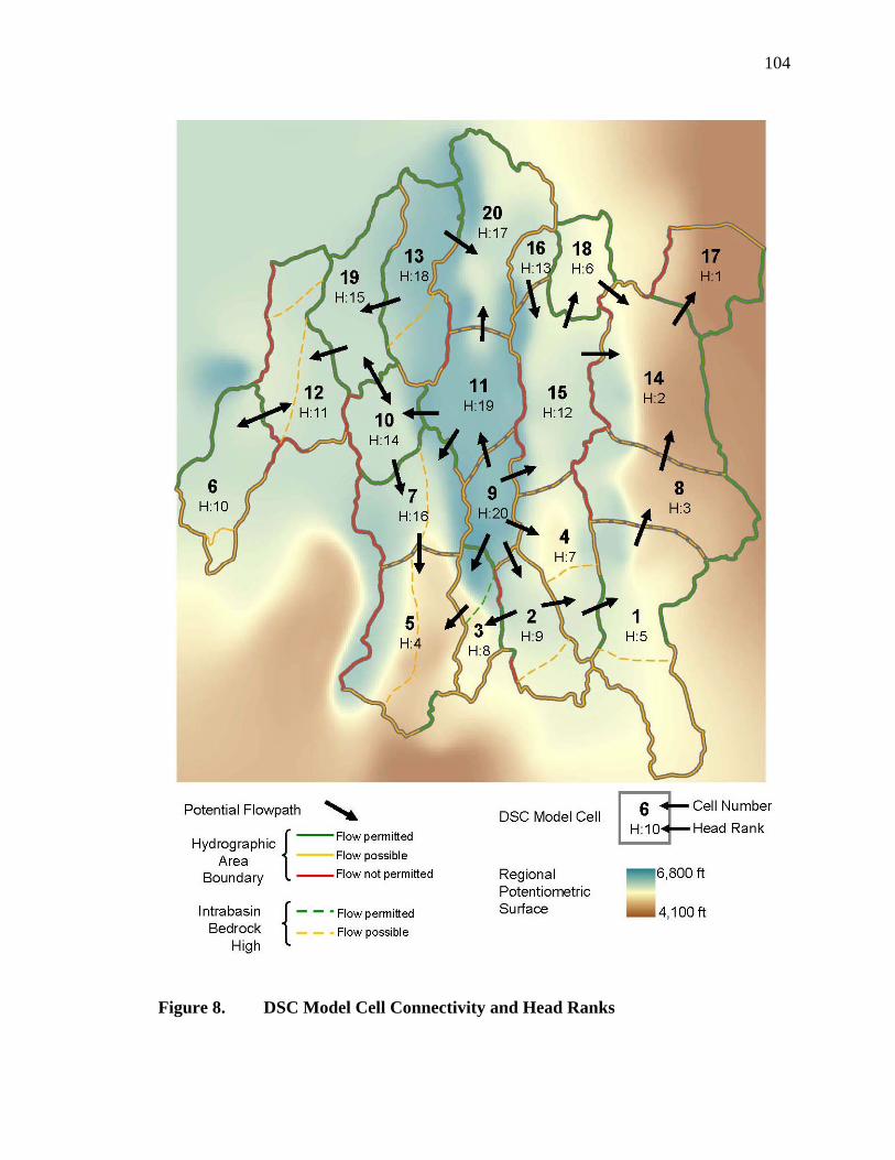
104

Figure 8. DSC Model Cell Connectivity and Head Ranks

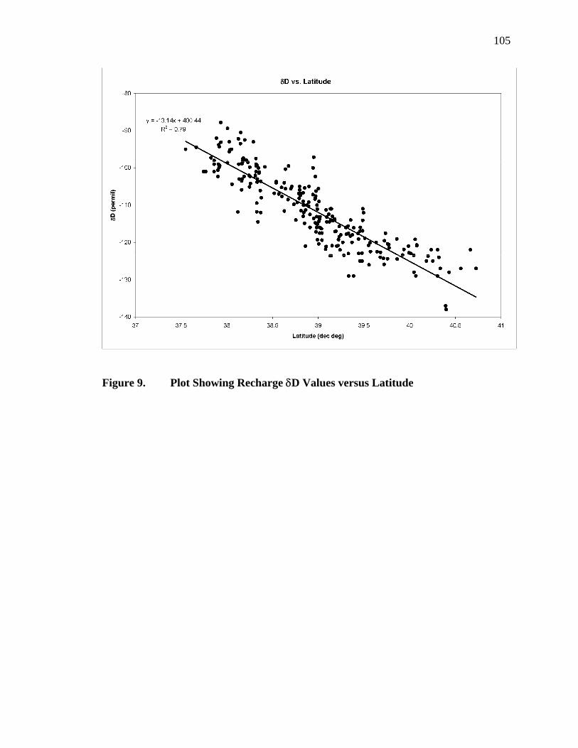
105

Figure 9. Plot Showing Recharge δD Values versus Latitude

106

Figure 10. Ranges of Recharge Estimates Used for Developing Recharge

Distributions for Monte Carlo Uncertainty Analysis Simulations

107

Figure 11. PRISM Map Showing Precipitation Intervals Used for Bootstrap

Brute-Force Recharge Method (BBRM) Recharge Calculations

108

Figure 12. Ranges of Groundwater Evapotranspiration (GWET) Estimates

Used for Developing GWET Distributions for Monte Carlo Uncertainty Analysis Simulations

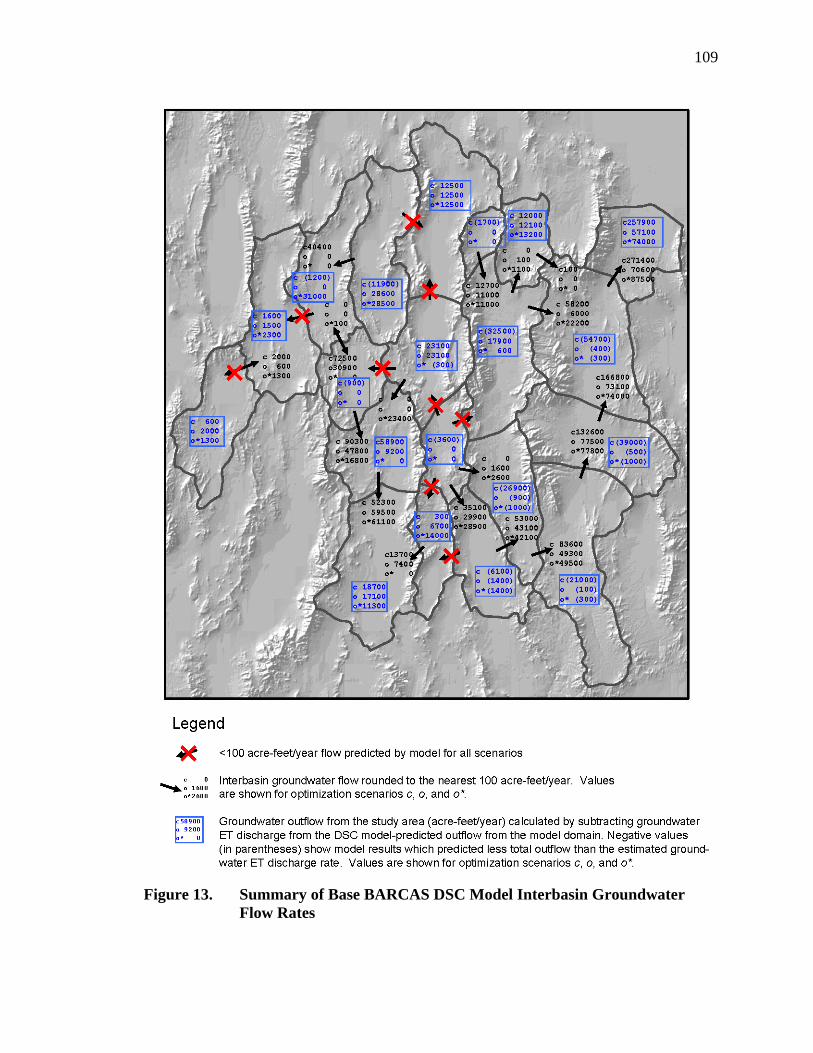
109

Figure 13. Summary of Base BARCAS DSC Model Interbasin Groundwater

Flow Rates

Distributiono

--c

Distributiono

--c

Constanto*

Constanto

--c

Target GWET Rates

Optimization ScenarioSimulation

Figure 14. Water Budget Summary for Monte Carlo Simulations MC-1 through MC-7Hydrographic Area(DSC model cells)

MC-1

MC-2

MC-3

MC-4

MC-5

MC-6

MC-7

DSC model cell network

Monte Carlo Simulations

Notes:Bars show 95% confidence intervalsR = rechargeGWET = groundwater ET dischargeOUT = ouflow from model domain

0

50,000

100,000

150,000

200,000

250,000

300,000

350,000

400,000

R -13

13 -19

13 -20

13 -OU

T

13 -GW

ET

R -3

2 -3

9 -3

3 -5

3 -OU

T

3 -GW

ET

R -10

11 -10

19 -10

10 -7

10 -19

10 -OU

T

10 -GW

ET

R -2

9 -2

2 -3

2 -4

2 -OU

T

2 -GW

ET

R -6

12 -6

6 -12

6 -OU

T

6 -GW

ET

R -19

10 -19

13 -19

19 -10

19 -12

19 -OU

T

19 -GW

ET

R -12

6 -12

19 -12

12 -6

12 -OU

T

12 -GW

ET

R -1

R -8

R -14

R -17

4 -1

15 -14

18 -14

1 -8

8 -14

14 -17

1 -OU

T

1 -GW

ET

8 -OU

T

8 -GW

ET

14 -OU

T

14 -GW

ET

17 -OU

T

17 -GW

ET

R -4

R -15

R -16

2 -4

9 -4

9 -15

16 -15

4 -1

15 -14

15 -18

4 -OU

T

4 -GW

ET

15 -OU

T

15 -GW

ET

16 -OU

T

16 -GW

ET

R -9

R -11

R -20

13 -20

9 -11

11 -20

9 -2

9 -3

9 -4

9 -15

11 -7

11 -10

9 -OU

T

9 -GW

ET

11 -OU

T

11 -GW

ET

20 -OU

T

20 -GW

ET

R -18

15 -18

18 -14

18 -OU

T

18 -GW

ET

R -5

R -7

3 -5

10 -7

11 -7

7 -5

5 -OU

T

5 -GW

ET

7 -OU

T

7 -GW

ET

White River Valley(5, 7)

TippettValley

(18)

Steptoe Valley(9, 11, 20)

Spring Valley(4, 15, 16)

Snake Valley(1, 8, 14, 17)

NewarkValley

(12)

Long Valley(19)

L. SmokyValley

(6)

Lake Valley(2)

Jakes Valley(10)

Cave Valley(3)

ButteValley

(13)

INPU

T

INPU

T

INPU

T

INPU

T

INPU

T

INPU

T

INPU

T

INPU

T

INPU

T

INPU

T

INPU

T

INPU

T

OU

TPUT

OU

TPUT

OU

TPUT

OU

TPUT

OU

TPUT

OU

TPUT

OU

TPUT

OU

TPUT

OU

TPUT

OU

TPUT

OU

TPUT

OU

TPUT

INTR

ABASIN

INTR

ABASIN

INTR

ABASIN

INTR

ABASIN

Acr

e-fe

et/y

ear

110

111

Figure 15. Water Budget Component Distributions for Spring Valley, Monte


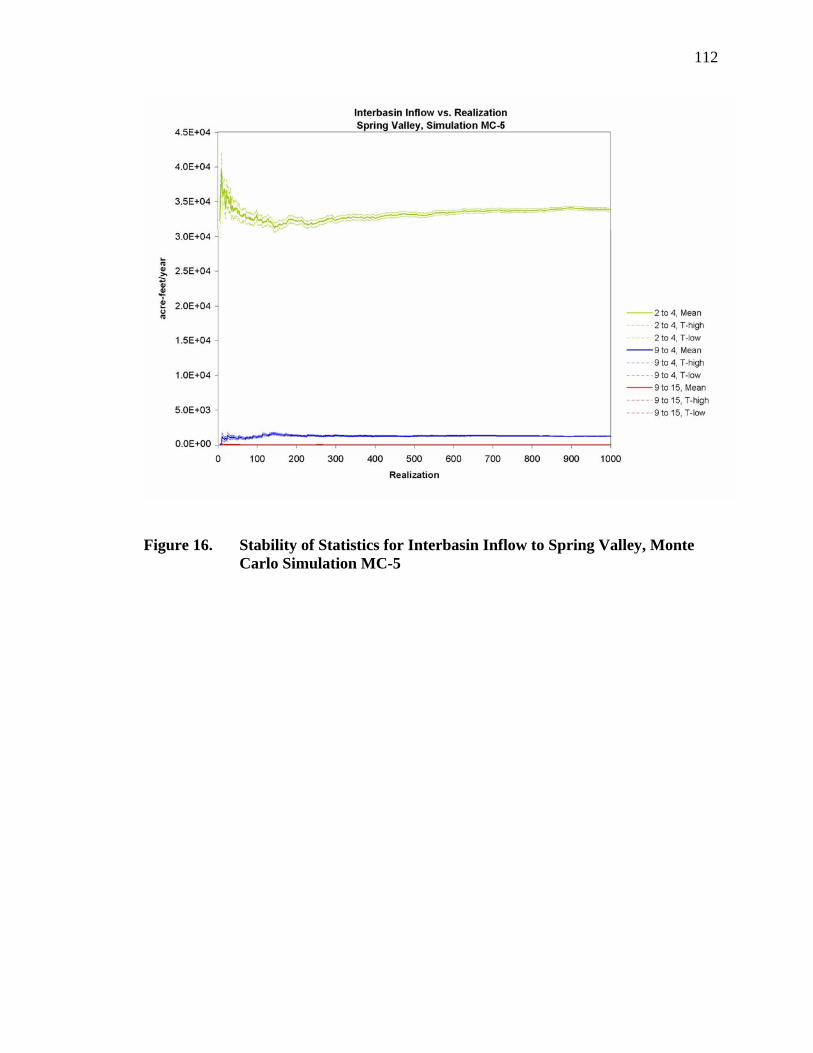
112

Figure 16. Stability of Statistics for Interbasin Inflow to Spring Valley, Monte


113

Figure 17. Stability of Statistics for Interbasin Outflow from Spring Valley,

Monte Carlo Simulation MC-5

114

Figure 18. Stability of Statistics for Outflow from the Model Domain from

Spring Valley, Monte Carlo Simulation MC-5

115

Figure 19. Summary of Interbasin Groundwater Inflow Rates from Previous

Studies and Monte Carlo Simulation MC-2

116

Figure 20. Summary of Interbasin Groundwater Outflow Rates from Previous

Studies and Monte Carlo Simulation MC-2

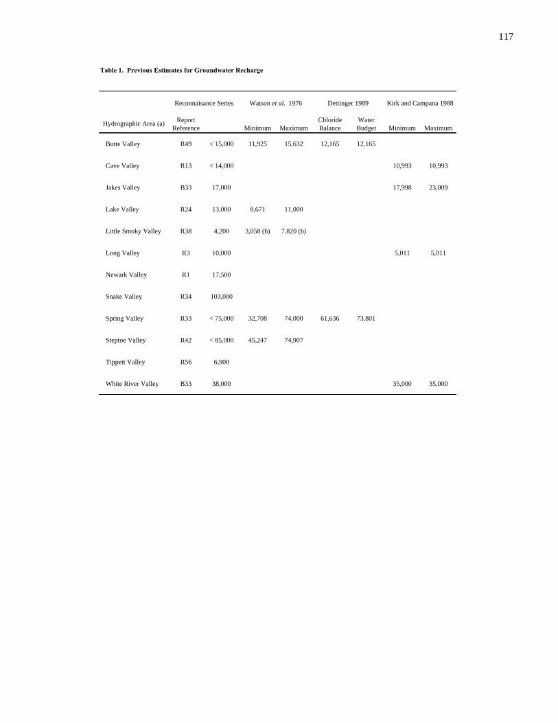
117

Table 1. Previous Estimates for Groundwater Recharge

Report Chloride WaterReference Minimum Maximum Balance Budget Minimum Maximum

Butte Valley R49 < 15,000 11,925 15,632 12,165 12,165

Cave Valley R13 < 14,000 10,993 10,993

Jakes Valley B33 17,000 17,998 23,009

Lake Valley R24 13,000 8,671 11,000

Little Smoky Valley R38 4,200 3,058 (b) 7,820 (b)

Long Valley R3 10,000 5,011 5,011

Newark Valley R1 17,500

Snake Valley R34 103,000

Spring Valley R33 < 75,000 32,708 74,000 61,636 73,801

Steptoe Valley R42 < 85,000 45,247 74,907

Tippett Valley R56 6,900

White River Valley B33 38,000 35,000 35,000

Watson et al. 1976 Dettinger 1989

Hydrographic Area (a)

Reconnaisance Series Kirk and Campana 1988

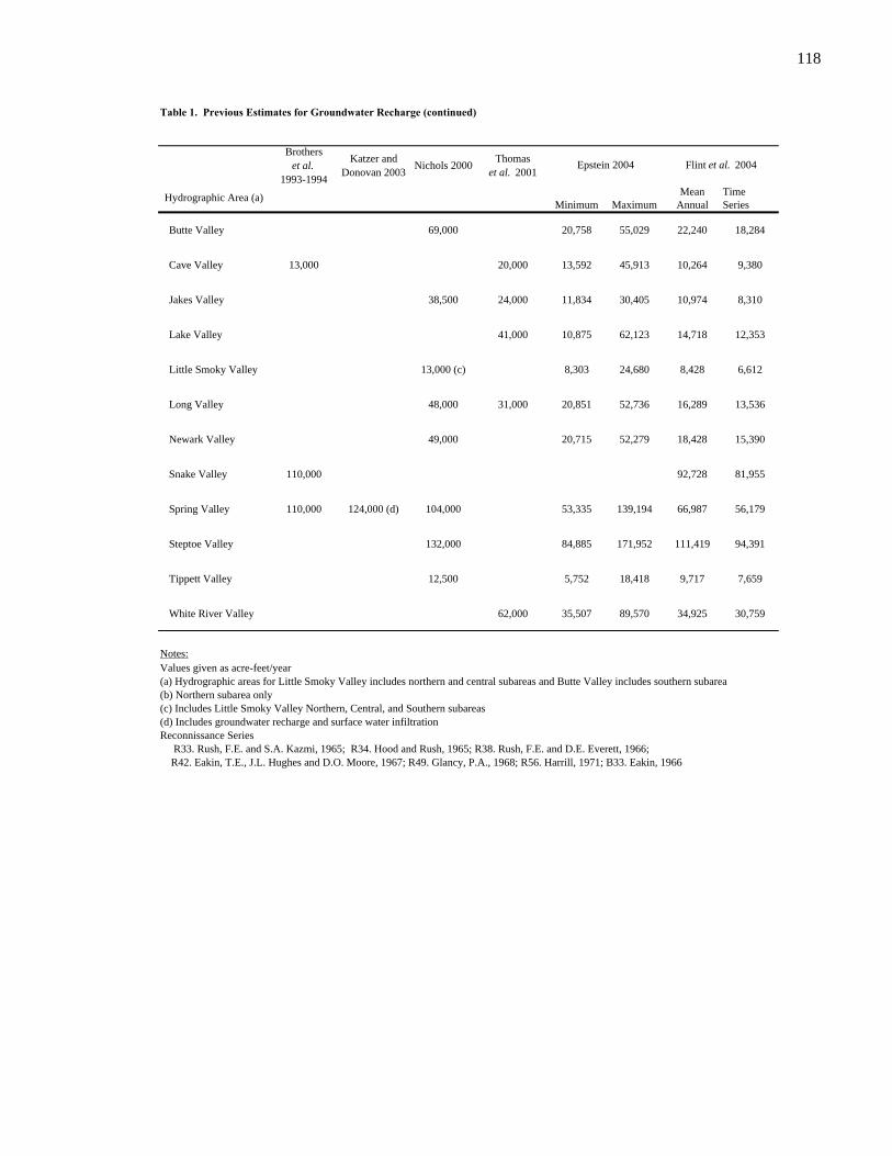
118

Table 1. Previous Estimates for Groundwater Recharge (continued)

Brotherset al.

1993-1994

Katzer andDonovan 2003 Nichols 2000 Thomas

et al. 2001

Mean TimeMinimum Maximum Annual Series

Butte Valley 69,000 20,758 55,029 22,240 18,284

Cave Valley 13,000 20,000 13,592 45,913 10,264 9,380

Jakes Valley 38,500 24,000 11,834 30,405 10,974 8,310

Lake Valley 41,000 10,875 62,123 14,718 12,353

Little Smoky Valley 13,000 (c) 8,303 24,680 8,428 6,612

Long Valley 48,000 31,000 20,851 52,736 16,289 13,536

Newark Valley 49,000 20,715 52,279 18,428 15,390

Snake Valley 110,000 92,728 81,955

Spring Valley 110,000 124,000 (d) 104,000 53,335 139,194 66,987 56,179

Steptoe Valley 132,000 84,885 171,952 111,419 94,391

Tippett Valley 12,500 5,752 18,418 9,717 7,659

White River Valley 62,000 35,507 89,570 34,925 30,759

Notes:Values given as acre-feet/year(a) Hydrographic areas for Little Smoky Valley includes northern and central subareas and Butte Valley includes southern subarea(b) Northern subarea only(c) Includes Little Smoky Valley Northern, Central, and Southern subareas(d) Includes groundwater recharge and surface water infiltrationReconnissance Series R33. Rush, F.E. and S.A. Kazmi, 1965; R34. Hood and Rush, 1965; R38. Rush, F.E. and D.E. Everett, 1966; R42. Eakin, T.E., J.L. Hughes and D.O. Moore, 1967; R49. Glancy, P.A., 1968; R56. Harrill, 1971; B33. Eakin, 1966

Flint et al. 2004Epstein 2004

Hydrographic Area (a)

119

Table 2. Previous Estimates for Groundwater Discharge as Evapotranspiration

Hydrographic Area (a)Report

Reference

Butte Valley R49 11,000 44,500

Cave Valley R13 200 0 5,000

Jakes Valley B33 0 600 600

Lake Valley R24 8,500 24,000

Little Smoky Valley R38 1,900 6,000 (b)

Long Valley R3 2,200 11,000 11,000

Newark Valley R1 18,500 60,500

Snake Valley R34 80,000 87,000

Spring Valley R33 70,000 108,000 (c) 111,000 90,000

Steptoe Valley R42 70,000 128,000

Tippett Valley R56 0 2,900

White River Valley B33 37,000 80,000

Notes:Values given as acre-feet/year(a) Hydrographic areas for Little Smoky Valley includes northern and central subareas and Butte Valley includes southern subarea(b) Includes Little Smoky Valley Northern, Central, and Southern subareas(c) Combination of springflow (drains) and ET

Thomas et al.2001

Reconnissance Series Report References: R1. Eakin 1960; R3. Eakin 1961; R13. Eakin 1962; R24. Rush, F.E. and T.E. Eakin 1963; R33. Rush, F.E. and S.A. Kazmi, 1965; R34. Hood and Rush, 1965; R38. Rush, F.E. and D.E. Everett, 1966; R42. Eakin, T.E., J.L. Hughes and D.O. Moore, 1967; R49. Glancy, P.A., 1968; R56. Harrill, 1971; B33. Eakin, 1966

Reconnaisance Series Brothers et al.1993-1994

Katzer and Donovan

2003

Nichols2000

120

Table 3. Previous Estimates for Interbasin Groundwater Flow

Reconnaissance Series; Harrill et al. 1988 Nichols 2001Interbasin

InflowFromHA

InterbasinOutflow

ToHA

Interbasin Inflow

FromHA

InterbasinOutflow

ToHA

? Steptoe Valley 0 22,500 Clover Valley

2,000 Ruby Valley

Cave Valley 14,000 White River Valley

8,000 Long Valley 25,000 White River Valley 14,000 Long Valley 51,200 White River

Valley

? Railroad Valley 700 Railroad

Valley

Lake Valley 3,000 (a) Patterson Valley

4,000Antelope Valley,Stevens Basin

1,000 (a) Newark Valley 0 1,500 Newark Valley

5,500 Railroad Valley

? Newark Valley 0 10,000 Newark Valley

8,000 Jakes Valley 14,000 Jakes Valley

13,000 Railroad Valley

1,000 (a) Little Smoky Valley ? Railroad

Valley 100,000 Long Valley

? Long Valley 1,500 Little Smoky Valley

4,000 Spring Valley 22,000 - 42,000 Tule Valley 14,000 Spring Valley

< 11,000 Pine Valley ? Fish Springs Flat 3,600 Tippett Valley

< 8,500 Wah Wah Valley 10,000 (a) Great Salt

Lake Desert

2,000 Tippett Valley 4,000 Snake Valley 0 14,000 Snake Valley

Steptoe Valley ? Butte Valley Minor (a) Goshute Valley 0 4,000 Goshute Valley

3,000 Antelope Valley 0 6,000 Great Salt

Lake Desert

2,000

Deep Creek Valley,Great Salt Lake Desert

3,600 Snake Valley

2,000 Spring Valley

14,000 Cave Valley 40,000 Pahroc Valley 51,200 Jakes Valley

25,000 Jakes Valley

Hydrographic Area,

HA (a)

White River Valley

Newark Valley

Snake Valley

Spring Valley

Tippett Valley

Butte Valley

Little Smoky Valley

Jakes Valley

Long Valley

121

Table 3. Previous Estimates for Interbasin Groundwater Flow (continued)

Thomas et al. 2001 Brothers et al. 1993 - 1994 (*), Katzer et al. 2003 (**)Interbasin

InflowFromHA

InterbasinOutflow

ToHA

Interbasin Inflow

FromHA

InterbasinOutflow

ToHA

Cave Valley 0 15,000 Pahroc Valley 0 * 13,000 * White River Valley

12,000 Long Valley 35,000 White River Valley

Lake Valley 0 17,000 Patterson Valley

0 12,000 Jakes Valley

8,000 ?

4,000 * Spring Valley 14,000 * (a)

Great Salt Lake Desert

15,000 * Tule Valley

2,000 * ** Tippett Valley 4,000 *10,000 ** Snake Valley

2,000 ** Steptoe Valley

Steptoe Valley

2,000 * ** Spring Valley

35,000 Long Valley 17,000 Pahroc Valley 13,000 * Cave Valley

Notes:Values given as acre-feet/year(a) Hydrographic areas for Little Smoky Valley includes northern and central subareas and Butte Valley includes southern subarea(b) Flow through alluvial material

Hydrographic Area,

HA (a)

White River Valley

Newark Valley

Snake Valley

Spring Valley

Tippett Valley

1,000 *Pine Valley,Wah Wah

Valley

Butte Valley

Jakes Valley

Little Smoky Valley

Long Valley

122

Table 4. Summary of Groundwater Recharge and Evapotranspiration (ET) Discharge Rate Estimates from the BARCAS Study

Hydrographic Area RechargeET

Discharge

Butte Valley 40,400 11,900

Cave Valley 15,600 1,600

Jakes Valley 17,700 900

Lake Valley 17,900 6,100

Little Smoky Valley 6,600 4,000

Long Valley 32,100 1,200

Newark Valley 27,000 26,100

Snake Valley 133,000 132,300

Spring Valley 103,300 75,600

Steptoe Valley 168,700 101,500

Tippett Valley 13,800 1,700

White River Valley 47,800 76,700

BARCAS Area Total 623,900 439,600

Notes:Source = BARCAS SIR (Welch and Bright, in review)Rates are acre-feet/year (afy), rounded to the nearest 100 afy.

123

Table 5. DSC Model Cell Input Parameters and Calibration Criteria

Cell Name

AverageHead(ft) Rank

Rate(afy)

Deuteriumvalue, δD(‰)

Rate(afy)

Standarddeviation,

s GWET

(afy)

Inversestandard

deviation,1/s GWET

(afy-1)

1 Snake Valley - South 5,596 5 49,082 -107 21,049 4,133 2.4E-04

2 Lake Valley 5,838 9 17,896 -105 6,135 4,438 2.3E-04

3 Cave Valley 5,884 8 15,551 -107 1,551 812 1.2E-03

4 Spring Valley - South 5,780 7 30,579 -108 26,889 4,133 2.4E-04

5 White River Valley - South 5,473 4 15,684 -107 65,463 15,357 6.5E-05

6 Little Smoky Valley 5,935 10 6,562 -121 3,955 545 1.8E-03

7 White River Valley - North 6,114 16 32,129 -113 11,238 1,614 6.2E-04

8 Snake Valley - Central 5,240 3 34,174 -113 39,038 9,404 1.1E-04

9 Steptoe Valley - South 6,543 20 35,140 -114 3,569 371 2.7E-03

10 Jakes Valley 6,055 14 17,691 -119 858 91 1.1E-02

11 Steptoe Valley - Central 6,470 19 64,087 -117 40,983 5,612 1.8E-04

12 Newark Valley 5,962 11 26,986 -122 26,059 5,810 1.7E-04

13 Butte Valley 6,396 18 40,428 -122 11,877 8,682 1.2E-04

14 Snake Valley - North 5,129 2 45,893 -117 54,836 12,432 8.0E-05

15 Spring Valley - Central 5,981 12 59,976 -118 46,991 10,196 9.8E-05

16 Spring Valley - North 6,007 13 12,752 -121 1,733 236 4.2E-03

17 Snake Valley - Northeast 4,480 1 3,851 -122 17,361 6,382 1.6E-04

18 Tippet Valley 5,680 6 13,750 -122 1,742 852 1.2E-03

19 Long Valley 6,091 15 32,130 -123 1,234 1,747 5.7E-04

20 Steptoe Valley - North 6,120 17 69,448 -123 56,945 16,343 6.1E-05

Head Rank Recharge Groundwater ET

124

Table 5. DSC Model Cell Input Parameters and Calibration Criteria (continued)

Cell Name

Deuteriumvalue,δD(‰)

Standard deviation

(‰)

Confidence interval,

ci(‰)

Inverse confidence

interval,1/ci

(‰-1)Weight(‰-1)

1 Snake Valley - South -111 1.60 1.06 0.94 0.94

2 Lake Valley -111 2.26 2.25 0.44 0.44

3 Cave Valley -104 3.16 3.63 0.28 0.28

4 Spring Valley - South -110 2.06 1.45 0.69 0.69

5 White River Valley - South -115 5.63 2.88 0.35 0.35

6 Little Smoky Valley -120 2.22 4.07 0.25 0.25

7 White River Valley - North -120 4.29 3.02 0.33 0.33

8 Snake Valley - Central na -- -- -- 0

9 Steptoe Valley - South -118 3.06 9.29 0.11 0.11

10 Jakes Valley na -- -- -- 0

11 Steptoe Valley - Central -123 0.71 8.98 0.11 0.11

12 Newark Valley -122 nc -- -- 0.1

13 Butte Valley na -- -- -- 0

14 Snake Valley - North -118 4.47 3.37 0.30 0.30

15 Spring Valley - Central -123 1.78 3.27 0.31 0.31

16 Spring Valley - North -126 nc -- -- 0.1

17 Snake Valley - Northeast -111 0.00 0.00 nc 0.5

18 Tippet Valley -122 0.95 2.90 0.34 0.34

19 Long Valley -129 2.12 26.95 0.04 0.1

20 Steptoe Valley - North -128 3.30 2.94 0.34 0.34

Notes:afy = acre-feet/year‰ = per milnc = standard deviation not calculable (less than two δD values for model cell)na = not available (no δD data identified for model cell)

Observed (calibration) values

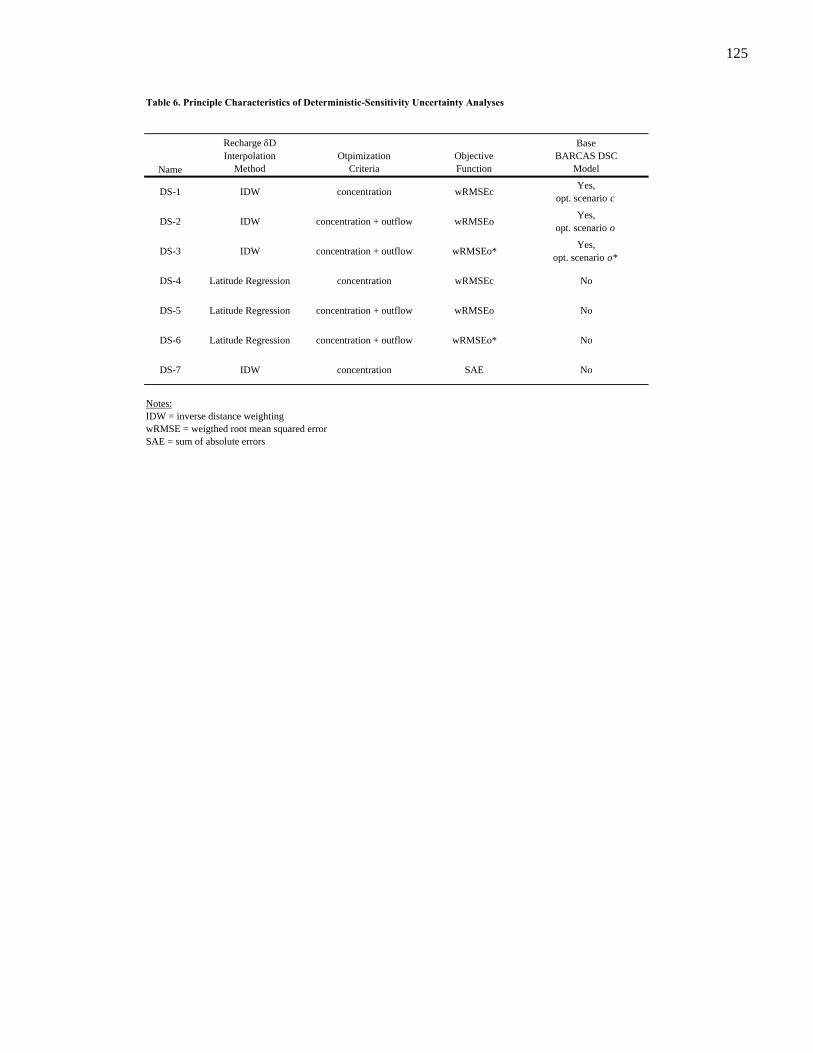
125

Table 6. Principle Characteristics of Deterministic-Sensitivity Uncertainty Analyses

Name

Recharge δDInterpolation

MethodOtpimization

CriteriaObjectiveFunction

BaseBARCAS DSC

Model

DS-1 IDW concentration wRMSEc Yes,opt. scenario c

DS-2 IDW concentration + outflow wRMSEo Yes,opt. scenario o

DS-3 IDW concentration + outflow wRMSEo* Yes,opt. scenario o*

DS-4 Latitude Regression concentration wRMSEc No

DS-5 Latitude Regression concentration + outflow wRMSEo No

DS-6 Latitude Regression concentration + outflow wRMSEo* No

DS-7 IDW concentration SAE No

Notes:IDW = inverse distance weightingwRMSE = weigthed root mean squared errorSAE = sum of absolute errors

126

Table 7. Summary of DSC Model Cell Recharge δD Values Calculated Using Inverse Distance Weighting (IDW) and Latitude Regression Estimation Methods

IDW,δD (‰)

LatitudeRegression,δD (‰)

ΔδD(‰)

1 Snake Valley - South -107 -106 12 Lake Valley -105 -105 03 Cave Valley -107 -106 14 Spring Valley - South -108 -110 -25 White River Valley - South -107 -105 26 Little Smoky Valley -121 -113 87 White River Valley - North -113 -112 18 Snake Valley - Central -113 -112 19 Steptoe Valley - South -114 -112 2

10 Jakes Valley -119 -116 311 Steptoe Valley - Central -117 -117 012 Newark Valley -122 -119 313 Butte Valley -122 -123 -114 Snake Valley - North -117 -118 -115 Spring Valley - Central -118 -117 116 Spring Valley - North -121 -124 -317 Snake Valley - Northeast -122 -122 018 Tippet Valley -122 -123 -119 Long Valley -123 -121 220 Steptoe Valley - North -123 -125 -2

Notes:‰ = per milδD values are rounded to the nearest ‰IDW = inverse distance weightingΔδD = change (Δ) in recharge δD value, calculated by subtracting the Latitude Regression value from the IDW value

DSC Model Cell

Recharge δDEstimation Method

Table 8. Principle Characteristics of Monte Carlo Uncertainty Analysis Simulations

NameOptimization

CriteriaObjectiveFunction

NumberRealizations Distribution

Estimation Methodand Range Distribution

Estimation Methodand Range Distribution Estimation Method Discharge Weight

MC-1 concentration wRMSEc 1,000 UniformBCMMin: IPRMax: IPR + 30% Runoff

Uniform IDW+BCM+/- 1.5 ‰ ananan

MC-2concentration

+ outflow wRMSEo 1,000 UniformBCMMin: IPRMax: IPR + 30% Runoff

Uniform IDW+BCM+/- 1.5 ‰ Constant BARCAS study Constant, 1/sd

MC-3concentration

+ outflow wRMSEo* 1,000 UniformBCMMin: IPRMax: IPR + 30% Runoff

Uniform IDW+BCM+/- 1.5 ‰ Constant BARCAS study Constant, 1/sd

MC-4 concentration wRMSEc 1,000 Quasi-normal BBRM Uniform IDW+BBRM+/- 1.5 ‰ ananan

MC-5concentration

+ outflow wRMSEo 740 Quasi-normal BBRM Uniform IDW+BBRM+/- 1.5 ‰ Quasi-normal BARCAS Monte Carlo

Uncertainty Analysis Variable, 1/(CV*ET)

MC-6 concentration wRMSEc 1,000 Uniform Minimum to Maximumof Avaliable Estimates Uniform Minimum to Maximum

of Avaliable Estimates ananan

MC-7concentration

+ outflow wRMSEo 1,000 Uniform Minimum to Maximumof Avaliable Estimates Uniform Minimum to Maximum

of Avaliable Estimates Uniform Minimum to Maximumof Avaliable Estimates Variable, 1/(CV*ET)

MC-8concentration

+ outflow wRMSEo 1,000 Constant BCMIPR + 15% Runoff Constant IDW+BCM Constant BARCAS study Constant, 1/sd

Notes:IDW = inverse distance weightingwRMSE = weigthed root mean squared errorna = not applicable, outflow not used as optimization criteriaBCM = Basin Characterization ModelBBRM = Bootstrap Brute-force Recharge ModelIPR = Potential in-place rechargeBARCAS study = Basin and Range Carbonate Aquifer studysd = standard deviation

Recharge Rate Recharge δD Values Groundwater ET Discharge Rate

127

128

Table 9. Summary of Recharge δD Values Estimated for DSC Model Cells

1 2 3 4 5 6 7

0% Runoff -106.6 -104.5 -106.5 -108.4 -106.7 -121.4 -113.0

15% Runoff -106.6 -104.6 -107.4 -107.8 -106.7 -121.1 -113.0

30% Runoff -105.5 -103.8 -106.5 -108.0 -106.6 -121.3 -113.2

Minimum -105.5 -103.7 -104.9 -107.9 -107.6 -121.9 -113.7

Average -104.4 -103.6 -104.8 -107.4 -106.6 -121.7 -113.5

Maximum -103.4 -103.6 -104.3 -107.1 -106.2 -121.2 -113.1

0% Runoff -108.3 -104.0 -105.6 -110.1 -105.6 -111.9 -112.5

15% Runoff -107.6 -104.4 -105.8 -110.1 -105.7 -112.0 -112.3

30% Runoff -107.1 -104.6 -106.0 -110.1 -105.7 -112.1 -112.2

Minimum -107.2 -106.0 -106.9 -110.8 -105.5 -115.1 -112.3

Average -105.9 -105.7 -106.6 -109.9 -105.3 -114.1 -112.1

Maximum -104.9 -105.6 -106.5 -109.1 -104.7 -113.6 -112.0

Predicted -105.5 -105.2 -106.1 -109.7 -105.0 -113.5 -111.9

95% CI Lower Limit -106.2 -105.9 -106.8 -110.3 -105.7 -114.1 -112.5

95% CI Upper Limit -104.8 -104.5 -105.4 -109.1 -104.3 -112.9 -111.3

Lower Bound -108.5 -106.25 -107.25 -111 -107.5 -122 -114

Upper Bound -103.5 -103.25 -104.25 -107 -104.5 -112 -111

Thomas et al. 2001 -- -- -107 -- -107 -- -114

Kirk &Campana 1990 -- --

-102to

-97--

-110.5to

-104-- -113

n 40 26 18 36 21 4 42

Average -105.0 -102.1 -106.7 -108.2 -107.5 -123.5 -114.9

Standard Deviation 5.9 5.1 4.6 5.2 5.0 5.0 4.4

DSC Model Cell

Rec

harg

e δD

Est

imat

ion

Met

hods

Use

d fo

rB

asis

of S

elec

ted δ

D R

echa

rge

Ran

ge

IDW + BCM-predicted Spatial

Recharge Distribution

Latitude Regression +

BCM-predicted Spatial Recharge

DistributionLatitude

Regression + BCM-predicted

Spatial Recharge Distribution

IDW + BBRM-predicted Spatial


Latitude Regression x Model Cell

Centroid Latitude

Recharge δD Estimation Method

Rec

harg

e δD

Val

ues

Pres

ente

d fo

r Com

paris

on Recharge δD Values from

Previous Sutdies

Recharge δD Samples within

6.2 miles of Model Cell

SelectedRechargeδD Range

129

Table 9. Summary of Recharge δD Values Estimated for DSC Model Cells (continued)

8 9 10 11 12 13 14

0% Runoff -113.3 -113.6 -118.9 -117.3 -122.4 -122.2 -117.4

15% Runoff -113.1 -113.6 -118.9 -116.5 -121.9 -122.0 -117.2

30% Runoff -112.1 -113.6 -118.9 -117.4 -122.4 -122.1 -117.5

Minimum -111.1 -115.6 -118.9 -118.2 -122.4 -122.2 -118.4

Average -109.7 -113.9 -118.9 -117.7 -122.3 -122.0 -117.5

Maximum -108.5 -113.0 -118.9 -117.3 -122.2 -121.8 -116.8

0% Runoff -111.0 -112.1 -115.1 -118.3 -120.5 -124.4 -119.0

15% Runoff -111.5 -112.1 -115.1 -118.3 -120.2 -124.4 -118.8

30% Runoff -111.8 -112.2 -115.1 -118.3 -120.0 -124.4 -118.7

Minimum -112.9 -113.8 -115.8 -117.0 -120.1 -125.3 -118.8

Average -112.6 -112.6 -115.8 -116.7 -119.6 -124.0 -117.9

Maximum -112.3 -112.0 -115.8 -116.4 -119.2 -123.3 -117.0

Predicted -112.1 -111.7 -115.7 -116.9 -119.4 -122.7 -117.8

95% CI Lower Limit -112.7 -112.3 -116.3 -117.6 -120.2 -123.7 -118.6

95% CI Upper Limit -111.5 -111.1 -115.0 -116.2 -118.6 -121.7 -117.1

Lower Bound -113.5 -115.5 -119 -118.75 -122.5 -125.5 -119.5

Upper Bound -108.5 -111 -115 -115.75 -118.5 -121.5 -116.5

Thomas et al. 2001 -- -- -120 -- -- -- --

Kirk &Campana 1990 -- -- -124 -- -- -- --

n 31 15 26 18 16 14 11

Average -110.6 -111.1 -119.3 -117.1 -122.3 -120.8 -118.5

Standard Deviation 5.1 4.7 4.4 4.4 3.7 3.9 3.4

DSC Model Cell


Rec

harg

e δD

Val

ues

Pres

ente

d fo

r Com

paris


Previous Sutdies



Rec

harg

e δD

Est

imat

ion

Met

hods

Use

d fo

rB

asis

of S

elec

ted δ

D R

echa

rge

Ran

geRecharge δD Estimation Method











Centroid Latitude

130

Table 9. Summary of Recharge δD Values Estimated for DSC Model Cells (continued)

15 16 17 18 19 20

0% Runoff -117.4 -120.9 -120.3 -121.4 -122.4 -122.4

15% Runoff -118.3 -121.4 -122.1 -122.1 -122.7 -122.6

30% Runoff -117.5 -120.9 -120.4 -121.4 -122.4 -122.3

Minimum -117.9 -120.9 -120.4 -121.5 -122.3 -122.4

Average -117.8 -120.9 -120.2 -121.4 -121.8 -122.3

Maximum -117.7 -120.9 -119.8 -121.4 -121.5 -122.3

0% Runoff -116.0 -124.4 -122.0 -123.0 -122.7 -124.8

15% Runoff -116.0 -124.3 -120.2 -122.9 -122.6 -124.8

30% Runoff -116.0 -124.3 -119.8 -122.8 -122.4 -124.7

Minimum -117.5 -123.8 -123.5 -123.9 -122.4 -125.6

Average -117.2 -123.6 -123.4 -123.7 -122.3 -125.2

Maximum -117.0 -123.2 -123.2 -123.6 -122.2 -124.7

Predicted -116.9 -123.7 -122.4 -123.3 -121.0 -124.9

95% CI Lower Limit -117.7 -124.7 -123.3 -124.3 -121.9 -126.0

95% CI Upper Limit -116.2 -122.7 -121.4 -122.3 -120.1 -123.8

Lower Bound -118.5 -124.5 -123.5 -124.5 -123 -126

Upper Bound -115.5 -121 -120 -121.5 -120 -122.5

Thomas et al. 2001 -- -- -- -- -122 --

Kirk &Campana 1990 -- -- -- -- -126 --

n 25 5 0 9 17 10

Average -118.3 -121.3 -- -121.8 -120.3 -122.2

Standard Deviation 3.3 1.4 -- 1.5 4.7 1.4

Notes:Italicized vlues indicate upper and lower bounds calculated as the average of minimum and maximum basis values +/- 1.5‰.Underlined values were used for deterministic-sensitivity analysis simulations; see Tables 6 and 7.

DSC Model Cell


Rec

harg

e δD

Val

ues

Pres

ente

d fo

r Com

paris


Previous Sutdies



Rec

harg

e δD

Est

imat

ion

Met

hods

Use

d fo

rB

asis

of S

elec

ted δ

D R

echa

rge

Ran

geRecharge δD Estimation Method











Centroid Latitude

131

Table 10. Model-Predicted δD Values and Outflow Rates and Calculated Objective Function Values for the Base BARCAS DSC Model

CelldD(‰)

Weight(‰-1) c o o*

Rate(afy)

Weight(afy-1) c o o* c o o*

1 -111 0.94 -109 -108 -108 21,049 0.0002 54 20,912 20,7572 -111 0.44 -111 -111 -111 6,135 0.0002 0 4,759 4,7133 -104 0.28 -107 -107 -107 1,551 0.001 1,893 8,201 15,5524 -110 0.69 -110 -110 -110 26,889 0.0002 1 25,959 25,8635 -115 0.35 -115 -115 -114 65,463 0.00007 84,140 82,601 76,7816 -120 0.25 -121 -121 -121 3,955 0.002 4,588 5,979 5,2227 -120 0.33 -119 -118 -116 11,238 0.0006 70,123 20,421 11,2348 na 0 -110 -110 -110 39,038 0.0001 83 38,558 38,0109 -118 0.11 -114 -114 -114 3,569 0.003 0 3,552 3,552

10 na 0 -122 -122 -119 858 0.01 1 860 85711 -123 0.11 -117 -117 -117 40,983 0.0002 64,061 64,083 40,65812 -122 0.1 -122 -122 -122 26,059 0.0002 27,642 27,593 28,31713 na 0 -122 -122 -122 11,877 0.0001 0 40,427 40,41114 -118 0.30 -113 -113 -113 54,836 0.00008 120 54,443 54,55615 -123 0.31 -119 -118 -118 46,991 0.00010 14,500 64,940 47,63316 -126 0.1 -121 -121 -121 1,733 0.004 2 1,732 1,73317 -111 0.5 -113 -113 -114 17,361 0.0002 275,271 74,444 91,37018 -122 0.34 -122 -122 -122 1,742 0.001 13,715 13,803 14,90719 -129 0.1 -122 -123 -123 1,234 0.0006 1 1,200 32,25020 -128 0.34 -123 -123 -123 56,945 0.00006 69,449 69,460 69,464

All 0.85 0.93 0.98All 4.13 0.08 0.08All 8.97 1.66 0.09All 2.98 0.66 0.70All 6.37 1.35 0.70

Notes:ET - evapotranspirationwRMSE - weighted root mean squared errorDSC model optimization:

c - concentration onlyo - concentration + outflowo* - concentration + modified outflow

Objective function values,wRMSE(unitless)

Predicted deuterium values, δD

(‰)

Predicted outflow rate(acre-ft/year)

Groundwater ET and predicted outflow ratesObserved and predicted deuterium values

Observed (calibration) deuterium values Groundwater ET

Table 11. Basin Water Budget Summary for the Base BARCAS DSC Model

stuptuOstupnIInterbasin Outflow Components

Groundwater Outflow OutflowTotal Interbasin Groundwater Inflow (within study area) (discharge out of study area) Groundwater Outflow - Groundwater ET

Basin Recharge C O O* C O O* C O O* ET C O O*

Butte Valley 40,428 -- -- -- 40,428 1 17 0 40,427 40,411 11,877 (11,876) 28,550 28,534

Cave Valley 15,551 0 0 0 13,658 7,350 0 1,893 8,201 15,552 1,551 342 6,650 14,001

Jakes Valley 17,691 72,544 30,930 0 90,257 47,761 16,833 1 860 857 858 (857) 2 (1)

Lake Valley 17,896 35,140 29,940 28,939 53,036 43,085 42,116 0 4,759 4,713 6,135 (6,135) (1,376) (1,422)

Little Smoky Valley 6,562 0 0 0 72,544 30,930 0 4,588 5,979 5,222 3,955 633 2,024 1,267

Long Valley 32,130 40,427 0 80 1,974 583 1,340 1 1,200 32,250 1,234 (1,233) (35) 31,016

Newark Valley 26,986 1,990 584 1,340 0 0 0 27,642 27,593 28,317 26,059 1,582 1,534 2,258

Snake Valley 133,000 141,895 55,312 71,736 -- -- -- 275,529 188,357 204,693 132,284 143,245 56,073 72,409

Spring Valley 103,306 53,036 44,733 44,766 141,841 55,381 72,850 14,502 92,631 75,229 75,614 (61,111) 17,017 (385)

Steptoe Valley 168,675 0 1 1 35,165 31,592 55,019 133,510 137,095 113,674 101,498 32,012 35,597 12,176

Tippet Valley 13,750 46 69 1,115 100 0 1 13,715 13,803 14,907 1,742 11,973 12,061 13,165

White River Valley 47,813 103,924 55,115 40,199 -- -- -- 154,263 103,022 88,015 76,702 77,561 26,320 11,313

Notes:All values are acre-feet/year(Values in parentheses) indicate negative valuesDSC model optimization:

C - concentration onlyO - concentration + outflowO* - concentration + modified outflow

132

133

Table 12. Summary of Deterministic-Sensitivity Uncertainty Analysis Simulation Results

Simulation: DS-1 DS-2 DS-3 DS-4 DS-5 DS-6 DS-7

IDW IDW IDW Lat. Regr. Lat. Regr. Lat. Regr. IDWObjective Function: wRMSEc wRMSEo wRMSEo* wRMSEc wRMSEo wRMSEo* SAE

Cell to Cell Rates (afy) FromCell

ToCell

1 8 132,610 77,488 77,860 132,650 77,961 78,210 1,4852 3 0 0 0 0 0 0 02 4 53,035 41,783 42,599 53,035 44,657 44,740 53,0093 5 15,122 8,423 1 8,561 1 1 15,4334 1 83,614 49,312 49,546 83,607 49,763 49,903 83,5816 12 588 1,246 118 0 0 0 27 5 55,193 61,448 61,141 72,679 82,006 61,716 77,4348 14 166,750 73,190 74,015 166,640 73,698 74,338 9,5729 2 35,139 28,701 29,382 35,140 31,585 31,585 35,1409 3 0 0 0 0 0 0 09 4 0 2,885 2,204 0 0 2 09 11 0 0 0 0 0 0 09 15 0 0 0 0 0 0 010 7 90,260 47,766 16,790 80,029 37,850 16,833 49,81810 19 0 0 42 0 0 0 011 7 1 3 23,447 7 23,299 23,979 1111 10 11 0 0 5 0 0 011 20 0 1 0 0 0 1 112 6 0 0 0 37,154 11,457 45,691 013 19 40,427 0 0 40,427 0 28,726 013 20 0 4 1 0 4 3 914 17 270,660 70,296 87,699 277,850 72,478 84,963 146,27015 14 58,333 5,679 22,278 61,172 7,350 19,263 72,70715 18 33 8 1,049 3,730 3,511 4,282 016 15 12,752 11,021 11,019 12,752 11,021 11,022 12,75118 14 31 4 0 4,715 7 4 13,62419 10 72,518 30,929 0 62,044 21,050 0 32,12919 12 0 1 1,167 10,506 9,920 59,627 1

Outflow Rates (afy)

Cell

TargetGWET

Rate

TargetGWETWeight

1 21,049 0.0002 86 20,889 20,783 37 20,884 20,785 131,1602 6,135 0.0002 0 4,810 4,669 1 4,819 4,739 273 1,551 0.0012 429 7,129 15,552 6,991 15,551 15,551 1194 26,889 0.0002 1 25,965 25,836 0 25,467 25,406 75 65,463 0.0001 87,017 85,673 76,825 96,312 97,686 77,398 108,4806 3,955 0.0018 5,974 5,316 6,444 43,758 18,023 52,590 6,5607 11,238 0.0006 67,193 18,463 11,231 39,488 11,240 11,216 4,5508 39,038 0.0001 35 38,465 38,056 17 38,433 38,023 27,5449 3,569 0.0027 0 3,554 3,553 0 3,554 3,552 0

10 858 0.0110 4 858 858 1 857 858 111 40,983 0.0002 64,075 64,084 40,640 64,075 40,788 40,107 64,07412 26,059 0.0002 29,763 28,247 29,979 61 25,487 40,483 26,99013 11,877 0.0001 1 40,424 40,427 0 40,424 11,698 40,41914 54,836 0.0001 47 54,431 54,555 25 54,563 54,501 18815 46,991 0.0001 14,359 65,306 47,669 7,825 60,135 47,452 1616 1,733 0.0042 0 1,731 1,733 0 1,731 1,730 117 17,361 0.0002 274,500 74,074 91,582 281,700 76,378 88,779 149,97018 1,742 0.0012 13,749 13,773 14,799 12,658 17,245 18,118 12819 1,234 0.0006 18 1,200 31,006 7 1,160 1,251 020 56,945 0.0001 69,450 69,458 69,457 69,449 69,455 69,453 69,479

Recharge δD Interpolation Method:

134

Table 12. Summary of Deterministic-Sensitivity Uncertainty Analysis Simulation Results (continued)




Predicted δD Values

Cell

ObservedδD Value

(‰)

ObservationWeight(‰-1)

1 -111 0.94 -108.8 -108.3 -108.3 -108.4 -107.9 -107.9 -108.82 -111 0.44 -111.0 -110.5 -110.6 -109.6 -109.5 -109.5 -111.03 -104 0.28 -107.0 -107.0 -107.0 -106.0 -106.0 -106.0 -107.04 -110 0.69 -109.9 -109.6 -109.6 -109.8 -109.7 -109.7 -109.95 -115 0.35 -115.1 -115.0 -113.9 -115.0 -114.2 -112.6 -115.06 -120 0.25 -121.0 -121.0 -121.0 -118.8 -117.2 -120.0 -121.07 -120 0.33 -119.5 -118.1 -115.7 -118.3 -116.0 -114.6 -118.28 na na -109.7 -109.8 -109.8 -109.1 -109.1 -109.1 -112.79 -118 0.11 -114.0 -114.0 -114.0 -112.0 -112.0 -112.0 -114.0

10 na na -121.8 -121.5 -119.0 -120.8 -118.7 -116.0 -121.611 -123 0.11 -117.0 -117.0 -117.0 -117.0 -117.0 -117.0 -117.012 -122 0.10 -121.9 -122.0 -122.1 -119.9 -119.5 -121.0 -122.013 na na -122.0 -122.0 -122.0 -123.0 -123.0 -123.0 -122.014 -118 0.30 -112.8 -112.8 -113.5 -112.8 -112.9 -113.3 -117.815 -123 0.31 -118.5 -118.5 -118.5 -118.2 -118.1 -118.1 -118.516 -126 0.10 -121.0 -121.0 -121.0 -124.0 -124.0 -124.0 -121.017 -111 0.50 -112.9 -113.3 -113.8 -112.9 -113.3 -113.7 -117.918 -122 0.34 -122.0 -122.0 -121.8 -122.0 -122.0 -121.8 -122.019 -129 0.10 -122.4 -123.0 -123.0 -122.1 -121.0 -121.9 -123.020 -128 0.34 -123.0 -123.0 -123.0 -125.0 -125.0 -125.0 -123.0

Objective Function ValueswRMSEc (unitless) 0.85 0.93 0.98 0.87 1.02 1.05 1.08wRMSEo (unitless) 2.98 0.66 0.70 3.11 0.72 0.74 3.02wRMSEo* (unitless) 6.13 1.24 0.70 4.17 0.75 0.74 3.11SAE (‰) 45.22 47.45 51.08 47.08 54.49 52.32 45.71Model Outflow - GWET (afy)

Cell1 -20,963 -160 -266 -21,012 -165 -264 110,1112 -6,135 -1,325 -1,466 -6,134 -1,316 -1,396 -6,1083 -1,122 5,578 14,001 5,440 14,000 14,000 -1,4324 -26,888 -924 -1,053 -26,889 -1,422 -1,483 -26,8825 21,554 20,210 11,362 30,849 32,223 11,935 43,0176 2,019 1,361 2,489 39,803 14,068 48,635 2,6057 55,955 7,225 -7 28,250 2 -22 -6,6888 -39,003 -573 -982 -39,021 -605 -1,015 -11,4949 -3,569 -16 -16 -3,569 -15 -17 -3,56910 -854 0 0 -857 -1 0 -85711 23,092 23,101 -343 23,092 -195 -876 23,09112 3,704 2,188 3,920 -25,998 -572 14,424 93113 -11,876 28,547 28,550 -11,877 28,547 -179 28,54214 -54,789 -405 -281 -54,811 -273 -335 -54,64815 -32,632 18,315 678 -39,166 13,144 461 -46,97516 -1,733 -2 0 -1,733 -2 -3 -1,73217 257,139 56,713 74,221 264,339 59,017 71,418 132,60918 12,007 12,031 13,057 10,916 15,503 16,376 -1,61419 -1,216 -34 29,772 -1,227 -74 17 -1,23420 12,505 12,513 12,512 12,504 12,510 12,508 12,534

135

Table 12. Summary of Deterministic-Sensitivity Uncertainty Analysis Simulation Results (continued)




Net Interbasin Inflow (afy)Butte Valley 0 0 0 0 0 0 0Cave Valley 0 0 0 0 0 0 0Jakes Valley 72,529 30,929 0 62,049 21,050 0 32,129Lake Valley 35,139 28,701 29,382 35,140 31,585 31,585 35,140Little Smoky Valley 0 0 0 37,154 11,457 45,691 0Long Valley 40,427 0 42 40,427 0 28,726 0Newark Valley 588 1,248 1,285 10,506 9,920 59,627 2Snake Valley 141,978 54,996 71,824 149,494 57,120 69,170 169,912Spring Valley 53,035 44,668 44,804 53,035 44,657 44,743 53,009Steptoe Valley 0 4 1 0 4 3 9Tippett Valley 33 8 1,049 3,730 3,511 4,282 0White River Valley 105,383 56,192 40,238 88,596 61,150 40,813 65,262

Butte Valley 40,427 4 1 40,427 4 28,729 9Cave Valley 15,122 8,423 1 8,561 1 1 15,433Jakes Valley 90,260 47,766 16,832 80,029 37,850 16,833 49,818Lake Valley 53,035 41,783 42,599 53,035 44,657 44,740 53,009Little Smoky Valley 588 1,246 118 0 0 0 2Long Valley 72,518 30,930 1,167 72,550 30,970 59,627 32,130Newark Valley 0 0 0 37,154 11,457 45,691 0Snake Valley 0 0 0 0 0 0 0Spring Valley 141,980 54,999 72,873 148,509 60,624 73,448 156,288Steptoe Valley 35,151 31,589 55,034 35,151 54,885 55,567 35,152Tippett Valley 31 4 0 4,715 7 4 13,624White River Valley 0 0 0 0 0 0 0

Outflow from Study Area - BARCAS GWET (afy)Butte Valley -11876 28547 28550 -11877 28547 -179 28542Cave Valley -1122 5578 14001 5440 14000 14000 -1432Jakes Valley -854 0 0 -857 -1 0 -857Lake Valley -6135 -1325 -1466 -6134 -1316 -1396 -6108Little Smoky Valley 2019 1361 2489 39803 14068 48635 2605Long Valley -1216 -34 29772 -1227 -74 17 -1234Newark Valley 3704 2188 3920 -25998 -572 14424 931Snake Valley 142384 55575 72692 149496 57974 69804 176578Spring Valley -61253 17389 -375 -67787 11720 -1025 -75589Steptoe Valley 32028 35599 12153 32027 12300 11615 32056Tippett Valley 12007 12031 13057 10916 15503 16376 -1614White River Valley 77509 27435 11355 59099 32225 11913 36329

Notes:All simulationsBCM-predicted recharge rates assuming 15 percent potential runoff becoming recharge.Underlined values indicate outflow rates for 'interior' model cells for optimization scenario O*.afy = acre-feet/yearwRMSE = weighted root mean square errorSAE = sum of absolute errorsIDW = inverse distance weightingLat. Regr. = latitude regression

Net Interbasin Outflow (in Study Area, afy)

136

Table 13. Summary of Monte Carlo Uncertainty Analysis Results for Simulations MC-1 through MC-7

Median 95% LCI 95% UCI Median 95% LCI 95% UCIRecharge (afy)

Recharge To cellR 1 49,085 42,880 55,250 48,980 42,730 55,400R 2 18,035 14,570 21,300 17,870 14,460 21,310R 3 15,575 14,380 16,710 15,560 14,420 16,720R 4 30,515 26,170 34,930 30,225 26,260 34,920R 5 15,710 15,100 16,270 15,660 15,100 16,270R 6 6,548 6,126 7,001 6,572 6,123 6,998R 7 32,005 29,410 34,840 32,100 29,440 34,840R 8 33,990 28,120 40,250 34,560 28,180 40,300R 9 35,220 33,530 36,780 35,230 33,490 36,750R 10 17,660 16,780 18,600 17,680 16,790 18,600R 11 64,200 59,730 68,500 64,150 59,680 68,560R 12 26,885 24,710 29,290 27,000 24,720 29,250R 13 40,400 38,310 42,610 40,480 38,300 42,570R 14 45,880 41,210 50,570 45,860 41,250 50,570R 15 59,830 50,480 69,400 60,290 50,590 69,440R 16 12,770 11,860 13,640 12,740 11,860 13,620R 17 3,848 1,532 6,124 3,765 1,512 6,123R 18 13,780 12,790 14,700 13,750 12,800 14,710R 19 32,080 30,490 33,730 32,050 30,510 33,760R 20 69,480 64,840 74,030 69,275 64,840 74,080

Cell to Cell Fluxes (afy)From cell To cell

1 8 132,500 122,800 142,500 77,405 67,630 86,9402 3 0 0 1 0 0 12 4 52,375 35,640 57,370 41,580 27,850 48,1003 5 13,540 1,533 16,100 7,370 1,595 12,9404 1 83,740 77,320 90,280 49,340 42,800 55,7606 12 797 0 6,885 890 0 2,6257 5 56,190 34,120 78,650 58,640 48,230 77,8508 14 166,300 154,600 178,100 73,245 61,510 85,1209 2 34,595 19,630 36,770 28,800 17,220 32,9009 3 0 0 0 0 0 09 4 0 0 16,250 2,647 0 14,5409 11 0 0 1 0 0 19 15 0 0 0 0 0 0

10 7 82,330 47,890 92,540 47,750 45,560 49,88010 19 0 0 0 0 0 011 7 8 0 124 7 0 25,98011 10 2 0 142 0 0 011 20 0 0 1 0 0 112 6 0 0 28,700 0 0 2,67313 19 32,825 0 42,410 0 0 013 20 1 0 41,690 3 0 30,64014 17 269,850 236,400 301,300 70,770 53,500 95,76015 14 57,000 27,650 78,090 5,406 1 22,50015 18 73 0 6,281 243 0 6,61416 15 12,770 11,860 13,640 11,000 10,130 11,89018 14 225 6 13,350 5 0 3,93019 10 64,360 30,550 74,960 30,850 29,290 32,57019 12 1 0 35 1 0 9

MC-1 MC-2

137

Table 13. Summary of Monte Carlo Uncertainty Analysis Results for Simulations MC-1 through MC-7 (contd.)

Median 95% LCI 95% UCI Median 95% LCI 95% UCI

MC-1 MC-2

From cell To1 OUT 38 2 326 20,880 20,620 21,0202 OUT 1 0 4 4,858 3,931 5,4843 OUT 1,976 81 13,830 8,122 2,637 13,9604 OUT 1 0 13 25,950 25,130 26,5505 OUT 85,057 51,864 108,170 81,289 72,108 101,3506 OUT 5,659 5 35,260 5,637 3,979 9,1847 OUT 55,760 3,054 86,640 23,100 14,030 39,1808 OUT 42 2 310 38,440 37,550 38,8709 OUT 0 0 0 3,553 3,543 3,561

10 OUT 6 0 99 860 857 87211 OUT 64,080 59,650 68,460 63,175 40,930 68,53012 OUT 29,010 9 35,700 27,670 25,860 30,49013 OUT 10 0 42,300 39,880 11,240 42,52014 OUT 60 2 329 54,470 53,990 54,79015 OUT 13,540 14 45,170 62,660 46,880 78,95016 OUT 1 0 9 1,732 1,730 1,74117 OUT 273,695 240,220 305,370 74,749 56,860 100,23018 OUT 13,825 274 19,630 14,405 10,390 20,40019 OUT 2 0 54 1,200 1,176 1,22320 OUT 70,547 64,932 112,380 70,722 64,855 102,020

From cell To1 GWET -- -- -- 21,049 21,049 21,0492 GWET -- -- -- 6,135 6,135 6,1353 GWET -- -- -- 1,551 1,551 1,5514 GWET -- -- -- 26,889 26,889 26,8895 GWET -- -- -- 65,463 65,463 65,4636 GWET -- -- -- 3,955 3,955 3,9557 GWET -- -- -- 11,238 11,238 11,2388 GWET -- -- -- 39,038 39,038 39,0389 GWET -- -- -- 3,569 3,569 3,569

10 GWET -- -- -- 858 858 85811 GWET -- -- -- 40,983 40,983 40,98312 GWET -- -- -- 26,059 26,059 26,05913 GWET -- -- -- 11,877 11,877 11,87714 GWET -- -- -- 54,836 54,836 54,83615 GWET -- -- -- 46,991 46,991 46,99116 GWET -- -- -- 1,733 1,733 1,73317 GWET -- -- -- 17,361 17,361 17,36118 GWET -- -- -- 1,742 1,742 1,74219 GWET -- -- -- 1,234 1,234 1,23420 GWET -- -- -- 56,945 56,945 56,945

Target Groundwater ET Discharge Rate (afy)

Outflow from Model Domain (afy)

138



MC-1 MC-2

Predicted dD Values (‰)Cell

1 -108.8 -109.7 -107.9 -108.8 -109.7 -107.92 -111.0 -111.5 -109.7 -111.0 -111.5 -109.73 -107.0 -108.4 -105.6 -107.0 -108.4 -105.64 -109.9 -110.9 -108.9 -109.9 -110.9 -108.95 -115.0 -115.1 -114.9 -115.0 -115.1 -114.96 -120.9 -122.3 -119.8 -120.9 -122.3 -119.87 -119.0 -119.9 -118.0 -119.0 -119.9 -118.08 -109.7 -110.5 -108.8 -109.7 -110.5 -108.89 -114.0 -115.4 -112.6 -114.0 -115.4 -112.6

10 -121.8 -122.8 -120.7 -121.8 -122.8 -120.711 -117.0 -118.4 -115.6 -117.0 -118.4 -115.612 -122.0 -123.0 -120.6 -122.0 -123.0 -120.613 -122.0 -123.4 -120.6 -122.0 -123.4 -120.614 -112.8 -112.8 -112.8 -112.8 -112.8 -112.815 -118.5 -119.8 -117.3 -118.5 -119.8 -117.316 -121.0 -122.4 -119.6 -121.0 -122.4 -119.617 -112.9 -113.0 -112.9 -112.9 -113.0 -112.918 -122.0 -122.0 -120.6 -122.0 -122.0 -120.619 -122.8 -124.4 -121.4 -122.8 -124.4 -121.420 -123.0 -124.4 -121.7 -123.0 -124.4 -121.7

Objective Function Values (unitless)wRMSEc 0.87 0.75 1.01 -- -- --wRMSEo -- -- -- 0.67 0.58 0.78wRMSEo* -- -- -- -- -- --

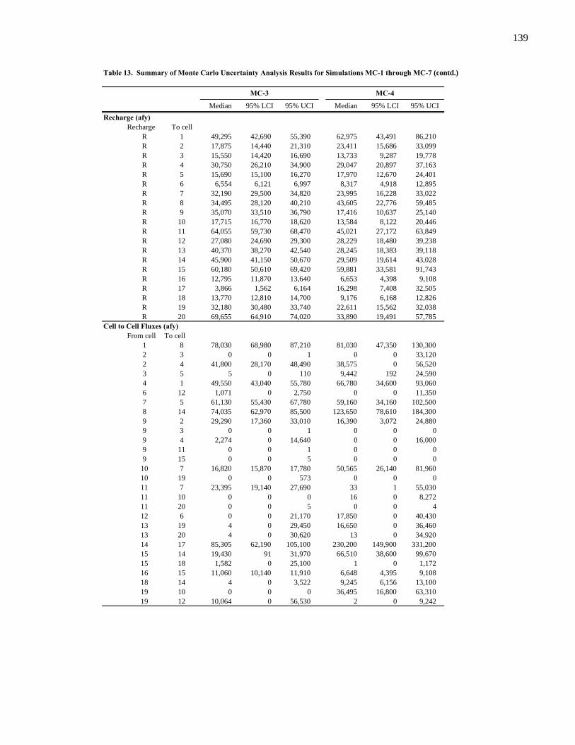
139





1 8 78,030 68,980 87,210 81,030 47,350 130,3002 3 0 0 1 0 0 33,1202 4 41,800 28,170 48,490 38,575 0 56,5203 5 5 0 110 9,442 192 24,5904 1 49,550 43,040 55,780 66,780 34,600 93,0606 12 1,071 0 2,750 0 0 11,3507 5 61,130 55,430 67,780 59,160 34,160 102,5008 14 74,035 62,970 85,500 123,650 78,610 184,3009 2 29,290 17,360 33,010 16,390 3,072 24,8809 3 0 0 1 0 0 09 4 2,274 0 14,640 0 0 16,0009 11 0 0 1 0 0 09 15 0 0 5 0 0 0

10 7 16,820 15,870 17,780 50,565 26,140 81,96010 19 0 0 573 0 0 011 7 23,395 19,140 27,690 33 1 55,03011 10 0 0 0 16 0 8,27211 20 0 0 5 0 0 412 6 0 0 21,170 17,850 0 40,43013 19 4 0 29,450 16,650 0 36,46013 20 4 0 30,620 13 0 34,92014 17 85,305 62,190 105,100 230,200 149,900 331,20015 14 19,430 91 31,970 66,510 38,600 99,67015 18 1,582 0 25,100 1 0 1,17216 15 11,060 10,140 11,910 6,648 4,395 9,10818 14 4 0 3,522 9,245 6,156 13,10019 10 0 0 0 36,495 16,800 63,31019 12 10,064 0 56,530 2 0 9,242

MC-3 MC-4

140



MC-3 MC-4

From cell To1 OUT 20,790 20,530 20,990 45,835 4,547 79,6902 OUT 4,755 3,881 5,416 1 0 29,9303 OUT 15,520 14,360 16,680 5,437 118 36,4704 OUT 25,870 25,090 26,470 1 0 185 OUT 76,786 70,919 83,555 86,496 51,364 140,1606 OUT 5,450 3,987 27,870 21,865 27 48,5507 OUT 11,230 11,210 11,250 21,435 429 78,4708 OUT 38,160 37,250 38,820 177 6 1,3459 OUT 3,553 3,543 3,562 0 0 0

10 OUT 858 857 859 11 0 13011 OUT 40,650 40,280 40,970 40,280 0 62,43012 OUT 34,760 25,880 81,790 4,726 5 44,51013 OUT 39,030 11,210 42,450 7 0 32,45014 OUT 54,550 54,200 54,780 40 2 22415 OUT 47,500 46,890 48,150 7 0 7416 OUT 1,732 1,730 1,735 2 0 1517 OUT 89,399 66,431 109,460 245,990 158,510 360,36018 OUT 15,150 11,840 39,090 15 1 10119 OUT 23,205 1,309 52,890 4 0 9020 OUT 70,970 65,017 102,360 42,514 20,634 81,852

From cell To1 GWET 21,049 21,049 21,049 -- -- --2 GWET 6,135 6,135 6,135 -- -- --3 GWET 1,551 1,551 1,551 -- -- --4 GWET 26,889 26,889 26,889 -- -- --5 GWET 65,463 65,463 65,463 -- -- --6 GWET 3,955 3,955 3,955 -- -- --7 GWET 11,238 11,238 11,238 -- -- --8 GWET 39,038 39,038 39,038 -- -- --9 GWET 3,569 3,569 3,569 -- -- --

10 GWET 858 858 858 -- -- --11 GWET 40,983 40,983 40,983 -- -- --12 GWET 26,059 26,059 26,059 -- -- --13 GWET 11,877 11,877 11,877 -- -- --14 GWET 54,836 54,836 54,836 -- -- --15 GWET 46,991 46,991 46,991 -- -- --16 GWET 1,733 1,733 1,733 -- -- --17 GWET 17,361 17,361 17,361 -- -- --18 GWET 1,742 1,742 1,742 -- -- --19 GWET 1,234 1,234 1,234 -- -- --20 GWET 56,945 56,945 56,945 -- -- --



141



MC-3 MC-4


1 -108.3 -109.3 -107.5 -106.0 -107.0 -105.02 -110.6 -110.9 -109.5 -108.2 -109.5 -104.33 -107.0 -108.4 -105.6 -104.9 -106.4 -103.64 -109.7 -110.7 -108.6 -108.0 -109.7 -106.85 -113.9 -115.0 -113.1 -115.0 -115.1 -114.96 -121.0 -122.3 -119.6 -121.5 -122.9 -120.67 -115.7 -116.8 -114.7 -118.9 -119.8 -117.98 -109.8 -110.7 -108.9 -107.4 -108.2 -106.69 -114.1 -115.4 -112.6 -113.9 -115.4 -112.6

10 -118.9 -120.5 -117.6 -121.1 -122.1 -120.111 -117.0 -118.5 -115.6 -118.0 -119.4 -116.612 -122.1 -123.2 -121.1 -122.0 -123.2 -120.613 -122.0 -123.4 -120.6 -122.0 -123.4 -120.614 -113.3 -114.2 -112.8 -112.5 -112.7 -112.315 -118.5 -119.7 -117.2 -118.2 -119.6 -117.016 -120.9 -122.4 -119.6 -121.0 -122.4 -119.617 -113.7 -114.5 -113.1 -113.0 -113.1 -112.918 -121.5 -122.0 -120.1 -121.0 -122.0 -119.619 -123.0 -124.4 -121.7 -122.1 -123.4 -120.820 -122.9 -124.4 -121.7 -122.2 -123.4 -120.9

Objective Function Values (unitless)wRMSEc -- -- -- 1.38 1.19 1.60wRMSEo -- -- -- -- -- --wRMSEo* 0.71 0.68 0.66 -- -- --

142





1 8 77,245 46,470 116,800 101,400 59,900 152,4002 3 0 0 21,240 0 0 45,8402 4 34,720 0 50,240 33,520 0 68,2103 5 1,551 1 8,899 10,007 741 38,5904 1 40,965 20,410 64,930 59,405 21,430 95,7406 12 1,581 0 6,959 0 0 7,8037 5 49,400 33,900 69,660 64,790 38,040 120,7008 14 85,565 52,820 138,400 140,500 96,870 199,2009 2 14,350 3,378 22,000 18,915 1,242 35,8709 3 0 0 0 0 0 09 4 1 0 11,810 0 0 20,4309 11 0 0 0 0 0 09 15 0 0 0 0 0 0

10 7 34,430 21,840 52,180 80,175 42,540 123,40010 19 0 0 0 0 0 011 7 1,725 0 22,380 16 1 48,66011 10 0 0 0 15 0 6,43211 20 1 0 6 0 0 212 6 0 0 16,930 23,245 0 58,60013 19 0 0 0 28,890 0 66,55013 20 17,145 1 30,230 2 0 47,26014 17 99,075 39,290 203,400 233,650 162,100 317,10015 14 25,790 1,983 58,930 53,095 22,170 92,82015 18 2 0 1,134 1,960 0 7,57916 15 5,177 3,255 7,605 5,574 2,575 8,90218 14 7,917 4,682 11,950 9,125 2 19,76019 10 21,645 14,150 31,820 57,200 33,070 62,94019 12 3 0 3,818 150 2 9,300

MC-5 MC-6

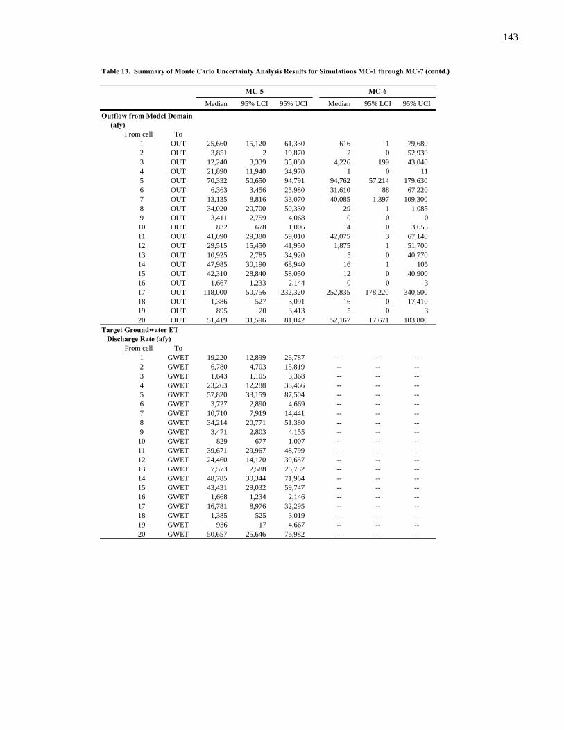
143



MC-5 MC-6

From cell To1 OUT 25,660 15,120 61,330 616 1 79,6802 OUT 3,851 2 19,870 2 0 52,9303 OUT 12,240 3,339 35,080 4,226 199 43,0404 OUT 21,890 11,940 34,970 1 0 115 OUT 70,332 50,650 94,791 94,762 57,214 179,6306 OUT 6,363 3,456 25,980 31,610 88 67,2207 OUT 13,135 8,816 33,070 40,085 1,397 109,3008 OUT 34,020 20,700 50,330 29 1 1,0859 OUT 3,411 2,759 4,068 0 0 0

10 OUT 832 678 1,006 14 0 3,65311 OUT 41,090 29,380 59,010 42,075 3 67,14012 OUT 29,515 15,450 41,950 1,875 1 51,70013 OUT 10,925 2,785 34,920 5 0 40,77014 OUT 47,985 30,190 68,940 16 1 10515 OUT 42,310 28,840 58,050 12 0 40,90016 OUT 1,667 1,233 2,144 0 0 317 OUT 118,000 50,756 232,320 252,835 178,220 340,50018 OUT 1,386 527 3,091 16 0 17,41019 OUT 895 20 3,413 5 0 320 OUT 51,419 31,596 81,042 52,167 17,671 103,800

From cell To1 GWET 19,220 12,899 26,787 -- -- --2 GWET 6,780 4,703 15,819 -- -- --3 GWET 1,643 1,105 3,368 -- -- --4 GWET 23,263 12,288 38,466 -- -- --5 GWET 57,820 33,159 87,504 -- -- --6 GWET 3,727 2,890 4,669 -- -- --7 GWET 10,710 7,919 14,441 -- -- --8 GWET 34,214 20,771 51,380 -- -- --9 GWET 3,471 2,803 4,155 -- -- --

10 GWET 829 677 1,007 -- -- --11 GWET 39,671 29,967 48,799 -- -- --12 GWET 24,460 14,170 39,657 -- -- --13 GWET 7,573 2,588 26,732 -- -- --14 GWET 48,785 30,344 71,964 -- -- --15 GWET 43,431 29,032 59,747 -- -- --16 GWET 1,668 1,234 2,146 -- -- --17 GWET 16,781 8,976 32,295 -- -- --18 GWET 1,385 525 3,019 -- -- --19 GWET 936 17 4,667 -- -- --20 GWET 50,657 25,646 76,982 -- -- --



144



MC-5 MC-6


1 -105.4 -106.4 -104.3 -107.5 -108.4 -105.82 -107.7 -109.1 -104.4 -108.0 -109.7 -104.83 -104.9 -106.4 -103.6 -105.3 -106.3 -104.34 -107.5 -108.8 -106.4 -109.3 -110.1 -107.85 -115.0 -115.1 -113.4 -115.0 -115.0 -114.96 -121.8 -123.2 -120.6 -119.8 -120.0 -118.77 -118.0 -119.0 -117.0 -119.0 -119.6 -117.98 -107.1 -108.0 -106.1 -108.4 -109.1 -107.19 -114.0 -115.4 -112.6 -112.7 -114.2 -111.1

10 -120.8 -122.0 -119.7 -121.2 -121.8 -119.911 -118.0 -119.4 -116.6 -116.9 -118.0 -115.812 -122.1 -123.3 -120.6 -120.6 -121.6 -119.113 -122.0 -123.4 -120.6 -123.0 -124.4 -121.614 -112.0 -112.6 -111.3 -112.4 -112.6 -111.815 -118.3 -119.5 -116.9 -117.3 -118.2 -116.116 -121.0 -122.4 -119.6 -122.4 -123.6 -121.117 -113.1 -114.2 -112.9 -113.0 -113.3 -112.918 -120.9 -122.0 -119.6 -122.0 -122.0 -121.519 -122.0 -123.4 -120.6 -123.0 -123.8 -121.820 -122.2 -123.4 -120.8 -124.0 -125.0 -122.6

Objective Function Values (unitless)wRMSEc -- -- -- 1.09 0.95 1.41wRMSEo 1.09 0.93 1.26 -- -- --wRMSEo* -- -- -- -- -- --

145


Median 95% LCI 95% UCIRecharge (afy)

Recharge To cellR 1 63,090 39,590 84,660R 2 25,725 9,664 40,520R 3 13,800 8,230 19,620R 4 24,450 12,720 36,520R 5 19,280 13,030 25,900R 6 8,064 3,275 12,670R 7 25,805 16,690 34,940R 8 39,370 21,090 58,690R 9 22,745 9,000 36,330R 10 22,975 8,692 37,580R 11 46,030 22,650 67,670R 12 31,370 13,800 48,310R 13 40,175 13,330 67,840R 14 30,545 18,070 42,640R 15 56,770 20,740 89,510R 16 5,794 2,604 8,941R 17 19,685 7,236 31,450R 18 9,924 5,324 14,510R 19 32,090 30,470 33,780R 20 45,345 16,740 73,070


1 8 71,895 38,230 111,4002 3 0 0 20,9402 4 35,470 2 60,3603 5 14 0 12,6504 1 33,370 1,337 64,2106 12 0 0 9,0947 5 62,970 40,630 90,0408 14 74,630 38,930 120,0009 2 16,455 2,181 31,8509 3 0 0 09 4 1 0 12,8409 11 0 0 9,6579 15 0 0 1

10 7 43,820 21,400 63,40010 19 0 0 111 7 42 0 28,71011 10 0 0 011 20 0 0 912 6 1,155 0 26,46013 19 0 0 20,64013 20 12,180 0 50,76014 17 73,600 37,740 136,90015 14 10,960 0 49,19015 18 937 0 5,81516 15 4,067 818 7,25318 14 6,565 1 16,32019 10 23,900 0 31,66019 12 4,856 0 45,980

MC-7

146


Median 95% LCI 95% UCI

MC-7

From cell To1 OUT 22,005 13,610 42,5002 OUT 5,428 0 32,0703 OUT 12,535 2,171 33,4104 OUT 26,600 12,950 40,2205 OUT 84,990 59,601 112,4306 OUT 7,506 2,211 34,4707 OUT 11,765 7,343 26,9108 OUT 37,225 22,090 52,0909 OUT 3,559 2,865 4,206

10 OUT 818 618 1,01711 OUT 38,855 27,030 63,62012 OUT 37,955 16,080 55,34013 OUT 20,950 2,748 63,04014 OUT 51,565 31,570 72,58015 OUT 42,670 24,570 64,55016 OUT 1,732 1,287 2,15717 OUT 93,580 49,172 160,42018 OUT 3,073 132 16,49019 OUT 2,781 6 7,26620 OUT 60,166 31,122 99,286

From cell To1 GWET 21,733 13,677 29,1382 GWET 14,071 5,272 23,5283 GWET 2,409 150 4,8754 GWET 28,615 13,390 44,2615 GWET 66,619 31,970 102,2206 GWET 3,989 2,016 5,8907 GWET 11,113 7,282 14,8998 GWET 39,769 22,612 56,4079 GWET 3,605 2,891 4,262

10 GWET 817 613 1,01311 GWET 40,720 31,158 51,92012 GWET 38,062 15,699 59,32913 GWET 23,805 3,976 43,22814 GWET 55,016 32,228 77,76715 GWET 48,607 30,529 67,40016 GWET 1,736 1,287 2,16717 GWET 21,809 9,589 32,84018 GWET 1,830 90 3,60619 GWET 5,519 256 10,69520 GWET 57,685 29,105 90,926



147


Median 95% LCI 95% UCI

MC-7


1 -107.0 -108.6 -105.12 -108.3 -110.8 -104.83 -105.7 -107.2 -104.34 -108.7 -110.5 -106.95 -114.5 -115.0 -112.46 -118.6 -121.6 -114.77 -117.2 -118.8 -115.28 -108.4 -110.2 -106.69 -113.2 -115.4 -111.1

10 -120.0 -122.2 -117.011 -117.2 -118.7 -115.612 -120.9 -122.7 -118.813 -123.5 -125.4 -121.614 -112.6 -114.4 -110.615 -117.4 -118.9 -116.016 -122.8 -124.4 -121.117 -114.3 -116.6 -112.818 -122.0 -123.8 -121.619 -123.0 -122.5 -123.620 -124.2 -125.8 -122.6

Objective Function Values (unitless)wRMSEc -- -- --wRMSEo 0.93 0.71 1.21wRMSEo* -- -- --

Notes:afy = acre-feet/yearLCI = lower confidence intervalUCI = upper confidence itervalwRMSE = weighted root mean square error

148

Table 14. Summary of Monte Carlo Uncertainty Analysis Results for Simulation MC-8

Median 95% LCI 95% UCICell to Cell Fluxes (afy)

From cell To cell1 8 77,490 77,420 77,5602 3 0 0 12 4 41,710 40,600 43,2603 5 6,975 4,160 9,1004 1 49,310 49,240 49,3706 12 767 212 1,4327 5 58,215 51,090 63,7608 14 73,175 73,080 73,2709 2 28,620 27,640 30,1009 3 0 0 09 4 2,964 1,485 3,9439 11 0 0 09 15 0 0 010 7 47,770 47,750 47,78010 19 0 0 011 7 6 0 2011 10 0 0 011 20 0 0 112 6 0 0 013 19 0 0 013 20 2 0 714 17 70,380 70,040 70,71015 14 5,840 5,557 6,13715 18 48 7 9216 15 11,020 11,020 11,02018 14 4 0 2519 10 30,930 30,920 30,95019 12 1 0 4

From cell To1 OUT 20,900 20,860 20,9302 OUT 4,799 4,740 4,8473 OUT 8,577 6,451 11,3904 OUT 25,950 25,920 25,9905 OUT 80,866 70,761 88,5286 OUT 5,795 5,130 6,3507 OUT 21,685 16,150 28,8208 OUT 38,490 38,420 38,5509 OUT 3,553 3,550 3,55610 OUT 859 857 86511 OUT 64,080 64,070 64,09012 OUT 27,760 27,220 28,42013 OUT 40,430 40,420 40,43014 OUT 54,430 54,270 54,61015 OUT 65,110 64,800 65,40016 OUT 1,732 1,730 1,73517 OUT 74,175 73,809 74,60618 OUT 13,800 13,760 13,86019 OUT 1,195 1,184 1,20720 OUT 69,454 69,449 69,463

Objective Function Values (unitless)wRMSEo 0.662 0.662 0.662

Notes:afy = acre-feet/yearLCI = lower confidence intervalUCI = upper confidence itervalwRMSE = weighted root mean square error

MC-8


149

Appendix A. Deuterium Data for Recharge Samples

NWIS Site Number Site NameLatititude(NAD83)

Longitude(NAD83) Site Type

SampleDate

Deuterium, δD(‰)

9415515 WATER CANYON CREEK NEAR PRESTON, NV 38.98772 -114.95835 SW 10/24/2003 -109.510/24/2003 -112.7

10243740 MCCOY CREEK NEAR MCGILL, NV 39.37411 -114.52834 SW 5/28/1992 -118

373255114102301 204 S05 E70 04BA 1 37.54858 -114.17387 GW 6/3/1985 -95

373953113400801 (C-36-16)20abb- 2 37.66470 -113.66969 GW 1/1/1981 -94.5

374441114252801 203 S02 E67 25DABB1 37.74469 -114.42527 GW 6/4/1985 -101

374607114242501 203 S02 E68 18DD 1 37.76858 -114.40777 GW 6/4/1985 -101

374934114555201 181 S01 E63 33 1 RATTLESNAKE SPRING 37.82608 -114.93111 Spring 3/24/2004 -97.3

375136114192001 198 S01 E68 13DB 1 Spring 37.85996 -114.32304 Spring 4/8/1985 -984/8/1985 -104

375140114191801 198 S01 E68 13 1 MVW above Delmue Spring 37.86107 -114.32249 SW 4/8/1985 -98

375140115115601 171 S01 E60 13 1 SEAMAN SPRING 37.86119 -115.19878 Spring 6/25/2004 -99

375310114181701 198 S01 E69 06DB 1 37.88607 -114.30554 GW 6/5/1985 -92

375406114333701 202 N01 E66 34 1 CONNOR SPRING 37.90164 -114.56022 Spring 6/24/2004 -100.6

375410114333801 202 N01 E66 34ACD 1 BIG TREES SPRING 37.90274 -114.56139 Spring 6/24/2004 -102.3

375429114325601 202 N01 E66 35BB 1 PINE SPRING 37.90802 -114.54972 Spring 4/7/1985 -996/24/2004 -99

375443114550501 181 N01 E63 28CC 1 BLACK ROCK SPRING 37.91190 -114.91890 Spring 3/22/1988 -943/23/2004 -93.6

375452114322501 203 S01 E66 26 1 LIME SPRING 37.91441 -114.54111 Spring 6/24/2004 -99.9

375501114550701 181 N1 E63 28 1 UNNAMED SPRING--NR BLACKROC 37.91694 -114.91861 Spring 3/23/2004 -94.3

375507114322901 202 N01 E66 26AD 1 DEADMAN SPRING 37.91857 -114.54222 Spring 3/23/2004 -86.93/23/2004 -88.7

375516114325601 202 N01 E66 26BAC 1 HIGHLAND SPRING 37.92107 -114.54972 Spring 6/24/2004 -99.65/1/2005 -99.3

375609114531601 181 N01 E63 22 1 HAMILTON SPRING 37.93572 -114.88764 Spring 3/23/2004 -93.1

380022114052301 201 N02 E70 25 1 TOBE SPRING 38.00608 -114.08981 Spring 5/20/2004 -98.6

380024114052301 201 N02 E70 25 1 TOBE SPRING 2 38.00675 -114.08969 Spring 5/20/2004 -89.4

380136114144201 200 N02 E69 15 1 HORSETHIEF SPRING 38.02675 -114.24503 Spring 5/20/2004 -93.75/1/2005 -97.6

380140114110901 201 N02 E70 18C 1 MVW above Eagle Canyon R 38.02774 -114.18665 SW 4/9/1985 -93

380155114514401 181 N02 E63 13 1 COYOTE SPRING 38.03186 -114.86219 Spring 5/1/2005 -95.2

380300115364201 172 N02 E57 07 1 Spring 38.04994 -115.61253 Spring 7/31/1985 -95

380324115395301 172 N02 E56 10 1 UNNAMED SPRING 8 38.05667 -115.66472 Spring 7/2/2005 -104.4

380714114200001 202 N03 E68 14 1 UPPER TOWER SPRING 38.12050 -114.33344 Spring 4/28/2004 -111.8

380731114035601 201 N03 E71 18A 1 SPRING BELOW REED SUMMIT 38.12524 -114.06637 Spring 5/21/2004 -92.2

380752114031801 196 N03 E71 08 1 BARREL SPRING 38.13106 -114.05506 Spring 5/21/2004 -99

380805115355801 172 N03 E57 08 1 Spring above Adaven 38.13467 -115.60031 Spring 7/31/1985 -103

380858114154501 201 N03 E69 04BCC 1 Parsnip Spring 38.14940 -114.26332 Spring 6/5/1985 -93.5

380912114211401 202 N03 E68 03 1 BLUE ROCK SPRING 38.15344 -114.35400 Spring 4/28/2004 -90.5


380946114390101 181 N04 E65 35 1 FOX CABIN 38.16267 -114.65033 Spring 6/29/2004 -103.5

380953114410101 181 N04 E65 33 1 SCOTTY SPRING 38.16478 -114.68375 Spring 6/26/2004 -98.9

381002115391201 172 N04 E56 35 1 Lower Little Cherry Cr Sp 38.16716 -115.65420 Spring 7/31/1985 -103

381033114392001 181 N04 E65 26 1 LOWER FAIRVIEW 38.17572 -114.65550 Spring 6/29/2004 -97.5

381033114434201 181 N04 E65 30 1 BAILEY SPRING 38.17594 -114.72828 Spring 6/29/2004 -98.55/1/2005 -97.9

381047114425701 181 N04 E65 29 1 FENCE SPRING 38.17978 -114.71594 Spring 6/29/2004 -97.4

381112114395801 181 N04 E65 22 1 UPPER FAIRVIEW 38.18658 -114.66619 Spring 6/29/2004 -97.7

381117113515901 (C-30-18)21abc-S1 38.18806 -113.86639 Spring 11/19/2005 -102.3

381150114363101 202 N04 E66 20BB 1 Wildhorse Spring 38.19718 -114.60944 Spring 4/6/1985 -92.5

381246114422301 181 N04 E65 17 1 ROBINSON SPRING 38.21272 -114.70636 Spring 6/29/2004 -97.9

381358114412201 181 N04 E65 04DBD 1 LITTLE FIELD SPRING 38.23274 -114.69028 Spring 6/26/2004 -98.5

381437114150801 201 N05 E69 33D 1 Camp Creek 38.24357 -114.25304 SW 4/9/1985 -102

381453114022301 (c-29-20)36bbb-S1 38.24806 -114.03972 Spring 11/19/2005 -105.1

381506114421801 181 N05 E65 32AD 1 MELOY SPRING 38.25162 -114.70583 Spring 6/26/2004 -99.8

381517114070201 201 N05 E70 35 1 SOUTH MONUMENT SPRING 38.25481 -114.11711 Spring 5/21/2004 -102.3

381531114074901 201 N05 E70 27 1 LION SPRING 38.25864 -114.13033 Spring 5/21/2004 -104.2

381722114123201 201 N05 E69 14DDAD1 Burnt Canyon Spring 38.28940 -114.20971 Spring 6/5/1985 -93

381838114390101 183 N05 E65 11AD 1 Spring 38.31051 -114.65111 Spring 4/5/1985 -102

150




SampleDate

Deuterium, δD(‰)

381840114380501 183 N05 E65 12 1 COTTONWOOD SPRING 38.31103 -114.63461 Spring 6/29/2004 -102.2

381905114241201 183 N05 E68 06C 2 Wilson Creek 38.31801 -114.40416 SW 4/5/1985 -97.5

381911114362601 183 N05 E66 05CBCC1 Lower Pony Spring 38.31968 -114.60805 Spring 7/23/1981 -101

381911114362901 183 N05 E66 05CCB 1 Lower Pony Spring 38.31968 -114.60889 Spring 4/5/1985 -101

381917114383201 183 N05 E65 01BDC 1 Upper Pony Spring 38.32135 -114.64305 Spring 7/23/1981 -99

381917114383501 183 N05 E65 01BC 1 Creek near Upper Pony Sp 38.32135 -114.64389 SW 4/5/1985 -99.5

381939114143801 196 N05 E69 03 1 UNNAMED SPR IN MILLER CAN 38.32739 -114.24383 Spring 5/19/2004 -111.8

381939115283001 172 N05 E58 05 1 BRADY SPRING 38.32747 -115.47508 Spring 10/28/2003 -108.510/28/2003 -110.4

381946115230901 207 N06 E59 31 1 HORSE SPRING 38.32944 -115.38583 Spring 6/30/2005 -99.5

381951113554601 (C-28-19)36bcc-S1 38.33083 -113.92944 Spring 11/19/2005 -103.8

381955115213801 207 N06 E59 32 1 LITTLE SPRING 38.33194 -115.36056 Spring 6/30/2005 -99.4

381958114583301 207 N06 E62 35 1 PERRY SPRING D37 38.33286 -114.97586 Spring 10/28/2005 -103

382023115265801 207 N06 E58 34 1 MURPHY SPRING 38.33972 -115.44944 Spring 7/2/2005 -114.5

382042115244301 207 N06 E58 25 1 TEASPOON SPRING 38.34500 -115.41194 Spring 6/30/2005 -100

382108115253701 207 N06 E58 26 1 WIREGRASS SPRING 38.35222 -115.42694 Spring 6/30/2005 -101.4

382111114220201 183 N06 E68 29 1 BAILEY SPRING 38.35294 -114.36719 Spring 5/18/2004 -101.1

382157114191001 201 N06 E68 23 1 HEADWATERS SPRING WR5 38.36575 -114.31936 Spring 5/19/2004 -107.47/18/2004 -908/18/2004 -108.79/23/2004 -108.87/27/2005 -110.48/13/2005 -109.611/7/2005 -107.8

382212114574701 207 N06 E62 24 1 TROUGH SPRING 38.37000 -114.96306 Spring 10/28/2005 -103.6

382214115285201 207 N06 E58 20 1 Big Spring - Grant Range 38.37050 -115.48197 Spring 7/24/1985 -112

382239115223101 207 N06 E59 18DAA 1 Forest Home Spring 38.37744 -115.37613 Spring 7/24/1985 -108

382458114474301 180 S07 E64 33 1 SIDEHILL SPRING (D19) 38.41606 -114.79612 Spring 7/23/1986 -998/1/2005 -100.5

383107114443301 180 N08 E64 25 1 UNNAMED SPRING 3 (D14) 38.51850 -114.74242 Spring 10/29/2003 -108.110/29/2003 -105.87/30/2005 -106.6

383223114560501 207 N08 E63 191 1 Shingle Spring 38.53967 -114.93557 Spring 8/3/1985 -104

383231113591101 (C-26-19)17ddd-S1 38.54194 -113.98639 Spring 7/28/2005 -103.7

383406115214201 173B N08 E59 08 1 Spring 38.56827 -115.36252 Spring 7/24/1985 -107

383528114432001 183 N09 E65 30D 1 PATTERSON PASS SPRING WR3 38.60939 -114.71750 Spring 10/30/2003 -106.510/30/2003 -109.23/24/2004 -106.26/23/2004 -109.19/23/2004 -107.91/23/2005 -108.35/20/2005 -106.88/15/2005 -107.611/7/2005 -107.5

383556114545901 180 N09 E63 33 1 BIG SPRINGS EGAN RNG D18 38.59884 -114.91723 Spring 10/14/2003 -104.27/31/2005 -106.3

383744114160901 196 N09 E69 19ADDA1 THE TROUGHS OUTLET 1 38.62893 -114.26924 Spring 8/6/2003 -104

383744114322801 183 N09 E66 23BDBB1 USBLM North Gouge Eye Well 38.62869 -114.54183 GW 10/18/2005 -111.6

383828114474501 180 N09 E64 16ACB 1 Cave Spring 38.64106 -114.79667 Spring 8/2/1985 -1007/23/1986 -98

12/14/2005 -103

383830114265801 184 N09 E67 15 1 INDIAN SPRINGS (D12) 38.64161 -114.44958 Spring 7/29/2005 -105.6

384009114541701 180 N09 E63 04 1 HAGGERTY SPRING (D17) 38.66931 -114.90481 Spring 7/31/2005 -108.5

384034114463601 180 N10 E64 34 1 Sheep Spring 38.67606 -114.77751 Spring 8/2/1985 -99.5

384201114271301 184 N10 E67 27BC 1 38.70025 -114.45363 Spring 8/30/2005 -105.6

384238114435001 183 N10 E65 19 1 North Creek Spring 38.71050 -114.73140 Spring 4/3/1985 -105

384400114200001 184 N10 E68 15 1 UNNAMED SPRING #3 (D3) 38.73322 -114.33336 Spring 7/13/2005 -109.8

384518115030701 207 N10 E62 06 1 38.75500 -115.05194 Spring 5/20/1992 -114

384614114470001 180 N11 E64 33 1 ROBBERS ROOST SPRING (D16) 38.77050 -114.78331 Spring 7/31/2005 -109.3

384714114175001 184 N11 E68 25 1 UNNAMED SPRING #1(D1) 38.78733 -114.29725 Spring 7/13/2005 -106.9


384745114224401 184 N11 E68 19DCDC1 USGS-MX (Spring Valley) 38.79467 -114.37944 GW 12/13/2005 -105

384749114132401 196 N11 E69 27 1 CEDAR CABIN SPRING (D4) 38.79689 -114.22339 Spring 7/13/2005 -105.9

151




SampleDate

Deuterium, δD(‰)

384815114103301 195 N11 E69 24 1 SOUTH SPRING (D7) 38.80406 -114.17589 Spring 7/14/2005 -107.4

384827114164401 196 N11 E69 19 1 DECATHON SPRING (D5) 38.80739 -114.27883 Spring 7/14/2005 -106.9

384839114525201 180 N11 E63 15 1 SILVER SPRING (D13) 38.81086 -114.88122 Spring 7/29/2005 -111.5


385004115212901 173B N11 E59 08A 1 LITTLE CURRANT CK 38.83438 -115.35891 SW 8/23/1983 -113

385007114530301 180 N11 E63 10BA 1 Chimney Rock Spring 38.83522 -114.88501 Spring 8/1/1985 -109

385020115172301 207 N11 E59 1CDAA1 Secret Spring 38.83883 -115.29058 Spring 6/16/1983 -110

385030114205901 184 N11 E68 0 SWALLOW CANYON, BELOW 38.84162 -114.35055 SW 6/14/1983 -112

385033114205201 184 N11 E68 0 SWALLOW CANYON, ABOVE 38.84245 -114.34861 SW 6/14/1983 -110

385040114213901 184 N11 E68 5DBAB1 Little Swallow Spring 38.84439 -114.36166 Spring 6/14/1983 -110

385057114534401 179 N11 E63 04 1 HOLE IN THE BANK SPR (D15) 38.84914 -114.89567 Spring 7/31/2005 -114.9


385141114241301 184 N12 E67 36 1 38.86139 -114.40361 Spring 5/27/1992 -121

385145114161801 196 N12 E69 31 1 MUSTANG SPRING (D6) 38.86258 -114.27178 Spring 7/14/2005 -111.3

385233114535501 179 N12 E63 28 1 Second Sawmill Spring 38.87578 -114.89946 Spring 8/1/1985 -110

385339115225801 173B N12 E59 18 1 Spring below Currant Mtn 38.89410 -115.38364 Spring 6/15/1983 -10710/12/2003 -113.6

385344114535801 207 N12 E63 1 LONE PINE SPRING 38.89550 -114.90029 Spring 10/13/2003 -109.2

385402115225701 173B N12 E59 18 2 Snwmlt Sp blw Duckwater Pk 38.90049 -115.38336 Spring 6/15/1983 -105

385434114063901 195 N12 E70 15CB 1 SPRING CREEK SPRING (D8) 38.90939 -114.11166 Spring 7/16/2005 -112.5

385436115231101 173B N12 E59 07 1 Saddle Spring 38.90994 -115.38725 Spring 6/15/1983 -116

385635114175401 195 N13 E68 36 1 38.94306 -114.29833 SW 9/1/1990 -9610/1/1990 -1106/1/1991 -1097/1/1991 -1118/1/1991 -1089/1/1991 -109

385636114175601 195 N13 E68 36 2 38.94333 -114.29889 SW 9/1/1990 -100

385657115243601 207 N13 E58 35 1 MONITORING SPRING WR1 38.94903 -115.41008 Spring 10/12/2003 -111.23/23/2004 -113.36/21/2004 -1149/22/2004 -115.71/21/2005 -115.15/21/2005 -112.38/14/2005 -113.211/5/2005 -113.8

385706114180901 195 N13 E68 35 1 38.95167 -114.30250 SW 9/1/1990 -9010/1/1990 -885/1/1991 -1086/1/1991 -1057/1/1991 -1038/1/1991 -969/1/1991 -90

385752115184101 207 N13 E59 26 1 HALFWAY SPRING 38.96444 -115.31139 Spring 6/29/2005 -108.4


385805114170601 195 N13 E68 25 1 38.96806 -114.28500 SW 9/3/1916 -1138/1/1990 -1089/1/1990 -10410/1/1990 -1107/1/1991 -1128/1/1991 -1089/1/1991 -102

385811114164601 195 N13 E69 30 2 38.96972 -114.27944 SW 8/1/1990 -939/1/1990 -101

10/1/1990 -1046/1/1991 -1128/1/1991 -1059/1/1991 -99

385823114221301 184 N13 E68 20 1 RAISED SPRING D36 38.97264 -114.37042 Spring 10/27/2005 -107.6

385831115240101 207 N13 E58 24 1 SADDLE SPRING 38.97542 -115.40022 Spring 10/12/2003 -115.76/28/2005 -118.6

152




SampleDate

Deuterium, δD(‰)

385832114162901 195 N13 E69 30 1 38.97556 -114.27472 SW 8/1/1990 -1069/1/1990 -10510/1/1990 -1065/1/1991 -1116/1/1991 -1117/1/1991 -1068/1/1991 -1039/1/1991 -102


385902114572401 207 N13 E62 03D 1 WATER CANYON 38.98383 -114.95752 SW 6/14/1983 -1158/23/1983 -117


385911114093101 195 N13 E70 19 1 38.98639 -114.15861 Spring 6/19/1992 -110


385942115232901 207 N13 E58 13 1 DEER SPRING 38.99494 -115.39131 Spring 10/12/2003 -118.96/28/2005 -119.6

390010114184001 195 N13 E68 11CAC 1 Theresa Lake Feeder Spring 39.00272 -114.31194 Spring 8/1/1990 -1049/1/1990 -10310/1/1990 -1066/1/1991 -1127/1/1991 -1078/1/1991 -1059/1/1991 -102


390025114543801 207 N13 E63 08 1 WATER CANYON SPRING 39.00692 -114.91064 Spring 10/14/2003 -114.4

390032114185501 195 N13 E68 11 2 39.00889 -114.31528 SW 8/1/1990 -1059/1/1990 -10810/1/1990 -1096/1/1991 -1107/1/1991 -113

390044114181301 195 N13 E68 11 1 39.01222 -114.30361 SW 8/1/1990 -1119/1/1990 -1136/1/1991 -1147/1/1991 -1158/1/1991 -1139/1/1991 -114

390049114174501 195 N13 E68 01 2 39.01361 -114.29583 SW 8/1/1990 -1119/1/1990 -1121/1/1991 -1156/1/1991 -1157/1/1991 -1138/1/1991 -1139/1/1991 -115

390055114141101 195 N13 E69 09 2 39.01528 -114.23639 SW 8/1/1990 -1169/1/1990 -10610/1/1990 -1165/1/1991 -117

390055114141401 195 N13 E69 09 1 39.01528 -114.23722 SW 8/1/1990 -1159/1/1990 -116

10/1/1990 -1191/1/1991 -1195/1/1991 -1186/1/1991 -1167/1/1991 -1188/1/1991 -1059/1/1991 -118

390056114141001 195 N13 E69 09 3 39.01556 -114.23611 SW 8/1/1991 -1179/1/1991 -118

390112114165501 195 N13 E68 01 1 39.02000 -114.28194 SW 8/1/1990 -1139/1/1990 -11010/1/1990 -1141/1/1991 -1105/1/1991 -1136/1/1991 -1157/1/1991 -1148/1/1991 -1149/1/1991 -115


390223114514801 179 N14 E63 35A 1 WILLOW CREEK 39.03966 -114.86418 SW 8/22/1983 -1196/12/1984 -116

390228115205601 207 N14 E59 28 1 EASTER SPRING 39.04111 -115.34889 Spring 6/29/2005 -119.4

153




SampleDate

Deuterium, δD(‰)

390451115221701 207 N14 E59 17 1 LITTLE TOM PLAIN SPRING 39.08092 -115.37153 Spring 6/6/2005 -121.84

390512114553201 207 N14 E63 08 1 UPR TERRACE SPR FLTRD WR2 39.08664 -114.92564 Spring 10/13/2003 -111.310/15/2003 -114.94/26/2004 -89.96/23/2004 -115.69/22/2004 -114.42/9/2005 -114.65/21/2005 -113.78/11/2005 -113.411/6/2005 -113.7

390513115223901 207 N14 E59 07 1 BIG TOM PLAIN SPRING 39.08700 -115.37736 Spring 6/6/2005 -121.1

390542115214901 207 N14 E59 08 1 STOVE SPRING 39.09486 -115.36358 Spring 6/6/2005 -114.5

390543114081801 195 N14 E70 08DC 1 USGS-MX (Snake Valley S.) 39.09522 -114.13916 GW 7/16/2005 -113.2

390655115233201 173B N15 E58 36 1 SAGE HEN SPRING 39.11533 -115.39211 Spring 6/6/2005 -112.44

390718115220901 174 N15 E59 32 1 CIRCLE WASH SPRING 39.12169 -115.36928 Spring 6/6/2005 -114.5

390755115230401 174 N15 E59 30 1 SHELLBACK SPRING 39.13197 -115.38436 Spring 6/7/2005 -123.6

390802114574101 207 N15 E62 25CBBC1 Spring 39.13383 -114.96224 Spring 6/16/1983 -111

390818114025501 195 N15 E71 30CDDD1 CAINE SPRING 39.13839 -114.04864 Spring 12/12/2005 -114

390825115232201 174 N15 E58 25 1 UNNAMED SHELLBACK RIDGE SP 39.14039 -115.38953 Spring 6/7/2005 -123.59

390844114581201 207 N15 E62 23DCBD1 South Spring 39.14550 -114.97085 Spring 6/17/1983 -111

390905115233401 174 N15 E58 24 1 UNNAMED HAYDEN CANYON SPR 39.15147 -115.39264 Spring 6/7/2005 -120.9

390922114574701 207 N15 E62 23AAAD1 North Spring 39.15605 -114.96391 Spring 6/17/1983 -113

390933115235601 174 N15 E58 13 1 UNNAMED STONE CABIN SPR 39.15911 -115.39892 Spring 6/7/2005 -114.16

391041114170601 195 N15 E68 12 1 ROCK SPRING D35 39.17783 -114.28686 Spring 10/26/2005 -113.7

391054114222801 184 N15 E68 08BCCB1 ROCK SPRING 39.18153 -114.37431 Spring 12/12/2005 -114

391101114162501 195 N15 E69 7 1 RABBIT BRUSH SPRING 39.18361 -114.27361 Spring 10/26/2005 -117.1

391135114414401 179 N15 E65 05A 1 STEPTOE CREEK 39.19300 -114.69640 SW 6/14/1983 -117

391212114274501 184 N16 E67 32 1 UNNAMED SPRING 14 D41 39.20342 -114.46261 Spring 12/13/2005 -121

391259115235301 174 N16 E58 36 1 ASPEN SPRINGS(SOUTH) 39.21628 -115.39800 Spring 6/7/2005 -120.89

391316115235701 174 N16 E58 25 1 UNMARKED ASPEN SPR NORTH 39.22100 -115.39906 Spring 6/7/2005 -119.29

391345114535501 179 N16 E63 29AAAA1 City of Ely - Spring 39.22911 -114.89946 Spring 6/14/1983 -1208/5/2003 -117

391348114153901 195 N16 E69 19 1 UNNAMED SPRING 39.23000 -114.26083 Spring 10/26/2005 -115.7

391420115232001 174 N16 E58 24 1 CHICKEN SPRING 39.23886 -115.38886 Spring 6/7/2005 -122.02

391446114285801 184 N16 E66 34B 1 CLEVE CREEK 39.24605 -114.48362 SW 6/15/1983 -1178/22/1983 -119

391609114514601 179 N16 E63 10ADAC1 City of Ely 39.26911 -114.86363 GW 7/6/1983 -120

391654115232401 174 N16 E58 01D 1 UPPER ILLIPAH CREEK 39.28160 -115.39087 SW 6/13/1983 -1248/23/1983 -123

391810114232101 184 N17 E67 25 1 39.30278 -114.38917 Spring 6/18/1992 -116

391828114125901 195 N17 E69 28 1 UNNAMED SPRING 12 D33 39.30753 -114.21608 Spring 10/25/2005 -117.8

391932114160201 195 N17 E68 24 1 MUD SPRING D34 39.32575 -114.26714 Spring 10/25/2005 -115.6


391950115271801 174 N17 E58 21BAC 1 Sand Spring 39.33049 -115.45587 Spring 7/14/1981 -123

392001115263601 174 N17 E58 2AAB 1 Wild-Horse Spring 39.33354 -115.44420 Spring 7/14/1981 -129

392105115265901 174 N17 E58 9 1 TUNNEL SPRING 39.35139 -115.44972 Spring 7/1/2005 -118.3

392118115201201 174 N17 E59 09D 1 LOWER ILLIPAH CREEK 39.35493 -115.33753 SW 6/13/1983 -114

392212114481001 179 N17 E64 05BC 1 39.36994 -114.80363 GW 6/13/1984 -120

392300115493001 154 N18 E55 31CABC1 U.S. FERA 39.38604 -115.82727 GW 7/31/1987 -129

392318114170401 184 N18 E68 26 1 EIGHT MILE SPRING (D32) 39.38836 -114.28433 Spring 8/26/2005 -116.1

392609115192801 174 N18 E59 10 1 SAMMY SPRING 39.43597 -115.32453 Spring 5/24/2005 -117.6

392625115190801 174 N18 E59 10 1 INDIAN SPRING 39.44039 -115.31883 Spring 6/5/2005 -119.11

392634115482101 154 N18 E55 08CADA1 39.44271 -115.80672 GW 7/31/1987 -123

392721115494901 154 N18 E55 06 1 39.45583 -115.83028 Spring 7/31/1987 -125

392724115562001 155A N18 E54 06 1 39.45667 -115.93889 Spring 7/31/1987 -117

392740114361501 184 N18 E65 01 1 39.46111 -114.60417 SW 5/28/1992 -116


392847114513601 179 N19 E63 26CCB 1 39.47966 -114.86085 GW 7/26/1983 -125


392913115163201 174 N19 E59 25 1 DEER SPRING 39.48683 -115.27558 Spring 6/4/2005 -114.11

392920114294301 184 N19 E66 25 1 39.48889 -114.49528 SW 6/18/1992 -111

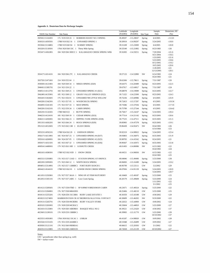
154




SampleDate

Deuterium, δD(‰)

392945115165001 175 N19 E59 24 1 ROBBERS ROOST NO 2 SPRING 39.49597 -115.28047 Spring 6/4/2005 -112.01

393033114593501 178B N19 E62 16 1 UNNAMED SPRING 1 39.50919 -114.99297 Spring 5/24/2005 -118.9

393304115134801 178B N19 E60 04 1 SUMMIT SPRING 39.55108 -115.23000 Spring 6/4/2005 -120.8

393320115130501 178A N20 E60 33C 1 Thirty Mile Spring 39.55549 -115.21892 Spring 8/23/1983 -126

393347114361801 184 N20 E66 30DCC 1 KALAMAZOO CREEK SPRING WR6 39.56383 -114.59251 Spring 7/20/2004 -121.69/21/2004 -118.51/23/2005 -121.65/23/2005 -118.68/12/2005 -119.210/5/2005 -120.611/8/2005 -121

12/13/2005 -120.1

393417114314101 184 N20 E66 27C 1 KALAMAZOO CREEK 39.57133 -114.52890 SW 6/14/1983 -1248/24/1983 -121

393759115471001 154 N20 E55 04 1 39.63306 -115.78611 Spring 7/31/1987 -120

393838114121801 184 N20 E69 34 1 MIKES SPRING (D20) 39.64375 -114.20489 Spring 8/23/2005 -122.5

394045115385701 154 N21 E56 22 1 39.67917 -115.64917 Spring 7/31/1987 -124


394248114135901 185 N21 E68 12 1 GRASS VALLEY SPRINGS (D22) 39.71325 -114.23300 Spring 8/23/2005 -124.3

394320115363601 175 N21 E56 01 1 UNNAMED NR LITTLE WILLOW 39.72236 -115.60986 Spring 6/5/2005 -125.9

394328115342301 175 N21 E57 05 1 WOODCHUCK SPRING 39.72453 -115.57297 Spring 6/5/2005 -119.56

394409115341301 175 N22 E57 33 1 MUD SPRING 39.73586 -115.57036 Spring 6/5/2005 -117.55

394528115162101 175 N22 E59 24 1 CABIN SPRING 39.75789 -115.27244 Spring 6/5/2005 -124.42

394529115143301 178B N60 E22 1 BUTTE SPRING 39.75817 -115.24247 Spring 5/24/2005 -120.4

394623114124101 185 N22 E69 19 1 CEDAR SPRING (D23) 39.77314 -114.21142 Spring 8/23/2005 -120.6

394631114283001 184 N22 E66 23 1 DIPPING TANK SPRING (D28) 39.77525 -114.47511 Spring 8/25/2005 -121.5

395135114282201 184 N23 E66 24 1 ROCK SPRINGS (D29) 39.85983 -114.47278 Spring 8/25/2005 -119.1

395152114552601 179 N23 E62 13B 1 EGAN CREEK 39.86438 -114.92475 SW 8/24/1983 -1266/14/1984 -123

395523114592101 178B N24 E62 29 1 JOHNSON SPRING 39.92319 -114.98922 Spring 5/24/2005 -123.4


395916114260001 184 N24 E67 05 1 UNNAMED SPRING #2 (D25) 39.98783 -114.43342 Spring 8/24/2005 -121


400054114480001 179 N25 E63 18D 1 GOSHUTE CREEK 40.01493 -114.80086 SW 6/15/1983 -1228/24/1983 -124

400243114580301 178B N25 E62 03D 1 SNOW CREEK 40.04521 -114.96836 SW 6/15/1983 -1228/24/1983 -125

400255115293801 176 N25 E57 13AD 1 STATION SPRING AT ORIFICE 40.04846 -115.49490 Spring 5/23/2000 -128

400339115095001 175 N25 E60 12 1 WHITE ROCK SPRING 40.06083 -115.16389 Spring 5/24/2005 -119.2

400405115314901 176 N25 E57 11BBBC1 FORT RUBY RANCH 1 40.06799 -115.53111 GW 5/2/2002 -129

400442114544101 178B N25 E62 01 1 LOWER SNOW CREEK SPRING 40.07836 -114.91139 Spring 5/24/2005 -120.95/24/2005 -120.7

401105115292801 176 N27 E57 36AA 1 NINO SP AT FISH HATCHERY 40.18469 -115.49187 Spring 5/23/2000 -125

401205115301101 176 N27 E57 24DC 1 Cave Creek Spring 40.20179 -115.49608 Spring 5/23/2000 -1241/11/2001 -1225/1/2002 -125

401412115285601 176 N27 E58 07BD 1 SP 0.89MI N BRESSMAN CABIN 40.23671 -115.48324 Spring 5/25/2000 -122

401515115284901 176 N27 E58 06BADD1 40.25406 -115.48110 GW 5/25/2000 -125

401813115255201 176 N28 E58 15CCBB1 RUBY LAKE ESTATES 1 40.30359 -115.43188 GW 4/30/2002 -129

401822115274001 HARRISON PASS CR AT BEDROCK/ALLUVIAL CONTACT 40.30609 -115.46202 SW 9/19/2000 -122

401913115265701 176 N28 E58 09CBDB1 RUBY VALLEY STORE 40.32023 -115.44909 GW 10/8/2002 -124

402010115265001 176 N28 E58 04CBAC1 40.33604 -115.44810 GW 5/25/2000 -127

402343115125801 176 N29 E60 16BDBD1 BASQUE WELL NO 2 40.39521 -115.21620 GW 4/30/2002 -137

402360115190101 176 N29 E59 15BBBC1 40.39983 -115.31770 GW 5/25/2000 -13910/10/2002 -137

402555114591801 178A N30 E62 33CAC 1 USBLM 40.43187 -114.98920 GW 10/9/2002 -128

403334115155101 176 N31 E59 24ABBC1 40.55948 -115.26499 GW 10/9/2002 -127

403958115121101 176 N32 E60 09DBDA1 40.66615 -115.20393 GW 5/1/2002 -122

404335115123801 176 N33 E60 21BDCD1 40.72658 -115.21139 GW 10/10/2002 -127

Notes:GW = groundwater other than spring (e.g. well)SW = surface water

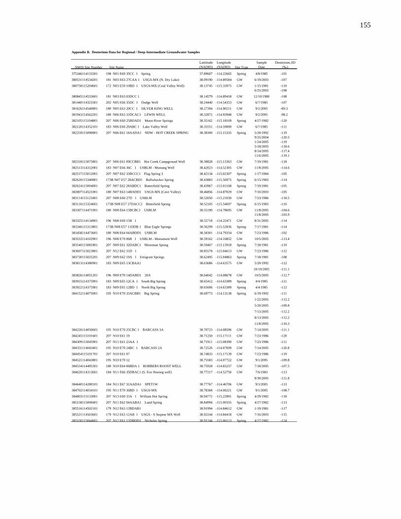
155

Appendix B. Deuterium Data for Regional / Deep-Intermediate Groundwater Samples



SampleDate

Deuterium, δD(‰)

375346114133301 198 N01 E69 35CC 1 Spring 37.89607 -114.22665 Spring 4/8/1985 -101

380531114534201 181 N03 E63 27CAA 1 USGS-MX (N. Dry Lake) 38.09190 -114.89584 GW 6/19/2003 -107

380758115204601 172 N03 E59 10BD 1 USGS-MX (Coal Valley Well) 38.13745 -115.33975 GW 1/15/1981 -1106/25/2003 -108

380845114533601 181 N03 E63 03DCC 1 38.14579 -114.89418 GW 12/10/1980 -108

381440114323301 202 N05 E66 35DC 1 Dodge Well 38.24440 -114.54333 GW 6/7/1985 -107

381626114540801 180 N05 E63 20CC 1 SILVER KING WELL 38.27394 -114.90211 GW 9/2/2005 -89.3

381943114562201 180 N06 E63 31DCAC1 LEWIS WELL 38.32872 -114.93948 GW 9/2/2005 -98.2

382105115104801 207 N06 E60 25BDAD1 Moon River Springs 38.35162 -115.18169 Spring 4/27/1982 -120

382120114352101 183 N06 E66 29ABC 1 Lake Valley Well 38.35551 -114.59000 GW 6/7/1985 -111

382259115090801 207 N06 E61 18AADA1 NDW - HOT CREEK SPRING 38.38300 -115.15335 Spring 5/20/1992 -1199/25/2004 -120.51/24/2005 -1195/18/2005 -118.68/14/2005 -117.411/6/2005 -119.1

382318115075801 207 N06 E61 09CCBB1 Hot Creek Campground Well 38.38828 -115.13363 GW 7/19/1981 -118

382513114312001 183 N07 E66 36C 1 USBLM - Mustang Well 38.42023 -114.52305 GW 11/8/2005 -114.6

382517115012001 207 N07 E62 33BCCC1 Flag Spring 3 38.42134 -115.02307 Spring 1/17/1984 -105

382620115340801 173B N07 E57 28ACBD1 Bullwhacker Spring 38.43883 -115.56975 Spring 6/15/1983 -114

382624115004001 207 N07 E62 28ABDC1 Butterfield Spring 38.43967 -115.01168 Spring 7/19/1981 -105

382807114521001 180 N07 E63 14BADD1 USGS-MX (Cave Valley) 38.46856 -114.87029 GW 7/10/2003 -105

383114115123401 207 N08 E60 27D 1 USBLM 38.52050 -115.21030 GW 7/23/1986 -118.5

383116115324601 173B N08 E57 27DACC2 Bitterfield Spring 38.52105 -115.54697 Spring 6/15/1983 -116

383307114471001 180 N08 E64 15BCBC1 USBLM 38.55190 -114.78695 GW 11/8/2005 -104.611/8/2005 -103.9

383325114134901 196 N08 E69 15B 1 38.55718 -114.22471 GW 8/31/2005 -114

383346115313801 173B N08 E57 11DDB 1 Blue Eagle Springs 38.56299 -115.52836 Spring 7/17/1981 -114

383458114473601 180 N08 E64 04ABDD1 USBLM 38.58301 -114.79334 GW 7/23/1986 -102

383533114102901 196 N08 E70 06B 1 USBLM - Monument Well 38.59162 -114.16832 GW 10/5/2005 -113.4

383540115081801 207 N09 E61 32DABC1 Moorman Spring 38.59467 -115.13918 Spring 7/18/1981 -119

383607115023801 207 N12 E62 31D 1 38.85578 -115.04613 GW 7/23/1986 -112

383730115025201 207 N09 E62 19A 1 Emigrant Springs 38.62495 -115.04863 Spring 7/18/1981 -108

383813114380901 183 N09 E65 13CBAA1 38.63686 -114.63575 GW 5/20/1992 -112

10/19/2005 -111.1

383826114051201 196 N09 E70 14DABD1 20A 38.64042 -114.08678 GW 10/5/2005 -112.7

383915114375901 183 N09 E65 12CA 1 South Big Spring 38.65412 -114.63389 Spring 4/4/1985 -111

383922114375901 183 N09 E65 12BD 1 North Big Spring 38.65606 -114.63389 Spring 4/4/1985 -112

384152114075001 195 N10 E70 33ACBB1 Big Spring 38.69773 -114.13138 Spring 6/19/1992 -111

1/22/2005 -112.2

5/20/2005 -109.8

7/13/2005 -112.2

8/13/2005 -112.2

11/8/2005 -110.3

384226114050601 195 N10 E70 25CBC 1 BARCASS 3A 38.70723 -114.08596 GW 7/14/2005 -111.1

384245115101601 207 N10 E61 19 38.71250 -115.17111 GW 7/23/1986 -120

384309115045901 207 N11 E61 23AA 1 38.71911 -115.08390 GW 7/23/1986 -111

384331114043401 195 N10 E70 24BC 1 BARCASS 2A 38.72526 -114.07699 GW 7/14/2005 -120.8

384454115101701 207 N10 E61 07 38.74833 -115.17139 GW 7/23/1986 -119

384521114043801 195 N10 E70 12 38.75583 -114.07722 GW 9/1/2005 -109.8

384534114495301 180 N10 E64 06BDA 1 ROBBERS ROOST WELL 38.75928 -114.83237 GW 7/18/2005 -107.5

384620114313601 184 N11 E66 35DBAC1 (S. Fox flowing well) 38.77217 -114.52750 GW 7/6/1983 -113

8/30/2005 -111.8

384640114280101 184 N11 E67 32AADA1 SPET1W 38.77767 -114.46706 GW 9/3/2005 -113

384702114034101 195 N11 E70 36BD 1 USGS-MX 38.78384 -114.06221 GW 9/1/2005 -108.7

384803115133001 207 N13 E60 33A 1 William Hot Spring 38.94772 -115.22891 Spring 4/29/1982 -118

385158115000401 207 N11 E62 04AABA1 Lund Spring 38.84994 -115.00335 Spring 4/27/1982 -113

385516114502101 179 N12 E63 12BDAB1 38.91994 -114.84612 GW 1/19/1981 -117

385521114503601 179 N12 E63 12AB 1 USGS - S Steptoe MX Well 38.92244 -114.84418 GW 7/16/2003 -115

385530115044601 207 N12 E61 12DBDD1 Nicholas Spring 38.91244 -115.06113 Spring 4/27/1982 -124

156

Appendix B. Deuterium Data for Regional / Deep-Intermediate Groundwater Samples



SampleDate

Deuterium, δD(‰)

385538115045701 207 N12 E61 02AC 1 Cold Springs - Preston 38.92716 -115.08335 Spring 7/16/1981 -121

6/16/1983 -126

385540115045701 207 N12 E61 02ACAB1 Preston Big Spring 38.93355 -115.08141 Spring 9/25/2004 -122.6

1/24/2005 -122.4

5/21/2005 -120

8/14/2005 -121.2

11/6/2005 -120.4

385546114250501 184 N12 E67 02 1 CEDAR SPRINGS 38.92939 -114.41817 Spring 7/12/2005 -107.4

385613114250401 184 N12 E67 02ACBA1 USBLM (Shoshone pond well) 38.93634 -114.41889 GW 7/6/1983 -109

5/27/1992 -108

1/22/2005 -110.3

5/20/2005 -108.1

7/12/2005 -108.6

8/12/2005 -108.6

11/8/2005 -108.2

390352114305401 184 N14 E66 24BDDD1 USGS-MX (Spring Valley N.) 39.06439 -114.51584 GW 12/12/2005 -83

390457116323401 140A N14 E47 02A 1 Spring 39.08243 -116.54369 Spring 1/1/1974 -128

390541114471301 179 N20 E64 17DD 1 39.09466 -114.78779 GW 6/14/1984 -121

390753116051701 155A N15 E52 35C 1 39.13132 -116.08895 GW 7/31/1987 -119

390754114303001 184 N15 E66 25DCAD1 LAP&W Spring Vly Well 1 39.13161 -114.50917 GW 9/16/1982 -125

390807114282501 184 N15 E67 29 39.13528 -114.47361 GW 6/18/1992 -121

391410116032101 155A N16 E53 30B 1 39.23076 -116.05672 GW 7/31/1987 -123

391637116021801 155A N16 E53 08BCBB1 Fish Creek Springs 39.27687 -116.03922 Spring 7/17/1981 -121

391755115555401 155A N17 E54 31 39.29861 -115.93167 GW 7/31/1987 -118

392411113514301 (C-16-18)22cab-S1 39.40300 -113.86277 Spring 8/26/1981 -109

392527113290901 (C-16-15)13bab-S1 39.42411 -113.48665 Spring 8/25/1981 -111

392731114382801 179 N18 E65 03DA 1 McGill Spring 39.45855 -114.64196 Spring 7/15/1981 -122

392737114021201 (C-15-19)31cbd-S1 39.46014 -114.03763 Spring 5/28/2003 -120

9/24/2004 -119.6

1/22/2005 -120

5/23/2005 -119.4

7/17/2005 -119.7

8/12/2005 -119.8

11/8/2005 -122.8

392815113593001 (C-15-19)31bc -S1 39.47078 -113.99249 Spring 8/26/1981 -121

393212114545001 179 N19 E63 05 1 Spring 39.53660 -114.91475 Spring 7/15/1981 -123

393442114231801 184 N20 E67 26ABBD1 USBLM 39.57633 -114.40029 GW 11/9/2005 -124.3

393946114482301 179 N21 E63 24 1 Spring 39.66271 -114.80724 Spring 1/1/1974 -128

394001114482600 179 N21 E63 24 2 Spring 39.66688 -114.80808 Spring 5/28/1992 -125

394031114465601 179 N21 E64 19BDAD1 39.67521 -114.78308 GW 6/14/1984 -125

394149114302201 184 N21 E66 15DBDD1 WILLOW SPRING 39.69682 -114.50607 Spring 10/20/2005 -122.7

394427115304301 175 N22 E57 25CCCC1 Well at Alligator Ridge 39.74076 -115.51282 GW 4/24/1984 -127

394436115270401 175 N22 E58 28CCCA1 Ram. Res. Wtr Supply Well 39.74326 -115.45198 GW 7/19/1985 -130

394859115363701 154 N23 E56 36DD 1 39.81632 -115.61116 GW 7/31/1987 -122

394949114331802 184 N23 E66 31AB 2 39.83021 -114.55585 GW 7/27/1983 -126

395027113234001 (C-11-14)23dcd-S1 39.84072 -113.39520 Spring 5/29/2003 -111

395029113233601 (C-11-14)23ddc-S1 39.84133 -113.39415 Spring 8/27/1981 -111

395116114451301 179 N23 E64 20AA 1 LAP&W Steptoe Well 1 39.85438 -114.75447 GW 9/16/1982 -124

395226114215401 185 N23 E67 14BA 1 TIPPET SPRING (D24) 39.87383 -114.36585 Spring 8/24/2005 -123.3

395342114532701 179 N23 E63 06 1 Hot Sp, Cherry Creek 39.89493 -114.89169 Spring 1/1/1974 -128

395846113591101 (C-10-19)04ddc-1 39.97944 -113.98639 GW 10/4/2005 -121.6

395935113584601 (C- 9-19)34CCD- 1 39.99299 -113.98000 GW 10/4/2005 -121.7

400119115274801 176 N25 E58 29ABDC2 RV-1 SHALLOW 40.02194 -115.46333 GW 8/20/2002 -121

400119115274802 176 N25 E58 29ABDC3 RV-1 DEEP 40.02194 -115.46333 GW 8/20/2002 -127

9/10/2003 -127

400131115254501 176 N25 E58 27BAAA1 RV-2 40.02528 -115.42917 GW 8/20/2002 -127

8/21/2002 -123

400458114371401 179 N26 E65 34DABA2 40.08271 -114.62141 GW 7/27/1983 -129

400954114442401 179 N27 E64 34DCC 1 40.16493 -114.74086 GW 4/21/1983 -133

6/14/1983 -132

Notes:

GW = groundwater other than spring (e.g. well)

157

Appendix C.

Comparison of Optimization Methods for a Discrete-State Compartment (DSC) Groundwater Accounting Model: Uniform

Random Search (URS), Shuffled-Complex Evolution (SCE), and Multi-Objective Complex Evolution (MOCOM) Algorithms

Kevin Lundmark Graduate Program of Hydrologic Sciences

University of Nevada, Reno

ABSTRACT A discrete-state compartment (DSC) groundwater accounting model for a five-basin area in eastern Nevada was developed for demonstration of the uniform random search (URS) method and shuffled complex evolution (SCE) and multi-objective complex evolution (MOCOM) optimization algorithms. The DSC model is simple, mass balance mixing model which represents hydrographic areas as a series of interconnected cells. Model optimization is achieved by varying the fractional groundwater flows between cells and out of the model domain. A multiple objective optimization problem was posed by evaluating model performance in terms of predicted concentrations and predicted outflows from the model domain. The inclusion of target, minimum outflow rates complicated model optimization, and results suggest that target outflow rates may be better handled by modifications to the accounting model rather than during optimization. The inability of the model to match predicted concentrations to observed concentrations suggest that either concentration data are not representative or a different model is needed.

158

1. INTRODUCTION AND SCOPE This paper presents the results from the optimization of a discrete-state compartment (DSC) groundwater accounting model using a variety of common parameter estimation and uncertainty analysis techniques. The model used for this exercise is a relatively simple mass-balance groundwater accounting model which represents hydrographic basins as a series of connected cells. While simple in its approach, this accounting model provides a useful framework for evaluating combinations of groundwater flow systems and uncertainties associated with predicted groundwater flows.

The groundwater accounting model is described in the section that follows. Because the model includes mass fluxes of an environmental tracer (deuterium) as well as flow rates (volume per unit time), optimization of the model may include aspects dealing with either tracer concentrations or flow rates, and these two variables (concentration and flowrate) may be used to pose an optimization problem involving multiple objective criteria. Multiple-objective optimization problems are characterized by a trade off between objective criteria, and as such, these problems have sets of solutions rather than a single parameter set. The set of solutions which defines the minimum uncertainty in the parameters that can be achieved without assigning subjective relative preference to the objective criteria is referred to as a Pareto set (Yapo et al. 1998).

The scope of this paper is to describe how multiple optimization approaches may be applied to hydrologic model. Optimization approaches applied to the model include the uniform random search (URS) method and the shuffled-complex evolution (SCE) and multi-objective complex evolution (MOCOM) optimization algorithms. The results of the optimization approaches will be presented and discussed with a focus on the tradeoffs between multiple objective criteria based on concentration and outflow predictions from the model.

2. GROUNDWATER ACCOUNTING MODEL

2.1 Water budgets

Water budgets (or water balances) are an application of simple mass conservation equations which may be used to establish the basic hydrologic characteristics of a geographical region (Dingman 2002). The fundamental equation for a water budget is the sum of inputs rates (Q, volume per time) minus the sum of output rates equals the change in storage of the system. If the system is assumed to be at steady-state, then the change in storage is zero and the water budget becomes:

∑ ∑= OutputsInputs QQ

For a groundwater system, inputs may include direct recharge from precipitation, indirect recharge of precipitation from surface water runoff, groundwater inflow from outside the system boundary, or recharge from anthropogenic sources. Groundwater outputs may include discharge as springs, discharge to surface water bodies, evapotranspiration (ET), groundwater outflow to outside the system boundary, and

159

pumping for domestic, agricultural, industrial, and mining uses. Within the Great Basin province in eastern Nevada, the primary contributors of recharge are precipitation and groundwater inflow and that discharge is principally by ET and groundwater outflow, a simplified water budget may be expressed as:

outflowGWETinflowprecip GWDischargeGWRecharge +=+

where recharge from anthropogenic sources and pumping for domestic, agricultural, industrial, and mining uses are assumed to be negligible. This simplified water budget also assumes that groundwater discharged from springs recycles back into the shallow water table where subsequent evaporation or transpiration occurs.

2.2 Groundwater accounting

A groundwater accounting model is a tool which can help verify tabulated water budgets and evaluate interbasin groundwater flows. For a basic mass-balance type groundwater accounting model, simplified mass-balance mixing equations are used to account for inputs and outputs to the system, rather than the standard groundwater flow equation used in typical numerical simulations. The mass-balance model has the same fundamental equation as the water budget; the difference for the mass balance model is that the mass of a substance (or tracer) moving in and out of the system per unit time is used instead of volumes of water.

Considering that the mass flux of a tracer in water may be calculated as its concentration (mass per volume) times the volume of water and assuming this system is at steady state, the mass balance approach may be viewed as a water budget modified to include concentrations, and the general equation may be expressed as:

∑∑==

×=×outin N

jjoutjout

N

iiiniin CQCQ

11)()(

where Qin and Cin represent the flowrate (volume/time) and concentration (mass/volume) for each of Nin inputs and Qout and Cout represent the flowrate and concentration for each of Nout outputs.

The benefit of this approach is that if tracer concentrations vary for different model inputs and between different areas within a system, then modeling the movement of the tracer within the system can provide information on magnitudes and directions of water flow. In this way, groundwater chemistry data are used to help verify the water budget and may provide information on the mixing patterns and source areas for groundwater in the carbonate aquifer system.

2.3 Discrete-State Compartment Model

A groundwater accounting model which has been recently applied to hydrographic basins in eastern Nevada is a modified Discrete-State Compartment (DSC) model. The DSC model is a mixing cell model that represents groundwater systems as a network of interconnected cells. Both water and tracer movements are governed by a set of conservation of mass equations which incorporate water budget (groundwater recharge) and environmental tracer values into iterative water and mass balance

160

calculations for the modeled system. The DSC model is advantageous for use in the Great Basin because it may be applied to systems lacking sufficient information on hydraulic gradients and aquifer parameters necessary to define complex groundwater models (Carroll and Pohll, 2007).

The DSC model was developed by Campana (1975) as a tool to model the mass of any groundwater tracer (ie. groundwater constituents or environmental isotopes) via mixing cell mass-balance equations. Whereas the original DSC model allowed for transient simulations and the use of non-conservative tracers, the DSC model which is applied for this study has been modified to simulate only steady-state conditions of a conservative tracer (Carroll and Pohll, 2007). Consequently, assumptions for cell volumes and source/sink rates are not necessary. Model inputs include the number of cells, rates and concentrations for recharge, and connections between cells. A schematic illustration of a DSC model is shown as Figure 1.

The steady-state assumption requires that volume and mass discharging from a cell is equal to all inputs of volume and mass. The algorithm of an instantaneously mixed cell may be expressed as:

( ) ( )

( ) ( )4342143421

448447648476

rate inflowGW

1,

rate Recharge

1,

inflowGW from Mass

1,

recharge from Mass

1,,

∑∑

∑∑

==

==

+

+= D

k

dkik

N

j

rji

D

k

dk

dkik

N

j

rji

rji

i

QfQ

CQfCQC

where C is a cell’s steady-state modeled concentration. Discharge can occur to another cell (as interbasin groundwater flow within the model domain) or out of the model domain (as ET or interbasin groundwater flow out of the model domain. Therefore,

0.1,1

, =+∑=

outi

P

hhi ff

where P is the number of outflows to adjacent cells from cell i, fi,h is the fraction of flow and mass discharged from cell i and received by cell h, and fi,out is the fraction of flow and mass discharged from cell i out of the model domain.

During model optimization, flow fractions (fi,h and fi,out) and cell ranks are adjusted until the predicted cell concentrations and/or outflows best match observed cell concentrations and/or outflows. The parameters fi,h and fi,out effectively control the volume and mass moving between each cell and out of the model domain. Optimization of the DSC model is achieved by minimizing the error between observed and predicted values for each cell in the model. The process of DSC model optimization has traditionally been performed by manually adjusting cell-to-cell and boundary fluxes until modeled tracer concentrations in each cell most closely match observed values. An example of an objective function for concentration is the weighted root mean squared error for concentration, wRMSE C:

161

where Coi and Cpi are the observed and predicted concentrations in cell i, respectively, N is the number of cells being modeled and iwc is the weight assigned to cell i for the observed concentration.

DSC models have also traditionally not included assumptions relating to discharge of groundwater by ET. In order to incorporate available ET estimates and deter unrealistically low discharge rates, a second objective function was identified based on outflow criteria. Under this scenario, an iteration was penalized if a cell’s outflow rate was less than the estimated groundwater ET rate. In this context, groundwater ET rates represent hypothetical minima for outflow rates from cells in the model. An objective function for targeting these minimum outflow rates is the weighted root mean square error for outflow, wRMSE Out:

where QETi and Qouti are the target (minimum) and predicted outflows for cell i, respectively, N is the number of cells being modeled and wQi is the weight assigned to cell i for the target outflow rate.

3. DISCRETE-STATE COMPARTMENT MODEL OPTIMIZATION

3.1 DSC model application

The study area used for this exercise includes five hydrographic basins in eastern Nevada. These basins are a subset of a larger study area which is the subject of an ongoing groundwater study in White Pine County, Nevada, and adjacent areas in Nevada and Utah. Two hydrographic areas have been subdivided into three sub-basins each. These six sub-basins along with the two undivided hydrographic basins comprise the nine-basin study area for this exercise (Figure 2). Cell connectivity and DSC model inputs for recharge and observed deuterium values for these basins were taken from another report (Lundmark et al., in press). The nine-cell network includes ten cell connections, corresponding to interbasin groundwater flowpaths. These connections plus outflows from five cells yield a DSC model with fifteen optimization parameters. Note that four cells only have one output (outflow from the model domain with no interbasin flow) therefore outflow from these cells are constant (f = 1.0) and are not optimization parameters.

The optimization of the DSC model was accomplished by developing MATLAB controllers which modified input parameters, called the FORTRAN-based DSC model,

( )5.0

1

22

⎟⎟⎟

⎠

⎞

⎜ ⎜ ⎜

⎝

⎛ −

= ∑=

N

CoCpwwRMSE

N

iiiic

C

5 ( )

. 0

1

22

if; 0if;

⎟ ⎟ ⎟

⎠

⎞

⎜ ⎜ ⎜

⎝

⎛

⎭ ⎬ ⎫

⎩⎨⎧

≥

<−

=

∑ =

NQQ

QQQQw

wRMSE

nl

i ETout

EToutioutiETiQ

OUT

162

managed model output, and linked with optimization algorithms. Output from optimization of the DSC example model include interbasin flows (between cells) and outflow from the model domain for each cell, as well as predicted concentrations (deuterium values) for each cell. Optimization results were evaluated to identify the model output associated with Pareto-optimal solutions from each optimization method.

3.2 Uniform random search (URS) optimization

The uniform random search (URS) optimization approach is a technique which relies on brute computational force to evaluate the results from many combinations of parameters. The URS approach involves 1) generation of large sets of parameters using a uniform sampling of the parameter space, 2) model runs with each set of parameter samples and calculation of associated objective measures, and 3) analysis of results in terms of parameter and objective values (Duan et al, 1992). The interpretation of results from the URS analysis may include evaluation of parameter and objective values, or the incorporation of likelihoods or weighting functions in a Bayesian framework.

The URS optimization performed for the DSC included the generation of 5,000 sets of the fifteen optimization parameters using a uniform random number generator. Uniform random distributions were generated between zero and one for each parameter. In order to satisfy the requirement that all outflow fractions for each cell sum to one, random numbers generated for each cell were summed and the fraction used in the DSC model was the random number divided by the sum.

The results from the URS optimization are presented on the plots included as an appendix. These plots show the objective measures wRMSE C and wRMSE Out versus fractional flow parameters for each cell. The plots illustrate that the constraint that all fractions sum to one results in a bias toward lower values for each the parameter sets, with the effect being most pronounced for cell number four.

The objective space plot of the results of the URS optimization of the DSC model (Figure 3) shows the distribution of results’ values for wRMSE C and wRMSE Out. Of the 5,000 parameter sets evaluated, 564 sets resulted in a zero value for wRMSE Out. Of these results, only the point corresponding to the lowest wRMSE C value is considered a Pareto solution (circled). Three other Pareto solutions were identified by the URS approach. The Pareto curve illustrates the tradeoff between the best fit based on concentration (the Pareto solution point furthest to the right) and the fulfillment of the target discharge requirements (Pareto solution point to the left on the y-axis).

Results from the URS method can also be interpreted using a Bayesian Monte Carlo approach, where the results from a URS analysis are assigned a weight based on a likelihood function. In this manner, results from parameter sets with lower errors are given a greater weight that results from parameter sets which gave poor fits. The Monte Carlo analysis performed on the DSC model included a simple likelihood function, the inverse of wRMSE C. Bayesian weights for each of the 5,000 realizations were calculated as the likelihood function of the individual realization divided by the sum of the likelihood functions for all realizations. Model results (e.g. individual interbasin flows and outflows by cell from the model domain) were sorted while maintaining the associated Bayesian weights and the cumulative weights were calculated for each

163

realization. Finally, the 99 % confidence interval for model predictions were calculated as the predicted values associated with cumulative weights of 0.005 and 0.995. The occurrence of 0 values for wRMSE Out prevented the application of the Bayesian Monte Carlo analysis to the URS results using wRMSE Out objective function values.

Figure 4 presents a comparison of interbasin flow and outflow results from the URS analysis. Results include 99% confidence intervals calculated using wRMSE C, the results associated with the parameter set with the lowest wRMSE C, the range of results associated with parameter sets which resulted in wRMSe Out = 0, and the range of values associated with the Pareto set of solutions identified for the URS optimization approach. The results on Figure 4 show that the Bayesian 99% confidence intervals generally have the widest range of values. Relatively wide ranges of values are also associated with results with wMRSE Out values equal to zero. The result associated with the lowest wRMSE C value for interbasin flow between cells four and one is not within the associated 99% confidence intervals, indicating that there are generally similar values for wRMSE C for most realizations. The magnitudes for several Pareto set flows also extend outside the 99% confidence interval ranges (interbasin flows from cells one to three and four to one and outflow from cell three), indicating that relative to the set of ranked, weighted results of the Bayesian analysis, the Pareto set results for these parameters represent relatively extreme outcomes.

3.3 Shuffled complex evolution (SCE) optimization

The shuffled complex evolution (SCE) optimization algorithm is a robust method for identifying global minima to optimization problems. The method includes components of the simplex procedure, controlled random search, competitive evolution, and complex shuffling. The SCE method is described in detail by Duan et al. (1992). A summary of the SCE method is as follows: 1) a set of sample points are generated in the feasible parameter space, 2) objective function values are evaluated for each point and each point is ranked by their objective value, 3) the points are divided into complexes and each complex evolves within objective space, 4) evolved complexes exchange (shuffle) and the process is repeated until the samples converge to a specified tolerance or until a maximum number of iterations has been performed.

The SCE method is a single objective optimization method, so for models which include multiple objective criteria, such as the DSC model example, the objective functions are typically combined using weighting factors. The SCE optimization which was performed for the DSC model included the variation of weights for the wRMSE C (XC) and wRMSE Out (XO) where XC + XO = 1. The weight XO was varied from 0 to 1 by 0.1 increments, resulting in a set of eleven separate SCE runs and eleven optimal parameter sets (Figure 4). The plot of SCE solutions in parameter space shows that whenever the weight for wRMSE Out was >0, the SCE algorithm found a solution satisfying conditions to generate a wRMSE Out = 0, plotted on the y-axis of Figure 5. Of the ten solutions with wRMSE Out =0, only the solution with the lowest value of wRMSE C is considered to be a Pareto solution; this point corresponds to a wRMSE Out weight of XO = 0.5. The other Pareto solution resulted from no contribution of wRMSE

164

Out to the objective function (XO = 0) and represents the global minimum based on concentration.

3.4 Multi-objective complex evolution (MOCOM) optimization

The multi-objective complex evolution (MOCOM) optimization method is a general optimization algorithm which was designed for use with models with multiple possible objective criteria. The MOCOM algorithm is described by Yapo et al. (1998) as an extension of the SCE optimization algorithm which combines the strengths of controlled random search, competitive evolution, Pareto ranking, and a multi-objective downhill simplex search. The MOCOM method includes similar aspects as SCE, most notably complex evolution in objective space; however, the MOCOM algorithm does not include exchange (shuffling) between different complexes. The output from optimization by MOCOM is the generation of a Pareto curve of a user-specified number of points.

Application of the MOCOM approach to the example DSC model was complicated by the wRMSE Out objective function. In general, the MOCOM approach resulted in a Pareto curve or a single solution depending on the initial sample population and whether the samples converged to the line decried by wRMSE Out = 0. An example of output from MOCOM when a Pareto curve was found is shown in Figure 6. The Pareto curve includes one sample (at far left) with a wRMSE Out = 0 and the rest of samples with wRMSE Out > 0 and with wRMSE C values which are less than the wRMSE C value associated with the sample at wRMSE Out = 0. The series of plots shown in Figure 7 illustrate an example of a MOCOM optimization in which the sample points converge to a single value. The convergence progresses from an early state where multiple points identify the wRMSE Out = 0 minimum, followed by the convergence of all sample points to the wRMSE Out = 0 line, and concluding when all samples converge to a single point.

Twenty samples were used for the MOCOM simulations described above and shown in Figures 5 and 6. MOCOM simulations were run with greater than twenty points, however these trials were observed to result in convergence of all points to the wRMSE Out = 0 line followed by a period of very slow convergence of samples toward a reduced number of points.

4. SUMMARY AND DISCUSSION

A comparison of results from the Pareto solution sets from each optimization approach is shown for flows in Figure 8. The flows which result from the Pareto set of the URS optimization generally displays the widest range. Ranges associated with the SCE Pareto set were also relatively large. The difference between the 20-point MOCOM Pareto set and the single-point MOCOM solution is quite large for some flows, indicating that the results for optimization of the DSC model by this method are strongly dependent on the initial population of sample points and whether these points converge to the objective-space line associated with wRMSE Out = 0. Results from the SCE optimization approach appear most useful because of their clear demonstration of the effects of subjective weights of objective functions on model predictions.

165

Outflow results from the Pareto solution sets from each optimization method were close to greater than the target (minimum) groundwater ET outflows; however, with the exception of the single-point MOCOM solutions, each optimization approach resulted in a Pareto solution for at least one cell where the outflow was less than the target (minimum) groundwater ET rate. This illustrates the effect of the concentration objective function (wRMSE C) on the solution set.

The ranges of observed concentrations for each cell associated with the Pareto solutions for each optimization approach are shown in Figure 9. Cells four, six, and eight are upgradient (i.e. not downgradient of any other cells); this is apparent in their constant observed concentrations. For these cells, the observed concentrations are always equal to the concentration of recharge. The remaining, downgradient-type cells displayed a relatively low degree of variability in the ranges of observed concentrations associated with the Pareto sets, and with the exception of cell three, no downgradient cell achieved a predicted concentration equal to the observed concentration. The inability for either upgradient or downgradient cells to match the observed concentrations indicates that either 1) a different or more elaborate model is needed to achieve a better match, 2) the recharge and/or observed concentrations are not representative of actual conditions, or 3) some combination of 1) and 2).

The results from the optimization of the DSC model using URS, SCE, and MOCOM optimization approaches indicate that model optimization was complicated by the outflow objective function, wRMSE Out, which could have a value of zero for many combinations of parameters. The application of the current DSC to groundwater accounting problems which include target (minimum) groundwater ET discharge rates is limited in that the current model does not allow for the input of these target rates as boundary conditions. Optimization of this type of groundwater accounting problem may be better handled by either a more complicated model or a revised DSC model which includes fixed discharge rates.

Acknowledgement This work was originally prepared for the course GEOL701s - Parameter Estimation and Uncertainty Analysis. The approach and discussion were heavily influenced by the course material and through interaction with the course’s instructor, Dr. Doug Boyle.

5. REFERENCES Campana, M. E. Finite-state models of transport phenomena in hydrologic systems, Ph.D.

Dissertation, University of Arizona, Tuscon, 1975.

Carroll, R.W.H. and G. M. Pohll. draft. A user's manual for the Discrete-state Compartment Model - Shuffled Complex Evolution (DSCM-SCE). Division of Hydrologic Sciences Publication. Desert Research Institute

Dingman, S.L. 2002. Physical Hydrology. Prentice-Hall, Inc. Upper Saddle River, New Jersey. 2nd ed.

166

Duan, Q., Gupta, V.K., Sorooshian, S., 1992. Effective and efficient global optimization for conceptual rainfall-runoff models. Water Resources Research 28(4): 1015-1031.

Lundmark, K.W., G.M. Pohll and R.W.H. Carroll. draft. Steady State Water Budget Accounting Model for Water Resources of the Basin and Range Carbonate Aquifer System in White Pine County, Nevada, and Adjacent Areas in Nevada and Utah. Division of Hydrologic Sciences Publication No. 412XX. Desert Research Institute.

Yapo, P.O., Gupta, H.V., Sorooshian, S. 1998. Multi-objective global optimization for hydrologic models. Journal of Hydrology 204 (1998) 83-97

167

Figure 1. DSC Model Components

Figure 2. DSC Model Application

168

Figure 3. Results from URS optimization, shown in objective space with Pareto solutions circled

169

Figure 4. Comparison of results from URS optimization, including 99% Bayesian confidence intervals using wRMSE C, best objective criteria results for wRMSE C and wRMSE Out, and Pareto solutions

170

Figure 5. Results from SCE optimization, shown in objective space with Pareto solutions circled

Xo = 0Xo = 0.1

Xo = 0.2Xo = 0.3

Xo = 0.4

Xo = 0.5

Xo = 0.6

Xo = 0.7

Xo = 0.8Xo = 0.9

Xo = 1

0.8

0.9

1

1.1

1.2

1.3

1.4

0 0.5 1 1.5 2 2.5 3

wRMSE Out

wR

MSE

C

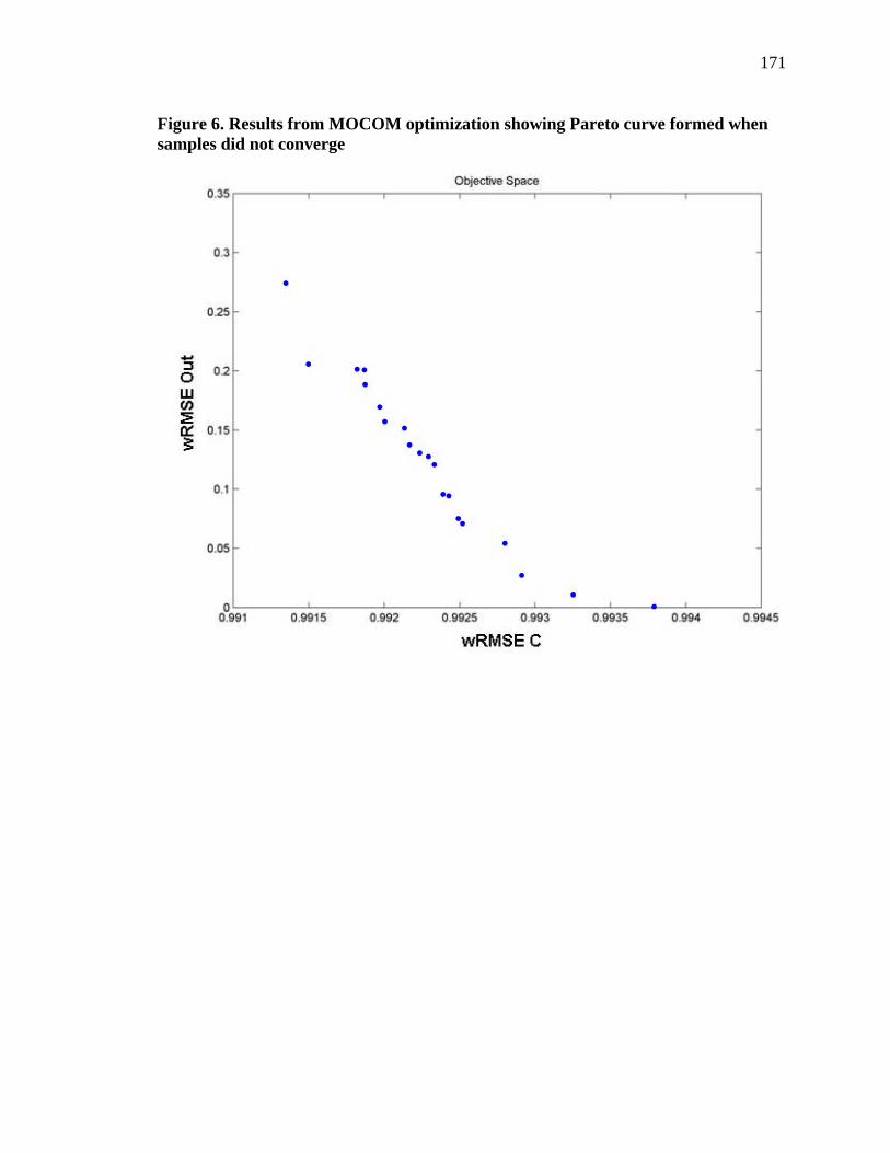
171

Figure 6. Results from MOCOM optimization showing Pareto curve formed when samples did not converge

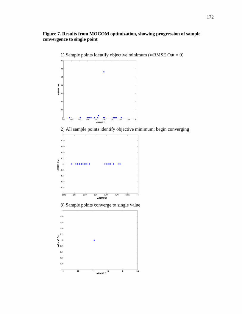
172

Figure 7. Results from MOCOM optimization, showing progression of sample convergence to single point

1) Sample points identify objective minimum (wRMSE Out = 0)

2) All sample points identify objective minimum; begin converging

3) Sample points converge to single value

173

Figure 8. Results from all optimization approaches, shown as ranges of flows predicted by DSC model for Pareto optimal solutions

174

Figure 9. Results from all optimization approaches, shown as ranges of deuterium values predicted by DSC model for Pareto optimal solutions

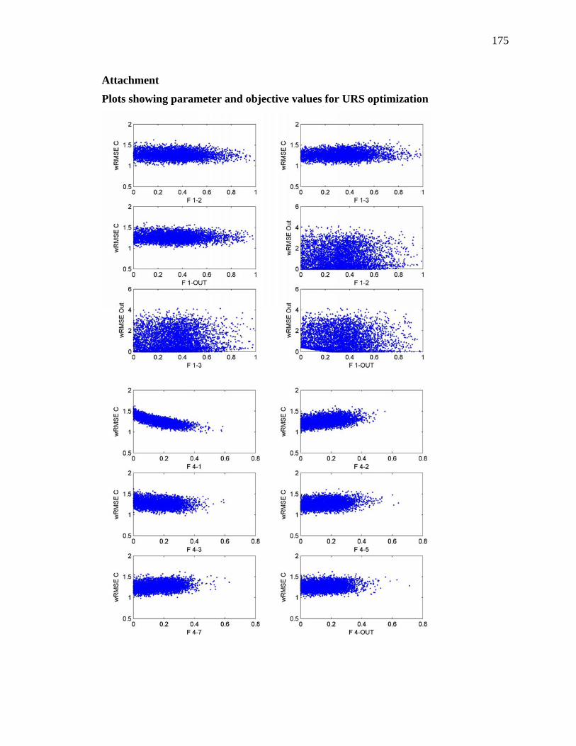
175

Attachment

Plots showing parameter and objective values for URS optimization

176

Attachment


177

Attachment


regional water budget accounting and uncertainty … water budget accounting and uncertainty...

Documents