Regression and Causation: A Critical Examination ofSix Econometrics Textbooks

Bryant Chen and Judea PearlUniversity of California, Los Angeles

Computer Science DepartmentLos Angeles, CA, 90095-1596, USA

(310) 825-3243

September 10, 2013

Abstract

This report surveys six influential econometric textbooks in terms of their math-ematical treatment of causal concepts. It highlights conceptual and notational differ-ences among the authors and points to areas where they deviate significantly frommodern standards of causal analysis. We find that econonometric textbooks vary fromcomplete denial to partial acceptance of the causal content of econometric equationsand, uniformly, fail to provide coherent mathematical notation that distinguishes causalfrom statistical concepts. This survey also provides a panoramic view of the state ofcausal thinking in econometric education which, to the best of our knowledge, has notbeen surveyed before.

1 Introduction

The traditional and most popular formal language used in econometrics is the structuralequation model (SEM). While SEMs are not the only type of econometric model, they arethe primary subject of each introductory econometrics textbook that we have encountered.An example of an SEM taken from (Stock and Watson, 2011, p. 3) is modeling the effect ofcigarette taxes on smoking. In this case, smoking, Y , is the dependent variable, and cigarettetaxes, X, is the independent variable. Assuming that the relationship between the variablesis linear, the structural equation is written Y = βX + ε. Additionally, if X is statisticallyindependent of ε, often called exogeneity, linear regression can be used to estimate the valueof β, the “effect coefficient”.

More formally, an SEM consists of one or more structural equations, generally writtenas Y = X

′β + ε in the linear case, in which Y is considered to be the dependent or effect

variable, X =< X1, X2, ..., Xn > a vector of independent variables that cause Y , andβ =< β1, β2, ..., βn > a vector of slope parameters such that x

′β is the expected value of

Y given that we intervene and set the value of X to x. Lastly, ε is an error term that

1

Real-World Economics Review, Issue No. 65, 2-20, 2013.

TECHNICAL REPORT R-395

September 2013

represents all other direct causes of Y , accounting for the difference between X′β and the

actual values of Y 1. If the assumptions underlying the model are correct, the model is capableof answering all causally related queries, including questions of prospective and introspectivecounterfactuals2. For purposes of discussion, we will use the simplest case in which thereis only one structural equation and one independent variable and refer to the structuralequation as Y = βX + ε.

The foundations for structural equation modeling in economics were laid by Haavelmo inhis paper, “The statistical implications of a system of simultaneous equations” (Haavelmo,1943). To Haavelmo, the econometric model represented a series of hypothetical experi-ments. In his 1944 paper, “The Probabilistic Approach in Econometrics”, he writes:

“What makes a piece of mathematical economics not only mathematics but also eco-nomics is, I believe, this: When we have set up a system of theoretical relationships anduse economic names for the otherwise purely theoretical variables involved, we have in mindsome actual experiment, or some design of an experiment, which we could at least imaginearranging, in order to measure those quantities in real economic life that we think mightobey the laws imposed on their theoretical namesakes” (Haavelmo, 1944, p. 5).

Using a pair of non-recursive equations with randomized ε’s, Haavelmo shows that βxin the equation y = βx + ε is not equal to the conditional expectation, E[Y |x], but ratherto the expected value of Y given that we intervene and set the value of X to x. This“intervention-based expectation” was later given the notation E[Y |do(x)]in (Pearl, 1995)3.

In the years following Haavelmo’s 1944 paper, this interpretation has been questionedand misunderstood by many statisticians. When Arthur Goldberger explained that βx maybe interpreted as the expected value of Y “if x were fixed,” Nanny Wermuth replied thatsince βx 6= E[Y |x], “the parameters... cannot have the meaning Arthur Golberger claims”(Goldberger, 1992; Wermuth, 1992).

(Pearl, 2012b) summarizes the debate in the following way: For statisticians like Wer-muth, structural coefficients have dubious meaning because they cannot be expressed in thelanguage of statistics, while for economists like Goldberger, statistics has dubious substanceif it excludes from its province all aspects of the data generating mechanism that do notshow up in the joint probability distribution.

Econometric textbooks fall on all sides of this debate. Some explicitly ascribe causalmeaning to the structural equation while others insist that it is nothing more than a com-

1A more precise definition of the SEM invokes counterfactuals and reads X′β + ε = Yx(u), where Yx(u)

is the counterfactual “the value that Y would take in unit u, had X been x” (see Simon and Rescher 1966,Balke and Pearl 1995, Heckman 2000, Pearl 2012b, and Appendix A).

2Prospective counterfactual queries are queries of the form, “What value would Y take if X were set tox?” Introspective counterfactual queries are queries of the form, “What would have been the value of Y ifX had been set to x?”

3The expression E[Y |do(x)] can also be interpreted as the expected value of Y in an ideal randomizedexperiment for a subject assigned treatment X = x. Clearly, E[Y |do(x)] does not necessarily equal E[Y |x].For example, the expected performance of an employee at an earning bracket of X = x is different fromthe expected performance if management decides to set someone’s earning to X = x. A simple recipe forcomputing E[Y |do(x)] for a given model is provided in Appendix A, which provides formal definitions ofcounterfactuals and their relations to structural equations and the do(x) operator.

2

pact representation of the joint probability distribution. Many fall somewhere in the middle–attempting to provide the econometric model with sufficient power to answer economic prob-lems but hesitant to anger traditional statisticians with claims of causal meaning. The endresult for many textbooks is that the meaning of the econometric model and its parametersare vague and at times contradictory.

We believe that the source of confusion surrounding econometric models stems from thelack of a precise mathematical language to express causal concepts. In the 1990s, progress ingraphical models and the logic of counterfactuals led to the development of such a language(Pearl, 2000). Significant advances in causal analysis followed. For example, algorithms forthe discovery of causal structure from purely observational data were developed (Verma andPearl, 1990; Spirtes et al., 1993; Verma, 1993) and the problem of causal effect identifiabilitywas effectively solved for non-parametric models (Pearl, 1995; Tian and Pearl, 2002; Huangand Valtorta, 2006; Shpitser and Pearl, 2006; Shpitser, 2008). These and other advanceshave had marked influence on several research communities (Glymour and Greenland, 2008;Morgan and Winship, 2007) including econometrics (Heckman, 2008; White and Chalak,2009), but their benefits are still not fully utilized (Pearl, 2012b).The purpose of this reportis to examine the extent to which these and other advances in causal modeling have benefitededucation in econometrics. Remarkably, we find that not only have they failed to penetratethe field but even basic causal concepts lack precise definitions and, as a result, continue tobe confused with their statistical counterparts.

In this paper, we survey six econometrics textbooks in order to analyze their interpreta-tion and usage of the econometric model and compare them to modern standards of causalanalysis.

2 Criteria for Evaluation

In evaluating textbooks, we ask the following questions: What does the author believe isthe purpose of an econometric model? To which problems can it be applied? How doesthe author interpret the model parameters and the structural equation? Does the authorconsider βx to be equal to the expected value of Y given x, E[Y |x], or the expected valueof Y given that we intervene and set X to x, E[Y |do(x)]? Does the author make clear theassumptions necessary to answer the problems that econometrics is expected to solve?

To answer these questions, we formulated 11 evaluation criteria and grouped them underthree categories. We also state the “ideal”4 answers to these questions.

Applicability of Econometric Models

1. Does the author present example problems that require causal reasoning?

2. Does the author present example problems that require prediction alone?

A predictive problem is one of the form, “Given that we observe X to be x, what value canwe expect Y to take?” Many econometrics textbooks begin with example problems that they

4By ”ideal” we mean consistent with modern analysis, as expressed in articles dealing specifically withthe causal interpretation of structural equation models (Heckman, 2008; Leamer, 2010; Nevo and Whinston,2010; Keane, 2010; Pearl, 2012a).

3

expect econometric methods to solve. We use these examples to determine the author’s viewon the purpose and applicability of the econometric model. Since both predictive and causalproblems are of interest to economists, both should be exemplified in econometrics textbooks.

Interpreting Model Parameters

3. Does the author state that each structural equation in the econometric model is meantto convey a causal relationship?

4. Does the author define β by the equality, βX = E[Y |X]?

Clearly, since the structural equation represents a causal relationship between X andY , it is incorrect to define β by βX = E[Y |X], though the equality may occasionally besatisfied.

5. Does the author define the error term as being the difference between E[Y |X] and Y ?

6. Does the author interpret the error term as omitted variables that (together with X)determine Y ?

7. Does the author state that each structural equation in the econometric model is meantto capture a ceteris paribus or “everything else held fixed” relationship?

The notion of ceteris paribus is sometimes used by economists and is closely tied to directcausation. If we hold all other variables fixed then any measured relationship between Xand Y must be causal. When we write Y = βX+ε, where ε represents all other direct causesof Y , then β must capture a ceteris paribus and, therefore, causal relationship between Xand Y . It is for this reason that we examined whether the author explicitly states that thestructural equation captures a ceteris paribus relationship.

8. Does the author assume that exogeneity of X is inherent to the model?

Economists consider X to be exogenous in the equation Y = βX + ε if X is independent ofε, where ε represents all factors that have influence on Y when X is fixed5. An example ofexogeneity is an ideal randomized experiment. Subjects are randomly assigned to a treatmentor control group, ensuring that X is distributed independently of all personal characteristicsof the subject. As a result, X and ε are independent and X is exogenous. Clearly, if X isexogenous β can be estimated using linear regression.

However, if βX is incorrectly interpreted as E[Y |X] and ε incorrectly defined as Y −E[Y |X] (as is done in the text by Hill, Griffiths, and Lim) then ε will always be uncorrelatedwith X and the statement that X is uncorrelated with ε is vacuous.

Moreover, if all we care about is the conditional expectation then it does not matterwhether confounders or other causal biases are present, as regression will allow proper es-timation of the slope of the equation E[Y |X] = αX so long as the relationship between X

5From a causal analytic perspective, X is exogeneous if E[Y |X] = E[Y |do(X) (Pearl, 2000). However, forpurposes of this paper, we will use the aforementioned definition in which X is exogenous if it is independentof ε. Note that if X is independent of ε then E[Y |X] = E[Y |do(X)]. The converse may not hold. Forexample, when ε is a vector of factors with cancelling influences on Y .

4

and E[Y |X] is linear. In contrast, forcing X to be exogenous (e.g. through a randomized ex-periment) will estimate the interventional expectation and not the conditional expectation,which are not necessarily equal.

While exogeneity allows for unbiased estimation of β, it should not be considered animplicit assumption of the model. β retains its causal interpretation as β = δ

δXE[Y |do(X)]

regardless of whether X and ε are correlated or not. Moreover, exogeneity is a sufficientbut not a necessary condition for identification. By requiring that exogeneity be a defaultassumption of the model, we limit its application to trivial and uninteresting problems, pro-viding no motivation to tackle more realistic problems (say, through the use of instrumentalvariables).

Distinguishing E[Y |X] and E[Y |do(X)]

9. Does the author make clear the difference in the assumptions needed for answeringcausal as opposed to predictive problems?

10. Does the author use separate notation for E[Y |do(X)] and E[Y |X]?

11. Does the author use separate notation for the slope of the line associated with E[Y |X]and that associated with E[Y |do(X)]?

Many books present both predictive and interventional problems as applications for econo-metric analysis. Not all of them discuss the distinction between them despite the fact thatthey require fundamentally different assumptions and, at times, a different methodology. Atthe core of this distinction is whether the model is meant to estimate E[Y |X] or E[Y |do(X)].Clearly, if βX = E[Y |do(X)] is estimated (as opposed to E[Y |X]) when attempting to makepredictions, the answer may be drastically wrong. Utilizing explicit notation for the inter-ventional distributions is essential for avoiding such errors.

Remarkably, all of the econometrics textbooks surveyed refer to the structural equationas the “regression” equation. This is another source of confusion because “regression” isused to refer to the best-fit line. Using the same term to refer to both the structural andbest-fit lines further increases the confusion between interventions and predictions.

3 Results

We surveyed the following textbooks:

• Greene, W. Econometric Analysis. Pearson Education, New Jersey. 7th edition, 2012.

• Hill, R., Griffiths, W., and Lim, G. Principles of Econometrics. John Wiley & SonsInc. New York. 4th edition, 2011.

• Kennedy, P. A Guide to Econometrics. Blackwell Publishers, Oxford. 6th edition,2008.

• Ruud, P. An Introduction to Classical Econometric Theory. Oxford University Press,Oxford. 1st edition, 2000.

5

• Stock, J.; Watson, M. Introduction to Econometrics. Pearson Education, Massachusetts.3rd edition, 2011.

• Wooldridge. Introductory Econometrics: A Modern Approach. South-Western CollegePub. 4th edition, 2009.

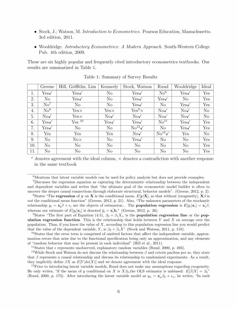
These are six highly popular and frequently cited introductory econometrics textbooks. Ourresults are summarized in Table 1.

Table 1: Summary of Survey Results

Greene Hill, Griffiths, Lim Kennedy Stock, Watson Ruud Wooldridge Ideal

1. YesX YesX No YesX No6 YesX Yes2. No YesX No YesX YesX No Yes3. No7 No No YesX No YesX Yes4. No8 Yes× Yes× Yes9× NoX NoX No5. NoX Yes× NoX NoX NoX NoX No6. YesX Yes 10 YesX YesX No11 YesX Yes7. YesX No No No12X No YesX Yes8. Yes Yes Yes NoX No13X Yes No9. No No× No YesX No No Yes10. No No No No No No Yes11. No No No No No No YesX denotes agreement with the ideal column, × denotes a contradiction with another response

in the same textbook

6Mentions that latent variable models can be used for policy analysis but does not provide examples.7Discusses the regression equation as capturing the deterministic relationship between the independent

and dependent variables and writes that “the ultimate goal of the econometric model builder is often touncover the deeper causal connections through elaborate structural, behavior models”. (Greene, 2012, p. 2).

8States “The regression of y on X is the conditional mean, E[y|X], so that without [exogeneity], Xβ isnot the conditional mean function” (Greene, 2012, p. 21). Also, “The unknown parameters of the stochasticrelationship yi = x

′

iβ + εi are the objects of estimation... The population regression is E[yi|xi] = x′

iβ,

whereas our estimate of E[yi|xi] is denoted yi = x′

ib.” (Greene, 2012, p. 26).9States “The first part of Equation (4.5), β0 + β1Xi, is the population regression line or the pop-

ulation regression function. This is the relationship that holds between Y and X on average over thepopulation. Thus, if you knew the value of X, according to this population regression line you would predictthat the value of the dependent variable, Y , is β0 + β1X” (Stock and Watson, 2011, p. 110).

10States that the error term is comprised of omitted factors that affect the independent variable, approx-imation errors that arise due to the functional specification being only an approximation, and any elementsof “random behavior that may be present in each individual” (Hill et al., 2011).

11States that ε represents unobserved, explanatory random variables (Ruud, 2000, p. 493).12While Stock and Watson do not discuss the relationship between β and ceteris paribus per se, they state

that β represents a causal relationship and discuss its relationship to randomized experiments. As a result,they implicitly define βX as E[Y |do(X)] and we denote agreement with the ideal response.

13Prior to introducing latent variable models, Ruud does not make any assumptions regarding exogeneity.He only writes, “if the mean of y conditional on X is Xβ0,the OLS estimator is unbiased: E[β|X] = β0”(Ruud, 2000, p. 173). After introducing the latent variable model as yn = x

′

nβ0 + εn, he writes, “In each

6

3.1 Greene (2012)

Greene writes, “The ultimate goal of the econometric model builder is often to uncover thedeeper causal connections through elaborate structural, behavior models” (Greene, 2012, pp.5-6). Consistent with this goal, Greene provides seven applications of econometric modelingas examples (ibid., p. 3), each of which requires the estimation of causal effects. Amongthem are the effect of different policies on the economy, the effect of a voluntary trainingprogram in work environments, the effect of attending an elite college on future income, andthe effect of smaller class sizes on student performance.

Although Greene acknowledges the goal of economic modeling to be the establishment orestimation of “causal connections”, he does not explicitly discuss the role of model param-eters in pursuing this goal and refrains from attributing causal interpetation to β. Instead,he relates econometric models to the conditional expectation, writing, “The model builder,thinking in terms of features of the conditional distribution, often gravitates to the expectedvalue, focusing attention on E[y|x]...” (ibid., p. 12). At the same time, Greene also suggeststhat β carries meaning beyond that of the conditional expectation, writing, “The regres-sion of y on X is the conditional mean, E[y|X], so that without [exogeneity], Xβ is notthe conditional mean function” (ibid., p. 21). He does not, however, tell readers what βstands for, what it is used for, or why it justifies all the attention given to it in the book.Instead, he writes, “For modeling purposes, it will often prove useful to think in terms of‘autonomous variation.’ One can conceive of movement of the independent variables outsidethe relationship defined by the model while movement of the dependent variable is consideredin response to some independent or exogenous stimulus” (ibid., p. 13). While this may be alegitimate way of thinking about causal effects, depriving “β” of its causal label creates theimpression that economic models incorporate ill-defined parameters that require constantre-thinking to ascertain their interpretation14.

Later, when discussing endogeneity and instrumental variables, Greene seems to suggestthat a natural experiment and instrumental variable is needed to bestow causal meaningto β. He writes, “The technique of instrumental variables estimation has evolved as amechanism for disentangling causal influences... when the instrument is an outcome of a‘natural experiment,’ true exogeneity is claimed... On the basis of a natural experiment,the authors identify a cause-and-effect relationship that would have been viewed as beyondthe reach of regression modeling under earlier paradigms” (ibid., p. 252). Here the readerwonders why the coefficient β, considered under endogeneity, would not deserve the title“cause and effect relationship” unless a good instrument is discovered by imaginative authors.

Up to this point, Greene has made only passing references to the relationship betweenstructural parameters (e.g., β), regression, and causality. In section 19.6, “Evaluating Treat-ment Effects”, however, Greene introduces potential outcomes and discusses causal effectsexplicitly (ibid., p. 889); gone are the hesitation and ambiguities that marred the discussion

model that we describe, at least one of the explanatory variables in xn is correlated with εn so that E[εn|xn]is a function of xn and, therefore, not zero. This in turn implies that E[yn|xn] 6= x

′

nβ0 and that the OLS fitof ynto xn will yield inconsistent estimates of β0” (Ruud, 2000, p. 491).

14In a personal correspondence (2012), Greene wrote, “The precise definition of effect of what on what issubject to interpretation and some ambiguity depending on the setting. I find that model coefficients areusually not the answer I seek, but instead are part of the correct answer. I’m not sure how to answer yourquery about exactly, precisely carved in stone, what β should be.”

7

of structural equations. Here, Rubin’s notation for counterfactuals is introduced and Greenediscusses the estimation of causal effects using regression, propensity score matching, andregression discontinuity (instrumental variables are mentioned in an earlier chapter). How-ever, Greene provides no connections between treatment effects defined in this chapter andthe structural equations that were the subject of discussion in the 18 earlier chapters. Theimpression is, in fact, created that the previous chapters were a waste of time for researchersaiming to estimate causal effects, which the book defines as, “The ultimate goal of theeconometric model builder”.

In section 19.6.1, “Regression Analysis of Treatment Effects”, Greene presents the equa-tion, earningsi = x

′

iβ + δCi + εi and asks, “Does δ measure the value of a college education(assuming that the rest of the regression model is correctly specified)? The answer is noif the typical individual who chooses to go to college would have relatively high earningswhether or not he or she went to college...” The answer is, in fact, YES15. The only wayto interpret Greene’s negative answer is to assume that the equation is regressional andthat δ is simply the slope of the regression line. However, as mentioned above, Greene alsosuggests that “regression” parameters (ibid., p. 21) are more than just slopes of regressionlines. Indeed, this is the interpretation that is generally used throughout the textbook. Thisinconsistency is a major source of confusion to students attempting to understand the mean-ing of parameters like “β” or “δ”. In summary, while Greene provides the most detailedaccount of potential outcomes and counterfactuals of all the authors surveyed, his failure toacknowledge the oneness of the potential outcomes and structural equation frameworks islikely to cause more confusion than clarity, especially in view of the current debate betweentwo antagonistic and narrowly focused schools of econometric research (See Pearl 2009, p.379-380).

3.2 Hill, Griffiths, and Lim (2011)

In the first chapter of the text by Hill, Griffiths, and Lim, the authors discuss the role ofeconometrics in aiding both prediction and policy making. On pp. 3-4, they present severalproblems as examples, some of which are causal and some of which are predictive:

• “A city council ponders the question of how much violent crime will be reduced if anadditional million dollars is spent putting uniformed police on the street.

• “The owner of a local Pizza Hut must decide how much advertising space to purchasein the local newspaper, and thus must estimate the relationship between advertisingand sales.

• “You must decide how much of your savings will go into a stock fund, and how muchinto a money market. This requires you to make predictions of the level of economicactivity, the rate of inflation, and interest rates over your planning horizon (Hill et al.,2011)”.

15δ, in this structural equation, measures precisely the value of a college education, regardless of whatsort of individuals choose to go to college. While the OLS estimation of δ will be biased, the meaning of δremains none other but the “value of college education”.

8

However, in explaining the meaning and usage of the econometric model, the text makesno mention of causal vocabulary and instead relies on statistical notions like conditionalexpectation. For example, on p. 43, they write, “the economic model summarizes what theorytells us about the relationship between [x] and the... E(y|x)” and the “simple regressionfunction” of the model is defined as E(y|x) = β1 + β2x (ibid., pp. 43) where β1 is defined as

E(y|x = 0) and β2 as dE(y|x)dx

. At no point is causality or ceteris paribus mentioned.This interpretation leaves the econometric model unable to guide policy making and solve

the aforementioned problems requiring causal inference. Indeed, these problems seem to beforgotten in chapter 2 when the econometric model is introduced and instead, we find onlypredictive examples: “An econometric analysis of the expenditure relationship can provideanswers to some important questions, such as: If weekly income goes up by $20, how muchwill average weekly food expenditure rise? Or, could weekly food expenditures fall as incomerises? How much would we predict the weekly expenditure on food to be for a householdwith an income of $800 per week?” (ibid., p. 44).

At the same time, when discussing the assumptions inherent to the econometric modelthe text states that “the variable x is not random” (ibid., p. 45) and explains this assumptionusing an example of a McDonald’s owner “[setting] the price (x) and then [observing] thenumber of Big Macs sold (y) during the week. The following week the price could be changed,and again the data on sales collected.” (ibid., p. 46 - 47). Clearly, requiring that the databe generated by a process in which X is fixed by intervention suggests that β1 + β2x hasmeaning beyond that of the E(y|x).

Later, the authors introduce the error term as e = y − E(y|x) (ibid., p. 46) and theregression equation is defined as y = β1 + β2x + e. Using these definitions, they relax theassumption that x be “fixed” explaining that it is unnecessary so long as it is uncorrelatedwith the error term (ibid., p. 402). Not only is the requirement that ε be uncorrelated withX redundant when e is defined as the residual, y−E(y|x), but relating it to the assumptionthat x is “not random” leaves readers in a state of total confusion regarding the meaning ofβ.

3.3 Kennedy (2008)

Kennedy introduces the structural model using an example where consumption, C, is thedependent variable, and income Y is the independent variable. He writes the structuralequation as C = f(Y ) + ε or C = β1 + β2Y + ε in the linear case, where ε is a distur-bance term, and adds, “Without the disturbance term the relationship is said to be exactor deterministic...” (Kennedy, 2008, p. 3). Kennedy then writes that “some econometri-cians prefer to define the relationship between C and Y discussed earlier as ‘the mean ofC conditional on Y is f(Y ),’ written as E(C|Y ) = f(Y ).” This [says Kennedy] “spells outmore explicitly what econometricians have in mind when using this specification” (ibid., p.9). This unfortunately is wrong; the conditional interpretation E(C|Y ) = f(Y ) is preciselywhat econometricians do not have in mind in writing the structural equation C = f(Y ) + ε.Both Haavelmo (1943) and Goldberger (1992) have warned econometricians of the pitfallslurking in this interpretation. Oddly, Kennedy is well aware of the difference between thetwo interpretations and writes: “The conditional expectation interpretation can cause someconfusion” (ibid.), yet he fails to tell readers which of the two interpretations they should

9

adopt and why the conditional interpretation does not capture “what econometricians havein mind when using this specification”.

Kennedy later suggests that causality has no place in econometric modeling and all uses ofthe term “cause” should be replaced with “Granger-cause”. He writes, “Granger developed aspecial definition of causality which econometricians use in place of the dictionary definition;strictly speaking, econometricians should say ‘Granger-cause’ in place of ‘cause’, but usuallythey do not” (ibid., p. 63). As is well known, and as Granger repeatedly stated16, “Grangercausality” is a misnomer given to purely predictive notion that has nothing to do withcausation. Thus, Kennedy views economic models to be used strictly in prediction tasks andnot as guides to policy making. Unfortunately this contradicts a claim made later in thebook that econometric model can be used to simulate the effects of policy changes (ibid., p.343).

Like Hill, Griffiths, and Lim, on page 41, Kennedy writes that one of the assumptions ofthe “classical linear regression model” (CLR) is that “the observations on the independentvariables... be fixed in repeated samples” (ibid., p. 41). While it is not immediately clearwhether “fixed in repeated samples” is meant to imply active intervention on the independentvariable or merely “repeated at the same observed value of x”, in a later chapter, Kennedydiscusses when this assumption is violated and writes, “In many economic contexts the inde-pendent variables are themselves random (or stochastic) variables and thus could not havethe same value in repeated samples” (ibid., p. 137). He then writes that “the assumption offixed regressors is made mainly for mathematical convenience... If the assumption is weak-ened to allow the explanatory variables to be stochastic but to be distributed independentlyof the error term, all the desirable properties of the OLS estimator are maintained...” (ibid.).From this the reader may conclude, albeit indirectly, that “fixing” is related to exogeneity,that x should be fixed by intervention, and that the structural equation does capture acausal relationship, contrary to Kennedy’s earlier suggestion that causality has no place ineconometrics.

3.4 Ruud (2000)

Rather than treating an econometric model as representing an economic theory and testing itagainst data, Ruud focuses almost entirely on regression techniques. To Ruud, the regressionline, as well as the mean, median, mode, and standard deviation, is a worthy descriptor of thedataset. Much of the textbook is devoted to deriving statistical properties of OLS regression.The exogeneity assumption and the equation, y = βX + ε, are introduced later in a chapteron instrumental variables as a latent variable model. Ruud mentions that latent variablemodels “play a key role in the economist’s search for structure”, “[assist] in the marriageof theoretical and empirical modeling”, and can be used for policy analysis due to their“invariant features” (Ruud, 2000, p. 616) but does not discuss the way in which they can beused to accomplish the aforementioned goals and solve causal problems. Instead, he spendsconsiderable effort explaining the statistics of latent variable models without discussing theirrelationship to structure and causality. In fact, causality is not discussed at all in thetextbook beyond a passing mention that the causal effect and the conditional expectation

16Granger, in a personal communication with J. Pearl, Uppsala, 1991.

10

are not the same. While this statistical approach is logically consistent, it leaves studentsunequipped to tackle causal problems.

3.5 Stock and Watson (2011)

The textbook by Stock and Watson explicitly discusses policy questions (hence cause-effectrelations) in the econometric model. In the first chapter, they write that the “book examinesseveral quantitative questions taken from current issues in economics. Four of these questionsconcern education policy, racial bias in mortgage lending, cigarette consumption, and macro-economic forecasting...” (Stock and Watson, 2011, p. 1). The authors acknowledge that threeof these problems “concern causal effects” while “the fourth–forecasting inflation–does not”(ibid., p. 9). Of the six textbooks surveyed, this text is the only one to address the differencein assumptions needed for causal versus predictive inference. They write, “when regressionmodels are used for forecasting, concerns about external validity are very important, butconcerns about unbiased estimation of causal effects are not” (ibid., p. 327).

In addition to discussing the difference in predictive versus causal inference, the textbookalso notes that coefficients of confounding variables added to regression equations for pur-poses of adjustment cannot be given a causal interpretation (ibid., p. 232). At one point,the text even provides separate notation for such coefficients, labeling them δ as opposed toβ (ibid., p. 250). It would have been helpful to make this notational distinction consistentthroughout the book, to clearly separate causal from regression coefficients, and to refrainfrom referring to structural equations as “regression”.

In a uniquely innovative move, the textbook also introduces the potential outcome frame-work to explain randomization and heterogeneous causal effects (ibid., pp. 498-99). However,the relationship between potential outcomes and the structural equation is often obscured.For example, the authors write: “The potential outcomes framework, combined with a con-stant treatment effect, implies the regression model in [Yi = β0+β1Xi+ui, i = 1, ..., n]” (ibid.,p. 514). The sentence is misleading on two counts. First, the equation is not regressional butstructural. Second, the structural equation is not a consequence of the potential outcomesframework but the other way around; the equation provides the scientific basis from whichthe potential outcomes framework draws its legitimacy (Pearl, 2000; Heckman, 2005; Pearl,2012b)17. Nevertheless, this and the textbook by Greene are the only two surveyed thatintroduce the potential outcomes notation, which is important for defining counterfactualquestions such as the effect of treatment on the treated and indirect effects.

Additionally, in contrast to the previous textbooks, this text recognizes and discusses thecausal nature of the exogeneity condition. They write, “The random assignment typicallyis done using a computer program that uses no information about the subject, ensuringthat X is distributed independently of all personal characteristics of the subject. Randomassignment makes X and u independent, which in turn implies that the conditional meanof u given X is zero. In observational data, X is not randomly assigned in an experiment.Instead, the best that can be hoped for is that X is as if randomly assigned, in the precise

17Appendix 1 of (Pearl, 2012b) provides explicit discussion of this point and demonstrates how the exper-imental and quasi-experimental ramification of the potential outcome framework are derived from ordinarystructural equations. See also Appendix A.

11

sense that E(ui|Xi) = 018” (Stock and Watson, 2011, p. 123).While the textbook provides a clearer explanation of the difference between causal and

statistical concepts than the other textbooks surveyed, it still falls victim to prevailing habitsin the economics literature. For example, after presenting an example in which β measuresa causal effect, the text turns around and suggests that E[Y |x] = βx (ibid., pp. 108-10)19.More seriously, the authors state that “the slope of the line relating X and Y is an unknowncharacteristic of the population joint distribution of X and Y ” (ibid., p. 107). While thisis probably a semantic slip, it risks luring readers back into the dark era when economicmodels were thought to represent joint distributions (see “Econometric Models”, Wikipedia,August 2012). The structural slope, β, is NOT a characteristic of the “joint distribution ofX and Y ”; it is a characteristic of the data generating process but has no counterpart in thejoint distribution.

3.6 Wooldridge (2009)

The textbook by Wooldridge also explicitly ascribes causal meaning to the econometricmodel. He writes, “In most tests of econometric theory, and certainly for evaluating publicpolicy, the economist’s goal is to infer that one variable (such as education) has a causal effecton another variable (such as worker productivity)” (Wooldridge, 2009, p. 12). In contrastto Stock and Watson, who define causality in relation to a randomized experiment (Stockand Watson, 2011, p. 6), Wooldridge emphasizes the concept of ceteris paribus. He writes,“You probably remember from introductory economics that most economic questions areceteris paribus by nature. For example, in analyzing consumer demand, we are interested inknowing the effect of changing the price of a good on its quantity demanded, while holdingall other factors fixed. If other factors are not held fixed, then we cannot know the causaleffect of a price change on quantity demanded20.” (Wooldridge, 2009, p. 12).

Wooldridge is also more careful when interpreting the parameter, β. Rather than usingthe conditional expectation of Y given X, he writes that β is “the slope parameter in therelationship between y and x holding the other factors in u fixed” (ibid., p. 23), where urepresents the error term.

While Wooldridge provided a strong and generally consistent account of causality, he didnot provide explicit notation for intervention thus letting the definitions of beta and epsilonrest entirely on verbal description. While this may be adequate for linear models, it preventsone from extending causal analysis to nonparametric models.

18This is not strictly true; one can do better than hope for an as if miracle. Identification techniques areavailable for models in which X is far from satisfying E(ui|xi) = 0 (Pearl, 2000).

19In a personal correspondence James Stock acknowledged this correctable oversight.20Again, this is not strictly true. There are many techniques that allow unbiased estimation of causal

effects even when other factors are not held fixed (Pearl, 2000).

12

4 Discussion and Recommendations

4.1 Potential Points of Improvement

Five of the six authors surveyed claim that exogeneity of X is necessary for unbiased esti-mation of β using linear regression, indirectly implying that β has meaning beyond that ofa regression coefficient. Only two of them explicitly ascribe causal meaning to the model.We believe that making clear the difference between the conditional expectation, E[Y |X],and the interventional expectation, E[Y |do(X)], will do much to clarify the meaning of theeconometric model and help prevent both students and economists from confusing the two.

It is common for textbook authors to equate the conditional expectation with βX evenwhen it is clear that the author considers βX to be E[Y |do(X)] rather than E[Y |X]. Ofthe five authors that claim exogeneity is necessary for unbiased estimation of β using linearregression, three also claim that E[Y |X] = βX. Kennedy admitted (personal correspon-dence, 2001) that he was careless in the 1998 edition and had intended for the statement tobe applicable only when X is exogenous. However, E[Y |X] is precisely not what economistshave in mind when authoring an econometric model. This fact becomes even more evidentwhen adjusting for a confounder or using instrumental variables in cases where βX is notequal to E[Y |X]. Economists developed these techniques precisely because in their minds βrepresents the causal effect of X on Y , not some property of the joint distribution.

We have limited our comparison criteria to features that hinder basic understanding ofthe meaning of structural economic models–the absence of distinct causal notation. Lines10-11 of Table 1 represent this deficiency, which is common to all six textbooks. In additionto the confusion it causes, it also results in technical limitations including, for example,inability to extend causal analysis to nonparametric models and forgoing the benefits ofMarschak’s Maxim21 (Heckman, 2010).

Another weakness that runs across all books surveyed is the absence of graphical modelsto assist in both understanding the causal content of the equations and performing necessaryinferential functions that are not easily performed algebraically. Introducing simple graphicaltools would enable econometric students to recognize the testable implications of a system ofequations; locate instruments in such systems; decide if two systems are equivalent; if causaleffects are identifiable; if two counterfactuals are independent given another; and whethera set of measurements will reduce bias; and, most importantly, read and scrutinize thecausal and counterfactual assumptions that such systems convey. The power of these toolsis demonstrated in (Pearl, 2012a) and we hope to see them introduced in next-generationeconometric textbooks.

We fully recognize, though, that authors in economics are reluctant to adopt, or evenexamine the power of graphical techniques, which generations of economists have dismissed(under the rubric of “path analysis”) as “informal”, “heuristic”, or “mnemonic” (Epstein,1987; Pearl, 2009, p. 138-139). For example, only a handful of economists have come to realizethat graphical models have laid to rest the problem of identification in the entire class of

21Marschak Maxim refers to Jacob Marschak’s (1953) observation that many policy questions do notrequire the estimation of each and every parameter in the system–a combination of parameters is all that isnecessary–and that it is often possible to identify the desired combination without identifying the individualcomponents.

13

“nonadditive, nonseparable triangular models”22, for both discrete and continuous variables.We therefore offer our recomendations (below) in terms of essential problem-solving skillswithout advocating a specific notation or technique.

4.2 What an ideal textbook should contain

First and foremost, an ideal textbook in econometrics should eradicate the century-old con-fusion between regression and structural equations. Structural and regression parametersshould consistently be given distinct notation, for example, βs vs. αr. The term “regres-sion” should not be used when referring to structural equations. The assumptions behindeach structural equation should be made explicit and contrasted with those that under-lie regression equations. Policy evaluation examples should demonstrate the proper use ofstructural versus regression parameters in achieving the target estimates.

Additionally, students should acquire the following tools and abilities:

1. Ability to correctly classify problems, assumptions and claims into two distinct cate-gories: causal vs. associational.

2. Ability to take a given policy question, and articulate mathematically both the targetquantity to be estimated, and the assumptions that one is prepared to make (anddefend) to facilitate a solution.

3. Ability to determine, in simple models, whether control for covariates is needed forestimating the target quantities, what covariates need be controlled, what the resultingestimand is, and how it can be estimated using the observed data.

4. Ability to take a simple model, determine whether it has statistically testable implica-tions, then apply data to test the model for misspecification.

5. Finally, students should be aware of nonparametric extensions to traditional linearstructural equations. In particular, they should be able to solve problems of identifi-cation and misspecification in simple nonparametric models, where no commitment ismade to the form of the equations or to the distribution of the disturbances.

Examples of specific problems requiring these abilities are illustrated in (Pearl, 2012b,Section 3.2).

5 Conclusion

The surveyed econometrics textbooks range from acknowledging the causal content of theSEM (e.g. Wooldridge, Stock and Watson) to insisting that it is nothing more than acompact representation of a joint distribution (e.g. Ruud). The rest fall somewhere inthe middle, attempting to provide the model with power to answer economic questions but

22We are using the nomenclature of (Matzkin, 2007). By “handful” we include (White and Chalak, 2009)and (Hoover, 2009). The graphical solution can be found in (Shpitser and Pearl, 2006, 2008).

14

unwilling to accept its causal nature; the result is ambiguity and confusion. Nowhere isthis more evident than in the text by Hill, Griffiths, and Lim in which definitions of themodel parameters conflict with stated assumptions of the model. Other textbooks (e.g.Greene) are more careful about avoiding contradictions but their refusal to acknowledge thecausal content of the model results in ambiguous descriptions like “autonomous variation”.Finally, even textbooks that acknowledge the role of causality in econometrics fail to providecoherent mathematical notation for causal expressions, luring them into occasional pitfalls(e.g. equating β with a regression coefficient or some other property of the joint distributionof X and Y ) and preventing them from presenting the full power of structural equationmodels.

The introduction of graphical models and distinct causal notation into elementary econo-metric textbooks has the potential of revitalizing economics education and bringing nextgeneration economists to par with modern methodologies of modeling and inference.

Appendix A

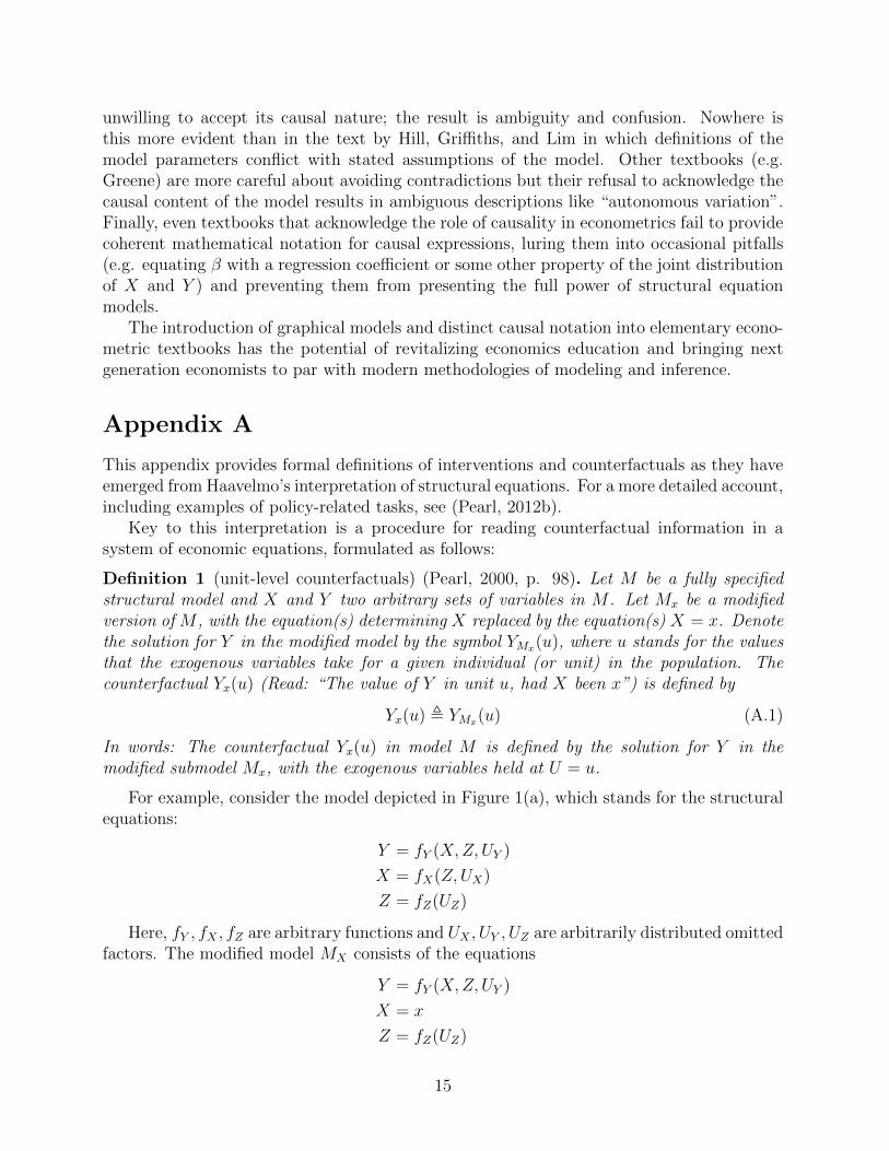
This appendix provides formal definitions of interventions and counterfactuals as they haveemerged from Haavelmo’s interpretation of structural equations. For a more detailed account,including examples of policy-related tasks, see (Pearl, 2012b).

Key to this interpretation is a procedure for reading counterfactual information in asystem of economic equations, formulated as follows:

Definition 1 (unit-level counterfactuals) (Pearl, 2000, p. 98). Let M be a fully specifiedstructural model and X and Y two arbitrary sets of variables in M . Let Mx be a modifiedversion of M , with the equation(s) determining X replaced by the equation(s) X = x. Denotethe solution for Y in the modified model by the symbol YMx(u), where u stands for the valuesthat the exogenous variables take for a given individual (or unit) in the population. Thecounterfactual Yx(u) (Read: “The value of Y in unit u, had X been x”) is defined by

Yx(u) , YMx(u) (A.1)

In words: The counterfactual Yx(u) in model M is defined by the solution for Y in themodified submodel Mx, with the exogenous variables held at U = u.

For example, consider the model depicted in Figure 1(a), which stands for the structuralequations:

Y = fY (X,Z, UY )

X = fX(Z,UX)

Z = fZ(UZ)

Here, fY , fX , fZ are arbitrary functions and UX , UY , UZ are arbitrarily distributed omittedfactors. The modified model MX consists of the equations

Y = fY (X,Z, UY )

X = x

Z = fZ(UZ)

15

(a) (b)

Figure 1

and is depicted in Figure 1b.The counterfactual Yx(u) at unit u = (uX , uY , uZ) would take the value Yx(u) = fY (x, fZ(uZ), uY ),

which can be computed from the model. When u is unknown, the counterfactual becomesa random variable, written Yx = fY (x, Z, UY ) with x treated as constant, and Z and UYrandom variables governed by the original model.

Clearly, the distribution P (Yx = y) depends on both the distribution of the exogenousvariables P (YX , UY , YZ) and on the functions fX , fY , fZ . In the linear case, however, theexpectation E[Yx] is rather simple. Writing

Y = aX + bZ + UY

X = cZ + UX

Z = UZ

gives

Yx = ax+ bZ + UY

and

E(Yx) = ax+ bE(Z)

Remarkably, the average effect of an intervention can be predicted without making anycommitment to functional or distributional form. This can be seen by defining an interven-tion operator do(x) as follows:

P (Y = y|do(x)) , P (Yx = y) , PMx(Y = y) (A.2)

In words, the distribution of Y under the intervention do(X = x) is equal to the distri-bution of Y in the modified model Mx, in which the dependence of Z on X is disabled (asshown in Figure 1b).

Accordingly, we can use Mx to define average causal effects:

Definition 2 (Average causal effect). The average causal effect of X on Y , denoted byE[Y |do(x)] is defined by

E[Y |do(x)] , E[Yx] = E[YMx ] (A.3)

16

Note that Definition 2 encodes the effect of interventions not in terms of the model’sparameters but in the form of a procedure that modifies the structure of the model. It thusliberates economic analysis from its dependence on parameteric representations and permitsa totally non-parametric calculus of causes and counterfactuals that makes the connectionbetween assumptions and conclusions explicit and transparent.

If we further assume that the exogenous variables (UX , UY , UZ) are mutually independent(but arbitrarily distributed) we can write down the post-intervention distribution immedi-ately, by comparing the graph of Figure 1b to that of Figure 1a. If the pre-intervention jointprobability distribution is factored into (using the chain rule):

P (x, y, z) = P (z)P (x|z)P (y|x, z) (A.4)

the post-intervention distribution must have the factor P (x|z) removed, to reflect the missingarrow in Figure 1b. This yields:

P (x, y, z|do(X = x0)) =

{P (z)P (y|x, z) if x = x0

0 if x 6= x0

In particular, for the outcome variable Y we have P (y|do(x)) =∑

z P (z)P (y|x, z), whichreflects the operation commonly known as “adjusting for Z” or “controlling for Z”. Likewise,we have E(Y |do(x)) =

∑z P (z)E(Y |x, z), which can be estimated by regression using the

pre-intervention data.In the simple model of Figure 1a the selection of Z for adjustment was natural, since Z

is a confounder that causes both X and Y . In general, the selection of appropriate sets foradjustment is not a trivial task; it can be accomplished nevertheless by a simple graphicalprocedure (called “backdoor”) once we specify the graph structure (Pearl, 2009, p. 79).

Equation A.1 constitutes a bridge between structural equation models and the poten-tial outcome framework advanced by (Neyman, 1923) and (Rubin, 1974), which takes thecontrolled randomized experiment as its guiding paradigm but encounters difficulties articu-lating modeling assumptions. Whereas structural models encode causal assumptions in theform of functional relationships among realizable economic variables, the potential outcomeframework requires those same assumptions to be encoded as conditional independenciesamong counterfactual variables, an intractible cognitive task.

Appendix B

This appendix provides supporting quotes for Table 1.

1. Does the author present example problems that require causal reasoning?Greene: “-What are the likely effects on labor supply behavior of proposed negativeincome taxes? [Ashenfelter and Heckman (1974).]-Does attending an elite college bring an expected payoff in lifetime expected incomesufficient to justify the higher tuition? [Krueger and Dale (2001) and Krueger (2002).]-Does a voluntary training program produce tangible benefits? Can these benefits beaccurately measured?” [Angrist (2001).]

17

-Do smaller class sizes bring real benefits in student performance? [Hanuschek (1999),Hoxby (2000), Angrist and Lavy (1999)] -Does the presence of health insurance induceindividuals to make heavier use of the health care system—is moral hazard a mea-surable problem? [Riphahn et al. (2003)]... -Does a monetary policy regime that isstrongly oriented toward controlling inflation impose a real cost in terms of lost outputon the U.S.s economy? [Cecchetti and Rich (2001)]-Did 2001’s largest federal tax cut in U.S. history contribute to or dampen the concur-rent recession? Or was it irrelevant? (Greene, 2012, p. 3)Hill, Griffiths, Lim: “A city council ponders the question of how much violent crimewill be reduced if an additional million dollars is spent putting uniformed police on thestreet.“The owner of a local Pizza Hut must decide how much advertising space to purchasein the local newspaper, and thus must estimate the relationship between advertisingand sales.“Louisiana State University must estimate how much enrollment will fall if tuition israised by $100 per semester, and thus whether its reveneu from tuition will rise or fall.“The CEO of Proctor & Gamble must estimate how much demand there will be in tenyears for the detergent Tide, and how much to invest in new plant and equipment.“A real estate developer must predict by how much population and income will in-crease to the south of Baton Rouge, Louisiana, over the next few years, and whetherit will be profitable to begin construction of a gambling casino and golf course.“You must decide how much of your savings will go into a stock fund, and how muchinto the money market. This requires you to make predictions of the level of eco-nomics activity, the rate of inflation, and interest rates over your planning horizon.”(Hill, Griffiths, and Lim, 2011, pg. 3)Stock, Watson: “Question #1: Does reducing class size improve elementary schooleducation?”(Stock and Watson, 2011, p. 2)“Question #2: Is there racial discrimination in the market for home loans?”(Stock andWatson, 2011, p. 3)“Question #3: How much do cigarette taxes reduce smoking?”(Stock and Watson,2011, p. 3)Wooldridge: “For example, in equation (1.3) we might hypothesis that wage, thewage that can be earned in legal employment, has no effect on criminal behavior.”(Wooldridge, 2000, pg. 5)

2. Does the author present example problems that require prediction?Hill, Griffiths, Lim: “How much would we predict the weekly expenditure on food tobe for a household with an income of $800 per week?” (Hill, Griffiths, and Lim, 2011,pg. 42)Stock, Watson: “Question #4: What will the rate of inflation be next year?”(Stockand Watson, 2011, p. 4)

3. Does the author state that the structural equation in the econometric modelis meant to capture a causal relationship?Greene: “The ultimate goal of the econometric model builder is often to uncover the

18

deeper causal connections through elaborate structural, behavior models.” (Greene,2012, pp. 5-6)“Econometrics and statistics have historically been taught, understood, and operatedunder the credo that ‘correlation is not causation.’ But, much of the still-growingfield of microeconometrics and some of what have been done in this chapter have beenadvanced as ‘causal modeling’.” (Greene, 2012, p. 251)“The technique of instrumental variables estimation has evolved as a mechanism fordisentangling causal influences... when the instrument is an outcome of a ‘naturalexperiment,’ true exogeneity is claimed... On the basis of a natural experiment, theauthors identify a cause-and-effect relationship that would have been viewed as beyondthe reach of regression modeling under earlier paradigms.” (Greene, 2012, p. 252)Has discussion on Granger causality, exogeneity, and endogenity on p. 318.Hill, Griffiths, Lim: No mention of causality.Kennedy: “Granger developed a special definition of causality which econometriciansuse in place of the dictionary definition; strictly speaking, econometricians should say‘Granger-cause’ in place of ‘cause’, but usually they do not.” (Kennedy, 2008, p. 63)Stock and Watson: “Suppose that βClassSize = −0.6. Then a reduction in class size oftwo students per class would yield a predicted change in test scores of (−0.6)× (−2) =1.2.; that is, you would predict that test scores would rise by 1.2 points as a resultof the reduction in class sizes by two students per class.”(Stock and Watson, 2011, p.108)“Internal validity has two components. First, the estimator of the causal effect shouldbe unbiased and consistent. For example, if βSTR...”(Stock and Watson, 2011, p. 313)Ruud: “In particular, remember that the conditional mean does not necessarily de-scribe a causal relationship running from the conditioning variables to the variableunder expectation. The conditional mean is merely a function of a joint probabilitydistribution. Furthermore, one should use the probability distribution to interpretthe conditional mean. If, in our earnings example, the theory describes the profile ofwages over a population of workers with different levels of experience, then we havebeen studying the appropriate conditional mean. If, however, the theory concerns thewage profile of an individual worker over a lifetime, then we may have the wrong con-ditional mean under analysis. Additional assumptions or inquiries must establish thatwe will average across individuals at a point in time to study individuals over time.”(Ruud, 2000, p. 110)Wooldridge: “We just saw in equation (2.2) that does measure the effect of x on y,holding all other factors (in u) fixed. As we will see in Section 2.5, we are only ableto get reliable estimators of and from a random sample of data when we make anassumption restricting how the unobservable u is related to the explanatory variablex.” (Wooldridge, 2000, p. 24)

4. Does the author define β by the equality, βX = E[Y |X]?Greene: States “The unknown parameters of the stochastic relationship yi = x

′

iβ + εiare the objects of estimation... The population regression is E[yi|xi] = x

′iβ, whereas

our estimate of E[yi|xi] is denoted yi = x′ib.” (Greene, 2012, p. 26). However the book

also mentions that E[Y |X] = βX only under assumption of exogeneity of independent

19

variable.Hill, Griffiths, Lim: “In order to investigate the relationship between expenditure andincome, we must build an economic model and then an econometric model that formsthe basis for a quantitative or empirical economic analysis. In our food expenditureexample, economic theory suggests that average weekly household expenditure on food,represented by the conditional mean E(y|x), depends on household income, x In mosteconomics textbooks, consumption or expenditure functions relating consumption toincome are depicted as linear functions, and we begin by assuming the same thing. Themathematical representation of our economic model of household food expenditure,depicted in Figure 2.2, is E(y|x) = µy|x = β1 + βx2. The conditional mean E(y|x) in(2.1) is called a simple regression function.” (Hill, Griffiths and Lim, 2011, pg. 42-43)Kennedy: “Some econometricians prefer to define the relationship between C and Ydiscussed earlier as the ’mean of C conditional on Y is f(Y ),’ written as E(C|Y ) =f(Y ). The conditional expectation interpretation can cause some confusion. Supposewages are viewed as a function of education, gender, and marriage status. Consideran unmarried male with 12 years of education. The conditional expectation of such aperson’s income is the value of y averaged over all unmarried males with 12 years ofeducation. This says nothing about what would happen to a particular individual’sincome if he were to get married. The coefficient on marriage status tells us what theaverage difference is between married and unmarried people, much of which may bedue to unmeasured characteristics that differ between married and unmarried people.A positive coefficient on marriage status tells us that married people have differentunmeasured characteristics that tend to cause higher earnings; it does not mean thatgetting married will increase one’s income. On the other hand, it could be argued thatgetting married creates economies in organizing one’s nonwork life, which enhancesearning capacity. This would suggest that getting married would lead to some increasein earnings, but in light of earlier comments, the coefficient on marriage status wouldbe an overestimate of this effect.” (Kennedy, 2008, p. 9)Stock and Watson: “The first part of Equation (4.5), β0 + β1Xi, is the populationregression line or the population regression function. This is the relationshipthat holds between Y and X on average over the population. Thus, if you knew thevalue of X, according to this population regression line you would predict that thevalue of the dependent variable, Y , is β0 + β1X.”(Stock and Watson, 2011, p. 110)

5. Does the author define the error term as being the difference between E[Y |x]and Y ?Hill, Griffiths, Lim: “This is called a random error term, and it is defined as e =y − E(y|x) = y − β1 − β2x...” (Hill, Griffiths, and Lim, 2011, pg. 46)

6. Does the author interpret the error term as omitted variables that (togetherwith X) determine Y ?Greene:“The term ε is a random disturbance, so named because it “disturbs” anotherwise stable relationship. The disturbance arises for several reasons, primarilybecause we cannot hope to capture every influence on an economic variable in a model,no matter how elaborate. The net effect, which can be positive or negative, of these

20

omitted factors is captured in the disturbance.” (Greene, 2012, p. 13)Kennedy:“The existence of the disturbance term is justified in three main ways...(1) Omission of the influence of innumerable chance events...(2) Measurement error...(3) Human indeterminancy...” (Kennedy, 2008, p. 3)Stock and Watson: “The term ui in Equation (4.5) is the error term. The error term

incorporates all of the factors responsible for the difference between the ith district’saverage test score and the value predicted by the population regression line. This errorterm contains all the other factors besides X that determine the value of the dependentvariable, Y , for a specific observation, i.”(Stock and Watson, 2011, p. 110)Wooldridge: Refers to u as “all other relevant factors”. (Wooldridge, 2000, pg. 14, pg.23)

7. Does the author state that the regression equation in the econometric modelis meant to capture a ceteris paribus or “everything else held fixed” rela-tionship?Greene: “The use of multiple regression involves a conceptual experiment that wemight not be able to carry out in practice, the ceteris paribus analysis familiar in eco-nomics.” (Greene, 2012, p. 36)Ruud: “These two components are analogous to the components of the total derivativeof a function of two variables f(x1, x2) with respect to the first variable: df(x1, x2)

dx1=

δf(x1, x2)δx1

+ dx2dx1

δf(x1, x2)δx2

. The first term is the ceteris paribus change in f for a change inx1 and the second term is the product of the ceteris paribus change in f for a changein x2 and the change in x2accompanying a change in x1. In this analogy, we interpretthe function f as E∗[y|x1n, x2n]...” (Ruud, 2000, pg. 495)Wooldridge: “You probably remember from introductory economics that most eco-nomic questions are ceteris paribus by nature. For example, in analyzing consumerdemand, we are interested in knowing the effect of changing the price of a good on itsquantity demanded, while holding all other factors fixed. If other factors are not heldfixed, then we cannot know the causal effect of a price change on quantity demanded...If we succeed in holding all other relevant factors fixed and then find a link betweenjob training and wages, we can conclude that job training has a causal effect on workerproductivity.” (Wooldridge, 2000, p. 14)

8. Does the author assume that exogeneity of X is inherent to the model?Textbooks sometimes introduce the concept of exogeneity by saying that X is “notrandom” (Hill, Griffiths, Lim, 2011, pg. 45), “fixed in repeated samples” (Kennedy,2008, p. 41) (Hill et al., 2011, p. 46), or “nonstochastic” (Greene, 2012, p. 23). Theseassumptions are described as being a part of the “simple linear regression model” (Hill,Griffiths, Lim, 2011, pg. 47), the “classical linear regression model” (Kennedy, 1992,pg. 134), or the “linear regression model” (Greene, 2012, p. 12). Hill, Griffiths, Limand Kennedy also write that the assumption of X not being random can be relaxedto ε being independent of X (Kennedy, 2008, p. 137) (Hill, Griffiths, Lim, 2011, pg.401-402).Wooldridge: “How can we hope to learn in general about ceteris paribus effect of x on

21

y, holding other factors fixed, when we are ignoring all those other factors? Section2.5 will show that we are only able to get reliable estimates of β0 and β1 from arandom sample of data when we make an assumption restricting how teh unobservableu is related to the explanatory variable x... We now turn to the crucial assumptionregarding how u and x are related. The crucial assumption is that the average valueof u does not depend on the value of x.” (Wooldridge, 2009, . 24-24)

9. Does the author make clear the difference in assumptions needed for an-swering causal as opposed to predictive problems?Stock, Watson: “Up to now, the discussion of multiple regression analysis has focusedon the estimation of causal effects. Regression models can be used for other pur-poses, however, including forecasting. When regression models are used for forecast-ing, concerns about external validity are very important, but concerns about unbiasedestimation of causal effects are not.”(Stock and Watson, 2011, p. 327)

10. Does the author have separate notation for E[Y |do(x)] and E[Y |x]?

11. Does the author have separate notation for the slope of the line associatedwith E[Y |X] and the slope of the line associated with E[Y |do(X)]?

Acknowledgments

This research was supported in parts by grants from NSF #IIS1249822 and #IIS1302448,and ONR #N000-14-09-1-0665 and #N00014-10-1-0933.

This survey benefited from discussions with J.H. Abbring, David Bessler, Olav Bjerkolt,William Greene, James Heckman, Michael Margolis, Rosa Matzkin, Paul A. Ruud, JamesStock, Lars P. Syll, Mark W. Watson, and Jeffrey M. Wooldridge. Errors of omission ormisjudgment are purely ours.

References

Balke, A. and Pearl, J. (1995). Counterfactuals and policy analysis in structural mod-els. In Uncertainty in Artificial Intelligence 11 (P. Besnard and S. Hanks, eds.). MorganKaufmann, San Francisco, 11–18.

Epstein, R. (1987). A History of Econometrics. Elsevier Science, New York.

Glymour, M. and Greenland, S. (2008). Causal diagrams. In Modern Epidemiology(K. Rothman, S. Greenland and T. Lash, eds.), 3rd ed. Lippincott Williams & Wilkins,Philadelphia, PA, 183–209.

Goldberger, A. (1992). Models of substance; comment on N. Wermuth, ‘On block-recursive linear regression equations’. Brazilian Journal of Probability and Statistics 61–56.

Greene, W. (2012). Econometric Analysis. 7th ed. Pearson Education, New Jersey.

22

Haavelmo, T. (1943). The statistical implications of a system of simultaneous equations.Econometrica 11 1–12. Reprinted in D.F. Hendry and M.S. Morgan (Eds.), The Founda-tions of Econometric Analysis, Cambridge University Press, 477–490, 1995.

Haavelmo, T. (1944). The probability approach in econometrics (1944)*. Supplementto Econometrica 12 12–17, 26–31, 33–39. Reprinted in D.F. Hendry and M.S. Morgan(Eds.), The Foundations of Econometric Analysis, Cambridge University Press, New York,440–453, 1995.

Heckman, J. (2000). Causal parameters and policy analysis in economics: A twentiethcentury retrospective. The Quarterly Journal of Economics 115 45–97.

Heckman, J. (2005). The scientific model of causality. Sociological Methodology 35 1–97.

Heckman, J. (2008). Econometric causality. International Statistical Review 76 1–27.

Heckman, J. (2010). Building bridges between structural and program evaluation ap-proaches to evaluating policy. Journal of Economic Literature 48 356–398.

Hill, R., Griffiths, W. and Lim, G. (2011). Principles of Econometrics. 4th ed. JohnWiley & Sons Inc., New York.

Hoover, K. (2009). Counterfactuals and causal structure. Available at SSRN 1477531 .

Huang, Y. and Valtorta, M. (2006). Pearl’s calculus of intervention is complete. InProceedings of the Twenty-Second Conference on Uncertainty in Artificial Intelligence(R. Dechter and T. Richardson, eds.). AUAI Press, Corvallis, OR, 217–224.

Keane, M. P. (2010). A structural perspective on the experimentalist school. Journal ofEconomic Perspectives 24 47–58.

Kennedy, P. (2008). A Guide to Econometrics. Sixth ed. MIT Press, Cambridge, MA.

Leamer, E. E. (2010). Tantalus on the road to asymptopia. Journal of Economic Perspec-tives 24 31–46.

Matzkin, R. (2007). Handbook of econometrics. Elsevier, Amsterdam.

Morgan, S. and Winship, C. (2007). Counterfactuals and Causal Inference: Methodsand Principles for Social Research (Analytical Methods for Social Research). CambridgeUniversity Press, New York, NY.

Nevo, A. and Whinston, M. D. (2010). Taking the dogma out of econometrics: Structuralmodeling and credible inference. Journal of Economic Perspectives 24 69–82.

Neyman, J. (1923). On the application of probability theory to agricultural experiments.Essay on principles. Section 9. Statistical Science 5 465–480.

Pearl, J. (1995). Causal diagrams for empirical research. Biometrika 82 669–710.

23

Pearl, J. (2000). Causality: Models, Reasoning, and Inference. Cambridge UniversityPress, New York. 2nd edition, 2009.

Pearl, J. (2009). Causality: Models, Reasoning, and Inference. 2nd ed. Cambridge Uni-versity Press, New York.

Pearl, J. (2012a). The causal foundations of structural equation modeling. In Handbookof Structural Equation Modeling (R. H. Hoyle, ed.). Guilford Press, New York. In press.

Pearl, J. (2012b). Trygve Haavelmo and the emergence of causal calculus. Tech. Rep. R-391, Department of Computer Science, University of California, Los Angeles, CA. Writtenfor Econometric Theory, special issue on Haavelmo Centennial.

Rubin, D. (1974). Estimating causal effects of treatments in randomized and nonrandomizedstudies. Journal of Educational Psychology 66 688–701.

Ruud, P. (2000). An Introduction to Classical Econometric Theory. Oxford UniversityPress, Oxford.

Shpitser, I. (2008). Complete Identification Methods for Causal Inference. Ph.D. thesis,Computer Science Department, University of California, Los Angeles, CA.

Shpitser, I. and Pearl, J. (2006). Identification of conditional interventional distri-butions. In Proceedings of the Twenty-Second Conference on Uncertainty in ArtificialIntelligence (R. Dechter and T. Richardson, eds.). AUAI Press, Corvallis, OR, 437–444.

Shpitser, I. and Pearl, J. (2008). Complete identification methods for the causal hier-archy. Journal of Machine Learning Research 9 1941–1979.

Simon, H. and Rescher, N. (1966). Cause and counterfactual. Philosophy and Science33 323–340.

Spirtes, P., Glymour, C. and Scheines, R. (1993). Causation, Prediction, and Search.Springer-Verlag, New York.

Stock, J. and Watson, M. (2011). Introduction to Econometrics. 3rd ed. Addison-Wesley,New York.

Tian, J. and Pearl, J. (2002). A general identification condition for causal effects. In Pro-ceedings of the Eighteenth National Conference on Artificial Intelligence. AAAI Press/TheMIT Press, Menlo Park, CA, 567–573.

Verma, T. (1993). Graphical aspects of causal models. Tech. Rep. R-191, UCLA, ComputerScience Department.

Verma, T. and Pearl, J. (1990). Equivalence and synthesis of causal models. In Pro-ceedings of the Sixth Conference on Uncertainty in Artificial Intelligence. Cambridge, MA.Also in P. Bonissone, M. Henrion, L.N. Kanal and J.F. Lemmer (Eds.), Uncertainty inArtificial Intelligence 6, Elsevier Science Publishers, B.V., 255–268, 1991.

24

Wermuth, N. (1992). On block-recursive regression equations. Brazilian Journal of Prob-ability and Statistics (with discussion) 6 1–56.

White, H. and Chalak, K. (2009). Settable systems: An extension of pearl’s causal modelwith optimization, equilibrium and learning. Journal of Machine Learning Research 101759–1799.

Wooldridge, J. (2009). Should instrumental vari-ables be used as matching variables? Tech. Rep.<https://www.msu.edu/∼ec/faculty/wooldridge/current%20research/treat1r6.pdf>,Michigan State University, MI.

25