Contents lists available at ScienceDirect

NeuroImage

journal homepage: www.elsevier.com/locate/neuroimage

Regression DCM for fMRI

Stefan Frässlea,⁎,1, Ekaterina I. Lomakinaa,b,1, Adeel Razic,d, Karl J. Fristonc, JoachimM. Buhmannb, Klaas E. Stephana,c

a Translational Neuromodeling Unit (TNU), Institute for Biomedical Engineering, University of Zurich & ETH Zurich, 8032 Zurich, Switzerlandb Department of Computer Science, ETH Zurich, 8032 Zurich, Switzerlandc Wellcome Trust Centre for Neuroimaging, University College London, London WC1N 3BG, United Kingdomd Department of Electronic Engineering, NED University of Engineering & Technology, Karachi, Pakistan

A R T I C L E I N F O

Keywords:Bayesian regressionDynamic causal modelingVariational BayesGenerative modelEffective connectivityConnectomics

A B S T R A C T

The development of large-scale network models that infer the effective (directed) connectivity among neuronalpopulations from neuroimaging data represents a key challenge for computational neuroscience. Dynamiccausal models (DCMs) of neuroimaging and electrophysiological data are frequently used for inferring effectiveconnectivity but are presently restricted to small graphs (typically up to 10 regions) in order to keep modelinversion computationally feasible. Here, we present a novel variant of DCM for functional magnetic resonanceimaging (fMRI) data that is suited to assess effective connectivity in large (whole-brain) networks. The approachrests on translating a linear DCM into the frequency domain and reformulating it as a special case of Bayesianlinear regression. This paper derives regression DCM (rDCM) in detail and presents a variational Bayesianinversion method that enables extremely fast inference and accelerates model inversion by several orders ofmagnitude compared to classical DCM. Using both simulated and empirical data, we demonstrate the facevalidity of rDCM under different settings of signal-to-noise ratio (SNR) and repetition time (TR) of fMRI data.In particular, we assess the potential utility of rDCM as a tool for whole-brain connectomics by challenging it toinfer effective connection strengths in a simulated whole-brain network comprising 66 regions and 300 freeparameters. Our results indicate that rDCM represents a computationally highly efficient approach withpromising potential for inferring whole-brain connectivity from individual fMRI data.

Introduction

The human brain is organized as a network of local circuits that areinterconnected via long-range fiber pathways, providing the structuralbackbone for the functional cooperation of distant specialized brainsystems (Passingham et al., 2002; Sporns et al., 2005). Understandingboth structural and functional integration among neuronal populationsis indispensable for deciphering mechanisms of both normal cognitionand brain disease (Bullmore and Sporns, 2009). Neuroimaging tech-niques, such as functional magnetic resonance imaging (fMRI), havecontributed substantially to this endeavor. While the early neuroima-ging era focused mainly on localizing cognitive processes in specificbrain areas (functional specialization), the last decade has seen afundamental shift towards the study of connectivity as the fundamentfor functional integration (Friston, 2002; Smith, 2012).

Three different aspects of brain connectivity are typically distin-guished. First, structural connectivity – that is, anatomical connections

such as long-range projections that make up white matter and linkcortical and subcortical regions. Structural connectivity is typicallyinferred from human diffusion-weighted imaging data or from tracttracing studies in animals. Second, functional connectivity describesinteractions among neuronal populations (brain regions) as statisticalrelations. Functional connectivity can be computed in numerous ways,including correlation, mutual information, or spectral coherence(Friston, 2011). Third, effective connectivity is based on a model ofthe interactions between neuronal populations and how the ensuingneuronal dynamics translate into measured signals.

While structural and functional connectivity methods have pro-vided valuable insights into the wiring and organization of the humanbrain both in health and disease (for reviews, see Buckner et al., 2013;Bullmore and Sporns, 2009; Fornito et al., 2015; Sporns et al., 2005),they are essentially descriptive and do not allow for mechanisticaccounts of a neuronal circuit – that is, what computations areperformed and how they are implemented physiologically. By contrast,

http://dx.doi.org/10.1016/j.neuroimage.2017.02.090Received 6 November 2016; Accepted 28 February 2017

⁎ Corresponding author at: Translational Neuromodeling Unit (TNU), Institute for Biomedical Engineering, University of Zurich & ETH Zurich, Wilfriedstrasse 6, 8032 Zurich,Switzerland.

1 Contributed equally to this work.E-mail address: stefanf@biomed.ee.ethz.ch (S. Frässle).

NeuroImage 155 (2017) 406–421

Available online 01 March 20171053-8119/ © 2017 The Authors. Published by Elsevier Inc. This is an open access article under the CC BY-NC-ND license (http://creativecommons.org/licenses/BY-NC-ND/4.0/).

MARK

models of effective connectivity that rest upon a generative model can,in principle, infer upon the latent (neuronal or computational)mechanisms that underlie measured brain activity. In other words,models of effective connectivity seek explanations of the data, notstatistical characterizations. This is not only fundamentally importantfor basic neuroscience, but also offers tremendous opportunities forclinical applications (Stephan et al., 2015).

The last decade has seen enormous interest and activity in devel-oping methods for inferring directed connection strengths from fMRIdata, such as Granger causality (GC; Roebroeck et al., 2005) anddynamic causal modeling (DCM; Friston et al., 2003). While GCoperates directly on the data and quantifies connectivity in terms oftemporal dependencies, DCM rests on a generative model, allowing forinference on latent neuronal states that cause observations (Fristonet al., 2013). While these methods have already made fundamentalcontributions to our understanding of functional integration in thehuman brain, existing methods are still subject to major limitations(for reviews on strengths and challenges of models of effectiveconnectivity, see Daunizeau et al., 2011a; Friston et al., 2013;Stephan and Roebroeck, 2012; Valdes-Sosa et al., 2011). For example,there is a fundamental trade-off between the complexity of a model andparameter estimability: while biophysical network models (BNMs)capture many anatomical and physiological details (Deco et al.,2013a; Jirsa et al., 2016), their nonlinear functional forms, very largenumber of parameters, and pronounced parameter interdependenciesusually render parameter estimation an extremely challenging compu-tational problem (for discussion, see Stephan et al., 2015). At present,large-scale BNMs are therefore usually used for simulating data, asopposed to inferring the strength of individual connections.

In contrast to biophysical network models, generative models likeDCM rest on a forward model (from hidden neuronal circuit dynamicsto measured data) that is inverted using Bayesian principles in order tocompute the posterior probability distributions of the model para-meters (model inversion). To render this challenge computationallyfeasible, DCM typically deals with small networks consisting of no morethan 10 regions (but see Seghier and Friston, 2013) whose activity hasbeen perturbed by carefully designed experimental manipulations.DCM for fMRI has also been extended to cover resting state fMRItime series by modelling endogenous fluctuations in neuronal activity.These neuronal fluctuations can be treated as hidden or latent neuronalstates (leading to stochastic DCM; Daunizeau et al., 2009).Alternatively, the second order statistics of neuronal fluctuations canbe treated deterministically within DCM for cross-spectral responses(Friston et al., 2014a). Irrespective of the particular form of DCM, therestriction to a small number of nodes can be a major limitation; forexample, for clinical applications concerned with whole-brain physio-logical phenotyping of patients in terms of directed connectivity.

In this paper, we introduce a novel variant of DCM for fMRI thathas the potential to overcome this bottleneck and is suitable, inprinciple, to assess effective connectivity in large (whole-brain) net-works. Put simply, the approach rests upon shifting the formulation ofDCM from the time to the frequency domain and casting modelinversion as a problem of Bayesian regression. More specifically, wereformulate the neuronal state equation of a linear DCM in the timedomain as an algebraic expression in the frequency domain. Thistransformation rests on solving differential equations using the Fouriertransformation. Using this approach from the signal processingliterature (e.g., Bracewell, 1999; Oppenheim et al., 1999), we showthat – under a few assumptions and modifications to the originalframework – the problem of model inversion in DCM for fMRI can becast as a special case of a Bayesian linear regression problem (Bishop,2006). This regression DCM (rDCM) is computationally extremelyefficient, enabling its potential use for inferring effective connectivity inwhole-brain networks. Note that rDCM is conceptually not unrelated toDCM for cross-spectral responses mentioned above in the sense thatboth approaches use spectral data features. However, rDCM is formally

distinct from cross-spectral DCM because it models the behavior ofeach system node (in the frequency domain) rather than the crossspectral density as a compact summary (of functional connectivityamong system nodes).

In what follows, we first introduce the theoretical foundations ofrDCM and highlight where the approach deviates from the standardDCM implementation. We then demonstrate the face validity andpractical utility of rDCM for a small six-region network, testing therobustness of both parameter estimation and model selection underrDCM using simulations and an empirical fMRI dataset on faceperception (Frässle et al., 2016b, 2016c). Having established thevalidity of rDCM for small networks, we then proceed to simulationsthat provide a proof-of-principle for the utility of rDCM for assessingeffective connectivity in large networks. The simulations use a whole-brain parcellation (66 regions) and empirical connectivity matrix thatwas introduced by Hagmann et al. (2008) and has been used by severalmodeling studies since (e.g., Deco et al., 2013b; Honey et al., 2009),resulting in a model with 300 free parameters.

Methods and materials

Dynamic causal modeling

DCM is a generative modeling framework for inferring hiddenneuronal states from measured neuroimaging data by quantifying theeffective (directed) connectivity among neuronal populations (Fristonet al., 2003). Specifically, DCM explains changes in neuronal popula-tion dynamics as a function of the network’s connectivity (endogenousconnectivity A) and some experimental manipulations. These experi-mental manipulations uj can either directly influence neuronal activityin the network’s regions (driving inputs C) or perturb the strength ofthe endogenous connections among regions (modulatory influences B).This can be cast in terms of the following bilinear state equation:

⎛⎝⎜⎜

⎞⎠⎟⎟∑dx

dtA u B x Cu= + +

j

m

jj

=1

( )

(1)

This neuronal model is then coupled to a weakly nonlinearhemodynamic forward model that maps hidden neuronal dynamicsto observed BOLD signal time series (Buxton et al., 1998; Friston et al.,2000; Havlicek et al., 2015; Stephan et al., 2007). In brief, thehemodynamic model describes how changes in neuronal states inducechanges in cerebral blood flow, blood volume and deoxyhemoglobincontent. The latter two variables enter an observation equation to yielda predicted BOLD response. For reviews on the biophysical andstatistical foundations, see Daunizeau et al. (2011a) and Friston et al.(2013).

Inference proceeds in a fully Bayesian setting, using an efficientvariational Bayesian approach under the Laplace approximation (VBL)– meaning that prior and posterior densities are assumed to have aGaussian fixed form (Friston et al., 2007). This scheme provides twoestimates: (i) The sufficient statistics of the posterior distributions ofmodel parameters (i.e., conditional mean and covariance), and (ii) thenegative free energy, a lower-bound approximation to the log modelevidence (i.e., the probability of the data given the model). The negativefree energy provides a principled trade-off between a model’s accuracyand complexity, and serves as a measure for testing competing models(hypotheses) about network architecture by means of Bayesian modelcomparison (Penny et al., 2004; Stephan et al., 2009a).

Regression DCM

Neuronal state equation in frequency domainIn this section, we introduce a new formulation of DCM that

essentially reformulates model inversion as a special case of Bayesianlinear regression (for further details of the derivation, see Lomakina,

S. Frässle et al. NeuroImage 155 (2017) 406–421

407

2016). We thus refer to this approach as regression DCM (rDCM). Thisapproach rests on several modifications of the original DCM imple-mentation that include: (i) translation from the time domain to thefrequency domain, (ii) linearizing the hemodynamic forward model,(iii) assuming partial independence between connectivity parameters,and (iv) using a Gamma prior for noise precision. These changes allowus to derive an algebraic expression for the likelihood function and avariational Bayesian scheme for inference, which convey a highlysignificant increase in computational efficiency by several orders ofmagnitude. This potentially enables a number of innovative applica-tions – most importantly, it renders rDCM a promising tool forstudying effective connectivity in whole-brain networks. The massiveincrease in computational efficiency afforded by rDCM rests on the factthat standard (VBL) inversion schemes require one to integrate adeterministic system of neuronal dynamics to produce a predicted(hemodynamic) response. This integration can be computationallydemanding, especially for long time series. The beauty of summarizinga time series (and underlying latent states) with its Fourier transform isthat one eludes the problem of solving differential equations, enablingthe solution of a compact, static regression model.

In this initial paper, we focus on the simplest case – a linear DCM –because bilinear models aggravate the derivation of an algebraicexpression for the likelihood function (but see the Discussion forpotential future extensions of rDCM). Linear DCMs are described bythe following neuronal state equation

dxdt

Ax Cu= +(2)

This differential equation can be translated to the frequency domainby means of a Fourier transformation. As the Fourier transform is alinear operator, this results in the following expression

dxdt

Ax Cu= +(3)

where the Fourier transform is denoted by the hat symbol. We can nowapply the differential property of the Fourier transform

dxdt

iωx=(4)

where i = ± −1 is the imaginary number and ω the Fourier coordi-nate. Substituting Eq. (4) into Eq. (3) leads to the representation of theneuronal state equation as an algebraic system in the frequencydomain:

iωx Ax Cu= + (5)

The system described in Eq. (5) is still linear with respect to themodel parameters, and the meaning of the parameters is preserved.

Observation model and measurement noiseHaving re-expressed the neuronal state equation in the frequency

domain, we now turn to the observation model that links hiddenneuronal dynamics to measured BOLD signals. In classical DCM, theobservation model consists of a cascade of nonlinear differentialequations describing the hemodynamics and a nonlinear static BOLDsignal equation (Friston et al., 2000; Stephan et al., 2007). Thesenonlinearities pose a problem for our approach because they prevent astraightforward translation to the frequency domain. One possibilitywould be to linearize these equations (as in Stephan et al., 2007). Inthis initial paper, however, we adopt a simpler approach: convolutionwith a fixed hemodynamic response function (HRF). Multiplying Eq.(5) with the Fourier transform of the HRF and making use of the factthat a multiplication of the Fourier transforms of two functions isequivalent to the Fourier transform of the convolution of these twofunctions, one arrives at the following algebraic system:

iω h x A h x Ch u

iωy Ay Ch u

( ⊗ ) = ( ⊗ ) +

= +B B (6)

Here, ⊗ denotes the convolution and yB is the deterministic (noise-free) prediction of the data. However, Eq. (6) is not an accuratedescription for measured fMRI data, for two reasons: First, while theneuronal activity x and BOLD response yB are continuous signals, ourmeasurements or observations are discrete. Second, measured fMRIdata is inevitably affected by noise.

To account for the discrete nature of the data (and the fact thatcomputers can only represent discrete rather than continuous data), weuse a discretized version of Eq. (6). This necessitates the use of thediscrete Fourier transform (DFT) and the discretization of frequencyand time:

⎛⎝⎜

⎞⎠⎟m miω i ω πi

NT Te:= Δ = 2 ≈ 1 −1

mπi N2

(7)

where N represents the number of data points, T the time intervalbetween subsequent points, ωΔ the frequency interval, andm N= [0,1, …, − 1] a vector of frequency indices. In Eq. (7), we havemade use of a linear approximation to the exponential function toobtain the final expression, which is also known as the differenceoperator of the DFT. Plugging Eq. (7) into Eq. (6) leads to the discreterepresentation of the (deterministic) BOLD equation in the frequencydomain:

⎛⎝⎜

⎞⎠⎟e

yT

Ay Ch u−1 = +mπi N B

B2

(8)

where the hat symbol now denotes the discrete Fourier transform.Having obtained an expression for discrete data, we now augment

the model with observation or measurement noise. Here, similar to thesetting in classical DCM, we assumed the measurement noise to bewhite for each region i R=[1, …, ] (or, more precisely, the hemodynamicresponses at each region to be whitened following an estimation oftheir temporal autocorrelations) with region-specific noise variancesσi

2:

y y σ I= + ϵ , ϵ ~ (0, )i B i i i i N N,2

× (9)

where IN N× is the identity matrix. Inserting Eq. (9) into Eq. (8) gives anexpression for the measured fMRI signal

⎛⎝⎜

⎞⎠⎟e y

TAy Ch u υ−1 = + +

mπi N2

(10)

The form of Eq. (10) is reminiscent of structural equation models(McIntosh, 1998) and multivariate autoregressive models (Roebroecket al., 2005) in the frequency domain. In Eq. (10), υ is a noise vector ofthe following form:

⎛⎝⎜

⎞⎠⎟υ e

TA= −1 ϵ̂ − ϵ̂

mπi N2

(11)

While υ also has white noise properties, its dependence on theendogenous connectivity parameters (A matrix) complicates the deri-vation of an analytical expression for the likelihood function. Wecircumvent this problem by an approximation, introducing a partialindependence assumption that regards υi as an independent randomvector with a noise precision parameter τi. This approximation meansthat potential dependencies amongst parameters affecting differentregions are discarded (i.e., interdependencies are only considered forparameters entering the same region). Effectively, this constitutes amean field approximation in which the (approximate) posteriorfactorizes among sets of connections providing inputs to each node.This assumption allows for an extremely efficient (variational) inver-sion of our DCM. Heuristically, because DCM models changes inactivity caused by hidden states in other regions, this approximationmeans that Eq. (10) can estimate the strengths of connections to any

S. Frässle et al. NeuroImage 155 (2017) 406–421

408

given region by, effectively, minimizing the difference between ob-served changes in responses and those predicted by observed activityelsewhere.

Given this approximation, we can re-write Eq. (10) as a standardmultiple linear regression problem:

Y Xθ υ υ υ τ I= + , ~ ( ;0, )N N−1

× (12)

Here, we have defined Y as the dependent variable, X as the designmatrix (set of regressors) and θ as the parameter vector as follows:

⎛⎝⎜

⎞⎠⎟

∏p Y θ τ X Y Xθ τ I

Y eyT

X y y y h u h u h u

θ a a a c c c

( | , , ) = ( ; , )

:= −1

:= [ , ,…, , , ,…, ]

:= [ , ,…, , , ,…, ]

mi

R

i i i N N

iπi N i

R K

i i i iR i i iK

=1

−1×

2

1 2 1 2

1 2 1 2 (13)

where yi represents the measured signal in region i and uk the kthexperimental input to that region.

This derivation completes the reformulation of a linear DCM in thetime domain as a general linear model (GLM) in the frequency domain.The resulting algebraic expression in Eq. (12) offers many advantages,such as extremely efficient computation and exploitation of existingstatistical solutions. The transfer to the frequency domain also meansthat we can exploit knowledge about the frequencies that contain usefulinformation in fMRI; these are constrained by the low-pass filterproperties of neurovascular coupling and the sampling frequency (cf.Nyquist theorem), respectively. This means that sampling rate (TR)becomes an important factor, something that will be considered in oursimulations below.

Specification of regression DCM as a generative modelIn order to turn the GLM in Eq. (12) into a full generative model

(Bayesian regression), we need to specify priors for parameters andhyperparameters. While we keep the zero-mean Gaussian shrinkagepriors on connectivity parameters from classical DCM, we chose aGamma prior on the noise precision τ (not a log-normal prior as inclassical DCM). This change was motivated by the fact that Gammapriors serve as conjugate priors on precision for a Gaussian likelihood,which simplifies the derivation of an expression for the posterior:

p θ θ μ π exp

p τ Gamma τ α ββα

τ exp

( ) = ( ; , Σ ) = (2 ) Σ

( ) = ( ; , ) =Γ( )

i ii i

Di θ μ θ μ

i i

α

iα β τ

0 0− 2 0

− 12 − 1

2 ( − ) Σ ( − )

0 00

0

−1 −

ii

i T ii

i

i

0 0−1

0

00 0

(14)

Here, μ0 and Σ0 are the mean and covariance of the Gaussian prioron connectivity parameters, α0 and β0 are the shape and rateparameters of the Gamma prior on noise precision, and Γ is theGamma function. In this paper, we adopted the standard neuronalpriors from DCM10 as implemented in the Statistical ParametricMapping software package SPM8 (version R4290; www.fil.ion.ucl.ac.uk/spm). For the noise precision, we used α =20 and β =10 to match theGamma distribution closely to the first two moments of the standardlog-normal prior from DCM10.

Under this choice of priors, the posterior distribution over connec-tions to each region i and for the entire model, respectively, then takesthe form:

∏ ∏

p θ τ Y X p Y X θ τ p θ p τ

p θ τ Y X p Y X θ τ p θ p τ

( , , ) ∝ ( , , ) ( ) ( )

( , , ) ∝ ( , , ) ( ( ) ( ))

i i i i i i i i

i

R

i i ii

R

i i=1 =1 (15)

As already highlighted above, the formulation of rDCM represents aspecial case of Bayesian linear regression (Bishop, 2006). If the noiseprecision were known, Eq. (15) could be solved exactly. Since rDCMdoes not make this assumption, an analytical solution is not possible

and approximate inference procedures are needed instead. Here, wechose a variational Bayesian approach under the Laplace approxima-tion (VBL; compare Friston et al., 2007) to derive an iterativeoptimization scheme.

Variational Bayes: a brief summaryThis section provides a summary of variational Bayes (VB) that

hopes to enable readers with limited experience in variational Bayes tofollow the derivation of the update equations for rDCM below.Comprehensive introductions to VB can be found elsewhere (e.g.,Bishop, 2006). Generally speaking, VB is a framework for transformingintractable integrals into tractable optimization problems. The mainidea of this approach is to approximate the true posterior p θ τ y m( , , )by a simpler distribution q θ τ y m( , , ). For VBL, q θ τ y m( , , ) is assumedto have a Gaussian form and can thus be fully described by its sufficientstatistics – that is, the conditional mean and covariance (Friston et al.,2007).

Given such an approximate density, VB allows for achieving twothings simultaneously: (i) model inversion, i.e., estimating the bestapproximation to the true posterior (under the chosen form of q), and(ii) obtaining an approximation to the log model evidence (the basis forBayesian model comparison). This can be seen by decomposing the logmodel evidence as follows:

∬

∬

∬

∬

p y m q θ τ y m p y m q θ τ y mq θ τ y m

dθdτ

q θ τ y m p y θ τ m q θ τ y mp θ τ y m q θ τ y m

dθdτ

q θ τ y m p y θ τ mq θ τ y m

dθdτ

q θ τ y m q θ τ y mp θ τ y m

dθdτ

F KL q θ τ y m p θ τ y m

ln ( ) = ( , , ) ln ( ) ( , , )( , , )

= ( , , ) ln ( , , ) ( , , )( , , ) ( , , )

= ( , , ) ln ( , , )( , , )

+ ( , , ) ln ( , , )( , , )

= + [ ( , , ) ( , , )] (16)

where F is known as the negative free energy and the second term isthe Kullback-Leibler (KL) divergence between the approximate poster-ior and the true posterior density. Because the KL divergence is alwayspositive or zero (Mackay, 2003), the negative free energy provides alower bound on the log model evidence. The KL term can thus beminimized (implicitly) by maximizing the negative free energy. Thelatter is feasible because F does not depend on the true (but unknown)posterior, but only on the approximate posterior (see Eq. (16)), and canbe maximized by gradient ascent (with regard to the sufficient statisticsof q).

To facilitate finding the q that maximizes F , a mean field approx-imation to q θ τ y m( , , ) is typically chosen. For example, one mightassume that q factorizes into marginal posterior densities of para-meters and hyperparameters:

q θ τ y m q θ y m q τ y m( , , ) = ( , ) ( , ) (17)

Under this mean field approximation, the approximate marginalposteriors that maximize F can be found by iteratively applying thefollowing two update equations

q θ y m p y θ τ m

q τ y m p y θ τ m

( , ) = exp[ ln ( , , ) ]

( , ) = exp[ ln ( , , ) ]q τ y m

q θ y m

( , )

( , ) (18)

where · q denotes the expectation with respect to q. While deriving theright-hand side terms (the so-called “variational energies”) can becomplicated, once known they enable a very fast optimization scheme.

Variational Bayes for regression DCMHaving outlined the basic concepts of variational Bayes, we now present

an efficient VBL approach for rDCM, which results in a set of analyticalupdate equations for the model parameters and an expression for thenegative free energy. Under the VBL assumptions, update equations forq θ Y X( , ) and q τ Y X( , ) – that is, for connectivity parameters and noise

S. Frässle et al. NeuroImage 155 (2017) 406–421

409

precision, respectively – can be derived as shown by Eqs. (19) and (20).Given the mean field approximation or factorization of the approx-

imate posterior over subsets of connections (see above), optimizationcan be performed for each region independently. Technically, thisenables us to dissolve the problem of inverting a full adjacency matrixof endogenous connectivity strengths into a series of variationalupdates in which the posterior expectations of each subset (rows ofthe A matrix) are optimized successively. Hence, without loss ofgenerality, we restrict the following derivation of the update equationsto a single region.

Update equation of θ:

⎛⎝⎜⎜

⎞⎠⎟⎟

⎛⎝⎜⎜

⎞⎠⎟⎟

q θ Y X p θ τ Y X const

Y Xθ τ I θ μ const

τY Xθ Y Xθ θ μ θ μ const

αβ

θ X Xθαβ

θ X Y θ θ θ μ const

θαβ

X X θ θαβ

X Y μ const

ln ( , ) = ln ( , , ) +

= ln ( ; , ) + ln ( ; , Σ ) +

= −2

( − ) ( − ) − 12

( − ) Σ ( − ) +

= −2

+ − 12

Σ + Σ +

= − 12

+ Σ + + Σ +

q τ

N N q τ

q τ T T

τ y

τ y

T T τ y

τ y

T T T T

T τ y

τ y

T T τ y

τ y

T

( )−1

× 0 0 ( )

( )0 0

−10

0−1

0−1

0

0−1

0−1

0

(19)

where Σ0−1 is the inverse prior covariance matrix on connectivity

parameters, and ατ y and βτ y are the posterior shape and rateparameters of the Gamma distribution on noise precision, respectively.Here, we made use of τ =q τ

α

β( )τ y

τ y, with · denoting the expected value,

and the fact that all terms independent of θ can be absorbed by theconstant term.

Update equation of τ:

q τ Y X p θ τ Y X const

Y Xθ τ I Gamma τ α β const

N τ τ Y Xθ Y Xθ α τ β τ const

N τ τ θ X Xθ θ X Y Y Y α τ β τ const

N τ τ Y Xμ Y Xμ τ trace X X α τ

β τ const

ln ( , ) = ln ( , , ) +

= ln ( ; , ) + ln ( ; , ) +

=2

ln −2

( − ) ( − ) + ( −1) ln − +

=2

ln −2

−2 + + ( −1) ln − +

=2

ln −2

( − ) ( − ) −2

( Σ ) + ( −1) ln

− +

q θ

N N q θ

Tq θ

T T T T Tq θ

θ yT

θ yT

θ y

( )−1

× 0 0 ( )

( ) 0 0

( ) 0 0

0

0

(20)

where N is the number of data points, and μθ y and Σθ y are the meanand covariance of the posterior (Gaussian) density on connectivityparameters, respectively. Here, we made use of θ μ=q θ θ y( ) and thefact that all terms independent of τ can be absorbed by the constantterm. Comparing Eqs. (19) and (20) to the logarithm of the multi-variate normal distribution and to the logarithm of the Gammadistribution, respectively, allows one to derive a set of simple updateequations for the sufficient statistics of the approximate posteriordensities q θ Y X( , ) and q τ Y X( , ).

Final iterative scheme:

⎛⎝⎜⎜

⎞⎠⎟⎟

⎛⎝⎜⎜

⎞⎠⎟⎟

⎛⎝⎜

⎞⎠⎟

⎛⎝⎜

⎞⎠⎟

αβ

X X

μαβ

X Y μ

α α N

β β Y Xμ Y Xμ trace X X

Σ = + Σ

= Σ + Σ

= +2

= + 12

− − + 12

( Σ )

θ yτ y

τ y

T

θ y θ yτ y

τ y

T

τ y

τ y θ y

T

θ yT

θ y

0−1

−1

0−1

0

0

0 (21)

Since the update equations for q θ Y X( , ) and q τ Y X( , ) are mutuallydependent on each other, we iterate their updates until convergence toobtain the optimal approximate distributions. More precisely, in thecurrent implementation of rDCM, the iterative scheme proceeds untilthe change in τ falls below a specified threshold (i.e., 10-10). In futureimplementations, we will explore the utility of using changes invariational free energy within each iteration as the criterion forconvergence (for comparison, VBL typically uses a change in freeenergy of 1/8 or less to terminate the iterations).

Having obtained expressions for the approximate posteriordensities for the connectivity and noise parameters, one can derivean expression for the negative free energy F . As described above, Fserves as a lower-bound approximation to the log model evidencewhich represents a measure of the “goodness” of a model, takinginto account both its accuracy and complexity (Friston et al., 2007;Mackay, 1992; Penny et al., 2004; Stephan et al., 2009a). F is thusroutinely used to formally compare different candidate models anddecide which of them provides the most plausible explanation forthe observed data (Bayesian model selection, BMS). To do so, oneneeds to compute the actual value of F, given the data and (acurrent estimate of the) approximate posterior; the followingequations show how this is done in the case of rDCM.

As can be seen from Eq. (16), the negative free energy can be cast interms of the difference of the expected energy of the system (i.e., log-joint) and the entropy of the approximate posterior:

⎡⎣⎢

⎤⎦⎥∬F max q θ τ Y X q θ τ Y X

p θ τ Y Xdθdτ

p θ τ Y X q θ τ Y X

p Y θ τ X p θ p τ

q θ Y X q τ Y X

= − ( , , ) ln ( , , )( , , )

= ln ( , , ) − ln ( , , )

= ln ( , , ) + ln ( ) + ln ( )

− ln ( , ) − ln ( , )

q θ τ Y X

q θ τ q θ τ

q θ τ q θ τ q θ τ

q θ τ q θ τ

( , , )

( , ) ( , )

( , ) ( , ) ( , )

( , ) ( , ) (22)

In the following, we outline the derivation of the individualcomponents of the negative free energy (see Lomakina, 2016):

Expectation of the likelihood:

⎛⎝⎜

⎞⎠⎟

⎛⎝⎜

⎞⎠⎟

⎛⎝⎜

⎞⎠⎟

p Y θ τ X Y Xθ τ I

N π τ I τ Y Xθ Y Xθ

N π N ττ

Y Xθ Y Xθ

N π N α βαβ

Y Xμ Y Xμ

αβ

trace X X

ln ( , , ) = ln ( ; , )

= −2

ln 2 − 12

ln −2

( − ) ( − )

= −2

ln 2 +2

ln −2

( − ) ( − )

= −2

ln 2 +2

Ψ( ) − ln −2

− −

−2

( Σ )

q θ τ N N q θ τ

N NT

q θ τ

q τq τ T

q θ

τ y τ yτ y

τ yθ y

T

θ y

τ y

τ y

Tθ y

( , )−1

× ( , )

−1×

( , )

( )( )

( )

(23)

where Ψ denotes the digamma function.

Expectation of the prior on θ:

⎛⎝⎜

⎞⎠⎟

⎛⎝⎜

⎞⎠⎟

p θ θ μ

D π θ μ θ μ

D π θ μ θ μ

D π μ μ μ μ

trace

ln ( ) = ln ( ; , Σ )

= −2

ln 2 − 12

ln Σ − 12

( − ) Σ ( − )

= −2

ln 2 − 12

ln Σ − 12

( − ) Σ ( − )

= −2

ln 2 − 12

ln Σ − 12

− Σ −

− 12

(Σ Σ )

q θ τ q θ τ

T

q θ

Tq θ

θ y

T

θ y

θ y

( , ) 0 0 ( , )

0 0 0−1

0( )

0 0 0−1

0 ( )

0 0 0−1

0

0−1

(24)

where D is the number of connections entering the region.

S. Frässle et al. NeuroImage 155 (2017) 406–421

410

Expectation of the prior on τ :

⎛⎝⎜

⎞⎠⎟

p τ Gamma τ α β

α β α α τ β τ

α β α α τ β τ

α β α α α β βαβ

ln ( ) = ln ( ; , )

= ln − ln Γ( ) + ( −1) ln −

= ln − ln Γ( ) + ( −1) ln −

= ln − ln Γ( ) + ( −1) Ψ( ) − ln −

q θ τ q θ τ

q τ

q τ q τ

τ y τ yτ y

τ y

( , ) 0 0 ( , )

0 0 0 0 0 ( )

0 0 0 0 ( ) 0 ( )

0 0 0 0 0

(25)

where Γ is the Gamma function.

Entropy of θ:

⎞⎠⎟

⎛⎝⎜

⎞⎠⎟

⎛⎝⎜

⎞⎠⎟

⎛⎝⎜

⎞⎠⎟

⎛⎝⎜

⎞⎠⎟

⎛⎝⎜

⎞⎠⎟

⎛⎝⎜

⎞⎠⎟

q θ Y X θ μ

D π θ μ θ μ

D π θ μ θ μ

D π μ μ μ μ

trace

D π

− ln ( | , ) = − ln ( ; , Σ

= − −2

ln 2 − 12

ln Σ − 12

− Σ −

=2

ln 2 + 12

ln Σ + 12

− Σ −

=2

ln 2 + 12

ln Σ + 12

− Σ −

+ 12

(Σ Σ )

=2

(1+ ln 2 ) + 12

ln Σ

q θ τ θ y θ yq θ τ

θ y θ y

T

θ y θ yq θ

θ y θ y

T

θ y θ yq θ

θ y θ y θ y

T

θ y θ y θ y

θ y θ y

θ y

( , )( , )

−1

( )

−1

( )

−1

−1

(26)

Entropy of τ:

⎛⎝⎜

⎞⎠⎟

⎛⎝⎜

⎞⎠⎟

q τ Y X Gamma τ α β

α β α α τ β τ

α β α α τ β τ

α α β α α α β

α β α α α

− ln ( , ) = − ln ; ,

= − ln − ln Γ( ) + ( −1) ln −

= − ln + ln Γ( ) − ( −1) ln +

= − ln + ln Γ( ) − ( −1) Ψ( ) − ln

= − ln + ln Γ( ) − ( −1)Ψ( )

q θ τ τ y τ yq θ τ

τ y τ y τ y τ y τ yq τ

τ y τ y τ y τ y τ y q τ

τ y τ y τ y τ y τ y τ y τ y

τ y τ y τ y τ y τ y

( , )( , )

( )

q(τ) ( )

(27)

Summing up the components from Eqs. (23)–(27) yields anestimate of the negative free energy for each individual region. Thenegative free energy for the full model can then be computed bysumming over all regions of the model

∑F F=i

R

i=1 (28)

Synthetic data: six-region DCM

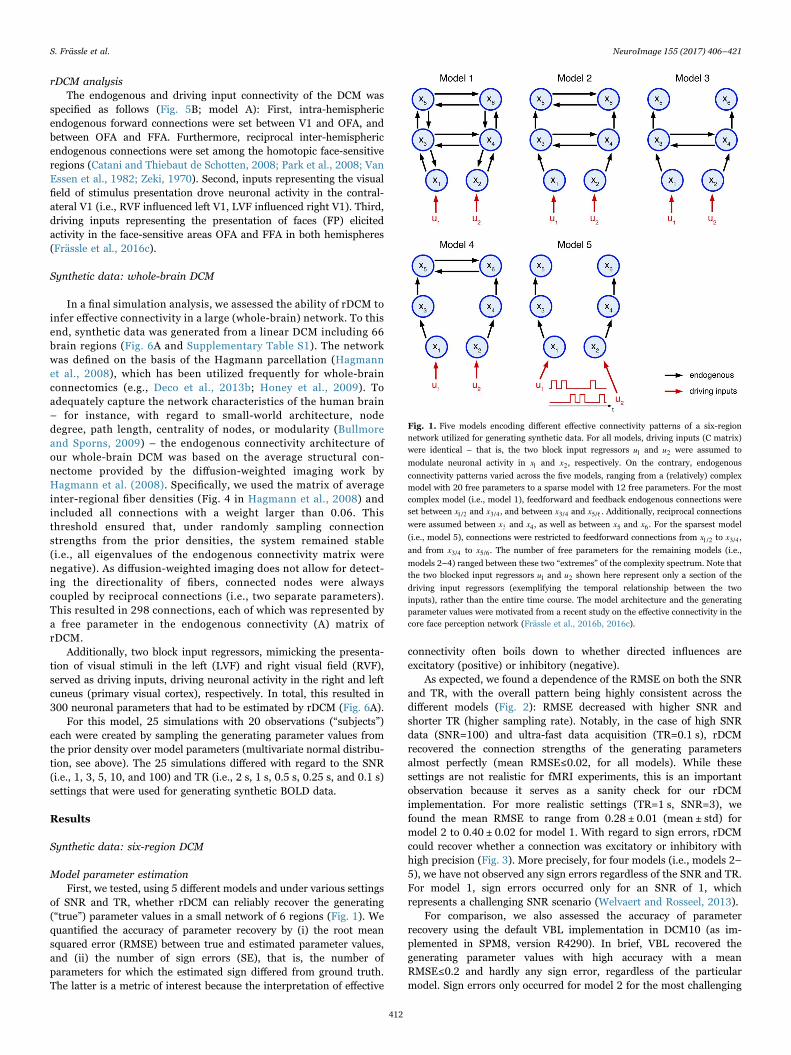
We assessed the face validity of rDCM in systematic simulationstudies, generating synthetic data for which the ground truth (i.e., thenetwork architecture and parameter values) was known. More pre-cisely, we generated data from 5 synthetic linear DCMs with identicaldriving inputs but distinct endogenous connectivity architectures(Fig. 1). For all models, two block input regressors u1 and u2 servedas driving inputs and were specified to elicit activity in x1 and x2,respectively. Each activation block lasted 14.5 s and alternated withbaseline periods of the same length.

While driving inputs were kept identical across models, varying theendogenous connectivity patterns yielded models of different complexity,with the most complex model consisting of 20 parameters (model 1) andthe sparsest model of 12 parameters (model 5). Specifically, for model 1,feedforward and feedback endogenous connections were set between x1/2and x3/4, and between x3/4 and x5/6. Additionally, reciprocal connectionswere assumed between x3 and x4, as well as between x5 and x6. Model 2

resulted from model 1 by discarding feedback connections, model 3 and 4from further removing reciprocal connections either at the highest orintermediate hierarchical level, respectively, and model 5 by consideringonly feedforward connections from x1/2 to x3/4, and from x3/4 to x5/6.

For each of these five models, 20 different sets of observations weregenerated. To ensure the data were realistic, we sampled the generating(“true”) parameter values of each simulation from the posteriordistributions of the endogenous and driving input parameters reportedin Frässle et al. (2016b). For each set of models and observations,synthetic BOLD data was then simulated under different conditionswhere we systematically varied the signal-to-noise ratio (SNR=[1, 3, 5,10, 100]) and repetition time (TR=[2 s, 1 s, 0.5 s, 0.25 s, 0.1 s]). Here,SNR was defined as the ratio between standard deviation of the signaland standard deviation of the noise (i.e., σ σSNR = /signal noise), where thenoise term is specified as additive white Gaussian noise with zeromean. This definition offers an intuitive measure of the ratio of thevariability of signal and noise, is a standard SNR measure in DCM andwell established for fMRI analyses more generally (Welvaert andRosseel, 2013). Under this definition, SNR levels of fMRI time seriesused for DCM are often 3 or higher; this is because these extracted timeseries result from a principal component analysis (over numerousvoxels in local volumes of interest) that suppresses noise. Evaluatingthe accuracy of parameter estimation and model selection under thedifferent settings of SNR and TR allowed us to assess the performanceof rDCM as a function of data quality and sampling rate, respectively(Figs. 2–4). Note that in all simulations of this initial paper, we used afixed (canonical) hemodynamic response function. In future work, wewill extend the model to account for variations in HRF over regions(see Discussion).

Empirical data: core face perception network

For application of rDCM to empirical fMRI data, we used apreviously published fMRI dataset from a simple face perceptionparadigm (the same dataset from which the generating parametervalues in the simulations above were sampled). A comprehensivedescription of the experimental design and data analysis can be foundelsewhere (Frässle et al., 2016b, 2016c); here, we only briefly summar-ize the most relevant information.

Participants and experimental designTwenty right-handed subjects viewed either gray-scale neutral faces (F),

objects (O), or scrambled (Fourier-randomized) images (S) in the left (LVF)or right visual field (RVF), while fixating a central cross (cf. Fig. 5A). Stimuliwere presented in a block design, with each block lasting 14.5 s duringwhich 36 stimuli of the same condition were shown (150 ms, ISI=250 ms).Subsequent stimulus blocks were interleaved with a resting period of thesame length where only the fixation cross was shown.

Data acquisition and analysisFor each subject, a total of 940 functional images were acquired on

a 3-T MR scanner (Siemens TIM Trio, Erlangen, Germany) using a T2*-

weighted single-shot gradient-echo echo-planar-imaging (EPI) se-quence (30 slices, TR=1450 ms, TE=25 ms, matrix size 64×64 voxels,voxel size 3×3×4 mm3, FoV=192×192 mm2, flip angle 90°). BOLDactivation patterns were analyzed using a first-level GLM (Friston et al.,1995) to identify brain regions sensitive to the processing of faces([2*F]-[O+S]), as well as to the visual field baseline contrasts (RVF,LVF). Six regions of interest (ROIs) were selected, representingoccipital face area (OFA; Puce et al., 1996), fusiform face area (FFA;Kanwisher et al., 1997), and primary visual cortex (V1), each in bothhemispheres (Fig. 5A). Peak coordinates of the ROIs were identified foreach subject individually (to account for inter-subject variability in theexact locations). From the individual ROIs, time series were extracted(removing signal mean and correcting for head movements), whichthen entered rDCM analyses.

S. Frässle et al. NeuroImage 155 (2017) 406–421

411

rDCM analysisThe endogenous and driving input connectivity of the DCM was

specified as follows (Fig. 5B; model A): First, intra-hemisphericendogenous forward connections were set between V1 and OFA, andbetween OFA and FFA. Furthermore, reciprocal inter-hemisphericendogenous connections were set among the homotopic face-sensitiveregions (Catani and Thiebaut de Schotten, 2008; Park et al., 2008; VanEssen et al., 1982; Zeki, 1970). Second, inputs representing the visualfield of stimulus presentation drove neuronal activity in the contral-ateral V1 (i.e., RVF influenced left V1, LVF influenced right V1). Third,driving inputs representing the presentation of faces (FP) elicitedactivity in the face-sensitive areas OFA and FFA in both hemispheres(Frässle et al., 2016c).

Synthetic data: whole-brain DCM

In a final simulation analysis, we assessed the ability of rDCM toinfer effective connectivity in a large (whole-brain) network. To thisend, synthetic data was generated from a linear DCM including 66brain regions (Fig. 6A and Supplementary Table S1). The networkwas defined on the basis of the Hagmann parcellation (Hagmannet al., 2008), which has been utilized frequently for whole-brainconnectomics (e.g., Deco et al., 2013b; Honey et al., 2009). Toadequately capture the network characteristics of the human brain– for instance, with regard to small-world architecture, nodedegree, path length, centrality of nodes, or modularity (Bullmoreand Sporns, 2009) – the endogenous connectivity architecture ofour whole-brain DCM was based on the average structural con-nectome provided by the diffusion-weighted imaging work byHagmann et al. (2008). Specifically, we used the matrix of averageinter-regional fiber densities (Fig. 4 in Hagmann et al., 2008) andincluded all connections with a weight larger than 0.06. Thisthreshold ensured that, under randomly sampling connectionstrengths from the prior densities, the system remained stable(i.e., all eigenvalues of the endogenous connectivity matrix werenegative). As diffusion-weighted imaging does not allow for detect-ing the directionality of fibers, connected nodes were alwayscoupled by reciprocal connections (i.e., two separate parameters).This resulted in 298 connections, each of which was represented bya free parameter in the endogenous connectivity (A) matrix ofrDCM.

Additionally, two block input regressors, mimicking the presenta-tion of visual stimuli in the left (LVF) and right visual field (RVF),served as driving inputs, driving neuronal activity in the right and leftcuneus (primary visual cortex), respectively. In total, this resulted in300 neuronal parameters that had to be estimated by rDCM (Fig. 6A).

For this model, 25 simulations with 20 observations (“subjects”)each were created by sampling the generating parameter values fromthe prior density over model parameters (multivariate normal distribu-tion, see above). The 25 simulations differed with regard to the SNR(i.e., 1, 3, 5, 10, and 100) and TR (i.e., 2 s, 1 s, 0.5 s, 0.25 s, and 0.1 s)settings that were used for generating synthetic BOLD data.

Results

Synthetic data: six-region DCM

Model parameter estimationFirst, we tested, using 5 different models and under various settings

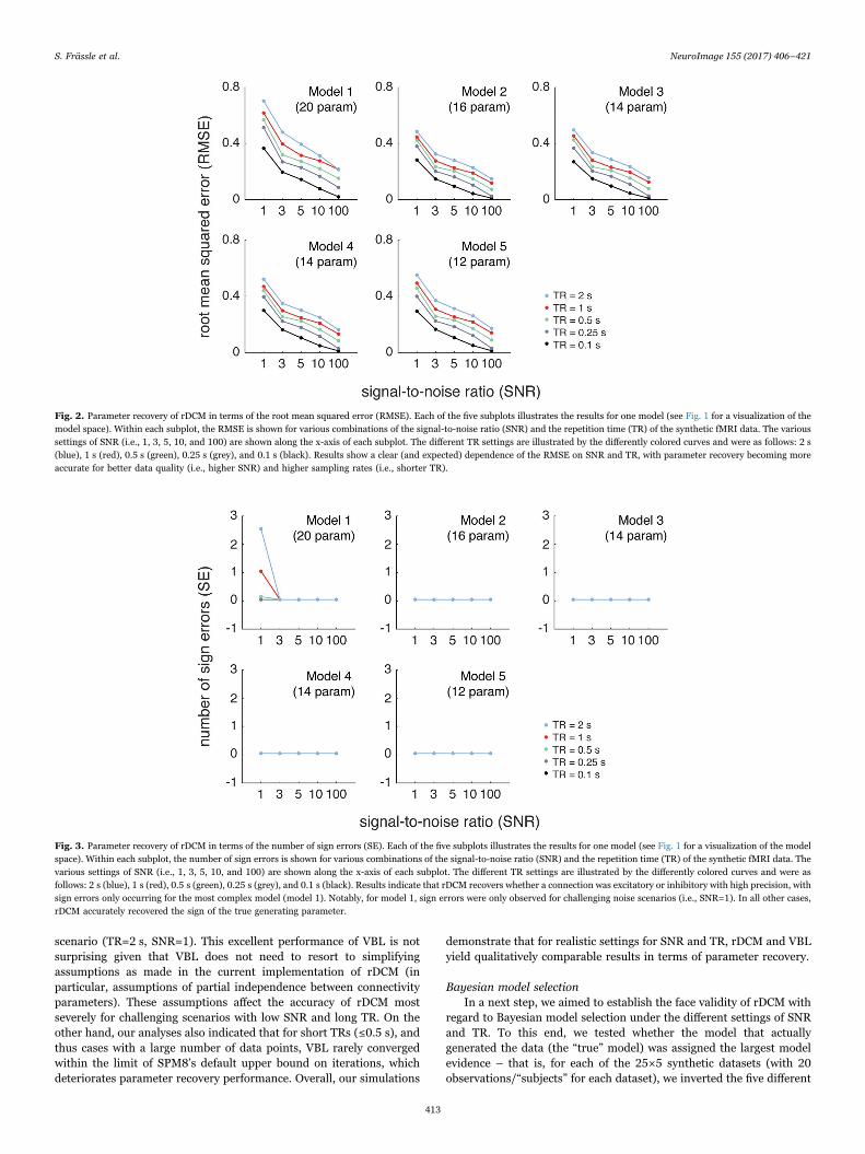
of SNR and TR, whether rDCM can reliably recover the generating(“true”) parameter values in a small network of 6 regions (Fig. 1). Wequantified the accuracy of parameter recovery by (i) the root meansquared error (RMSE) between true and estimated parameter values,and (ii) the number of sign errors (SE), that is, the number ofparameters for which the estimated sign differed from ground truth.The latter is a metric of interest because the interpretation of effective

connectivity often boils down to whether directed influences areexcitatory (positive) or inhibitory (negative).

As expected, we found a dependence of the RMSE on both the SNRand TR, with the overall pattern being highly consistent across thedifferent models (Fig. 2): RMSE decreased with higher SNR andshorter TR (higher sampling rate). Notably, in the case of high SNRdata (SNR=100) and ultra-fast data acquisition (TR=0.1 s), rDCMrecovered the connection strengths of the generating parametersalmost perfectly (mean RMSE≤0.02, for all models). While thesesettings are not realistic for fMRI experiments, this is an importantobservation because it serves as a sanity check for our rDCMimplementation. For more realistic settings (TR=1 s, SNR=3), wefound the mean RMSE to range from 0.28 ± 0.01 (mean ± std) formodel 2 to 0.40 ± 0.02 for model 1. With regard to sign errors, rDCMcould recover whether a connection was excitatory or inhibitory withhigh precision (Fig. 3). More precisely, for four models (i.e., models 2–5), we have not observed any sign errors regardless of the SNR and TR.For model 1, sign errors occurred only for an SNR of 1, whichrepresents a challenging SNR scenario (Welvaert and Rosseel, 2013).

For comparison, we also assessed the accuracy of parameterrecovery using the default VBL implementation in DCM10 (as im-plemented in SPM8, version R4290). In brief, VBL recovered thegenerating parameter values with high accuracy with a meanRMSE≤0.2 and hardly any sign error, regardless of the particularmodel. Sign errors only occurred for model 2 for the most challenging

Fig. 1. Five models encoding different effective connectivity patterns of a six-regionnetwork utilized for generating synthetic data. For all models, driving inputs (C matrix)were identical – that is, the two block input regressors u1 and u2 were assumed to

modulate neuronal activity in x1 and x2, respectively. On the contrary, endogenous

connectivity patterns varied across the five models, ranging from a (relatively) complexmodel with 20 free parameters to a sparse model with 12 free parameters. For the mostcomplex model (i.e., model 1), feedforward and feedback endogenous connections wereset between x1/2 and x3/4, and between x3/4 and x5/6. Additionally, reciprocal connections

were assumed between x3 and x4, as well as between x5 and x6. For the sparsest model

(i.e., model 5), connections were restricted to feedforward connections from x1/2 to x3/4,

and from x3/4 to x5/6. The number of free parameters for the remaining models (i.e.,

models 2–4) ranged between these two “extremes” of the complexity spectrum. Note thatthe two blocked input regressors u1 and u2 shown here represent only a section of the

driving input regressors (exemplifying the temporal relationship between the twoinputs), rather than the entire time course. The model architecture and the generatingparameter values were motivated from a recent study on the effective connectivity in thecore face perception network (Frässle et al., 2016b, 2016c).

S. Frässle et al. NeuroImage 155 (2017) 406–421

412

scenario (TR=2 s, SNR=1). This excellent performance of VBL is notsurprising given that VBL does not need to resort to simplifyingassumptions as made in the current implementation of rDCM (inparticular, assumptions of partial independence between connectivityparameters). These assumptions affect the accuracy of rDCM mostseverely for challenging scenarios with low SNR and long TR. On theother hand, our analyses also indicated that for short TRs (≤0.5 s), andthus cases with a large number of data points, VBL rarely convergedwithin the limit of SPM8’s default upper bound on iterations, whichdeteriorates parameter recovery performance. Overall, our simulations

demonstrate that for realistic settings for SNR and TR, rDCM and VBLyield qualitatively comparable results in terms of parameter recovery.

Bayesian model selectionIn a next step, we aimed to establish the face validity of rDCM with

regard to Bayesian model selection under the different settings of SNRand TR. To this end, we tested whether the model that actuallygenerated the data (the “true” model) was assigned the largest modelevidence – that is, for each of the 25×5 synthetic datasets (with 20observations/“subjects” for each dataset), we inverted the five different

Fig. 3. Parameter recovery of rDCM in terms of the number of sign errors (SE). Each of the five subplots illustrates the results for one model (see Fig. 1 for a visualization of the modelspace). Within each subplot, the number of sign errors is shown for various combinations of the signal-to-noise ratio (SNR) and the repetition time (TR) of the synthetic fMRI data. Thevarious settings of SNR (i.e., 1, 3, 5, 10, and 100) are shown along the x-axis of each subplot. The different TR settings are illustrated by the differently colored curves and were asfollows: 2 s (blue), 1 s (red), 0.5 s (green), 0.25 s (grey), and 0.1 s (black). Results indicate that rDCM recovers whether a connection was excitatory or inhibitory with high precision, withsign errors only occurring for the most complex model (model 1). Notably, for model 1, sign errors were only observed for challenging noise scenarios (i.e., SNR=1). In all other cases,rDCM accurately recovered the sign of the true generating parameter.

Fig. 2. Parameter recovery of rDCM in terms of the root mean squared error (RMSE). Each of the five subplots illustrates the results for one model (see Fig. 1 for a visualization of themodel space). Within each subplot, the RMSE is shown for various combinations of the signal-to-noise ratio (SNR) and the repetition time (TR) of the synthetic fMRI data. The varioussettings of SNR (i.e., 1, 3, 5, 10, and 100) are shown along the x-axis of each subplot. The different TR settings are illustrated by the differently colored curves and were as follows: 2 s(blue), 1 s (red), 0.5 s (green), 0.25 s (grey), and 0.1 s (black). Results show a clear (and expected) dependence of the RMSE on SNR and TR, with parameter recovery becoming moreaccurate for better data quality (i.e., higher SNR) and higher sampling rates (i.e., shorter TR).

S. Frässle et al. NeuroImage 155 (2017) 406–421

413

DCMs and compared the negative free energies by means of fixedeffects BMS (Stephan et al., 2009a). To this end, we computed theposterior model probability of the estimated model (Fig. 4). Notably, torule out that any of our BMS results were confounded by outliers(against which fixed effects analyses are vulnerable), we additionallycompared negative free energies by means of random effects BMS(Stephan et al., 2009a; as implemented in SPM12, version: R6685) andfound highly consistent results (data not shown).

As above, we observed the expected dependence of model selectionperformance on SNR and sampling rate. Specifically, model selectionbecame more accurate for higher SNR and shorter TR. For challengingscenarios with low signal-to-noise ratios (i.e., SNR=1), rDCM fre-quently failed to identify the correct model, except for extremely fastdata acquisitions (TR=0.1 s) where we find perfect recovery of the data-generating model architecture (Fig. 4, top row). More specifically, inthe case of noisy data, rDCM showed a tendency to selecting thesimplest of all models in our model space (Model 5) for TR≥0.5 s. This“Bayesian illusion” – where a simpler model, nested in a more complexdata-generating model, has higher evidence – is not an infrequentfinding when dealing with nested models that are only distinguished byparameters with weak effects or strongly correlated parameters, whoseeffects become difficult to detect in the presence of noise.

Having said this, given a reasonably high signal-to-noise ratio in thesynthetic fMRI data (i.e., SNR≥3), rDCM recovered the true model inthe vast majority of cases with hardly any model selection error (Fig. 4,rows 2–5). Even for relatively slow data acquisitions (TR=2 s), therewas only one case for which a “wrong” model had higher modelevidence compared to the generating (“true”) model. More specifically,in the case of model 1 being the “true” model, rDCM falsely assignedhighest evidence to model 2, suggesting that the presence of feedbackconnections can sometimes be difficult to detect – a finding which hasbeen highlighted previously (Daunizeau et al., 2011b).

Again, we compared rDCM to VBL by assessing model selectionperformance for the default implementation of DCM10. As expected,VBL recovered the true model perfectly with no model selection error.Consistent with our observations on parameter recovery reportedabove, differences between rDCM and VBL were thus only observedfor challenging scenarios (SNR=1), where the limitations of the currentversion of rDCM are likely to become most severe. On the contrary,both rDCM and VBL provide accurate model selection results forrealistic SNR and TR settings.

Computational burdenTo illustrate the computational efficiency of rDCM, we compared

run-times for rDCM with the time required to perform the respectivemodel inversion using the default VBL implementation in DCM10 (asimplemented in SPM8, version R4290). Specifically, we evaluated therun-times for all different settings of TR, under a fixed SNR of 3because we expected SNR to exert a smaller impact on run-times ascompared to TR, which essentially determines the number of datapoints. Our run-time results should be interpreted in a comparative,not absolute, manner, given their dependency on computer hardware.

Generally, model inversion under rDCM was considerably fasterthan VBL across all TR values (Table 1). For instance, for TR=1 s,rDCM was on average four orders of magnitude faster than VBL.Additionally, our analyses suggested that the computational efficiencyand feasibility of VBL-based DCM for large numbers of data points (aswould also be the case for DCMs with many regions) rapidlydiminishes. This behavior was not only reflected by the long run-timesreported in Table 1, which ranged from approximately 1,000–40,000 sper model inversion, but also (as mentioned above) by the fact that forshort TRs (and hence many data points), the VBL algorithm rarelyconverged within the limit of SPM8’s default upper bound on iterations(see the results for TR≤0.5 s in Table 1).

By comparison, rDCM handles large amounts of data more grace-fully due to the algebraic form of the likelihood function. In rDCM,model inversion took less than half a second, with no significantincrease in computation time when increasing the number of datapoints. This highlights the computational efficiency of rDCM and pointstowards its suitability for studying effective connectivity in very largenetworks, a theme we return to below.

It should be noted that in our comparative evaluation of rDCM andVBL, there is an additional computational saving under rDCM’s fixedform assumptions for the HRF. In other words, conventional DCMoptimizes the parameters of the hemodynamic response functionseparately for each region. This means that the number of parameters– that determines the number of solutions or integrations required toestimate free energy gradients – increases linearly for hemodynamicparameters and quadratically for neuronal (connectivity) parameters.This means that the VBL analyses could be made more efficient byadopting the rDCM (fixed form) assumptions for the HRF; however,the computational savings would not be very marked because the key(quadratic) determinant of computation time depends upon thenumber of connections.

Empirical data: core face perception network

Model parameter estimationWe applied rDCM to an empirical fMRI dataset of a simple face

perception task, which had been used previously to investigate intra-and inter-hemispheric integration in the core face perception network(Frässle et al., 2016a, 2016b, 2016c). Individual connectivity para-meters were estimated using model A (Fig. 5B, top), which thenentered summary statistics at the group level (one-sample t-tests,Bonferroni-corrected for multiple comparisons). We found all para-meter estimates to be excitatory except for the inhibitory self-connec-tions (Fig. 5C, left). Specifically, we found excitatory driving influencesof visual stimuli (LVF and RVF) on activity in right and left V1,

Fig. 4. Accuracy of Bayesian model comparison for rDCM. Each subplot illustrates themodel comparison results for a specific combination of the signal-to-noise ratio (SNR)and the repetition time (TR) of the synthetic fMRI data. The various settings of TR (i.e.,2 s, 1 s, 0.5 s, 0.25 s, and 0.1 s) are shown along the x-axis and the different SNR settings(i.e., 1, 3, 5, 10, and 100) are shown along the y-axis. For each combination of TR andSNR (i.e., each subplot), a matrix is shown that summarizes the fixed effects Bayesianmodel selection results for each of the five different models (see Fig. 1 for a visualizationof the model space). Specifically, each row in these matrices represents the posteriormodel probabilities of all DCMs that were used for model inversion (estimated) of theDCM that was used to actually generate the synthetic fMRI data (true). Specifically, eachrow signals whether rDCM was able to recover the true data-generating modelarchitecture among the five competing alternatives. Hence, a diagonal structure (i.e.,highest posterior probability on the diagonal) indicates that rDCM was able to recoverthe model that actually generated the data. Note that higher posterior probabilities arecolor-coded in warm colors (yellowish).

S. Frässle et al. NeuroImage 155 (2017) 406–421

414

respectively. Additionally, and in line with the well-established role ofbilateral OFA and FFA in face processing, we found excitatory face-specific driving influences on activity in all four regions of the core faceperception network. With regard to the endogenous connectivity, wefound excitatory connections both within each hemisphere and be-tween homotopic face-sensitive regions in both hemispheres, suggest-ing inter-hemispheric integration within the core face perceptionnetwork – in line with previous observations from functional(Davies-Thompson and Andrews, 2012) and effective connectivitystudies (Frässle et al., 2016c).

In an additional analysis step, we assessed the effective connectivity

in the same model (i.e., model A) using DCM10 (as implemented inSPM8, version R4290) in order to compare results from rDCM andVBL qualitatively. Note that a quantitative match of parameterestimates by rDCM and VBL cannot be expected since the generativemodels of these two frameworks are quite different. Three majordifferences are worth reiterating: First, while the hemodynamic modelin classical DCM is nonlinear and contains region-specific parameters,rDCM models the hemodynamic response as a fixed, linear convolutionof neuronal states. Second, rDCM uses a mean field approximation (orpartial independence assumption) that ignores potential dependenciesamongst parameters affecting different regions. Third, in contrast to

Fig. 5. Effective connectivity in the core face perception network as assessed with rDCM for an empirical fMRI dataset. (A) BOLD activation pattern shows regions that were moreactivated during the perception of faces as compared to objects and scrambled images, as determined by the linear face-sensitive contrast: [2*F]-[O+S]. Reproduced, with permission,from Frässle et al. (2016b) (top), as well as regions that were activated when stimuli were presented in the right (bottom, left) or left visual field (bottom, right). Results are thresholdedat a voxel-level threshold of p < 0.05 (FWE-corrected). (B) Two alternative models for explaining effective connectivity in the core face perception network. Both models assumed thesame endogenous connectivity (A matrix) – that is, intra-hemispheric feedforward connections from V1 to OFA and from OFA to FFA in both hemispheres, as well as reciprocal inter-hemispheric connections among the face-sensitive homotopic regions. Additionally, both models assumed driving inputs (C matrix) to the four face-sensitive regions (i.e., OFA and FFA,each in both hemispheres) by the processing of faces (FP). Critically, model A (top) and model B (bottom) differed in their driving inputs to left and right V1. While model A wasbiologically plausible by assuming that stimuli in the left (LVF) and right visual field (RVF) modulated activity in the contralateral V1, model B assumed these driving inputs to beswapped. (C) Group level parameter estimates for the endogenous and driving input connectivity of model A as estimated using rDCM (left) and VBL (right). Results are remarkablyconsistent across the two methods. The strength of each connection is displayed in terms of the mean coupling parameter (in [Hz]). Significant (p < 0.05, Bonferroni-corrected)connections are shown in full color; connections significant at an uncorrected threshold (p < 0.05) are shown in faded colors. L=left hemisphere; R=right hemisphere; A=anterior;P=posterior; LVF=left visual field; RVF=right visual field.

S. Frässle et al. NeuroImage 155 (2017) 406–421

415

the log-normal prior on noise variance in classical DCM, rDCM uses aGamma prior on noise precision. These differences in likelihoodfunctions and priors between rDCM and VBL translate into quantita-tively different posterior estimates (see Eq. (15)).

Qualitatively, however, parameter estimates by VBL were verysimilar to rDCM (Fig. 5C, right). In brief, all six driving inputs wereexcitatory (although this was not significant for the face-specific drivinginput to left FFA when correcting for multiple comparisons). Similarly,the intra-hemispheric forward connections in both hemispheres andthe inter-hemispheric connections among bilateral OFA were excita-

tory. One difference between VBL and rDCM parameter estimatesconcerned the inter-hemispheric connections among bilateral FFA,which were inhibitory for VBL. These inhibitory effects, however, didnot reach significance for the connection from right to left FFA (t(19)=-1.43, p=0.17), and only at an uncorrected statistical threshold for theconnection from left to right FFA (t(19)=-2.79, p=0.01).

Bayesian model selectionIn order to evaluate the Bayesian model selection (BMS) perfor-

mance of rDCM in an empirical setting, we constructed a second model

Table 1Computational burden of rDCM and VBL quantified in terms of the approximate run-times (in s) required for estimating a single linear DCM (i.e., model 1–5, here labelled as m1–m5,respectively) under various settings of the repetition time (TR) of the synthetic fMRI data. Note that run-times are reported exemplarily for a realistic signal-to-noise ratio (SNR) of 3.Run-times are given as the mean ± standard deviation of the 20 simulations, as well as the range.

Computational burden (s)

TR=2 s TR=1 s TR=0.5 s TR=0.25 s TR=0.1 s

Mean ± std Range Mean ± std Range Mean ± std Range Mean ± std Range Mean ± std Range

rDCM m1 0.20 ± 0.12 0.14–0.72 0.20 ± 0.12 0.14–0.69 0.23 ± 0.13 0.17–0.79 0.24 ± 0.12 0.19–0.74 0.37 ± 0.41 0.26–2.10m2 0.18 ± 0.11 0.13–0.63 0.19 ± 0.10 0.14–0.62 0.21 ± 0.12 0.15–0.72 0.26 ± 0.12 0.20–0.78 0.37 ± 0.37 0.26–1.94m3 0.16 ± 0.11 0.11–0.62 0.16 ± 0.09 0.12–0.53 0.18 ± 0.11 0.13–0.62 0.20 ± 0.10 0.15–0.62 0.33 ± 0.32 0.23–1.70m4 0.18 ± 0.11 0.12–0.62 0.19 ± 0.10 0.14–0.61 0.21 ± 0.12 0.15–0.74 0.27 ± 0.14 0.20–0.85 0.37 ± 0.38 0.26–1.98m5 0.19 ± 0.11 0.12–0.67 0.20 ± 0.11 0.15–0.68 0.23 ± 0.14 0.17–0.82 0.27 ± 0.13 0.20–0.81 0.38 ± 0.40 0.26–2.08

VBL m1 1157 ± 477 830–2498 3589 ± 1153 2432–5448 7932 ± 1169 6303–9986 17704 ± 1124 16484–19143 43633 ± 3904 40449–51119m2 1970 ± 563 893–2452 3566 ± 597 2380–4048 7811 ± 939 6859–10349 14804 ± 760 14229–16357 37322 ± 2367 35248–41464m3 1592 ± 436 1075–2294 3497 ± 567 2507–4209 7228 ± 444 6715–7935 13741 ± 801 13198–16924 35738 ± 3265 32106–43923m4 1177 ± 277 987–2283 2649 ± 469 2214–4295 6654 ± 693 5946–8289 14301 ± 1265 13387–18147 33791 ± 1838 32455–37599m5 819 ± 55 733–920 2166 ± 161 1930–2574 5725 ± 560 5217–7184 13691 ± 1165 12422–15907 32014 ± 1934 30354–35322

Fig. 6. Parameter recovery of rDCM in terms of the root mean squared error (RMSE) and the number of sign errors (SE) for the large (whole-brain) network. (A) Endogenousconnectivity architecture (A matrix) among the 66 brain regions from the Hagmann parcellation. Endogenous connectivity was restricted to the most pronounced edges of the humanstructural connectome by only selecting those connections for which an average inter-regional fiber density larger than 0.06 has been reported in Hagmann et al. (2008). Additionally,two block input regressors u1 and u2, mimicking the effect of visual stimulation in the right and the left visual field, were assumed to modulate neuronal activity in left and right cuneus

(primary visual cortex), respectively. The brain network was visualized with the BrainNet Viewer (Xia et al., 2013), which is available as open-source software for download (http://www.nitrc.org/projects/bnv/) (left). An actual “observation” of the endogenous connectivity, generated by sampling connection strengths from the prior density on the endogenousparameters (right). A complete list of the anatomical labels of the 66 parcels can be found in the Supplementary Table S1. (B) The RMSE and (C) the number of sign errors are shownfor various combinations of the signal-to-noise ratio (SNR) and the repetition time (TR) of the synthetic fMRI data. The various settings of SNR (i.e., 1, 3, 5, 10, and 100) are shownalong the x-axis of each subplot. The different TR settings are illustrated by the differently colored curves and were as follows: 2 s (blue), 1 s (red), 0.5 s (green), 0.25 s (grey), and 0.1 s(black). (D) Number of sign errors (SE) for the different SNR and TR settings when restricting the analysis to parameter estimates that showed a non-negligible effect size (i.e., the 95%Bayesian credible interval of the posterior not containing zero). For these parameters, the number of SE was considerably reduced, suggesting that the sign of an endogenous influences(i.e., inhibitory vs. excitatory) could be adequately recovered for parameters of large effect size. L=left hemisphere; R=right hemisphere; A=anterior; P=posterior; LVF=left visual field;RVF=right visual field.

S. Frässle et al. NeuroImage 155 (2017) 406–421

416

(model B; Fig. 5B, bottom) and inverted this model under rDCM andVBL, respectively. Importantly, in this alternative model, the visualbaseline driving inputs were permuted compared to the original model(model A). In contradiction to neuroanatomy, model B thus proposedthat visual stimuli presented in the periphery entered ipsilateral V1(i.e., LVF influenced left V1, RVF influenced right V1). Hence, weexpected both rDCM and VBL to select model A as the winning model.

We used random effects BMS (Stephan et al., 2009a; as implemen-ted in SPM12, version: R6685) to compare the two alternative modelsbased on their negative free energies. For both, rDCM and VBL, modelA was the decisive winning model with a protected exceedanceprobability of 1.00 in either case (Rigoux et al., 2014). This indicatesthat rDCM not only yields BMS results comparable to VBL (withequally high confidence), but also selects the expected and biologicallymore plausible model amongst two competing hypotheses.

Computational burdenWe evaluated the run-time of rDCM and VBL for both models A and

B. Again, we would like to highlight that the reported values should beinterpreted in a comparative, not absolute, manner as they depend onthe specific hardware and software settings. Consistent with ourprevious observations in the context of simulations, we found modelinversion under rDCM to be on average three orders of magnitudefaster than VBL (Table 2). More precisely, rDCM was highly efficienttaking less than half a second per model, whereas the time required formodel inversion under VBL was on the order of 15 min.

Regression DCM for large-scale networks

Model parameter estimationIn a final step, we used simulations to evaluate the utility of rDCM

for inferring effective connectivity in a large (whole-brain) network. Wechose a network comprising 66 brain regions and 300 free connectivityparameters (Fig. 6A), where model structure was based on thestructural connectome provided by the diffusion-weighted imagingwork by Hagmann et al. (2008). As above, we computed the root meansquared error (RMSE) and the number of sign errors (SE) to quantifythe accuracy of parameter recovery.

Consistent with our previous findings from the synthetic andempirical dataset, we observed a dependence of both the RMSE andSE on SNR and TR, indicating that parameter estimation improvedwith increasing data quality (i.e., higher SNR) and sampling rates (i.e.,shorter TR). For a realistic setting of fMRI data (TR=1 s, SNR=3), theRMSE was 0.29 ± 0.01 (Fig. 6B). In the case of high SNR data(SNR=100) and ultra-fast data acquisition (TR=0.1 s), the RMSE was0.09 ± 0.02. While the RMSE for this case of “ideal data” is larger thanin the simulations using the much smaller six-region network above,errors are still in an acceptable range, indicating a promising scalabilityof rDCM.

It is worth highlighting that even for “ideal data”, one would notexpect rDCM (nor VBL or any other model inversion method) to exactly

recover the “true” parameter values that were used to simulate the data.This is because Bayesian methods optimize the posterior rather thanthe likelihood, and the influence of the prior exerts a bias on modelparameter recovery whenever the prior mean does not coincide exactlywith the parameter values used for data generation. This can producecounterintuitive results: even when both prior and likelihood havemeans of the same sign, parameter dependencies (which arise from themathematical form of the likelihood function) can lead to a posteriormean of the opposite sign (see Supplementary Fig. S1 for a graphicalvisualization). For pronounced parameter interdependencies (whichare unavoidable in large-scale models with hundreds of free para-meters), this sign flipping can occur even when prior mean and datamean (likelihood) are identical, provided their means are not too faraway from zero.

Given these considerations, it was unsurprising to find that rDCMof the whole-brain model suffered from considerably more sign errorsthan the small six-region DCMs described above (Fig. 6C). Again, thiswas a function of SNR and TR: While only 4.0 ± 1.9 sign errorsoccurred for high quality data (TR=0.1 s, SNR=100), we observed45.7 ± 4.6 sign errors in more realistic settings (TR=1 s, SNR=3),corresponding to an error rate of 15.2 ± 1.5%.

As illustrated by Supplementary Fig. S1, the likelihood of signflipping having occurred is smaller for parameters whose posteriormean deviates strongly from zero. In a second analysis, we thereforerestricted the evaluation of the sign errors to those connections forwhich zero was not within the 95% Bayesian credible interval of theposterior density. In this way, we asked whether estimates of connec-tions that provided sufficiently large evidence for an effect could betrusted (in terms of revealing the correct direction of influence). Whenfocusing on these connections, sign errors were considerably reduced(Fig. 6D). Specifically, even for (relatively) slow image acquisitions andnoisy data (TR=2 s; SNR=1), the number of sign errors was in anacceptable range (19.5 ± 5.1, corresponding to an error rate of 6.5 ±1.7%). For more realistic image acquisition and SNR settings (TR=1 s;SNR=3), the number of sign errors reduced to 12.4 ± 3.3 (error rate of4.1 ± 1.1%). Ultimately, when approaching ideal data (TR=0.1 s;SNR=100), hardly any sign error was observed (2.2 ± 1.1, correspond-ing to an error rate of 0.7 ± 0.4%). This suggests that parameterestimates representing a non-trivial effect size (i.e., the 95% Bayesiancredible interval not containing zero) correctly indicate the direction ofinfluences, rendering rDCM a meaningful tool for inferring effectiveconnectivity patterns in large (whole-brain) networks.

Computational burdenWe evaluated the run-time of rDCM for the whole-brain DCM for

all possible combinations of SNR and TR. Again, the reported valuesshould be interpreted in a qualitative, not absolute, manner as theydepend on the specific hardware and software settings. We foundmodel inversion to be extremely efficient even for such a large numberof brain regions and free parameters. More specifically, estimation ofthe model using rDCM took on average 2–3 s (Table 3), suggesting thatour approach scales easily with the number of brain regions (datapoints) and, thus, makes inference on the effective connectivity in large(whole-brain) networks computationally feasible.

Discussion

In this paper, we have introduced regression DCM (rDCM) forfunctional magnetic resonance imaging (fMRI) data as a novel variantof DCM that enables computationally highly efficient analyses ofeffective connectivity in large-scale brain networks. This developmentrests on reformulating a linear DCM in the time domain as a specialcase of Bayesian linear regression (Bishop, 2006) in the frequencydomain, together with a highly efficient VB inference scheme. Usingsynthetic and empirical data, we first demonstrated the face validity ofrDCM for small six-region networks before providing a simulation-

Table 2Computational burden of rDCM and VBL quantified in terms of the approximate run-times (in s) required for estimating a single linear DCM (i.e., model A or model B) of theintra- and inter-hemispheric connectivity in the core face perception network. The run-times required for inverting the model are given as the mean ± standard deviation of the20 subjects, as well as the range.

Computational burden (s)

Mean ± std Range

rDCM Model A 0.24 ± 0.03 0.21–0.28Model B 0.26 ± 0.04 0.21–0.32

VBL Model A 827.3 ± 233.4 519.7–1422.2Model B 973.3 ± 371.7 491.6–1706.3

S. Frässle et al. NeuroImage 155 (2017) 406–421

417

based proof-of-principle for using rDCM to infer effective connectivityin a large network consisting of 66 brain regions, with a realistic humanstructural connectome and 300 free parameters to be estimated.

Our initial simulations using a six-region network (a typical size ofconventional DCMs) indicated that, as expected, the accuracy of rDCM– with regard to both parameter estimation and model comparison –varies as a function of the signal-to-noise ratio (SNR) and therepetition time (TR) of fMRI data. Overall, our results demonstratedreasonable performance with regard to parameter recovery and modelselection accuracy but also highlighted the importance of sufficientlyhigh SNR (3 or higher) and fast data acquisition (TR < 2 s) for veridicalinference. In situations where these conditions are not met (e.g., forsubcortical regions with inherently low SNR), the current formulationof rDCM might not give reliable results. Our simulations suggest thatthe early version of rDCM reported in this paper is particularlypromising when exploiting sophisticated scanner hardware and/oracquisition sequences that boost SNR and reduce TR. Fortunately,the development trends in fMRI move in the required direction. Forexample, high-field MRI (7 T and beyond) allows for considerablyhigher SNRs (Duyn, 2012; Redpath, 1998) and 7 T MR scanners arenow becoming widely available. Similarly, the application of ultra-fastinverse imaging and multiband EPI techniques enable very highsampling rates (with TRs far below one second) with whole-braincoverage (Lin et al., 2012; Moeller et al., 2010; Xu et al., 2013).Alternatively, even conventional data acquisition focused on regions ofinterest and using only a few slices enables TRs with only a fewhundred milliseconds (for a previous DCM example, see Kasess et al.,2008). Taking advantage of such methodological advancements mayhelp to further exploit the full potential of rDCM for inferring effectiveconnectivity from fMRI data. However, whether the benefits of shortTRs for rDCM translate from simulations to real world datasets needsto be examined by empirical validation studies; for example, by testingwhether the accuracy of connectivity-based decoding of diagnosticstatus (cf. Brodersen et al., 2011) is improved by short TRs.

Having established the validity of rDCM for six-region networks, wethen provided a proof-of-principle that rDCM is suitable for inferringeffective connectivity in a whole-brain network comprising 66 nodes, withconnectivity according to the human structural connectome reported inHagmann et al. (2008) and 300 free parameters to estimate. These analysessuggested that rDCM can adequately recover connectivity parameters inlarge networks whose size is an order of magnitude larger than currentlyestablished DCM applications. Importantly, our run-time analyses suggest,that the approach scales easily and can be applied to much larger networks,provided that enough data are available. Specifically, run-time analyses didnot indicate a significant increase in computation time when increasing thenumber of data points. Even for the shortest TR, corresponding to roughly13,500 data points (per brain region), run-time was still only on the orderof 2–3 s. The striking efficiency of rDCM rests on the fact that – due to thealgebraic form of the likelihood function in the frequency domain – thecomputationally most expensive operation on each iteration is essentiallythe inversion of an N×N covariance matrix (whereas, in VBL, it is the

computation of an N×N Hessian, in addition to integrating the stateequation).

These findings suggest that rDCM has promising potential for theexploration of effective connectivity patterns in large (whole-brain)networks. We presently see four main application domains. First, giventhe computational efficiency of rDCM – which only requires fewseconds for the inversion of whole-brain DCMs including an estimateof the negative free energy as an approximation to the log modelevidence – it may serve as a useful tool for network discovery (Biswalet al., 2010; Friston et al., 2011). Second, it may enable the applicationof graph theoretical approaches to effective connectivity patterns fromlarge networks, which have so far been restricted to structural andfunctional connectivity (for a comprehensive review, see Bullmore andSporns, 2009; Rubinov and Sporns, 2010). Extending graph theory toeffective connectivity estimates in networks of non-trivial size opens upexciting new possibilities for studying the functional integration of thehuman brain. Specifically, given the inherently directed network of thehuman brain, graph-theoretical measure such as small-worldness,node degree, path length, centrality of nodes, or modularity will onlyprovide an accurate view on the network topology underlying braindynamics when accommodating the directionality of edges. Third,regardless of whether brain-wide effective connectivity estimates areused by themselves or undergo further (e.g., graph-theoretical) proces-sing, rDCMmay serve useful for computational phenotyping of patientswith diseases for which global dysconnectivity is suspected, such asschizophrenia (Bullmore et al., 1997; Friston and Frith, 1995;Pettersson-Yeo et al., 2011; Stephan et al., 2006). Finally, due to itshigh computational efficiency, rDCM would be ideally suited forinitializing the starting values of the VBL algorithm for standardDCM analyses of effective connectivity. This could be achieved byrunning rDCM repeatedly from multiple starting points (either definedas a grid in parameter space or randomly chosen) and using the modelwith the highest evidence to provide a starting point for subsequentVBL under conventional DCM. This might not only considerably speedup model inversion under the current DCM framework but potentiallyalso prevent the algorithm from getting stuck in local extrema, againstwhich local optimization schemes like VBL are vulnerable (Daunizeauet al., 2011a).

So far, there has only been one study that extended DCM for fMRIto larger networks (Seghier and Friston, 2013). This approach usedfunctional connectivity measures to provide prior constraints thatbounded the effective number of free parameters by essentiallyreplacing the number of nodes with a (lower) number of modes (theprincipal components of the functional connectivity matrix). Seghierand Friston (2013) described their approach by an application to anetwork consisting of 20 regions, and it remains to be tested whetherthis approach also generalizes to a larger number of network nodes asrequired for whole-brain connectomics under commonly used parcella-tion schemes (e.g., Deco et al., 2013b; Hagmann et al., 2008; Honeyet al., 2009).

Investigating connectivity in large-scale networks by means of

Table 3Computational burden of rDCM quantified in terms of the approximate run-times (in s) required for estimating the large (whole-brain) DCM consisting of 66 brain regions, with arealistic human structural connectome and 300 free parameters. Run-times are shown for various combinations of the signal-to-noise ratio (SNR) and the repetition time (TR) of thesynthetic fMRI data. The run-times required for inverting the model are given as the mean ± standard deviation of the 20 simulations, as well as the range.

SNR Computational burden (s)

TR=2 s TR=1 s TR=0.5 s TR=0.25 s TR=0.1 s

Mean ± std Range Mean ± std Range Mean ± std Range Mean ± std Range Mean ± std Range

1 1.7 ± 0.3 1.2–2.3 1.8 ± 0.4 1.3–2.7 1.4 ± 0.2 1.1–1.7 1.8 ± 0.3 1.2–2.4 3.1 ± 0.2 2.8–3.43 1.6 ± 0.4 1.1–2.7 1.7 ± 0.6 1.2–3.1 1.4 ± 0.3 1.1–1.8 1.7 ± 0.3 1.4–2.4 3.2 ± 0.2 2.8–3.55 1.6 ± 0.4 1.2–2.8 1.8 ± 0.4 1.4–3.0 1.4 ± 0.2 1.1–1.9 1.8 ± 0.4 1.3–2.5 3.2 ± 0.2 2.9–3.710 1.7 ± 0.4 1.2–2.6 2.4 ± 0.3 1.9–3.0 1.5 ± 0.2 1.2–1.7 1.8 ± 0.3 1.3–2.4 3.0 ± 0.3 2.8–3.9100 1.8 ± 0.4 1.5–2.6 2.0 ± 0.3 1.5–2.9 1.5 ± 0.1 1.3–1.7 1.6 ± 0.2 1.3–2.0 3.2 ± 0.3 2.8–3.8

S. Frässle et al. NeuroImage 155 (2017) 406–421

418

mathematical models has been addressed from a different methodolo-gical angle using biophysical network models (BNM; Deco et al., 2013a,2013b; Honey et al., 2007, 2009; Sanz-Leon et al., 2015; Woolrich andStephan, 2013). BNMs of fMRI data typically consist of up to 103

network nodes, where each node is represented by a neural mass ormean-field model of local neuronal populations. Nodes are linked bylong-range connections which are typically based on anatomicalknowledge from human diffusion-weighted imaging data or from tracttracing studies in the macaque monkey. The resulting networkdynamics are then fed into an observation model to predict fMRI data.The complexity of BNMs, however, has so far prevented estimating thestrengths of individual connections. Existing applications have typicallyfocused on simulations under fixed parameters (Deco et al., 2013a;Honey et al., 2007) or used a simplified model allowing for theestimation of a global scaling parameter (Deco et al., 2013b).Critically, such a single parameter has an indiscriminative effect onall connections, which cannot capture the selective changes in subsetsof long-range connections evoked by cognitive processes. The ability ofrDCM to estimate the strengths of individual connections in large-scalenetworks may represent a starting point for further convergencebetween DCMs and BNMs, as has been predicted repeatedly in therecent past (Deco and Kringelbach, 2014; Stephan et al., 2015).

Notably, whole-brain connectivity analyses face a number ofpotential pitfalls and challenges, regardless whether structural, func-tional or effective connectivity measures are obtained (Fornito et al.,2013; Kelly et al., 2012). Among others, this includes the correctidentification of nodes and edges, the highly complex and dynamicstructure of noise in fMRI, and the development of rigorous statisticalframeworks for the analysis of whole-brain graphs. For instance,macroscopic criteria for parcellating the brain into functionally mean-ingful and biologically valid nodes are only just emerging (Glasseret al., 2016). Valid node identification is critical for accurate mappingof inter-regional connectivity (Smith et al., 2011) and ill-defined nodescan have profound impact on the inferred organization of the brain as,for instance, derived from graph-theoretical measures (Fornito et al.,2010). Similarly, statistical frameworks need to be refined to addresskey challenges in the analysis of whole-brain connectomes – includingthe multiple comparison problem, graph thresholding, and the inter-pretation of topological measures (Fornito et al., 2013). A systematicand thorough assessment of these issues will therefore be of majorimportance for whole-brain connectivity analyses in the near future.

We would like to emphasize that the current implementation ofrDCM only represents a starting point of development and is subject tothree major limitations when compared to the original DCM framework.First, due to the replacement of the hemodynamic forward model with afixed hemodynamic response function, rDCM does not presently capturethe variability in the BOLD signal across brain regions and individuals(Aguirre et al., 1998; Handwerker et al., 2004). Critically, accounting forthe inter-regional variability is crucial to avoid confounds when inferringeffective connectivity from fMRI data (David et al., 2008; Valdes-Sosaet al., 2011). In forthcoming work, we will improve rDCM by replacingthe fixed HRF with a basis set of hemodynamic response functions (i.e., acanonical HRF, and its temporal and dispersion derivatives; Fristonet al., 1998), which can capture variations in the latency and duration ofhemodynamic responses. This basis set is almost identical to theprincipal components of variation with respect to the hemodynamicmodel used in DCM, conferring biophysical validity to the set (Fristonet al., 2000). An alternative approach to account for inter-regionalvariability in hemodynamic responses would be to use a linearizedversion of the hemodynamic model in DCM as described in previouswork (Stephan et al., 2007).

Second, in its current implementation, rDCM ignores possibleinterdependencies between connections that affect different regions.This is because we assumed the measurement noise to be an indepen-dent random vector with noise precision τ and neglected its depen-dency on the endogenous connectivity parameters. We will improve

this approximation by introducing appropriate covariance components(similar to standard approaches to non-sphericity correction in con-ventional GLM analyses; Friston et al., 2002) and augment ourinference scheme to estimate these additional hyperparameters.

Third, rDCM is restricted to linear models (i.e., DCMs that includean A and C matrix) and thus cannot account for modulatory influencesby experimental manipulations (B matrix). A bilinear extension to therDCM approach is challenging in that the bilinear term of the neuronalstate equation in the time domain induces a convolution of theexperimental input and the noise term in the frequency domain. Thisleads to a non-trivial structure of the error covariance matrix.Addressing these three major limitations in forthcoming extensionswill further improve the utility of rDCM for inferring effectiveconnectivity among neuronal populations from fMRI data.

Apart from addressing the limitations mentioned above, there aretwo further important extensions that we will present in forthcomingwork. First, while the present model is designed to work withexperimentally controlled perturbations (the driving inputs in rDCM)and hence task-related fMRI, it is possible to extend the model todescribe the “resting state”, i.e., unconstrained cognition in the absenceof external pertubations. A second important advance concerns theintroduction of sparsity constraints to our approach (see Lomakina,2016). This sparse rDCM (srDCM; Frässle et al., in preparation) is oflikely importance for the analysis of large-scale networks – bothbecause a complete description of larger networks complicates inter-pretability, but also because the available measurements may not offersufficient information (i.e., number of data points per parameter) toallow for precise estimation of all connectivity parameters. Theformulation of rDCM as a linear regression problem makes thisextension of rDCM straightforward, as we can exploit well-establishedmethods for sparse linear regression and feature selection such asLASSO (Tibshirani, 1996), elastic net regularization (Zou and Hastie,2005), or Spike-and-Slab priors for Bayesian linear regression(Hernandez-Lobato et al., 2013). The ensuing automatic pruning ofconnections could be further informed by including information aboutthe strength or likelihood of anatomical connections (cf. anatomicallyinformed priors in DCM; Stephan et al., 2009b). These methods allimplement some form of sparsity hyperpriors on the parameters; eitherimplicitly or explicitly. An alternative to these bespoke models ofsparsity would be to use Bayesian model reduction (Friston et al.,2016) where parameters are removed (and thus connectivity graphs arereduced) using an efficient scoring of models. In our context, this mayrepresent an efficient alternative way to introduce sparsity – basedupon the posterior densities furnished by rDCM. In summary, aug-menting the current rDCM approach with the ability to impose sparsityconstraints may result in a powerful tool for automatic “pruning” ofwhole-brain graphs to the most essential connections.

Finally, we would like to emphasize that the analysis of effectiveconnectivity in whole-brain networks will not only prove valuable forstudying the neural basis of cognitive processes in the healthy humanbrain, but may also contribute to a deeper understanding of patho-physiology of psychiatric and neurological disorders. A translationalneuromodeling approach to neuroimaging data has potential forestablishing novel diagnostic and predictive tools, enabling the emer-gence of Computational Psychiatry and Computational Neurology(Deco and Kringelbach, 2014; Friston et al., 2014b; Huys et al.,2011; Maia and Frank, 2011; Montague et al., 2012; Stephan andMathys, 2014; Stephan et al., 2015). Here, one important goal concernsthe stratification of patients from heterogeneous spectrum diseasesinto mechanistically more well-defined subgroups that have predictivevalidity for individual treatment responses. Despite some encouragingfirst successes of insights into heterogeneous spectrum diseases basedon connectivity inferred from fMRI data (e.g., Anticevic et al., 2015;Brodersen et al., 2014; Dima et al., 2009; Yang et al., 2014),considerable challenges remain that have so far prevented the success-ful transition to clinical applications (Stephan et al., 2015). The

S. Frässle et al. NeuroImage 155 (2017) 406–421

419

computational approach introduced in this paper may serve useful inthis regard since rDCM represents a step towards a practical andcomputationally extremely efficient approach to obtaining directedestimates of individual connections in networks of non-trivial size,rendering computational phenotyping of whole-brain dynamics afeasible endeavour.

Software note

A MATLAB implementation of the rDCM approach introduced inthis paper will be made available as open source code in a future releaseof the TAPAS Toolbox (www.translationalneuromodeling.org/software).

Acknowledgements

We thank Jakob Heinzle and Lars Kasper for helpful advice. Thiswork was supported by the ETH Zurich Postdoctoral FellowshipProgram and the Marie Curie Actions for People COFUND Program(both to SF), as well as the René and Susanne Braginsky Foundationand the University of Zurich (KES).

Appendix A. Supplementary material

Supplementary data associated with this article can be found in theonline version at http://dx.doi.org/10.1016/j.neuroimage.2017.02.090.

References

Aguirre, G.K., Zarahn, E., D'esposito, M., 1998. The variability of human, BOLDhemodynamic responses. Neuroimage 8, 360–369.

Anticevic, A., Hu, X., Xiao, Y., Hu, J., Li, F., Bi, F., Cole, M.W., Savic, A., Yang, G.J.,Repovs, G., Murray, J.D., Wang, X.J., Huang, X., Lui, S., Krystal, J.H., Gong, Q.,2015. Early-course unmedicated schizophrenia patients exhibit elevated prefrontalconnectivity associated with longitudinal change. J. Neurosci. 35, 267–286.

Bishop, C.M., 2006. Pattern Recognition and Machine Learning. Springer, New York, 105, (12, 13, 47).

Biswal, B.B., Mennes, M., Zuo, X.N., Gohel, S., Kelly, C., Smith, S.M., Beckmann, C.F.,Adelstein, J.S., Buckner, R.L., Colcombe, S., Dogonowski, A.M., Ernst, M., Fair, D.,Hampson, M., Hoptman, M.J., Hyde, J.S., Kiviniemi, V.J., Kötter, R., Li, S.J., Lin,C.P., Lowe, M.J., Mackay, C., Madden, D.J., Madsen, K.H., Margulies, D.S., Mayberg,H.S., McMahon, K., Monk, C.S., Mostofsky, S.H., Nagel, B.J., Pekar, J.J., Peltier, S.J.,Petersen, S.E., Riedl, V., Rombouts, S.A., Rypma, B., Schlaggar, B.L., Schmidt, S.,Seidler, R.D., Siegle, G.J., Sorg, C., Teng, G.J., Veijola, J., Villringer, A., Walter, M.,Wang, L., Weng, X.C., Whitfield-Gabrieli, S., Williamson, P., Windischberger, C.,Zang, Y.F., Zhang, H.Y., Castellanos, F.X., Milham, M.P., 2010. Toward discoveryscience of human brain function. Proc. Natl. Acad. Sci. USA 107, 4734–4739.

Bracewell, R., 1999. The Fourier Transform and its Applications 3rd Edition. McGraw-Hill Science/Engineering/Math.

Brodersen, K.H., Schofield, T.M., Leff, A.P., Ong, C.S., Lomakina, E.I., Buhmann, J.M.,Stephan, K.E., 2011. Generative embedding for model-based classification of fMRIdata. PLoS Comput. Biol. 7, e1002079.

Brodersen, K.H., Deserno, L., Schlagenhauf, F., Lin, Z., Penny, W.D., Buhmann, J.M.,Stephan, K.E., 2014. Dissecting psychiatric spectrum disorders by generativeembedding. Neuroimage Clin. 4, 98–111.

Buckner, R.L., Krienen, F.M., Yeo, B.T., 2013. Opportunities and limitations of intrinsicfunctional connectivity MRI. Nat. Neurosci. 16, 832–837.

Bullmore, E.T., Sporns, O., 2009. Complex brain networks: graph theoretical analysis ofstructural and functional systems. Nat. Rev. Neurosci. 10, 186–198.

Bullmore, E.T., Frangou, S., Murray, R.M., 1997. The dysplastic net hypothesis: anintegration of developmental and dysconnectivity theories of schizophrenia.Schizophr. Res. 28, 143–156.

Buxton, R., Wong, E., Frank, L., 1998. Dynamics of blood flow and oxygenation changesduring brain activation: the balloon model. Magn. Reson. Med. 39, 855–864.

Catani, M., Thiebaut de Schotten, M., 2008. A diffusion tensor imaging tractography atlasfor virtual in vivo dissections. Cortex 44, 1105–1132.

Daunizeau, J., Friston, K., Kiebel, S., 2009. Variational Bayesian identification andprediction of stochastic nonlinear dynamic causal models. Physica D-NonlinearPhenom. 238, 2089–2118.

Daunizeau, J., David, O., Stephan, K., 2011a. Dynamic causal modelling: a critical reviewof the biophysical and statistical foundations. Neuroimage 58, 312–322.

Daunizeau, J., Preuschoff, K., Friston, K., Stephan, K., 2011b. Optimizing experimentaldesign for comparing models of brain function. PLoS Comput. Biol. 7.

David, O., Guillemain, I., Saillet, S., Reyt, S., Deransart, C., Segebarth, C., Depaulis, A.,2008. Identifying neural drivers with functional MRI: an electrophysiologicalvalidation. PLoS Biol. 6, 2683–2697.

Davies-Thompson, J., Andrews, T.J., 2012. Intra- and interhemispheric connectivity

between face-selective regions in the human brain. J. Neurophysiol. 108,3087–3095.

Deco, G., Kringelbach, M.L., 2014. Great expectations: using whole-brain computationalconnectomics for understanding neuropsychiatric disorders. Neuron 84, 892–905.

Deco, G., Jirsa, V.K., McIntosh, A.R., 2013a. Resting brains never rest: computationalinsights into potential cognitive architectures. Trends Neurosci. 36, 268–274.

Deco, G., Ponce-Alvarez, A., Mantini, D., Romani, G.L., Hagmann, P., Corbetta, M.,2013b. Resting-state functional connectivity emerges from structurally anddynamically shaped slow linear fluctuations. J. Neurosci. 33, 11239–11252.

Dima, D., Roiser, J.P., Dietrich, D.E., Bonnemann, C., Lanfermann, H., Emrich, H.M.,Dillo, W., 2009. Understanding why patients with schizophrenia do not perceive thehollow-mask illusion using dynamic causal modelling. Neuroimage 46, 1180–1186.

Duyn, J.H., 2012. The future of ultra-high field MRI and fMRI for study of the humanbrain. Neuroimage 62, 1241–1248.

Fornito, A., Zalesky, A., Bullmore, E., 2010. Network scaling effects in graph analyticstudies of human resting-state fMRI data. Front. Syst. Neurosci. 4, 1–16.

Fornito, A., Zalesky, A., Breakspear, M., 2013. Graph analysis of the human connectome:promise, progress, and pitfalls. NeuroImage 80, 426–444.

Fornito, A., Zalesky, A., Breakspear, M., 2015. The connectomics of brain disorders. Nat.Rev. Neurosci. 16, 159–172.

Frässle, S., Krach, S., Paulus, F.M., Jansen, A., 2016a. Handedness is related to neuralmechanisms underlying hemispheric lateralization of face processing. Sci. Rep. 6,27153.

Frässle, S., Paulus, F.M., Krach, S., Jansen, A., 2016b. Test-retest reliability of effectiveconnectivity in the face perception network. Hum. Brain Mapp. 37, 730–744.

Frässle, S., Paulus, F.M., Krach, S., Schweinberger, S.R., Stephan, K.E., Jansen, A.,2016c. Mechanisms of hemispheric lateralization: asymmetric interhemisphericrecruitment in the face perception network. Neuroimage 124, 977–988.

Friston, K., Moran, R., Seth, A., 2013. Analysing connectivity with Granger causality anddynamic causal modelling. Curr. Opin. Neurobiol. 23, 172–178.

Friston, K.J., 2002. Beyond phrenology: what can neuroimaging tell us about distributedcircuitry? Annu. Rev. Neurosci. 25, 221–250.

Friston, K.J., 2011. Functional and effective connectivity: a review. Brain Connect. 1,13–36.

Friston, K.J., Frith, C.D., 1995. Schizophrenia: a disconnection syndrome? Clin.Neurosci. 3, 89–97.

Friston, K.J., Harrison, L., Penny, W., 2003. Dynamic causal modelling. Neuroimage 19,1273–1302.

Friston, K.J., Mechelli, A., Turner, R., Price, C.J., 2000. Nonlinear responses in fMRI: theBalloon model, Volterra kernels, and other hemodynamics. Neuroimage 12,466–477.

Friston, K.J., Li, B., Daunizeau, J., Stephan, K., 2011. Network discovery with DCM.Neuroimage 56, 1202–1221.

Friston, K.J., Kahan, J., Biswal, B., Razi, A., 2014a. A DCM for resting state fMRI.Neuroimage 94, 396–407.

Friston, K.J., Stephan, K.E., Montague, R., Dolan, R.J., 2014b. Computationalpsychiatry: the brain as a phantastic organ. Lancet Psychiatry 1, 148–158.

Friston, K.J., Mattout, J., Trujillo-Barreto, N., Ashburner, J., Penny, W., 2007.Variational free energy and the Laplace approximation. Neuroimage 34, 220–234.

Friston, K.J., Fletcher, P., Josephs, O., Holmes, A., Rugg, M.D., Turner, R., 1998. Event-related fMRI: characterizing differential responses. Neuroimage 7, 30–40.

Friston, K.J., Glaser, D.E., Henson, R.N., Kiebel, S., Phillips, C., Ashburner, J., 2002.Classical and Bayesian inference in neuroimaging: applications. Neuroimage 16,484–512.

Friston, K.J., Holmes, A., Poline, J., Grasby, P., Williams, S., Frackowiak, R., Turner, R.,1995. Analysis of fMRI time-series revisited. Neuroimage 2, 45–53.

Friston, K.J., Litvak, V., Oswal, A., Razi, A., Stephan, K.E., van Wijk, B.C., Ziegler, G.,Zeidman, P., 2016. Bayesian model reduction and empirical Bayes for group (DCM)studies. Neuroimage 128, 413–431.

Glasser, M.F., Coalson, T.S., Robinson, E.C., Hacker, C.D., Harwell, J., Yacoub, E.,Ugurbil, K., Andersson, J., Beckmann, C.F., Jenkinson, M., Smith, S.M., Van Essen,D.C., 2016. A multi-modal parcellation of human cerebral cortex. Nature 536,171–178.

Hagmann, P., Cammoun, L., Gigandet, X., Meuli, R., Honey, C.J., Wedeen, V.J., Sporns,O., 2008. Mapping the structural core of human cerebral cortex. PLoS Biol. 6, e159.

Handwerker, D.A., Ollinger, J.M., D'Esposito, M., 2004. Variation of BOLDhemodynamic responses across subjects and brain regions and their effects onstatistical analyses. Neuroimage 21, 1639–1651.

Havlicek, M., Roebroeck, A., Friston, K., Gardumi, A., Ivanov, D., Uludag, K., 2015.Physiologically informed dynamic causal modeling of fMRI data. Neuroimage 122,355–372.

Hernandez-Lobato, D., Hernandez-Lobato, J., Dupont, P., 2013. Generalized spike-and-slab priors for Bayesian group feature selection using expectation propagation. J.Mach. Learn. Res. 14, 1891–1945.

Honey, C.J., Kötter, R., Breakspear, M., Sporns, O., 2007. Network structure of cerebralcortex shapes functional connectivity on multiple time scales. Proc. Natl. Acad. Sci.USA 104, 10240–10245.

Honey, C.J., Sporns, O., Cammoun, L., Gigandet, X., Thiran, J.P., Meuli, R., Hagmann,P., 2009. Predicting human resting-state functional connectivity from structuralconnectivity. Proc. Natl. Acad. Sci. USA 106, 2035–2040.

Huys, Q., Moutoussis, M., Williams, J., 2011. Are computational models of any use topsychiatry? Neural Netw. 24, 544–551.

Jirsa, V.K., Proix, T., Perdikis, D., Woodman, M.M., Wang, H., Gonzalez-Martinez, J.,Bernard, C., Bénar, C., Guye, M., Chauvel, P., Bartolomei, F., 2016. The virtualepileptic patient: individualized whole-brain models of epilepsy spread. Neuroimage145, 377–388.

S. Frässle et al. NeuroImage 155 (2017) 406–421

420

Kanwisher, N., McDermott, J., Chun, M., 1997. The fusiform face area: a module in humanextrastriate cortex specialized for face perception. J. Neurosci. 17, 4302–4311.

Kasess, C.H., Windischberger, C., Cunnington, R., Lanzenberger, R., Pezawas, L., Moser,E., 2008. The suppressive influence of SMA on M1 in motor imagery revealed byfMRI and dynamic causal modeling. Neuroimage 40, 828–837.

Kelly, C., Biswal, B.B., Craddock, R.C., Castellanos, F.X., Milham, M.P., 2012.Characterizing variation in the functional connectome: promise and pitfalls. TrendsCogn. Sci. 16, 181–188.

Lin, F.H., Tsai, K.W., Chu, Y.H., Witzel, T., Nummenmaa, A., Raij, T., Ahveninen, J., Kuo,W.J., Belliveau, J.W., 2012. Ultrafast inverse imaging techniques for fMRI.Neuroimage 62, 699–705.

Lomakina, E.I., 2016. Machine Learning in Neuroimaging: MethodologicalInvestigations and Applications to fMRI (Ph.D. thesis). ETH Zurich. http://dx.doi.org/10.3929/ethz-a-010639985.

Mackay, D.J.C., 1992. A practical Bayesian framework for backpropagation networks.Neural Comput. 4, 448–472.

Mackay, D.J.C., 2003. Information Theory, Inference and Learning Algorithms.Cambridge University Press, Cambridge.

Maia, T., Frank, M., 2011. From reinforcement learning models to psychiatric andneurological disorders. Nat. Neurosci. 14, 154–162.

McIntosh, A.R., 1998. Understanding neural interactions in learning and memory usingfunctional neuroimaging. Ann. N. Y. Acad. Sci., 556–571.

Moeller, S., Yacoub, E., Olman, C.A., Auerbach, E., Strupp, J., Harel, N., Uğurbil, K.,2010. Multiband multislice GE-EPI at 7 T, with 16-fold acceleration using partialparallel imaging with application to high spatial and temporal whole-brain fMRI.Magn. Reson. Med. 63, 1144–1153.

Montague, P., Dolan, R., Friston, K., Dayan, P., 2012. Computational psychiatry. TrendsCogn. Sci. 16, 72–80.

Oppenheim, A., Schafer, R., Buck, J., 1999. Discrete-time Signal Processing. Prentice-Hall, Inc.

Park, H., Kim, J., Lee, S., Seok, J., Chun, J., Kim, D., Lee, J., 2008. Corpus callosalconnection mapping using cortical gray matter parcellation and DT-MRI. Hum.Brain Mapp. 29, 503–516.

Passingham, R.E., Stephan, K.E., Kötter, R., 2002. The anatomical basis of functionallocalization in the cortex. Nat. Rev. Neurosci. 3, 606–616.

Penny, W.D., Stephan, K.E., Mechelli, A., Friston, K.J., 2004. Comparing dynamic causalmodels. Neuroimage 22, 1157–1172.

Pettersson-Yeo, W., Allen, P., Benetti, S., McGuire, P., Mechelli, A., 2011.Dysconnectivity in schizophrenia: where are we now? Neurosci. Biobehav. Rev. 35,1110–1124.

Puce, A., Allison, T., Asgari, M., Gore, J., McCarthy, G., 1996. Differential sensitivity ofhuman visual cortex to faces, letterstrings, and textures: a functional magneticresonance imaging study. J. Neurosci. 16, 5205–5215.

Redpath, T.W., 1998. Signal-to-noise ratio in MRI. Br. J. Radiol. 71, 704–707.Rigoux, L., Stephan, K.E., Friston, K.J., Daunizeau, J., 2014. Bayesian model selection for

group studies – revisited. Neuroimage 84, 971–985.Roebroeck, A., Formisano, E., Goebel, R., 2005. Mapping directed influence over the

brain using Granger causality and fMRI. Neuroimage 25, 230–242.Rubinov, M., Sporns, O., 2010. Complex network measures of brain connectivity: uses

and interpretations. Neuroimage 52, 1059–1069.Sanz-Leon, P., Knock, S.A., Spiegler, A., Jirsa, V.K., 2015. Mathematical framework for

large-scale brain network modeling in the virtual brain. Neuroimage 111, 385–430.Seghier, M.L., Friston, K.J., 2013. Network discovery with large DCMs. Neuroimage 68,

181–191.Smith, S.M., 2012. The future of FMRI connectivity. Neuroimage 62, 1257–1266.Smith, S.M., Miller, K.L., Salimi-Khorshidi, G., Webster, M., Beckmann, C.F., Nichols,

T.E., Ramsey, J.D., Woolrich, M.W., 2011. Network modelling methods for fMRI.Neuroimage 54, 875–891.

Sporns, O., Tononi, G., Kötter, R., 2005. The human connectome: a structural descriptionof the human brain. PLoS Comput. Biol. 1, e42.

Stephan, K.E., Roebroeck, A., 2012. A short history of causal modeling of fMRI data.Neuroimage 62, 856–863.

Stephan, K.E., Mathys, C., 2014. Computational approaches to psychiatry. Curr. Opin.Neurobiol. 25, 85–92.

Stephan, K.E., Baldeweg, T., Friston, K., 2006. Synaptic plasticity and dysconnection inschizophrenia. Biol. Psychiatry 59, 929–939.

Stephan, K.E., Iglesias, S., Heinzle, J., Diaconescu, A.O., 2015. Translational perspectivesfor computational neuroimaging. Neuron 87, 716–732.

Stephan, K.E., Weiskopf, N., Drysdale, P.M., Robinson, P.A., Friston, K.J., 2007.Comparing hemodynamic models with DCM. Neuroimage 38, 387–401.

Stephan, K.E., Penny, W., Daunizeau, J., Moran, R., Friston, K., 2009a. Bayesian modelselection for group studies. Neuroimage 46, 1004–1017.

Stephan, K.E., Tittgemeyer, M., Knösche, T.R., Moran, R.J., Friston, K.J., 2009b.Tractography-based priors for dynamic causal models. Neuroimage 47, 1628–1638.

Tibshirani, R., 1996. Regression shrinkage and selection via the Lasso. J. R. Stat. Soc.Ser. B-Methodol. 58, 267–288.

Valdes-Sosa, P.A., Roebroeck, A., Daunizeau, J., Friston, K., 2011. Effective connectivity:influence, causality and biophysical modeling. Neuroimage 58, 339–361.

Van Essen, D.C., Newsome, W.T., Bixby, J.L., 1982. The pattern of interhemisphericconnections and its relationship to extrastriate visual areas in the macaque monkey.J. Neurosci. 2, 265–283.

Welvaert, M., Rosseel, Y., 2013. On the definition of signal-to-noise ratio and contrast-to-noise ratio for FMRI data. PLoS One 8, e77089.

Woolrich, M.W., Stephan, K.E., 2013. Biophysical network models and the humanconnectome. Neuroimage 80, 330–338.

Xia, M., Wang, J., He, Y., 2013. BrainNet viewer: a network visualization tool for humanbrain connectomics. PLoS One 8, e68910.

Xu, J., Moeller, S., Auerbach, E.J., Strupp, J., Smith, S.M., Feinberg, D.A., Yacoub, E.,Uğurbil, K., 2013. Evaluation of slice accelerations using multiband echo planarimaging at 3 T. Neuroimage 83, 991–1001.

Yang, G.J., Murray, J.D., Repovs, G., Cole, M.W., Savic, A., Glasser, M.F., Pittenger, C.,Krystal, J.H., Wang, X.J., Pearlson, G.D., Glahn, D.C., Anticevic, A., 2014. Alteredglobal brain signal in schizophrenia. Proc. Natl. Acad. Sci. USA 111, 7438–7443.

Zeki, S., 1970. Interhemispheric connections of prestriate cortex in monkey. Brain Res.19, 63–75.

Zou, H., Hastie, T., 2005. Regularization and variable selection via the elastic net. J. R.Stat. Soc. Ser. B-Stat. Methodol. 67, 301–320.

S. Frässle et al. NeuroImage 155 (2017) 406–421

421