- Regression example

- Multiple regression. SPSS for multiple regression.

- Prediction examples.

- Midterm is still being marked so no comment.

- The rest of assignment 4 is up, there are three questions for

marks. Due Wednesday at 4:30.

9 Lectures left – Where are we going?

Wk 11 MW: Regression (Multiple, Dummy, recap)

Wk 11 F, Wk12: Return to contingency plots. (Review, Odds,

Odds Ratios)

Wk13: AnOVa (Analaysis Of Variance) introduction, mop-up for

finals and discuss what’s beyond this course.

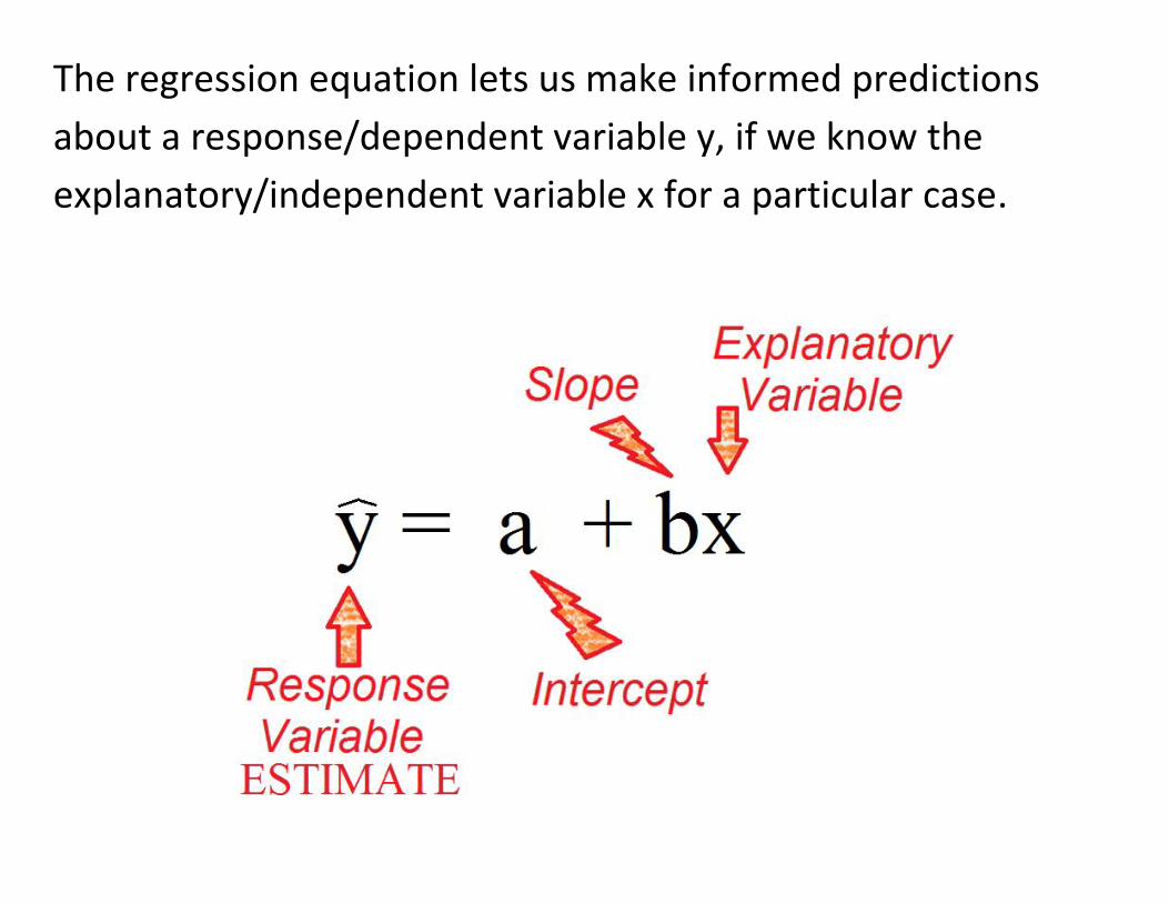
The regression equation lets us make informed predictions

about a response/dependent variable y, if we know the

explanatory/independent variable x for a particular case.

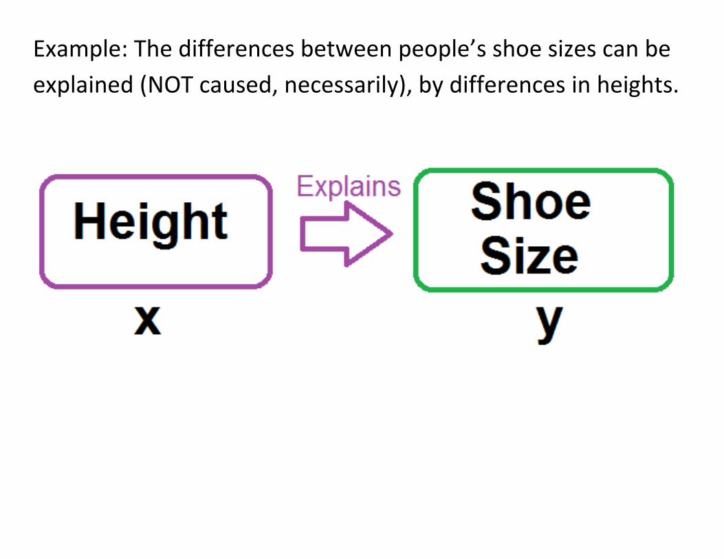
Example: The differences between people’s shoe sizes can be

explained (NOT caused, necessarily), by differences in heights.

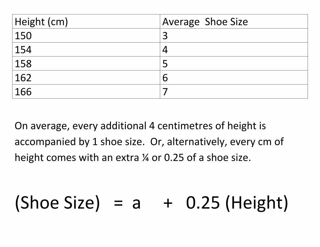
Height (cm) Average Shoe Size 150 3 154 4 158 5 162 6 166 7

On average, every additional 4 centimetres of height is

accompanied by 1 shoe size. Or, alternatively, every cm of

height comes with an extra ¼ or 0.25 of a shoe size.

(Shoe Size) = a + 0.25 (Height)

Height (cm) Average Shoe Size 0 -34.5 4 -33.5 … … 142 1 146 2 150 3

If we follow this pattern back to a height of 0 centimeters, we

get size -34.5 shoes.

(Shoe Size) = -34.5 + 0.25 (Height)

(Shoe Size) = -34.5 + 0.25 (Height)

Nobody is 0cm tall, so the value at Height x = 0 is has no real

world meaning, but it does allow us to plug in a height and get

a shoe size out.

(Shoe Size) = -34.5 + 0.25 (171)

= 8.25

Are we completely sure this person has size 8.25 shoes? (Even

if shoes were made in that size)

Name Height Shoe Size Capt. Janeaway 170 8 Manfried Maxx 170 7 Inspector Vimes 170 9

Not every person of the same height has the same size shoes.

All we’re dealing with the average shoes of someone of that

height.

There’s some variation in shoe sizes between people of the

same height. That’s the variance left unexplained, the

errors/residuals.

Name Height Shoe Size Capt. Janeaway 170 8 Manfried Maxx 170 7 Inspector Vimes 170 9

To account for this unexplained variance, we could

a) Write it in as an error term .

(Shoe Size) = -34.5 + 0.25 (Height) + Error

This way, the formula for shoe size is exact, but depends on

the error, which the linear model can’t explain.

Or we could…

b) Use the formula to estimate shoe sizes rather than give

then exactly.

(Estimated Shoe Size) = -34.5 + 0.25 (Height)

The error terms are, on average zero, so we’re not

systematically over or under estimating the response (y, shoe

size). In other words, our estimate is unbiased .

Estimations of something are given a symbol above them,

instead of writing “estimated” every time. Usually, it’s a hat.

So, bringing everything back into symbols:

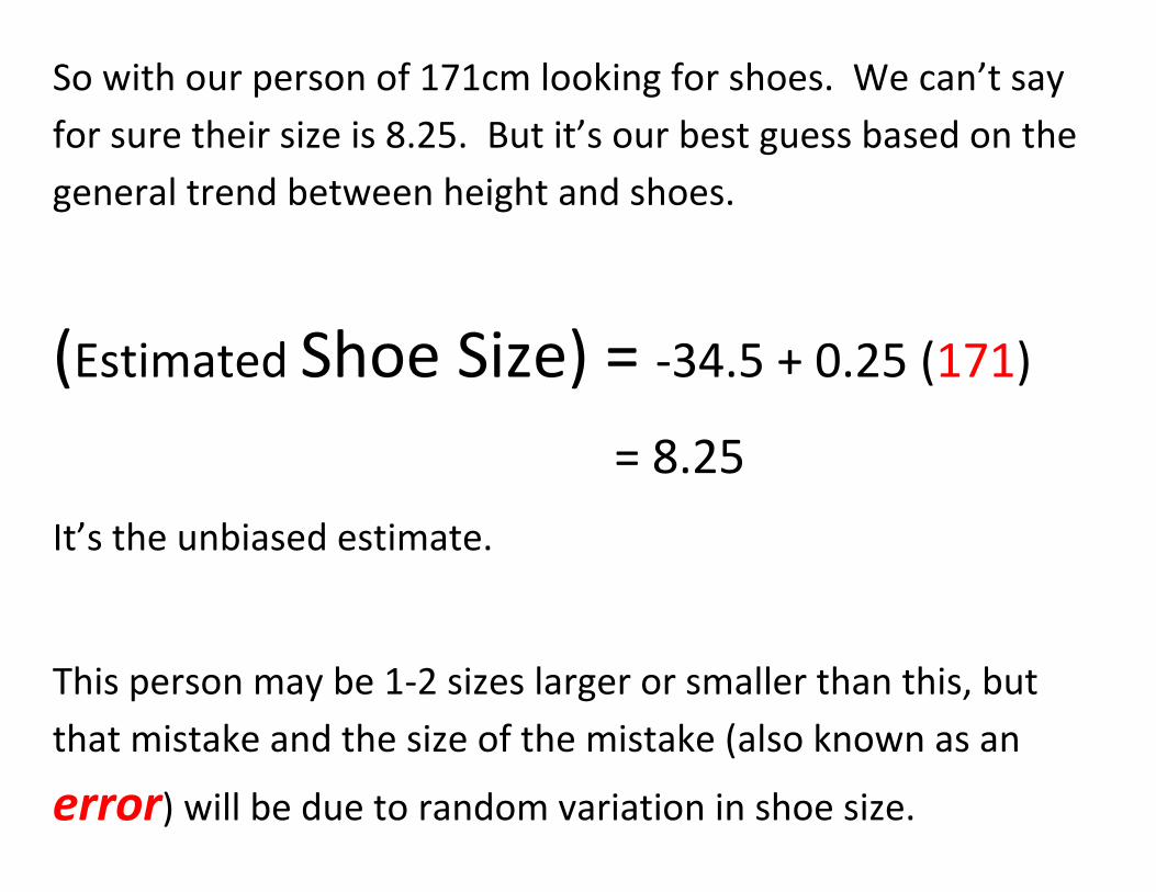
So with our person of 171cm looking for shoes. We can’t say

for sure their size is 8.25. But it’s our best guess based on the

general trend between height and shoes.

(Estimated Shoe Size) = -34.5 + 0.25 (171)

= 8.25

It’s the unbiased estimate.

This person may be 1-2 sizes larger or smaller than this, but

that mistake and the size of the mistake (also known as an

error) will be due to random variation in shoe size.

What would a biased estimate look like? Anything that has

systematic (not random) errors.

- Someone who always guessed shoe sizes a couple of sizes

too big would be making a systematic error. He/She would

be biasing towards larger shoes.

- Someone who estimated based on 2cm = 1 size, rather

than 4cm/size would also be making biased estimates,

although they might give extra small shoes to short people

and extra big shoes to tall people.

But I hope this does not bias you against using regression, it’s

part of a complete statistics diet.

The quality of a prediction depends on how much variance is

left unexplained.

If there were none left unexplained, then the x values would

be in a perfect linear relationship with y. Plugging an x value

into this equation would give you the y value exactly.

The estimate would be dead-on every time, a perfect

prediction.

This happens when

r = -1 or 1, and therefore r2 = 1.

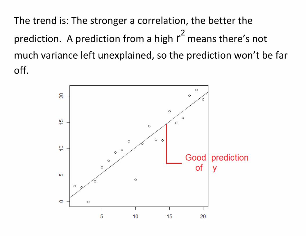
The trend is: The stronger a correlation, the better the

prediction. A prediction from a high r2 means there’s not

much variance left unexplained, so the prediction won’t be far

off.

A low r2 means lots of unexplained variation in the response y.

That means any prediction of y is going to be vague to account

for the variation.

Sometimes we have more than one variable we could use to

predict something.

We could pick the one with stronger correlation (highest r2 ) to get a picture of how one thing changes as another thing

changes.

Often a better way to describe the patterns in a response

variable is to consider two or more explanatory variables at the

same time.

Describing the patterns in a response is also called

modelling the response, or building a model of the

response.

r2 = .467 between Hours and Grade

r2 = .760 between Skill and Grade

The r2 of a multiple regression is ALWAYS at least as high as

the r2 of any of single regressions from using only one of the

variables.

All the increase in r2 means is that both variables together

explain more of the variation in the response than either one

of them could on their own.

There’s no nice formula to get the multiple regression r2, so

we depend on software like SPSS to do it for us.

The formula for this multiple regression is:

(Exam Grade) = a + b1(Study hours) + b2(Skill)

a = Grade for someone with 0 study hours AND 0 skill.

b1 = The change in Grade for each additional 1 hour studied

holding skill constant.

b2 = The change in Grade for each additional 1 point of skill

holding study time constant.

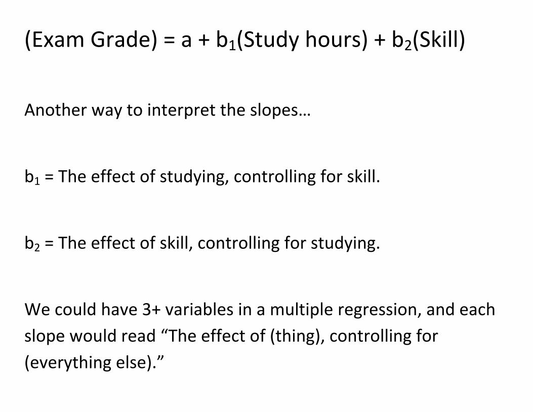
(Exam Grade) = a + b1(Study hours) + b2(Skill)

Another way to interpret the slopes…

b1 = The effect of studying, controlling for skill.

b2 = The effect of skill, controlling for studying.

We could have 3+ variables in a multiple regression, and each

slope would read “The effect of (thing), controlling for

(everything else).”

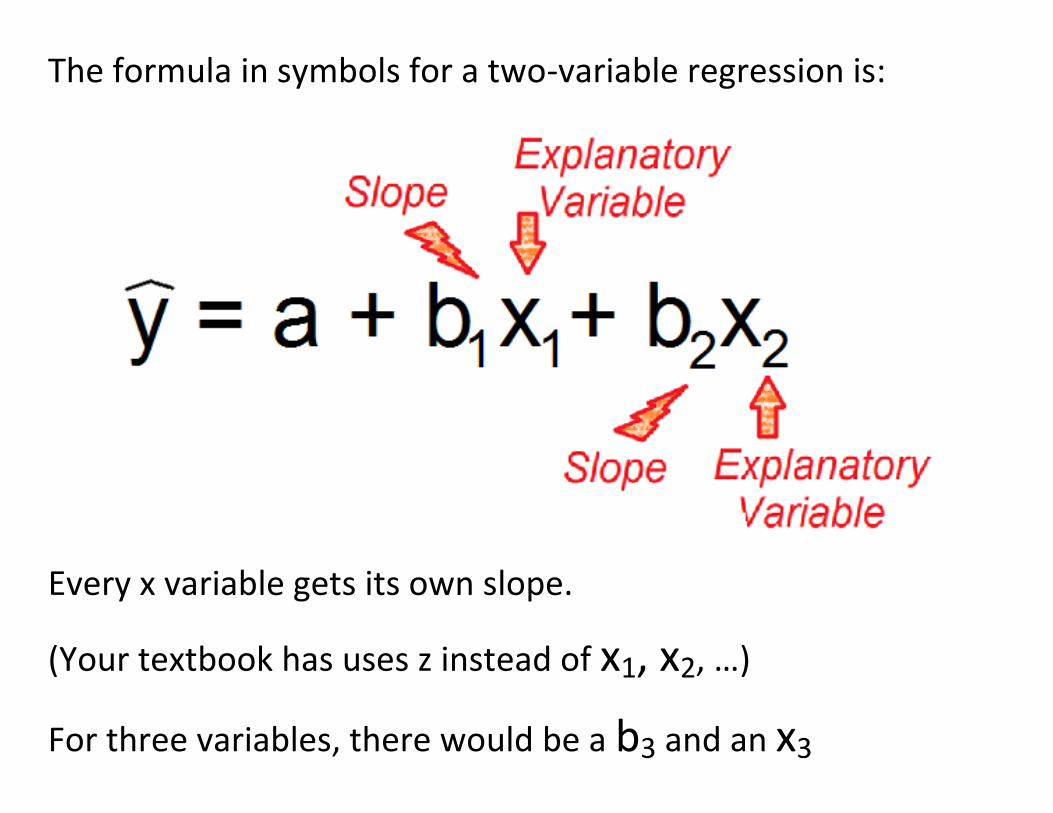
The formula in symbols for a two-variable regression is:

Every x variable gets its own slope.

(Your textbook has uses z instead of x1, x2, …)

For three variables, there would be a b3 and an x3

Cenote: Opening to underwater caverns found in the rainforest

Multiple regression in SPSS starts the same as single

regression.

Analyze Regression Linear

In the Linear Regression pop up, move your y variable into

dependent and ALL the x variables you wish to include into

independent.

In this case, we’re using the NHL dataset, and we’re modelling

the number of Wins a team gets as function of how many goals

they score (GF) and how many are scored on them (GA).

Then click OK.

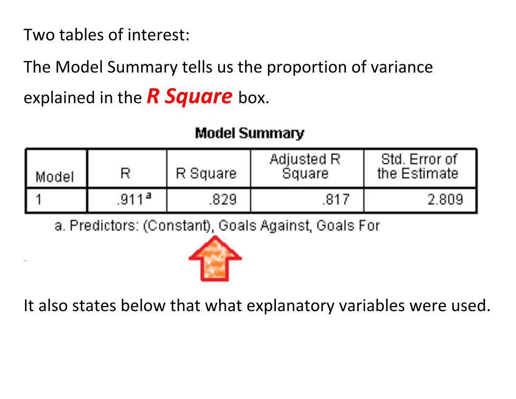
Two tables of interest:

The Model Summary tells us the proportion of variance

explained in the R Square box.

It also states below that what explanatory variables were used.

The coefficients table tells you what the slopes are (first arrow)

And the p-value against each of those slopes being zero.

(second arrow)

A team that scored no goals and let no goals in gets 37.95 wins

on average. (Out of a regular season of 82 games, so a little

fewer than half)

Since predicting for 0 goals against, 0 goals for is extrapolating,

this is only an mathematical starting point.

For every 1 goal scored, a team won 0.177 more games.

Teams that score more often win more, no surprize.

Also, this slope is very significant (p-value near .000), so we’re

very sure it isn’t zero.

For every 1 goal that a team let in, they won 0.163 fewer

games.

In other words, teams that were better defensively (let in

fewer goals) won more.

This is also highly significant with p-value near .000

For the Goals For slope, that’s controlling for Goals Against.

That means we’re looking at the increase in wins of a team

that scores more goals but does NOT let more in.

That way we’re looking at the effect of offense ability alone.

Let’s use this for prediction.

(Estimated Wins) = 37.95 + 0.177(GF) – 0.163(GA)

How many wins would a team that scores 220 goals and lets

210 goals in get, on average? (Moderate offence/defence)

Wins =

37.95 + 0.177 ( 220 ) - 0.163 ( 210 )

= 42.66 So they would win a little more than half their games.

Another prediction:

(Estimated Wins) = 37.95 + 0.177(GF) – 0.163(GA)

How many wins would a team that scores 160 goals, but only

lets in 130 get, on average. (Very low scoring games)

Wins =

37.95 + 0.177 ( 160 ) - 0.163 ( 130 )

= 45.08

The Prince George Potato Sacks are a theoretical NHL team,

which includes 19 sumo wrestlers. Their job is to pile in front

of their net and form a wall. The wall isn’t perfect.

They score 0 goals but only let in 21. How many wins does our

model say they should get.

Wins =

37.95 + 0 - 0.163 ( 21 ) = 34.53 Is this reasonable?

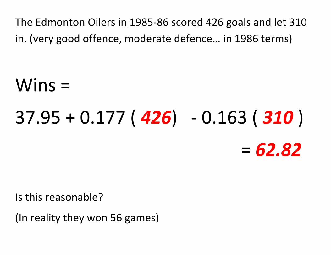
The Edmonton Oilers in 1985-86 scored 426 goals and let 310

in. (very good offence, moderate defence… in 1986 terms)

Wins =

37.95 + 0.177 ( 426) - 0.163 ( 310 )

= 62.82

Is this reasonable?

(In reality they won 56 games)

This model only uses data from the 2011-12 regular season.

We couldn’t use it for other seasons where there are different

teams and different rules.

We also couldn’t use it to predict the wins of teams that would

get far from the usual amount of goals for or against.

Both of these cases are extrapolation, making predictions for

situations that weren’t within the data we used to build the

predictions in unreasonable.

Playoff wins = a + (negative number) ( water bottle skills) ?

Next time: Dummy variables.