regression: introduction call this e(y | x)

1

Regression: IntroductionPsychology 6140

2

Prototype example: Ozone in LA

How does atmospheric ozone in LA depend on temperature?• Consider many small slices (x)• For each x, find average y• Call this E(y | x)

In general, we want to be able to describe / predict how a response (y) is related to one (or more) explanatory variables (x)

But --- possibly different goals:• simple description (given data)• prediction (future data)• causal explanation – mechanism?

3

Prototype example: Ozone in LA

If the averages, E(y | x) can be assumed to be linearly related to x, we have a simple linearregression model,

0 1( | )E y x x

Such a description is alwaysapproximate:

• the true relation of y to x may not be exactly linear (as here)

• y may also depend on other x’s

Nevertheless, this is a model we can extend 4

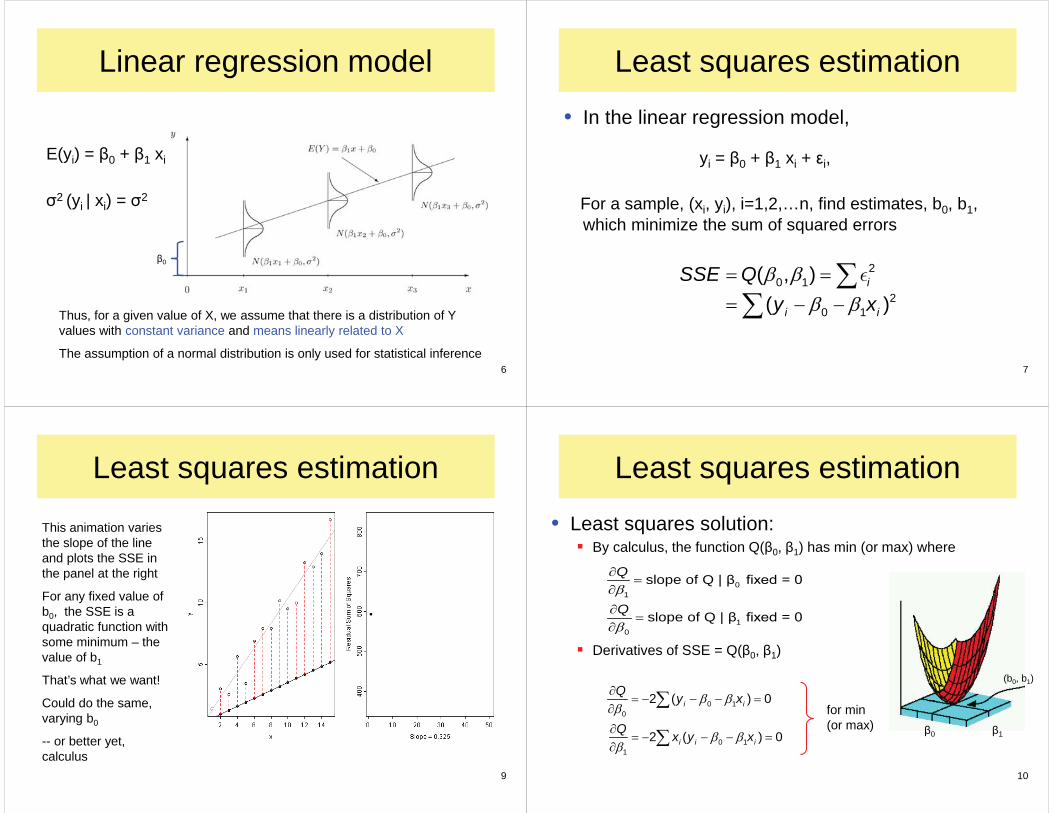
Linear regression model• Model: yi = 0 + 1 xi + i, where

• Assumptions:Unbiased: E( i ) = E(y|x) only x mattersIndependence: cov( i, j) = ( i, j independent samplingHomogeneity of variance: var( i) = 2 ( i) = 2

• Implies:For each xi there is a (hypothetical) distribution of yi values, with

E(yi) = 0 + 1 xi (linear regression)2 (yi | xi) = 2 (constant error variance)

0, 1 : fixed, unknown

xi : fixed, knownfixed random

In application, assumption of fixed x is unrealistic and not necessary. OK as long as residuals meet the assumptions.

6

Linear regression model

E(yi) = 0 + 1 xi

2 (yi | xi) = 2

Thus, for a given value of X, we assume that there is a distribution of Y values with constant variance and means linearly related to X

The assumption of a normal distribution is only used for statistical inference

0

7

Least squares estimation

• In the linear regression model,

For a sample, (xi, yi), i=1,2,…n, find estimates, b0, b1,which minimize the sum of squared errors

yi = 0 + 1 xi + i,

20 1

20 1

( , )( )

i

i i

SSE Qy x

9


This animation varies the slope of the line and plots the SSE in the panel at the right

For any fixed value of b0, the SSE is a quadratic function with some minimum – the value of b1

That’s what we want!

Could do the same, varying b0

-- or better yet, calculus

10


• Least squares solution:By calculus, the function Q( 0, 1) has min (or max) where

Derivatives of SSE = Q( 0, 1)

01

10

slope of Q |

slope of Q |

Q

Q

0 10

0 11

2 ( ) 0

2 ( ) 0

i i

i i i

Q y x

Q x y x

for min (or max)

0 1

(b0, b1)

11


• Simplifying

• Solve for b0, b1:

0 12

0 1

i i

i i i i

y nb b xx y b x b x

0 1 1

1 2 2

( ) /( )( )( )

i i

i i i i

i i

y x y b xx

b b nn x yb y

x xn

02

1

i i

i i i i

y xx

by x

nx b

0 -1

1

T Tbb

b = (X X) X y

Two equations in 2 unknowns

Solution exists if (XT X) is non singular

12

Regression: Matrix notation• Model:

• Assumptions:

• Least squares:

• Normal eqns:

• LS solution:

1 1 10

1

1

1n n n

y x

y x

2~ ( , )iid

I

2 12 11 nnny X

min ( () )T TQ XX

02

1

i i

i i i i

ny

x yx x x ( )T TX X b X yor,

-1T Tb = (X X) X y

“iid”: independent and identically distributed

13

Regression: Matrix notation

• Fitted values:

• Residuals:

• Residual SS:

• Std errors:

1)ˆ ( T TXy Xb XX yX Hy

( )e y Xb I H y

( )

T T T

T

SSE y y b X yy I H y

02 1

1

2

( )

1/( ) 1

T

n xMSEx x x

bs MSE

bX X

14

Example: Improvement in Therapy

NAME SEX PERSTEST THERAPY INTEXT SX

John M 26 32 3 0Susan F 24 40 4 1Mary F 22 44 8 1Paul M 33 44 4 0Jenny F 27 48 6 1Rick M 36 52 4 0Cathy F 30 56 10 1Robert M 38 56 4 0Lisa F 30 60 12 1Tina F 34 68 15 1

25 30 35

3540

4550

5560

65

perstest: Personality Test

ther

apy:

Impr

ovem

ent i

n Th

erap

y

x y

proc reg data=therapy; model therapy = perstest; run;

Parameter Estimates Parameter StandardVariable DF Estimate Error t Value Pr > |t|

Intercept 1 14.000 17.204 0.81 0.4393PERSTEST 1 1.200 0.566 2.12 0.0667

therapy 14 1.2 perstest

lm(therapy ~ perstest, data = therapy)

15

Statistical Inference: Regression

16


Classical statistical inference: Use the sample estimate (b1) to draw a conclusion about population value ( 1)

• Two types: (a) hypothesis tests; (b) confidence intervals

Hypothesis test: 0 1

1 1

: 0: 0

HH

Confidence interval: Find c such that

1 1 1 1 1Pr Pr 1c cb b b c

“Is there evidence that the true slope is different from 0?”

“What range around b1 includes the true value 1 with probability 1- ?”

These are equivalent, in the sense that if the CI includes 0, the hypothesis test will not reject H0.

17

Statistical Inference: RegressionHow to go from our single sample estimate (b1) to the population value ( 1)?

The key idea was that of the sampling distribution of a statistic like b1.

18


Here we simulated 500 samples from a linear regression in which

yi = 14 + 1.2 x + i

and i ~ N(0, 80)

mean b1 1 = 1.2

std dev b1 ( 1) = 0.566

The theoretical 95 % CI for 1 is shown by the dotted red lines

19


20

Regression with SAS: therapy data

2

The REG ProcedureDependent Variable: THERAPY

Analysis of Variance

Sum of MeanSource DF Squares Square F Value Pr > F

Model 1 360.00000 360.00000 4.50 0.0667Error 8 640.00000 80.00000Corrected Total 9 1000.00000

Root MSE 8.94427 R-Square 0.3600Dependent Mean 50.00000 Adj R-Sq 0.2800Coeff Var 17.88854

Parameter Estimates

Parameter StandardVariable DF Estimate Error t Value Pr > |t|

Intercept 1 14.00000 17.20465 0.81 0.4393PERSTEST 1 1.20000 0.56569 2.12 0.0667

proc reg data=therapy;model therapy = perstest / p;output out=results p=fitted r=residual;id name;run;

options

output stats

overall model: H0: R2 = 0

22

Confidence bands• To understand uncertainty in

predicted y, it is useful to calculate and display confidence bands

• For a given value, x = xh

• In SAS, the option is CLM

whereˆ (1 )T Th h h hxy xx b

2 1( ( )ˆ ) T T Th h hy MSEs x X X x

proc reg data=therapy;model therapy = perstest / CLM; NB: CI gets larger as we

move away from mean of X23

Confidence bands

The simulation results show why uncertainty increases with distance2 from the mean of x

22

2

( )1ˆ ))

((

hh

i

x xy MSEn

sx x

Note that these are limits for the mean predicted value (CLM), not for any individual (CLI)

24

Vector geometry of least squares fit

Model:

0 1

ˆ ey1 x

ye

Minimizing ei2 = ||e||2

projection of y onto plane of x and 1

In matrix form:

y

1

( )( 1) ( 1)whereˆ )( T T

n nn nX X Xy H H Xy Diagonal elements, hii of

the “hat” matrix are measures of “leverage” 25

Vector geometry of least squares fit

• The vector geometry of regression can be shown in 2D by expressing variables in mean deviation form

• Original model: yi = b0 + b1 x + ei

• Deviation form:

• Then,

1( () )i i iy xy b x e

1by ey e x

yi* xi*

Example: regvec3d

26

The matlib function regvec3d() extends this idea to two predictors, calculating a 3D vector representation of the model y ~ x1 + x2, in deviation form.

The result can be viewed in 2D or 3D accurately reflecting the partial relations of y to x1 and x2.

therapy.vec <- regvec3d(therapy ~ perstest + IE, data=therapy)plot(therapy.vec)plot(therapy.vec, dimension=2)

27

Vector geometry: ANOVA sums of squares

The ANOVA sums of squares are just the squared lengths of these vectors

2 2 2|| || || || ||ˆ ||SSTO SSR SSEy ey

ANOVA:

df: # of dimensions (n-1) = 1 + (n-2)

R squared:

R2 = SSR / SSTOcorrelation: r = cos ( )

28

Vector geometry: Derivation of LS fit

• In the model y = (1, x) b + e = X b + e, the residual vector, e, is orthogonal to plane of (1, x)

• This provides another derivation of the LS solution

(1, x)T e = XT e = 0 XT (y-Xb) = 0 XT y – XT X b = 0 XT X b = XT y b = (XT X)-1 XT y

29

Multiple regressionLinear model with two independent variables

30

Multiple regressionLinear in x1 and x2 means:• we can interpret the slopes b1 and b2 w/o regard for the other variable• at the same time, we are controlling for the other variable

31

Multiple regression: therapy data



Model 2 922.42744 461.21372 41.62 0.0001Error 7 77.57256 11.08179Corrected Total 9 1000.00000


Parameter Estimates


Intercept 1 2.82850 6.59255 0.43 0.6808PERSTEST 1 1.12296 0.21082 5.33 0.0011INTEXT 1 1.92612 0.27037 7.12 0.0002

proc reg data=therapy;model therapy = perstest intext;run;

Partial tests(more later)

Overall model test

32


Fitted response surface: 2.83 1.12 1.92 therapy perstest intext

33


What about sex? (or other x’s)

• Residual plots should show no systematic structure

• Here, females tend to have + residuals, suggesting an additional effect of sex on therapy outcome

34


proc reg data=therapy;model therapy = perstest intext sx;run;



Model 3 982.05152 327.35051 109.43 <.0001Error 6 17.94848 2.99141Corrected Total 9 1000.00000


Parameter Estimates


Intercept 1 -14.79157 5.22575 -2.83 0.0299PERSTEST 1 1.71897 0.17268 9.95 <.0001INTEXT 1 0.96956 0.25620 3.78 0.0091SX 1 10.72600 2.40251 4.46 0.0043

Dummy (0/1) for sex

35


Model 2: ignoring Sex Model 3: including Sex

Benefits: Residuals no longer associated with sex Residual SSE now considerably smaller: smaller std errors

36

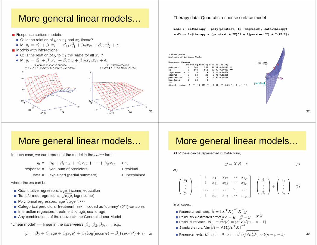
More general linear models…

37

Therapy data: Quadratic response surface model

mod3 <- lm(therapy ~ poly(perstest, IE, degree=2), data=therapy)

mod3 <- lm(therapy ~ (perstest + IE)^2 + I(perstest^2) + I(IE^2))

> anova(mod3)Analysis of Variance Table

Response: therapyDf Sum Sq Mean Sq F value Pr(>F)

perstest 1 360 360 60.12 0.00149 ** IE 1 562 562 93.93 0.00063 ***I(perstest^2) 1 14 14 2.27 0.20638I(IE^2) 1 23 23 3.76 0.12455perstest:IE 1 18 18 2.93 0.16228Residuals 4 24 6---Signif. codes: 0 ‘***’ 0.001 ‘**’ 0.01 ‘*’ 0.05 ‘.’ 0.1 ‘ ’ 1

38


39


40

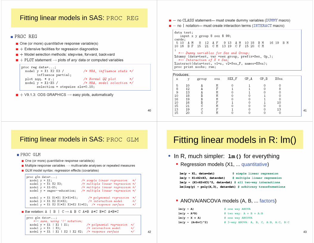
Fitting linear models in SAS: PROC REG

41

42

Fitting linear models in SAS: PROC GLM

43

Fitting linear models in R: lm()• In R, much simpler: lm() for everything

Regression models (X1, ... quantitative)

ANOVA/ANCOVA models (A, B, ... factors)

lm(y ~ X1, data=dat) # simple linear regression

lm(y ~ X1+X2+X3, data=dat) # multiple linear regression

lm(y ~ (X1+X2+X3)^2, data=dat) # all two-way interactions

lm(log(y) ~ poly(X,3), data=dat) # arbitrary transformations

lm(y ~ A) # one way ANOVA

lm(y ~ A*B) # two way: A + B + A:B

lm(y ~ X + A) # one way ANCOVA

lm(y ~ (A+B+C)^2) # 3-way ANOVA: A, B, C, A:B, A:C, B:C

lm(y ~ X1, data=dat) # simple linear regression

lm(y ~ X1+X2+X3, data=dat) # multiple linear regression

lm(y ~ (X1+X2+X3)^2, data=dat) # all two-way interactions

lm(log(y) ~ poly(X,3), data=dat) # arbitrary transformations

44

Fitting linear models in R: lm()• Multivariate models: lm() for everything

Multivariate regression

MANOVA/MANCOVA models

lm(cbind(y1, y2) ~ X1 + X2 + X3) # std MMreg: all linear

lm(cbind(y1, y2) ~ poly(X1,2) + poly(X2,2)) # response surface

lm(cbind(y1, y2, y3) ~ A * B) # 2-way MANOVA: A + B + A:B

lm(cbind(y1, y2, y3) ~ X + A) # MANCOVA (equal slopes)

lm(cbind(y1, y2) ~ X + A + X:A) # heterogeneous slopes

45

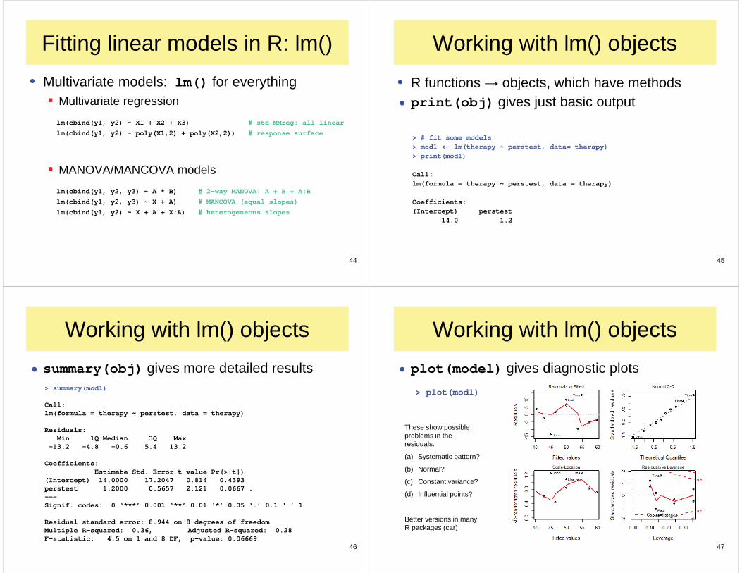
Working with lm() objects

• R functions objects, which have methods• print(obj) gives just basic output

> # fit some models> mod1 <- lm(therapy ~ perstest, data= therapy)> print(mod1)

Call:lm(formula = therapy ~ perstest, data = therapy)

Coefficients:(Intercept) perstest

14.0 1.2

46

Working with lm() objects• summary(obj) gives more detailed results

> summary(mod1)

Call:lm(formula = therapy ~ perstest, data = therapy)

Residuals:Min 1Q Median 3Q Max

-13.2 -4.8 -0.6 5.4 13.2

Coefficients: Estimate Std. Error t value Pr(>|t|)(Intercept) 14.0000 17.2047 0.814 0.4393 perstest 1.2000 0.5657 2.121 0.0667 .---Signif. codes: 0 ‘***’ 0.001 ‘**’ 0.01 ‘*’ 0.05 ‘.’ 0.1 ‘ ’ 1

Residual standard error: 8.944 on 8 degrees of freedomMultiple R-squared: 0.36, Adjusted R-squared: 0.28 F-statistic: 4.5 on 1 and 8 DF, p-value: 0.06669

47

Working with lm() objects• plot(model) gives diagnostic plots

> plot(mod1)

These show possible problems in the residuals:

(a) Systematic pattern?

(b) Normal?

(c) Constant variance?

(d) Influential points?

Better versions in many R packages (car)

48

Working with lm() objects

• anova() tests differences among nested models> mod2 <- lm(therapy ~ perstest + intext, data=therapy)> mod3 <- lm(therapy ~ perstest + intext + sex, data=therapy)> anova(mod1, mod2, mod3)Analysis of Variance Table

Model 1: therapy ~ perstestModel 2: therapy ~ perstest + intextModel 3: therapy ~ perstest + intext + sexRes.Df RSS Df Sum of Sq F Pr(>F)

1 8 640.00 2 7 77.57 1 562.43 188.014 9.352e-06 ***3 6 17.95 1 59.62 19.932 0.004262 ** ---Signif. codes: 0 ‘***’ 0.001 ‘**’ 0.01 ‘*’ 0.05 ‘.’ 0.1 ‘ ’ 1

Note: these are so-called “Type I” (sequential) tests, testing the additional contribution of each new predictor. Other (“Type II”) tests are more generally useful. 49

Summary, to here

• Simple linear regression:Fit a model predicting E(y | x) = 0 + 1 xUse least squares to find estimates, b0, b1

Matrix solution:

• Multiple regression:Include any number of linear predictorsE(y | x) = 0 + 1 x1 + 2 x2 + …Partial coefficients: Effect of xi controlling for othersCan include terms like x2,x3, x1*x2, factor variables, etc.For all, -1T Tb = (X X) X y

-1T Tb = (X X) X y

2 1 (( ) )Ts MSE Xb X

50

What we still have to learn• Model assessment

How to judge the contributions of different Xs?• Type I (sequential) and Type II (partial) tests• Principle of marginality (main effects & interactions)

Ordered (“hierarchical”) tests• Model diagnosis

How to see and test for violations of assumptionsRegression diagnostics: influential observations???Detecting and dealing with collinearity

• Model building/selection strategiesHow to select an adequate/optimal subset of predictorsDangers of “stepwise” selectionCross-validation, shrinkage, LASSO methods

regression: introduction call this e(y | x)

Documents