Regression Part 3 of 3 Parts•Multiple Regression Overview• Examples• Hypothesis Tests• MR ANOVA Table• Interpretation• Indicator Variables• Assumptions• Homework• Up Next

-Model Building-MR Interaction

Multiple Regression Overview

• Study of how several variables are related or associated with one dependent variable. For example applications review chapter problem scenarios.

• Several independent variables may be interval/continuous or categorical/dummy/indicator.

• Interval and categorical variables may both be included simultaneously in the MR model.

• Predict or estimate the value of one variable based on the others.

€

H0 : β1 = β 2 = ...β k = 0

H1 : At least one β i is not equal to 0 (the model has some validity)

At least one of the independent variables is related to the dependent variable

Example Application

From Keller, Statistics for Management & Economics, 8E.

The Multiple Regression Model

Four (4) continuous/interval independent variables.

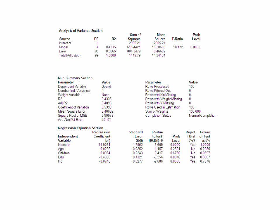
Interpreting the Regression Coefficients

Testing the Regression Coefficients

Source df SS MS F

Regression k SSR MSR=SSR/1 F*=MSR/MSE

Error n-k-1 SSE MSE=SSE/(n-2) Fcrit=F ,k,n-k-1

Total n-1 SST

ANOVA Table for Basic Multiple Regression

Indicator/Dummy/Categorical Independent Variables in Multiple Regression

•Categorical variables represent data that can be organized into groups.

•Remember categorical variables can also be either nominal or ordinal.

•With categorical data we may count up (in whole numbers) the number of observations that fall in a group or category.

•Examples: ethnicity, gender, class grade, classification, rank, yes/no data groups, bond rating, number of automobiles a family owns, income group (low/med/high), political affiliation, age bracket . . .

•For each categorical family, we use the number of categories minus 1 variables in the MR model.

From Keller, Statistics for Management & Economics, 8E.

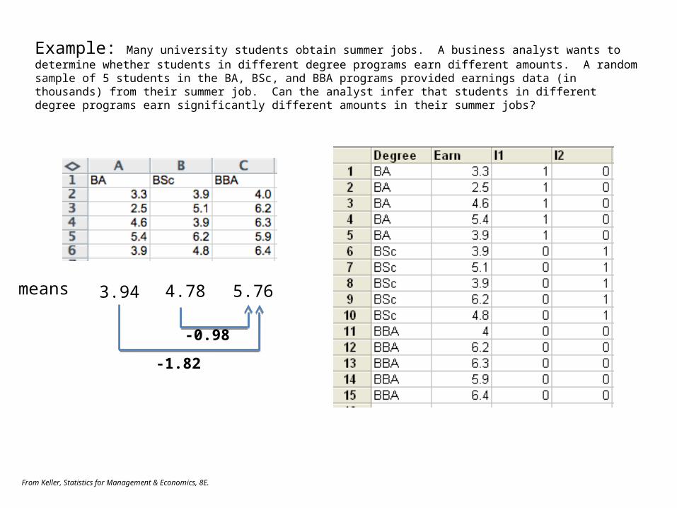
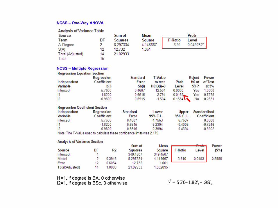
Example: Many university students obtain summer jobs. A business analyst wants to determine whether students in different degree programs earn different amounts. A random sample of 5 students in the BA, BSc, and BBA programs provided earnings data (in thousands) from their summer job. Can the analyst infer that students in different degree programs earn significantly different amounts in their summer jobs?

means 3.94 4.78 5.76

-1.82

-0.98

€

ˆ Y = 5.76−1.82I1 − .98I2

Interpreting

14.49Page 557

32.5

60.4

53.1

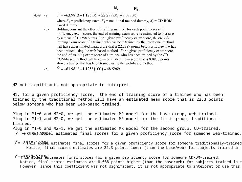
M1 M2

M2 not significant, not appropriate to interpret.

M1, for a given proficiency score, the end of training score of a trainee who has been trained by the traditional method will have an estimated mean score that is 22.3 points below someone who has been web-based trained.

Plug in M1=0 and M2=0, we get the estimated MR model for the base group, web-trained.Plug in M1=1 and M2=0, we get the estimated MR model for the first group, traditional-trained.Plug in M1=0 and M2=1, we get the estimated MR model for the second group, CD-trained.

€

ˆ Y = −63.98 +1.126X1This model estimates final scores for a given proficiency score for someone web-trained, the base.

€

ˆ Y = −86.27 +1.126X1 This model estimates final scores for a given proficiency score for someone traditionally-trained.Notice, final scores estimates are 22.3 points lower (than the base/web) for subjects trained in this way.

€

ˆ Y = −55.89 +1.126X1 This model estimates final scores for a given proficiency score for someone CDROM-trained.Notice, final scores estimates are 8.088 points higher (than the base/web) for subjects trained in this way.However, since this coefficient was not significant, it is not appropriate to interpret or use this (third) model.

M1 M2

To obtain a 95% CI for a point estimate:

There are certain assumptions that must be met or need to be near met for our method of least squares and results to be valid. e~iid(0,2)

LINE L – Linearity I – Independence of errors N – Normality E – Equal Variance

Assumptions

Linearity

Only for the interval/continuous variable(s)

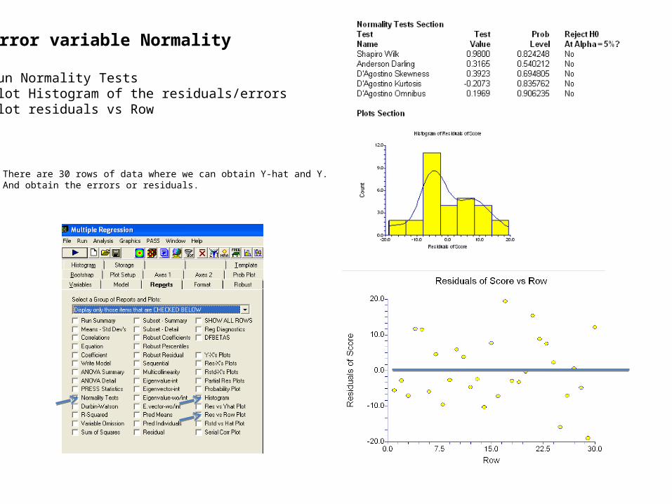
Error variable Normality

Run Normality TestsPlot Histogram of the residuals/errorsPlot residuals vs Row

There are 30 rows of data where we can obtain Y-hat and Y.And obtain the errors or residuals.

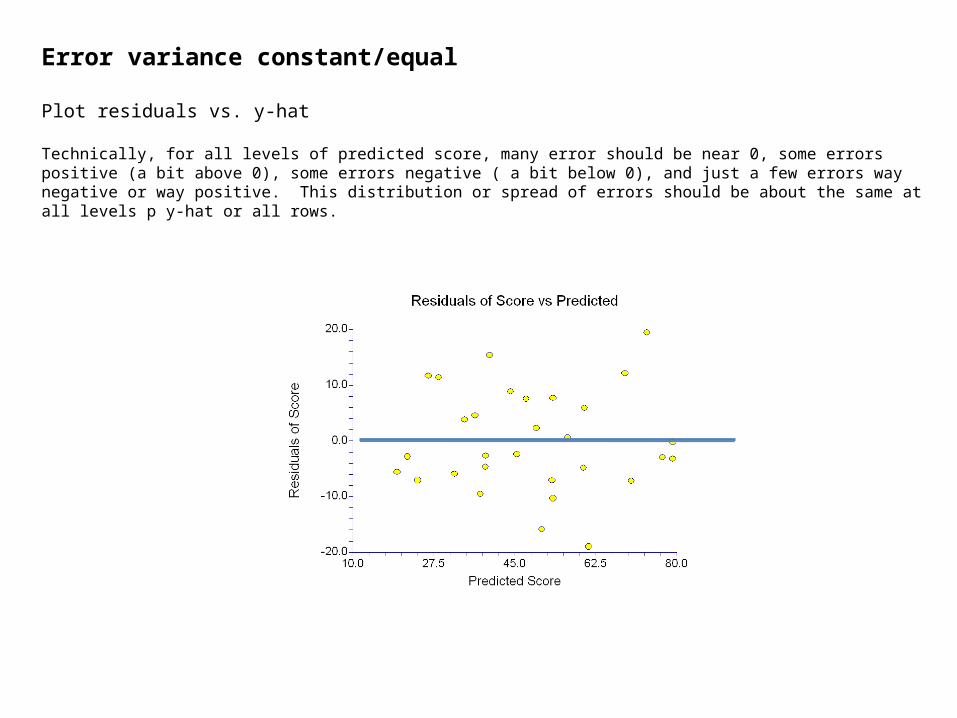
Error variance constant/equal

Plot residuals vs. y-hat

Technically, for all levels of predicted score, many error should be near 0, some errors positive (a bit above 0), some errors negative ( a bit below 0), and just a few errors way negative or way positive. This distribution or spread of errors should be about the same at all levels p y-hat or all rows.

Errors Independent

Durbin-Watson test, page 494+Plot residuals vs each i.v.

The errors should be independent and neither positively correlated (for each successive row increasing) nor negatively correlated (for each successive row decreasing). Also plot errors vs each independent variable.

€

H0 : the errors are independent

H1 : the errors are not indepent (they are dependent or related)

okay not

okay

The accuracy of the model should be the same at any profic level. In this plot,higher profic scores produce greater positive errors, the model gets increasingly worse.

Multicollinearity

Model Building page 584+

Homework (#5) Multiple Regression

14.45a.b.c. Use the MR model to predict the cost for a restaurant with a summated rating of 60 that is located in the city. Use NCSS to obtain the CI.d. Perform a basic MR assumption coherence/violation analysis.e. f. Interpret the regression equation and regression coefficients.