regular paper - unina.itwpage.unina.it/donato.amitrano/publications/journals/2015_ijrs... · bbfs....

July 5, 2015 International Journal of Remote Sensing Errico2014˙rev7

International Journal of Remote SensingVol. 00, No. 00, 00 Month 201X, 1–21

regular paper

Detection of environmental hazards through the feature-based

fusion of optical and SAR data: a case study in southern Italy

Angela Erricoa, Cesario Vincenzo Angelinoa, Luca Cicalaa, Giuseppe Persechinoa,

Claudia Ferrarab, Massimiliano Legab, Andrea Vallarioc, Claudio Parentec,

Giuseppe Masid,e, Raffaele Gaetanod,e, Giuseppe Scarpad,e, Donato Amitranod,

Giuseppe Ruellod, Luisa Verdolivad,e, and Giovanni Poggid,e ∗

aCIRA, the Italian Aerospace Research Center, Capua, Italy ;bDepartment of Engineering, University Parthenope of Naples, Italy ;

cDepartment of Sciences and Technologies, University Parthenope of Naples, Italy ;dDIETI, University Federico II of Naples, Italy ;

eCNIT, National Inter-University Consortium for Telecommunications, Italy ;

(Received 00 Month 201X; final version received 00 Month 201X)

The use of remote-sensing images is becoming common practice in the fight againstenvironmental crimes. However, the challenge of exploiting the complementary infor-mation provided by radar and optical data, and by more conventional sources encodedin geographic information systems, is still open. In this work, we propose a new work-flow for the detection of potentially hazardous cattle-breeding facilities, exploitingboth synthetic aperture radar and optical multitemporal data together with geospa-tial analyses in the geographic information system environment. The data fusion isperformed at a feature-based level. Experiments on data available for the area ofCaserta, in southern Italy, show that the proposed technique provides very high de-tection capability, up to 95%, with a very low false alarm rate. A fast and easy-to-usesystem has been realized based on this approach, which is a useful tool in the hand ofagencies engaged in the protection of territory.

Keywords: Multisensor data fusion, synthetic aperture radar, GIS, image analysis,environmental hazard detection, digital image forensics.

1. Introduction

Enforcement of environmental regulation is a persistent challenge, and timely de-tection of violations is key to holding violators accountable. Typically, the inves-tigation is triggered by the evidence of the damage, rather than of the illegalpolluting act. Often, the effects appear a long time after the polluting act has beencommitted, and in a different place. The correlation between the source and thedamage depends upon the morphology of the scenario and the physical phenom-ena that allow the transport of the pollutants (Lega et al. 2012a). In these cases,the effectiveness of investigations can be greatly enhanced by using remote-sensingdata and information technology tools. Continuous and targeted monitoring allowsfor efficient police action (Lega and Napoli 2010; Pringle et al. 2012). Successfulidentification and prosecution of culprits requires an integrated system based on

∗Corresponding author. email: [email protected]

1


data from several sources, including space, air, waterways, and land monitoring(Lega et al. 2012b).

Environmental monitoring and analysis - and in particular the detection andmonitoring of environmental crimes - can produce complex data that are diffi-cult to represent. For these purposes, the use of geographic information systems(GISs) is often considered (Weng 2002; Gao et al. 2013). Its potential has enor-mously increased, in recent years, also thanks to the availability of a large bodyof remote-sensing imagery in both optical and radar modalities. The problem hasbeen addressed before in the scientific literature: see, for example, the review papersof Pohl and Genderen (1998) and Zhang (2010). aimed at improving the accuracyof image classification, object recognition, change detection and 3D reconstruc-tion. In particular, some approaches have been proposed that try to integrate datacharacterized by different data structures, spatial resolution, and geometric char-acteristics, such as vector data layers, and optical and synthetic aperture radar(SAR) images (Solberg, Taxt, and Jain 1996; Weis et al. 2005; Waske and van derLinden 2008).

With reference to environmental crimes a first step in this direction is foundin (Brilis et al. 2001) where information provided by a ground positioning sys-tem (GPS) are integrated in a GIS to analyze the source, extent and transportof contaminants. More recent papers rely heavily, and in various ways, on remotesensing imagery. Silvestri and Omri (2008) proposed a method for the identificationof uncontrolled landfill by means of multiresolution Ikonos data. In Jensen et al.(2009) a GIS-assisted system for hazardous waste site monitoring, based on theintegration of multispectral and lidar data with numerous types of thematic infor-mation, is proposed. Slonecker et al. (2010) reviewed the literature of remote sens-ing and overhead imaging in the context of hazardous waste and discusses futuretrends with special attention to multispectral and hyperspectral remote sensingdata. Faisal, Alahmad, and Shake (2012) and Lein (2013) demonstrate the poten-tial of multi-temporal Landsat images for landfill site monitoring. Im et al. (2007)uses hyperspectral images to characterize vegetation at hazardous waste sites, withdifferent analysis methods (vegetation indices, red-edge positioning, and machinelearning).

In parallel with optical remote sensing, research on the use of radar remotesensing data for environmental crimes has also been conducted, with several pa-pers (Ottavianelli et al. 2005; Karathanassi, Choussiafis, and Grammatikou 2012)focusing on the use of SAR interferometry for the detection and monitoring oflandfill. In all these papers, interesting cues for future developments are proposed,concerning in particular the integration of various types of information.

In this paper we propose a methodology, using optical and SAR remote sensingdata, together with more conventional sources, for the detection of small cattle-breeding areas, potentially responsible of hazardous littering. Starting from theanalysis of a small number of companies already surveyed or known a priori, weextract a general description of some typical features of such facilities, and of theirsignatures in remote sensed imagery, both optical and SAR. This information isthen used in a geospatial data-processing workflow to detect new facilities of thesame type unknown according to the official census. Experiments on a test area,with available specific ground truth, prove that the proposed system is charac-terized by very large detection probability and a negligible false alarm rate. Theresearch, carried out in the context of a large regional project (Persechino et al.2013) aimed at contrasting environmental crime, benefited from continuous inter-action with various institutions and gathered a variety of complementary scientific

2


skills, leading to the implementation of an efficient and user-friendly software tool.A typical buffalo-breeding facility in Campania, Italy, is characterized by one or

more rectangular sheds with metal cladding. The terrain adjacent to such struc-tures is divided into spaces available for the animal manger and fenced areas wherebuffalo spend most of the day. Sometimes these large enclosures contain artificiallakes and canopies to protect the animals from the summer heat. Often, anotherspace or tank is dedicated to the accumulation and deposition of heaps of ma-nure. Of course, several deviations from this “typical” structure can be found:sometimes the sheds are relatively far from the fenced areas and can have morecomplex geometries, roofs can be made of a different material, etc. The availableadministrative data concern the initial registrations of new buffalo-breeding facil-ities (BBFs) on the productive activity register in the province of Caserta. Theofficial headquarters of the company is usually (but not always) located near thefacilities.

2. The case study: detection of small buffalo breeding facilities

In this section, we present the case study: the detection of hazards with reference toBBFs. Also, we describe the available data sources, both optical and SAR, acquiredin the province of Caserta.

2.1 Environmental hazards related to buffalo breeding

Pollutants from manure, litter, and process wastewater can seriously affect humanhealth and the environment (Horrigan, Lawrence, and Walker 2002; Menzi et al.2010; Fatta-Kassinosa et al. 2011). Whether from poultry, cattle, or swine, thesecontain substantial amounts of nutrients (nitrogen, phosphorus, and potassium),pathogens, heavy metals, and smaller amounts of other elements and pharmaceu-ticals (Gerba and Smith 2005). This material is commonly applied to crops associ-ated with concentrated animal feeding operations (CAFOs) or transferred off site.Whether over-applied or applied before precipitation events, excess nutrients canflow from agricultural fields, causing harmful aquatic plant growth, commonly re-ferred to as algal bloom, which can cause fish death and contribute to dead zones.In addition, algal bloom often releases toxins that are harmful to human health.

More than 40 diseases found in manure can be transferred to humans, includingthe causative agents of salmonellosis, tuberculosis, and leptospirosis. Exposure towaterborne pathogen contaminants can result from both recreational use of affectedsurface water (accidental ingestion of contaminated water and dermal contact dur-ing swimming) and ingestion of drinking water derived from either contaminatedsurface water or groundwater. Heavy metals such as arsenic, cadmium, iron, lead,manganese, and nickel are commonly found in CAFO manure, litter, and processwastewater (Jongbloed and Lenis 1998). Some heavy metals, such as copper andzinc, are essential nutrients for animal growth, especially for cattle, swine, and poul-try. However, farm animals excrete excess heavy metals in their manure, which inturn is spread as fertilizer, causing potential run-off problems.

To promote growth and to control the spread of disease, antibiotics, growthhormones, and other pharmaceutical agents are often added to feed rations orwater, directly injected into animals, or administered via ear implants or tags. Mostantibiotics are not metabolized completely and are excreted from the treated animalshortly after medication. As much as 80-90% of some administered antibiotics

3


occur as parent compounds in animal wastes. Steroid hormones are of particularconcern because there is laboratory evidence that very low concentrations of thesechemicals can adversely affect the reproduction of fish and other aquatic species.The dosing of livestock animals with antimicrobial agents for growth promotionand prophylaxis may promote antimicrobial resistance in pathogens, increasingthe severity of disease and limiting treatment options for diseased individuals (EPA2011).

2.2 Buffalo breeding facilities in the province of Caserta

This specific environmental problem is very relevant for the Caserta area in south-ern Italy, which therefore represents an interesting case study (Infascelli et al.2010). Caserta is the northernmost province of Campania, one of the most denselypopulated regions of Italy, and among the poorest. Campania is an agricultural re-gion, very productive and highly specialized, with a model of extensive cultivation.Nearly 80% of farm work is carried out on family farms, so agricultural productionunits are very small (3.6 ha on average). Mainly fruit and vegetables are pro-duced, but buffalo breeding for mozzarella production is also important. In fact,the Caserta area is one of the main production sites of the “Mozzarella di BufalaCampana”, the world-famous fresh cheese holding the status of a protected desig-nation of origin under the European Union. In 2006 Campania produced 34,000 tof mozzarella, about 80% of national production.

The food production system in Italy, and especially in Campania, is relativelyvulnerable to waste contamination (Barba et al. 2011). Sometimes, this is due tothe massive level of crime perpetrated by large-scale criminal organizations, butalso it is the result of a culture of illegal practices and neglect widespread amongsmall farm owners (Esposito et al. 2010; Triassi et al. 2015).

Concerning BBF, in particular, besides many technologically advanced andlawabiding companies, many small factories exist which are not even on the pro-ductive activity register, and are not easily monitored or surveyed. Awareness ofthis problematic issue has been raised by many recent cases of pollution due toillicit spills involving BBFs. These cases have been reported in the course of in-spections carried out by forestry personnel in collaboration with the local agenciesin Campania. In particular, these investigations have made it clear that some hold-ers did not properly accumulate and download all heaps of manure, with severalcubic metres having been downloaded over a few square metres. This is in openviolation of the established specific rules on how wastewater can be spread on soils.Manure cannot be accumulated in a small area as this represents a serious sourceof pollution. This is a bad habit that becomes a serious danger when BBFs arelocated in proximity to rivers, archaeological areas, or urban centres.

2.3 Available data

2.3.1 Optical images

Two multiresolution optical images have been used in this work, acquired by theGeoEye sensor on 2010-07-29 and 2011-08-12, which cover a region of about 20× 16 km2 in the province of Caserta. Although other images were available, weconsidered only these two, acquired at about the same time of the year, in order tocarry out a reliable multitemporal analysis. Each image comprises a panchromaticband with geometric resolution of 0.5 m/pixel, and a 4-band multispectral image

4


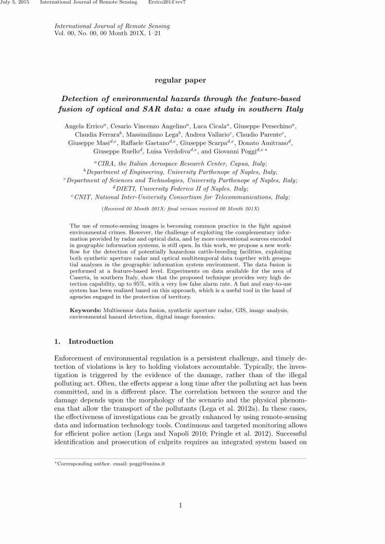
Figure 1. RGB composite of one of the available optical images. The area is about 14 × 12 km2 with aspatial resolution of 2 m/pixel for the multispectral bands and 0.5 m/pixel for the panchromatic band.

(Blue, Green, Red, Near-Infrared) co-registered with the panchromatic band butwith a geometric resolution of 2 m/pixel. Radiometric resolution is 8 bits for alldata. Figure 1 shows the RGB composite of the 2010-07-29 image.

2.3.2 SAR images

A set of 15 COSMO-SkyMed single-look complex balanced stripmap SAR imagesis available for the project, unevenly spanning a temporal interval of two years,between December 14, 2009, and October 17, 2011. All the data are HH polarized,acquired with ascending orbit and look angle of approximately 33o. The data coveran area of about 40 × 40 km2, with 3 m/pixel spatial resolution (both in rangeand azimuth). A calibration set for correcting the effects related to the sensor andthe acquisition geometry can be extracted from the ancillary data provided by theItalian Space Agency (ASI). In such way, the achievable radiometric accuracy isabout 1 dB. A cut of 5200 × 4600 pixels was used for the proposed project, coveringan area of about 195 km2. Figure 2 shows one of the available SAR images, geocodedand resampled on a map grid of 0.5 m/pixel (for comparison with the pansharpenedoptical image) after the application of the multitemporal De Grandi filter (DeGrandi et al. 1997), followed by a spatial non-local filter (Parrilli et al. 2012).Multitemporal filtering, by exploiting time diversity, helps in reducing speckle andhence improves the performance of the successive segmentation step (Gaetano et al.2014a). In particular, the De Grandi filter is relatively simple and has proved veryeffective in the context of several different applications (Ali et al. 2013; Amitranoet al. 2014; Fontanelli et al. 2014). The subsequent non-local filter exploits spatialdependencies to further reduce speckle, while preserving relevant image structures,as shown in Deledalle et al. (2014).

5


Figure 2. One of the available SAR images in amplitude format. The area is about 14 × 12 km2 with aspatial resolution of 3 m/pixel.

Figure 3. Optical (RGB) and SAR (amplitude) images of a selected region of interest (about 337 × 226m2) with several BBFs.

3. Proposed approach

There are probably many ways to combine and exploit the available data to detectsmall BBFs. In the following, we describe a simple processing chain, based on somepreliminary observations on the characteristics of these facilities.

As recorded from the satellite, see Figure 3, BBFs are mainly characterized bythe adjacent sheds and fenced uncovered spaces used for both breeding the buffaloand accumulating animal waste. Sheds are clearly visible in both optical images,where they have a saturated response due to their high reflectivity, and the SARimages, where they contribute bright lines due to double-reflection mechanisms.However, these responses are not at all specific and can be confused with otherhighly reflective covers in the optical images (e.g. bitumenized roads) and, espe-

6


1

?

Optical Images

OPTICAL

PROCESSING

?

?

SAR Images

SAR

PROCESSING

? ?

Vectorial Map

GIS-BASED DATA FUSION

?Detection Map

Figure 4. High-level processing chain.

cially, with generic buildings in both sources. Moreover, as mentioned above, shedsare not always close to the fenced spaces where the buffalo live. Conversely, thespectral signature of the manure is highly characteristic, easily discriminated frombare ground in the NIR band, and stable to changes in solar illumination. Needlessto say, manure is always present and abundant where the animals live, and indoorbreeding is not an acceptable option in the highly standardized buffalo-breedingprotocol for the “Mozzarella di Bufala Campana” industry. Therefore, we decidedto use GeoEye-1 optical images as main source of information, focusing on themanure signature.

In SAR images, manure does not exhibit a distinctive backscatter. However, weuse the SAR stack to detect and mask built-up areas, thus reducing false alarms.This is especially valuable since most false alarms are related to shadows projectedby buildings over bare soil, which abound in urban areas due to the high densityof buildings.

In Figure 4 we show a high-level block diagram of the proposed workflow. Severaloptical images available at different dates are processed independently to generatemaps of candidate BBFs. The whole multi-temporal SAR stack is instead processedjointly to produce the built-up areas mask. These outputs are then converted in avectorial form and processed in the GIS environment, together with the cadastralmap including prior information on the location of facilities officially registered.The final product is a map of likely BBFs unknown to the official registry, whichcan be used in turn as input for on-site inspections by the environment protectionand law enforcement agencies.

In Figure 5 we show finer details for the optical and SAR processing chains. Themain goal of optical image processing is classification: based on their properties,pixels are labeled as either “manure” or “not manure”. To improve performanceand reduce complexity, classification is carried out on homogeneous image segmentsrather than isolated pixels. Therefore, after a preliminary pansharpening, the imageis segmented, in order to identify its elementary homogeneous regions. Each high-resolution segment is then characterized by its spectral signature and classified.

The SAR image processing block, instead, provides a map of the urban areas inthe scene. This is obtained by first co-registering the SAR images to a commonmaster, and then computing the stack of corresponding coherence maps which isthresholded to provide the desired urban mask.

In the data fusion block (see Figure 4), after geo-referencing and co-registering

7


1

Optical Image

?PANSHARPENING

?SEGMENTATION

?CLASSIFICATION

?Classification Map

SAR Images

?COREGISTRATION

?COHERENCE

?THRESHOLDING

?Urban Mask

Figure 5. Optical-domain and SAR-domain detailed processing chain.

all products, the classification maps corresponding to the various dates (two in ourcase) are combined through a logical AND, discarding in advance, however, regionstoo small and isolated. Detections occurring in urban areas, singled out thanks tothe SAR-domain processing, are removed as well. The resulting map, convertedfrom raster to vectorial form, is eventually compared with the cadastral map to findsuspect BBFs. Despite its simplicity, this workflow turns out to be quite effective,as shown in Section 7, and easily manageable by nonexpert users, as the operatorsof governmental agencies may be expected to be. In fact, the output BBFs mapcan be obtained and updated with a small number of simple operations, makingthe human-machine interaction experience quick and comfortable, thus orientedtowards the end-users community (Madhok and Landgrebe 2002; Gaetano et al.2014a; Amitrano et al. 2015).

4. Optical-domain Image Processing

The first task carried out on the multiresolution images is pan-sharpening, whichprovides a data cube with full spatial and spectral resolution. We resort here tothe Gram-Schmidt method, which has become very popular for pan-sharpening(Laben and Brower 200) due to its good performance over a wide variety of ap-plications (Du et al. 2007; Yusuf et al. 2012). Moreover, it is implemented in theENVI package, one of the most commonly used commercial software packages forthe processing of remote-sensing images. In the following, the segmentation andclassification processing are discussed.

4.1 Segmentation

Remote-sensing images come in the form of arrays of pixels, hardly a good basison which to make reliable decisions. Therefore, it is convenient to raise the descrip-tion to a higher level, by identifying elementary regions, or segments, which areinternally homogeneous, and hence characterized by means of a few compact fea-tures. These are, however, large enough to simplify all subsequent processing andenable the fast and reliable achievement of all application goals. This processingparadigm is also referred to as object-based image analysis (OBIA) or geospa-

8


(a) (b) (c) (d)

Figure 6. Edge Mark and Fill segmentation. (a) original RGB clip (about 540 × 200 m2), (b) watershedsegmentation map, (c) morphological and spectral markers, (d) EMF segmentation map.

tial OBIA (GEOBIA), and is widely adopted as shown in the review proposed inBlaschke (2010).

In the present study, given the need to extract region contours as accuratelyas possible for subsequent vectorization, we resort to edge-oriented segmentationtechniques based on the watershed transform. First, we compute the map of imageedges on the high-resolution panchromatic component.

However, the application of watershed to real-world remote sensing images, seeFigure 6(a), provides an exceedingly large number of regions, Figure 6(b), manyof which are due to minor imperfections of the edge map, or just to the discretegeometry of the images and should be obviously merged together. We thereforeapply a more sophisticated segmentation algorithm, called Edge Mark and Fill(EMF), proposed originally in (Gaetano et al. 2012) and generalized in (Gaetanoet al. 2014b) for color and multiresolution images. Edge detection is here performedusing the Canny edge detector (Canny 1986), which is largely available and flexibleand has been proven to perform well within the EMF framework.

EMF carries out a marker-controlled watershed segmentation. Markers are re-gions superimposed to the original image that force all pixels covered by a givenmark to belong to the same segment. They can be put manually by an operator, atedious and low-precision task or, more interestingly, through some specific auto-matic procedure, e.g. (Xiao et al. 2007; Gaetano et al. 2012). In EMF, two typesof markers are automatically generated and fused, based, respectively, on the mor-phological properties of the Canny edge map, and on the spectral properties ofthe corresponding adjacent regions. In Figure 6(c), we show some of the markersgenerated by EMF, superimposed on the original image. Thanks to such markers,the final segmentation map, shown in part (d), comprises a much smaller numberof segments with the same accuracy, partially closing the gap with the ideal mapthat a human being might generate.

9


Figure 7. Training (left) and test (right) sets for classification. Red boxes correspond to “manure” areas.

4.2 Spectral Classification

Our aim is to classify each segment of the area of interest as either “manure” or“not manure”, based on the spectral response vectors of the component pixels,obtained through the pansharpening of the multiresolution optical image. To thisend, given the wealth of information available, we resort to supervised classification.

The spectral response of “manure” cannot be discriminated from that of othersemantic classes, and hence a more general “wet soil” class was used with regard toclassification. As discussed in the following, “manure” can be discriminated withrespect to other land covers of the “wet soil” spectral class only by going beyondspectral analysis. The proposed model eventually comprises 15 classes (see Table2), including for example “green vegetation”, “dry vegetation”, and “bare soil”.For our purposes, however, all segments not classified as “wet soil” are eventuallycollected in a single class and discarded from further analysis.

A relatively small fraction of the image was selected as the training set, takingcare to include all the features of interest. More precisely, for each class of interest,we selected from 20 to 50 segments each comprising a few hundreds pixels, exceptfor some classes of particularly small objects, such as clay, asphalt, green roofs,and trees. In fact for these classes smaller ground truth segments are needed (fewerthan 100 pixels) for reliable annotation. Overall, about 200,000 pixels were usedfor the training set. In the same manner, we formed a test set of approximately110,000 pixels, taking care to avoid any intersection between training set and testset segments. Figure 7(a) shows some “wet soil” training set segments (to avoidcluttering the figure, segments of other classes are not shown), while Figure 7(b)shows some test set segments of the same class.

Given this detailed 15-class model, it is reasonable to characterize each classc = 1, . . . , C through a single-mode probability density function (pdf), and inparticular, a multivariate Gaussian with mean µc and covariance matrix Σc. Thesesynthetic statistics are maximum-likelihood estimated based on the training data,with high reliability, given the low-dimensionality (four) of the vector space, muchsmaller than the number of available pixels per class.

Given the spectral vector X(s) = x associated with pixel s, the label or classc(s) ∈ C = 1, 2, . . . , C is chosen according to the MAP (Maximum A-posterioriProbability) rule. However, lacking any prior information on the classes, this re-duces to the maximum likelihood rule, and eventually, for the assumed Gaussianstatistics, to

c(s) = arg minc∈C

[ln |Σc|+ (x− µc)TΣc

−1(x− µc)]

(1)

10


To reduce the influence of noise, the decision is made on segments, rather thanpixels. For each homogeneous region singled out by segmentation, the average spec-tral signature is computed and used for classification. Segmentation granularity iskept high in order to preserve the homogeneity of the spectral response in the samesegment. As a consequence, the physical objects of the scene are often composedby several segments. Because of the use of segments rather than pixels, the classifi-cation appears to be fairly reliable, despite the simple multivariate Gaussian modeladopted.

5. SAR-domain Image Processing

The goal of SAR-domain processing is to extract a pixel-based map of urban ar-eas, through the analysis of interferometric coherence. To this end, SAR imagesare preliminarily coregistered with one-another by a three-step procedure (Li andBethel 2008) during which the alignment is progressively refined, first using or-bit information, then the cross-correlation between coupled windows, and finallyoptimizing results with Powell’s method.

Man-made areas can be separated from natural ones based on the interferomet-ric coherence between successive acquisitions, because of their different scatteringformation physical principles (Rosen et al. 2000). Indeed, in man-made areas theback-scattering is dominated by the multiple reflections between the building ele-ments and the ground. Moreover, double and triple reflections due to the dihedralsand trihedrals are stable also with respect to variations in the observation ge-ometry (Ferretti et al. 2007). Rural areas, typically composed of trees, cultivatedfields, grasses and crops, exhibit instead back-scattering values that are stronglyinfluenced by the observation geometry as well as by changes in the scene. Thiscauses low values of interferometric coherence, especially if it is computed with alarge temporal baseline. Of course, the typical time lapse necessary to cause anappreciable fall of the coherence is different for each of the above cited objects anddepends also on the season (for example, a single rainfall can change the scenecharacteristics with a dramatic reduction of the coherence between the pre-eventand post-event images) (Franceschetti et al. 2003).

In the available dataset, the average interval between two acquisitions is in theorder of one month, which is sufficient for assuming that only stable targets (suchas buildings and roads) exhibit a high level of interferometric coherence. However,in order to minimize the probability of false alarms, a mean coherence map wasgenerated by averaging all the coherence maps between an image assumed as ref-erence and all others. Figure 8 represents the mean coherence values (left) andmap (right) of the whole SAR scene under analysis, projected onto the WGS84geographic coordinate system (north at top), where the sea has been manuallyremoved since it is irrelevant to the analysis conducted in this work. Note thatto obtain the binary map, man-made and natural areas are separated by simplethresholding (Gaetano et al. 2014a).

As a final step, we go from pixel-level to region-level maps, based on prior in-formation. Indeed, urban zones are areas of significant spatial extension with ahigh-density of man-made structures. Following this definition, we first computelocal density by averaging the pixel-level map in a circular region of radius 200 pixel(600 m) centered on the target. Then the density map is thresholded, and small(less than 10000 pixels) isolated regions are removed. Eventually, only high densitylarge regions are classified as urban areas. Figure 9 depicts the full pan-sharpeneddata set available. The highlighted portion (in yellow) overlaps the co-registered

11


Figure 8. Geocoded mean coherence map (left) and corresponding man-made mask (right). Bright pixelsindicate mostly man-made structures.

Figure 9. Dense urban areas (in lilac) extracted by refining the man-made map, superimposed on theRGB composite image.

SAR multitemporal data and is hence used in this work.

6. Data fusion

In the data fusion block, decisions are made based on all available pieces of in-formation. Before that, however, co-registration and rectification are required, inorder to provide coherent data.

6.1 Coregistration between SAR and optical images

SAR/optical image registration aims at correcting the misalignment of geocodedSAR with respect to the rectified optical images. The SAR geocoded images wereobtained via a range-Doppler mode, with a 20 m-resolution digital elevation model(DEM) for compensation of terrain-induced distortion.

Although many automatic registration techniques have been proposed in the lit-

12


erature (e.g., (Inglada and Giros 2004; Suri and Reinartz 2010; Fan et al. 2013)),their robustness is still limited. Therefore, we refined the SAR/optical alignmentwith user-defined Ground Control Points (GCPs), whose selection is time consum-ing and influenced by the operator sensitivity, but must be performed only oncefor the whole dataset.

In order to improve the accuracy of the GCPs identification in the SAR maps, amultitemporal De Grandi filter has been applied to the entire available dataset, inorder to reduce the effects of speckle without loss of spatial resolution, followed bynonlocal spatial despeckling (Parrilli et al. 2012). Then, the selection of GCPs wasbased on the identification of points that are easily recognizable and detectablein both the SAR and optical maps, despite their different geometries. Hence, thepoint candidate to be selected as GCPs should be relative to areas which arestable in amplitude (on the SAR map) and easily separable from surroundingregions (Zitova and Flusser 2003), such as road crossings, buildings, boundariesbetween homogeneous areas, or other dominant features observable in both images.

Thirty uniformly distributed GCPs were selected for building the warp poly-nomial needed to align the SAR to the optical reference image. This processingallowed an alignment in the order of pixel size, which is consistent with the projectobjectives.

6.2 Rectification based on a DEM

Often georeferencing is not sufficient to guarantee a precise spatial correspondenceamong physical regions and objects in the various images, even when DEMs areused for either orthorectification or geocoding. To improve the geometric qual-ity of the original images, rectification was applied using the rational functionmodel (RFM) (Tao and Hu 2000), adopted with success in many applications (e.g.Maglione, Parente, and Vallario (2014)). This approach requires a DEM of thewhole area and at least 39 GCPs with known image coordinates and 3D (alti-metric and planimetric) position in a geodetic-cartographic reference system. A5m×5m DEM of the region of interest was built by means of linear interpolationon vector maps at a scale of 1:5000, with 99 GCPs for the first image and 201 for thesecond. Accuracy was tested by considering the difference between the exact andestimated coordinates, by means of root mean squared error (RMSE =

√MSE).

RMSE turned out always to be below 1 m for GCPs, and slightly higher than thatfor a disjoint set of control points.

6.3 Decision

After co-registering all products, several simple decision rules can be enacted basedon the segment-level classification of optical images and on the urban mask. Inparticular, we show results obtained using only one or both of the optical imagesand with and without urban masking. When two images are used, only segmentsdetected in both are taken into account (hence, a more conservative choice). More-over, the urban mask, when used, allows one to discard segments detected in urbanareas. A more detailed description of the decision process is deferred to the nextsection, in the context of the experimental analysis.

13


7. Experimental results

Here we report results of experiments carried out to validate the proposed algo-rithm. We will analyze separately the performance of classification and detectiontasks. However, since in both cases we are eventually interested in detecting thepresence of a given target class, “manure” in classification, and “buffalo breedingfacility” in detection, we will consider always the same measures, used in two-classhypotheses tests, namely precision P and recall R, and the synthetic F1 measureF . These measures are defined, w.r.t, a generic target class T , as

P = Pr(c = T | c = T ) (2)

R = Pr(c = T | c = T ) (3)

and

F =2PR

P +R(4)

where PR denotes probability, and c and c indicate the true and selectedclass/hypothesis. A high precision indicates that when the target class is detected,the decision is very likely correct. A high recall indicates that when the target classis present, it will be very likely detected. Therefore, both measures are desired tobe large, and by tuning the classification parameters one may increase one of thembut decrease the other. A synthetic measure of performance is the F -measure,a harmonic mean of precision and recall, which is large only when one or bothindicators are rapidly reducing in value.

7.1 Classification

Our classifier is trained on pixels drawn from the training set, while the decisionis made on segments, namely on the average spectral response computed over allpixels belonging to a segment. This mixed solution was chosen after comparing per-formance with the other meaningful alternatives, where training and classificationare performed both on pixels or both on segments. Results are reported in Table 1,w.r.t. the target class “wet soil”, and are computed pixel-based irrespective of howthe decision is made. Although the performance is definitely good in all cases, theselected mixed solution guarantees an appreciable gain in precision, and thereforein the F -measure. Indeed, when decisions are made on individual pixels, the influ-ence of noise is more relevant, causing a drop in both precision and recall. In thethird case, instead, the problem is likely the limited number of segments availablefor training, which reduces the ability of the classifier to deal with outliers of otherclasses. We underline also that the pixel-based solution must be excluded not onlyfor its inferior performance, but also because we will use segments as the basis forthe detection of BBFs.

For the selected solution, we computed the complete 15-class confusion matrixA over a total of N=113367 pixels, with entries aij counting the number of pixelsof class j that have been classified as belonging to class i. Based on a confusionmatrix, several global quality indicators are usually computed. The overall accuracy

14


training classification precision recall F-measure

pixel pixel 0.862 0.975 0.915

pixel segment 0.902 0.995 0.946

segment segment 0.854 0.994 0.919

Table 1. Comparison of training/cassification combinations.

τ , defined as

τ =∑i

aii/N (5)

is the percentage of sample pixels that are correctly classified. The Kappa param-eter, defined as

κ =N∑

i aii −∑

i ai+a+i

N2 −∑

i ai+a+i(6)

with ai+ =∑

j aij and a+i =∑

j aji, discounts successes obtained by chance,

and is therefore more conservative (it can be also negative). The average accuracy(AA), also frequently used, is defined as the mean of per-class producer’s accuraciesaii/a+i. Finally, the normalized accuracy τnorm is computed on a confusion matrixmodified as described in Congalton (1991) in order to give equal importance to allclasses, irrespective of the number of samples in each one. These indexes are all veryhigh for our classifier: τ = 78.19%, κ = 76.05%, AA = 80.98%, τnorm = 86.92%,especially considering the large number of classes considered, some of which prettysimilar to one another.

1 2 3 4 5 6 7 8 9 10 11 12 13 14 15 Σ

1 9712 2502 89 1233

2 42 4764 4806

3 76 86 1450 4 71 174 541 982 16 3400

4 4 8 3 593 2 610

5 62 4788 3 6 10 163 5432

6 18 9779 311 3 311 161 35 10618

7 79 3026 3105

8 5 1 1991 402 2399

9 609 15191 9 848 1 16658

10 1203 5 17 542 7203 2 11 8983

11 265 14 41 57 3 18 1402 616 47 42 2505

12 433 14417 17 14867

13 60 4214 574 4848

14 18 165 6 159 130 109 153 11199 67 12006

15 5 48 144 49 2 10939 11187

Σ 10532 7360 3471 593 4886 25511 3512 2058 2251 8538 1550 14586 5000 11820 11659

Table 2. 15-class confusion matrix. Labels: 1=Shallow Water, 2=Deep Water, 3=Asphalt, 4=Pools,5=Rock, 6=Bare Soil, 7=Wet Soil, 8=Clay Roofs, 9=Asphalt Roofs, 10=Metal Roofs, 11=Green Roofs,12=Trees, 13=Grass, 14=Sparse Vegetation, 15=Dry Vegetation.

In Table 2 we report the confusion matrix. With perfect classification, only di-

15


Figure 10. The image used in the experiments. Performance is computed on the large region in the yellowbox. The small region in the red box is used for detailed visual inspection of results.

Figure 11. Segment-level decisions on the same small area of the image at the two dates. Green=correct,red: false alarm.

agonal entries should be larger than 0, and indeed, most off-diagonal entries are0 (blank) or very close to it. In any case, we are especially interested in the “wetsoil” class, number 7, including “manure”, for which both producer’s and user’saccuracy are clearly very high.

7.2 Detection

Detection performance is assessed on a large part of the available image, shown inthe yellow box of Figure 10, while the small region in the red box will be used onlyfor visual inspection. Measuring performance is less obvious in this case. Our goalis to detect BBFs, when present, and to avoid declaring their presence otherwise.First, to measure success in the first task, we need a ground truth which identifiesall such facilities in the test area. Therefore, an expert photointerpreter (the firstauthor of this work) analyzed thoroughly the whole image and, based also on othercomplementary sources of information, detected eventually 76 BBFs, drawing theirapproximate contours in GIS as regular polygons, shown in yellow (nine of them)in the example clip of Figure 11.

This figure also shows the segments classified as “wet soil”, in green (correctdecision) when more than 50% of the segment is inside a BBF, or in red (false

16


variant images urban mask precision recall F-measure

1 T1 0.973 0.154 0.266

2 T1 NO 0.986 0.234 0.379

3 T1 + T2 0.934 0.862 0.897

4 T1 0.973 0.272 0.425

5 T1 YES 0.986 0.426 0.596

6 T1 + T2 0.934 0.949 0.941

Table 3. Detection performance with different variants of the proposed procedure.

alarm) otherwise. However, we are interested in detecting facilities, not segments.Therefore, we use these data to label the 76 BBFs as either detected (when com-prising at least one green segment) or missed (when no green segment falls withinits bounding polygon). In the example clip, all nine BBFs are detected at bothdates. With this information, we can compute a meaningful recall indicator. Inregard to precision, no similar conversion seems possible. So we are forced to op-erate at segment level, computing precision as the ratio between the number ofsegments (green) correctly declared “wet soil”, possibly manure, and the numberof all segments (green or red) declared “wet soil”, irrespective of their real class,thus including errors. Although working at segment level, this latter indicator pro-vides a good insight into the quality of the whole procedure. If precision is toolow, the technique indicates many more targets than actually present, becomingbasically useless. To reduce false alarms we resort to the urban mask of Figure 9,computed from the SAR coherence map.

In Table 3 we report the performance indicators obtained using all pieces ofinformation available (last row) or just some of them. In the first two cases, onlyone of the optical images is used, either T1 or T2. In both cases almost all BBFsare detected (high precision), but also thousands of “manure” regions unrelatedwith BBFs (low recall) resulting in an acceptable overall performance, as testifiedby the very low F -measure value. This was to be expected from the analysis ofFigure 11, where many red segments appear. However, while regions in BBFs arepersistent, because they are continuously covered by manure, external regions areonly occasionally classified as such, maybe because periodically fertilized, and canbe eliminated through a multitemporal analysis. By combining the maps relative toboth time instances through a simple logical AND (case 3), a much better recall isobtained. However, although not in the example clip, some BBFs are lost due to thelogical AND, reducing slightly precision. Despite this loss a much higher F -measureis observed. Figure 12 shows the effects of the logical AND on our example clip. Inthe last three rows of the table we report the same data as before when the maskfor dense urban areas, derived from SAR images, is also used. This mask allowsus to reject a number of bare soil areas that, when shadowed by buildings, arespectrally indistinguishable by wet soil, generating a large number of false alarms.Therefore, recall increases significantly with respect to the corresponding caseswithout urban mask, while precision is obviously not affected by masking, becauseBBFs are always rather far from large urban centers. The full fledged technique(case 6) guarantees eventually both high precision, with 71 facilities detected outof 76, and high recall, with only 30 false alarm segments out of 590.

17


Figure 12. Segment-level decisions based on multitemporal data. No false alarm occurs in the clip.

8. Conclusions and future research

We have proposed a methodology for detecting small buffalo-breeding facilitiesbased on multi-sensor and multitemporal remote-sensing data and GIS-based pro-cessing. The performance of the proposed system is quite satisfactory with anF -measure always above 0.9. Hence, it can be a valuable tool for monitoring envi-ronmental hazards, adaptable to different tasks by modifying the input data, andalso in regard to various highly data-dependent processing tasks, such as denoisingor segmentation. For example, work is under way to adapt the tool to the detectillegal landfill.

Of course, there is room for further improvement under several points of view.First of all, with more images available, a better decision strategy could be im-plemented, so as to detect all areas of interest with limited false alarms. However,even with the data currently available, performance could be improved by betterexploiting information available in the GIS, such as the position of candidate areasw.r.t. the road network and waterways, or other geographic layers coming fromdifferent sources. Work is currently under way to investigate these issues.

References

Ali, I., C. Schuster, M. Zebisch, M. Forster, B. Kleinschmit, and C. Notarnicola. 2013.“First Results of Monitoring Nature Conservation Sites in Alpine Region by Using VeryHigh Resolution (VHR) X-Band SAR Data.” IEEE Journal of Selected Topics in AppliedEarth Observations and Remote Sensing 6 (5): 2265–2274.

Amitrano, D., G. Di Martino, A. Iodice, D. Riccio, and G. Ruello. 2015. “A new frame-work for SAR multitemporal data RGB representation: rationale and products.” IEEETransactions on Geoscience and Remote Sensing 53 (1): 117–133.

18


Amitrano, D., G. Di Martino, A. Iodice, D. Riccio, G. Ruello, F. Ciervo, M. N. Papa,and Y. Koussoube. 2014. “Effectiveness of High-Resolution SAR for Water ResourceManagement in Low-Income Semi-Arid Countries.” International Journal of RemoteSensing 35 (1): 70–88.

Barba, M., A. Mazza, C. Guerriero, M. Di Maio, F. Romeo, P. Maranta, I. Marino, M. G.Paggi, and A. Giordano. 2011. “Wasting Lives: The Effects of Toxic Waste Exposureon Health. the Case of Campania, Southern Italy.” Cancer Biology & Therapy 12 (2):106–111.

Blaschke, T. 2010. “Object based image analysis for remote sensing.” ISPRS Journal ofPhotogrammetry and Remote Sensing 65 (1): 2–16.

Brilis, G.M., R.J. van Waasbergen, P.M. Stokely, and C.L. Gerlach. 2001. “Remote sensingtools assist in environmental forensics: Part II - Digital Tools.” Environmental Forensics2 (3): 223 – 229.

Canny, J. 1986. “A Computational approach to edge detection.” IEEE Transactions onPattern Analysis and Machine Intelligence 8 (6): 679–698.

Congalton, R. G. 1991. “A Review of Assessing the Accuracy of Classifications of RemotelySensed Data.” Remote Sensing of Environment 37 (1): 35–46.

De Grandi, G. F., M. Laysen, J.-S. Lee, and D. Schuler. 1997. “Radar reflectivity estimationusing multiple SAR scenes of the same target: technique and applications.” In IEEEInternational Geoscience and Remote Sensing Symposium, 1047–1050. August.

Deledalle, C.-A., L. Denis, G. Poggi, F. Tupin, , and L. Verdoliva. 2014. “Exploiting PatchSimilarity for SAR Image Processing: The Nonlocal Paradigm.” IEEE Signal ProcessingMagazine 31 (4): 69–78.

Du, Q., N. H. Younan, R. King, , and V. P. Shah. 2007. “On the Performance Evaluationof Pan-Sharpening Techniques.” IEEE Geoscience and Remote Sensing Letters 4 (4):518–522.

EPA, U.S. 2011. “National pollutant discharge elimination system (NPDES) concentratedanimal feeding operation (CAFO) reporting rule.” .

Esposito, M., F. P. Serpe, F. Neugebauer, S. Cavallo, P. Gallo, G. Colarusso, L. Baldi,G. Iovane, and L. Serpe. 2010. “Contamination Levels and Congener Distribution ofPCDDs, PCDFs and Dioxin-Like PCBs in Buffalo’s Milk from Caserta Province (Italy).”Chemosphere 79 (3): 341–348.

Faisal, K., M. Alahmad, and A. Shake. 2012. “Remote Sensing Techniques as a tool forEnvironmental Monitoring.” In International Archives of the Photogrammetry, RemoteSensing and Spatial Iinformation Sciences (XXII ISPRS Congress), 513 – 518. August.

Fan, B., C. Huo, C. Pan, and Q. Kong. 2013. “Registration of optical and SAR satelliteimages by exploring the spatial relationship of the improved SIFT.” IEEE Geoscienceand Remote Sensing Letters 10 (4): 657–660.

Fatta-Kassinosa, D., I. K. Kalavrouziotisb, P. H. Koukoulakisc, and M. I. Vasqueza. 2011.“The Risks Associated with Wastewater Reuse and Xenobiotics in the AgroecologicalEnvironment.” Environmental Health Perspectives 409 (19): 3555–3563.

Ferretti, A., A. Monti-Guarnieri, C. Prati, F. Rocca, and D. Massonnet. 2007. InSARprinciples: guidelines for SAR interferometry processing and interpretation. Postbus 229,2200 AG Noordwijk: ESA Publications, ESTEC.

Fontanelli, G., A. Crema, R. Azar, D. Stroppiana, P. Villa, and M. Boschetti. 2014. “CropMapping Using Optical and SAR Multi-Temporal Seasonal Data: A Case Study in Lom-bardy Region, Italy.” In IEEE International Geoscience and Remote Sensing Sympo-sium, 1489–1492.

Franceschetti, G., A. Iodice, D. Riccio, G. Ruello, , and S. Cimmino. 2003. “SAR RawSignal Simulation for Urban Structures.” IEEE Transactions on Geoscience and RemoteSensing 41 (9): 1986–1995.

Gaetano, R., D. Amitrano, G. Masi, G. Poggi, G. Ruello, L. Verdoliva, and G. Scarpa.2014a. “Exploration of multitemporal COSMO-SkyMed data via tree-structured MRFsegmentation.” IEEE Journal of Selected Topics in Applied Earth Observations andRemote Sensing 7 (7): 2763–2775.

Gaetano, R., G. Masi, G. Poggi, L. Verdoliva, and G. Scarpa. 2014b. “Marker controlled

19


watershed based segmentation of multi-resolution remote sensing images.” IEEE Trans-actions on Geoscience and Remote Sensing in press.

Gaetano, R., G. Masi, G. Scarpa, and G. Poggi. 2012. “A marker-controlled watershed seg-mentation: Edge, mark and fill.” In IEEE International Geoscience and Remote SensingSymposium, 4315–4318. july.

Gao, M., S. Liu, Z. Qin, J. Qiu, B. Xu, W. Li, X. Yang, and J. Li. 2013. “Integrationof remote sensing with GIS for grassland snow cover monitoring and snow disasterevaluating in Tibet.” In proc. of SPIE, Remote Sensing for Environmental Monitoring,GIS Applications, and Geology VIII, Vol. 7110October.

Gerba, C. P., and J. E. Smith. 2005. “Sources of Pathogenic Microorganisms and TheirFate during Land Application of Wastes.” Journal of Environmental Quality 34 (1):42–48.

Horrigan, L., R. S. Lawrence, and P. Walker. 2002. “How Sustainable Agriculture CanAddress the Environmental and Human Health Harms of Industrial Agriculture.” En-vironmental Health Perspectives 10 (5): 445–456.

Im, J., J.R. Jensen, R.R. Jensen, J. Gladden, J. Waugh, and M. Serrato. 2007. “Vegetationcover analysis of hazardous waste sites in Utah and Arizona using hyperspectral remotesensing.” Remote Sensing 4: 327 – 353.

Infascelli, R., S. Faugno, S. Pindozzi, R. Pelorosso, and L. Boccia. 2010. “The Environmen-tal Impact of Buffalo Manure in Areas Specialized in Mozzarella Production, SouthernItaly.” Geospatial Health 5 (1): 131–137.

Inglada, J., and A. Giros. 2004. “On the possibility of automatic multisensor image regis-tration.” IEEE Transactions on Geoscience and Remote Sensing 42 (10): 2104–2120.

Jensen, J., M. Hodgson, M. Garcia-Quijano, J. Im, and J. Tullis. 2009. “A remote sensingand GIS-assisted spatial decision support system for hazardous waste site monitoring.”Photogrammetric Engineering and Remote Sensing 75 (2): 169 – 177.

Jongbloed, A. W., and N. P. Lenis. 1998. “Environmental Concerns about Animal Manure.”Journal of Animal Science 76 (10): 2641–2648.

Karathanassi, V., C. Choussiafis, and Z. Grammatikou. 2012. “Monitoring the change involume of waste in landfill using SAR interferometry.” In 32nd EARSel Symposium,Adavances in Geosciences, 540 – 551.

Laben, C. A., and B. V. Brower. 200. “Process for Enhancing the Spatial Resolution ofMultispectral Imagery Using Pan-Sharpening.” US Patent 6,011,875.

Lega, M., D. Ceglie, G. Persechino, C. Ferrara, and R.M.A. Napoli. 2012a. “Illegal dumpinginvestigation: A new challenge for forensic environmental engineering.” WIT Transac-tions on Ecology and the Environment 163: 3–11.

Lega, M., J. Kosmatka, C. Ferrara, F. Russo, R. M. A. Napoli, and G. Persechino. 2012b.“Using advanced aerial platforms and infrared thermography to track environmentalcontamination.” Environmental Forensics 13 (4): 332–338.

Lega, M., and R. M. A. Napoli. 2010. “Aerial infrared thermography in the surface waterscontamination monitoring.” Desalination and Water Treatment 23 (1-3): 141–151.

Lein, J.K. 2013. “Landfill monitoring using remote sensing: a case study of Glina, Roma-nia.” Waste Management and Research 31: 1075 – 1080.

Li, Z., and J. Bethel. 2008. “Image coregistration in SAR interferometry.” In The In-ternational Archives of the Photogrammetry, Remote Sensing and Spatial InformationServices, XXXVII (B1), 433–438.

Madhok, V., and D. A. Landgrebe. 2002. “A process model for remote sensing data anal-ysis.” IEEE Transactions on Geoscience and Remote Sensing 40 (3): 680–686.

Maglione, P., C. Parente, and A. Vallario. 2014. “Coastline Extraction Using High Resolu-tion WorldView-2 Satellite Imagery.” European Journal of Remote Sensing 47: 685–699.

Menzi, H., O. Oenema, C. Burton, O. Shipin, P. Gerber, T. Robinson, and G. Franceschini.2010. “Impacts of Intensive Livestock Production and Manure Management on the Envi-ronment.” In Livestock in a Changing Landscape: Drivers, Consequences and Responses,edited by H. Steinfeld, H. Mooney, L. E. Neville, and F. Schneider. Washington, DC:Island Press.

Ottavianelli, G., S. Hobbs, R. Smith, and D. Bruno. 2005. “Assessment of SAR data and

20


interferometric products for solid waste landfill management.” In RSPSoc Annual Con-ference 2005 - Measuring, Mapping and Managing a Hazardous World, 1–8. September.

Parrilli, S., M.Poderico, C.V.Angelino, and L.Verdoliva. 2012. “A nonlocal SAR image de-noising algorithm based on LLMMSE wavelet shrinkage.” IEEE Transactions on Geo-science and Remote Sensing 50 (2): 606–616.

Persechino, G., M. Lega, G. Romano, F. Gargiulo, and L. Cicala. 2013. “IDES project: Anadvanced tool to investigate illegal dumping.” WIT Transactions on Ecology and theEnvironment 173: 603–614.

Pohl, C., and J. V. Genderen. 1998. “Multisensor image fusion in remote sensing: concepts,methods and applications.” International Journal of Remote Sensing 19 (5): 823–854.

Pringle, J.K., A. Ruffell, J.R. Jervis, L. Donnelly, J. McKinley, J. Hansen, R. Morgan,D. Pirrie, and M. Harrison. 2012. “The use of geoscience methods for terrestrial forensicsearches.” Earth-Science Reviews 114: 108–123.

Rosen, P. A., S. Hensley, I. R. Joughin, F. K. Li, S. N. Madsen, E. Rodriguez, and R. M.Goldstein. 2000. “Synthetic Aperture Radar Interferometry.” Proceedings of the IEEE3 (88): 333–382.

Silvestri, S., and M. Omri. 2008. “A method for the remote sensing identification of uncon-trolled landfills: formulation and validation.” International Journal of Remote Sensing29: 975–989.

Slonecker, T., G.B. Fisher, D.P. Aiello, and B. Haack. 2010. “Visible and infrared remoteimaging of hazardous waste: a review.” Remote Sensing 2: 2474 – 2508.

Solberg, A.H.A., T. Taxt, and A.K. Jain. 1996. “A Markov random field model for classifi-cation of multisource satellite imagery.” IEEE Transactions on Geoscience and RemoteSensing 34 (1): 100–113.

Suri, S., and P. Reinartz. 2010. “Mutual-information-based registration of Terrasar-X andIkonos imagery in urban areas.” IEEE Transactions on Geoscience and Remote Sensing48 (2): 939–949.

Tao, C. V., and Y. Hu. 2000. “Image rectification using a generic sensor model - rationalfunction model.” In International Archives of Photogrammetry and Remote Sensing,Vol. XXXIII, Part B3, 874–881.

Triassi, M., R. Alfano, M. Illario, A. Nardone, O. Caporale, , and P. Montuori. 2015.“Environmental Pollution from Illegal Waste Disposal and Health Effects: A Review onthe Triangle of Death.” International Journal of Environmental Research and PublicHealth 12 (2): 1216–1236.

Waske, B., and S. van der Linden. 2008. “Classifying multilevel imagery from SAR and op-tical sensors by decision fusion.” IEEE Transactions on Geoscience and Remote Sensing46 (5): 1457–1466.

Weis, M., S. Muller, C.-E. Liedtke, and M. Pahl. 2005. “A framework for GIS and imagerydata fusion in support of cartographic updating.” Information Fusion 6 (4): 311–317.

Weng, Q. 2002. “Land use change analysis in the Zhujiang Delta of China using satelliteremote sensing, GIS and stochastic modelling.” Journal of Environmental Management64: 273–284.

Xiao, P., X. Feng, S. Zhao, and J. She. 2007. “Multispectral IKONOS image segmentationbased on texture marker-controlled watershed algorithm.” In Proc. SPIE: Remote Sens-ing and GIS Data Processing and Applications; and Innovative Multispectral Technologyand Applications, Vol. 6790.

Yusuf, Y., I. Alimuddin, J. T. S. Sumantyo, , and H. Kuze. 2012. “Assessment of Pan-Sharpening Methods Applied to Image Fusion of Remotely Sensed Multi-Band Data.”International Journal of Applied Earth Observation and Geoinformation 18: 165–175.

Zhang, J. 2010. “Multi-source remote sensing data fusion: status and trends.” InternationalJournal of Image and Data Fusion 1 (1): 5–24.

Zitova, B., and J. Flusser. 2003. “Image registration methods: a survey.” Image and VisionComputing 21 (11): 977–1000.

21

regular paper - unina.itwpage.unina.it/donato.amitrano/publications/journals/2015_ijrs... · bbfs....

Documents