regularities in sequential decision-making problemsszepesva/thesis/farahmand11.thesis.pdf · 2...

Regularities in SequentialDecision-Making Problems

Amir massoud Farahmand

1

Contents

1 Introduction 51.1 Agent Design as a Sequential Decision Making Problem . . . 51.2 Regularities and Adaptive Algorithms . . . . . . . . . . . . . 71.3 Contributions . . . . . . . . . . . . . . . . . . . . . . . . . . 91.4 Research Plan . . . . . . . . . . . . . . . . . . . . . . . . . . 121.5 Credits . . . . . . . . . . . . . . . . . . . . . . . . . . . . . . 14

2 Sequential Decision-Making Problems 152.1 Definitions . . . . . . . . . . . . . . . . . . . . . . . . . . . . 152.2 Reinforcement Learning and Planning . . . . . . . . . . . . . 212.3 Value-based Approaches for Reinforcement Learning and Plan-

ning . . . . . . . . . . . . . . . . . . . . . . . . . . . . . . . 242.4 Performance Measures . . . . . . . . . . . . . . . . . . . . . 272.5 Reinforcement Learning and Planning in Large State Spaces 282.6 Concentrability of Future-State Distribution in MDPs . . . . 33

3 Regularized Fitted Q-Iteration 373.1 Introduction . . . . . . . . . . . . . . . . . . . . . . . . . . . 373.2 Algorithm . . . . . . . . . . . . . . . . . . . . . . . . . . . . 393.3 Error Propagation . . . . . . . . . . . . . . . . . . . . . . . 433.4 Finite-Sample Convergence Analysis for RFQI . . . . . . . . 443.5 Sparsity Regularities and l1 Regularization . . . . . . . . . . 473.6 Model Selection for Regularized Fitted Q-Iteration . . . . . 483.7 Related Works . . . . . . . . . . . . . . . . . . . . . . . . . . 49

4 Regularized Policy Iteration 514.1 Main Idea . . . . . . . . . . . . . . . . . . . . . . . . . . . . 514.2 Approximate Policy Evaluation . . . . . . . . . . . . . . . . 524.3 Regularized Policy Iteration Algorithms . . . . . . . . . . . . 574.4 Finite-Sample Convergence Analysis for REG-BRM and REG-

LSTD . . . . . . . . . . . . . . . . . . . . . . . . . . . . . . 61

2

4.5 l1-Regularized Policy Iteration . . . . . . . . . . . . . . . . . 654.6 Related Works . . . . . . . . . . . . . . . . . . . . . . . . . . 66

5 Model Selection 695.1 Complexity Regularization . . . . . . . . . . . . . . . . . . . 725.2 Cross-Validation Methods . . . . . . . . . . . . . . . . . . . 745.3 Dynamical System Learning for Model Selection . . . . . . . 745.4 Functional Estimation under Distribution Mismatch . . . . . 75

A Supervised Learning 79A.1 Regression Problem . . . . . . . . . . . . . . . . . . . . . . . 80A.2 Lower Bounds for Regression . . . . . . . . . . . . . . . . . . 81A.3 On Regularities . . . . . . . . . . . . . . . . . . . . . . . . . 83A.4 Algorithms for Regression Problems . . . . . . . . . . . . . . 85

B Mathematical Background 91

Bibliography 95

Abstract

Solving a sequential decision-making problem with a large state space can beextremely difficult unless one is to benefit from the intrinsic regularities of theproblem. Such regularities might be the smoothness or the sparsity of the truevalue function or the closeness of input data to a low-dimensional manifold.

The goal of this research is to develop and analyze algorithms that adapt tothe actual difficulty of the problem. We investigate nonparametric value estima-tion methods that use regularization to control the complexity of solutions.

In this research, we develop Regularized Fitted Q-Iteration (an approximatevalue iteration algorithm) and Regularized Least-Squares Temporal Differenceand Regularized Bellman Residual Minimization (as the policy evaluation pro-cedure for approximate policy iteration algorithm), and prove their finite-sampleerror bounds. Our analyses show that the proposed algorithms enjoy an almostoptimal error convergence bound.

Finally, we discuss the model selection in sequential decision-making prob-lems, and show that it has intrinsic difficulties which make it quite different fromconventional supervised learning settings.

September 8, 2009 3

Chapter 1

Introduction

1.1 Agent Design as a Sequential Decision

Making Problem

Many real-world decision-making problems are in fact instances of sequen-tial decision-making problems. In most cases, these problems, that can bedescribed in Reinforcement Learning (RL) or Planning settings, con-sist of large state spaces that conventional solution methods cannot handleefficiently1,2. The goal of this proposal is to introduce flexible and efficientmethods for solving these problems.

We use the following example to show how one may face a large sequen-tial decision-making problem in a robotic application. Nevertheless, we donot focus on any specific application domain later, and our emphasize willbe more on theoretical studies.

The Household Humanoid

Imagine a humanoid robot (Kemp et al. [2008]) that is responsible for run-ning a household (Prassler and Kosuge [2008]) and is making meaningfulsocial interactions with humans (Breazeal et al. [2008]). The robot cansense the external world (Christensen and Hager [2008]) through its stereo-vision cameras (Daniilidis and Eklundh [2008]; Chaumette and Hutchinson

1We define state space and other related definitions in Chapter 2.2Even though we have tried to provide a self-contained technical document, there

might be places where some background knowledge from statistical machine learningand reinforcement learning/planning are required. The knowledge of machine learningalgorithms at the level of Hastie et al. [2001], statistical learning theory at the level ofGyorfi et al. [2002], and reinforcement learning/approximate dynamic programming atthe level of Bertsekas and Tsitsiklis [1996] should suffice in most cases.

5

1. Introduction

[2008]), microphones, and tactile sensors (Cutkosky et al. [2008]) all aroundits body. Moreover, in order to handle delicate tasks such as grasping (Mel-chiorri and Kaneko [2008]; Prattichizzo and Trinkle [2008]) dishes and usingstairs, it has a motor-rich body with tens of degrees of freedom. The goalof the designer is to develop an ”artificial mind” (or a decision-maker) thatperceives sensory inputs, and provides appropriate motor commands so thatthe robot can successfully complete the required tasks.

Two extremely different approaches to have such an artificial mind iseither to hand-design the decision-maker with all of its details, or to let therobot automatically find the artificial mind from scratch.

Hand-designing all aspects of this delicate decision-maker can be ex-tremely difficult. On the one hand, the designer observes the world differ-ently from the robot. There is then an intrinsic difficulty in transferring thedesigner’s knowledge to the robot, which can be further complicated withthe problem that a designer does not necessarily have sufficiently-detailedknowledge about the way he solves his everyday problems.

On the other hand, the robot’s environment, the house, changes every-day. In order to have a robust decision-maker that performs reasonably wellunder a large variety of circumstances, the designer should either predictthe situation or design an adaptation mechanism for the robot that altersits decision-maker appropriately. Designing a reactive controller that canperform well under all possible situations is difficult as it requires foreseeingall possible situations, which is impractical in unstructured environments.

The alternative is to automate the design process to an extent that theagent would ”adapt” to new situations. One extreme way is as limited asvarying a few internal variables based on observed data. The other extremeis arguably to automate the design of the whole morphology, which is theshape and structure of the body including the type and placement of sensorsand actuators, and artificial mind of the robot.

One way to see the design problem is to cast it as an appropriate opti-mization problem and to find an acceptable-enough solution for it througha learning or evolution process. Many research papers and books havebeen published on different aspects of learning or evolution for designingintelligent agents such as robots, and any attempt to summarize them inthis short space is futile. Instead, we refer the reader to Kortenkamp andSimmons [2008]; Mataric and Michaud [2008]; Billard et al. [2008]; Meyerand Guillot [2008]; Floreano et al. [2008]; Farahmand et al. [2009c] andthe references therein for more information about different approaches ofrobot programming, and the relation between learning and evolution in thiscontext.

The aforementioned robotic problem is an instance of sequential decision-

6 September 8, 2009

Regularities and Adaptive Algorithms

making problems. It is sequential because many tasks, like preparing meal,have a temporal aspect and achieving them requires a planned sequenceof actions ahead of time. The robot also requires to deal with large statespaces. Consider the robot’s sensory inputs like its cameras that provide therobot with high-dimensional real-valued inputs. The decision-maker maysummarize all these sensory inputs in an internal representation, which weinformally call state, and base its decision on the robot’s current state. Ifthe state is expected to be a good representative of what has happened inthe external world, the size of state space is huge, especially if the exter-nal world is not so structured and its description cannot be considerablycompressed.

Humanoid robotics is indeed only an instance of sequential decision-making problems with large state spaces. Other fields of robotics, suchas visual-servoing of manipulator arms (Chaumette and Hutchinson [2008];Farahmand et al. [2007a, 2009d]), mobile robots (Siciliano and Khatib [2008,Part E]), and gait optimization, also require to solve similar problems. Moregenerally, almost all control engineering problems are instances of sequentialdecision-making problems.

Nevertheless, a theory for solving sequential decision-making problemswith large state spaces has far reaching applications. In addition to roboticsand control engineering, researchers have found this theory useful in financeand have applied it to problems such as optimized trade execution (Nevmy-vaka et al. [2006]) and to learning exercise policy for American options (Liet al. [2009]). Healthcare applications of reinforcement learning methods,and especially the dynamic treatment regime problem, are also emerging(Pineau et al. [2007]). And finally, reinforcement learning has also been usedin computer games such as backgammon (Tesauro [1994]) and Go (Silveret al. [2007]).

1.2 Regularities and Adaptive Algorithms

A natural question is to what extent one should expect a learning or plan-ning algorithm perform well for a large state-space sequential decision-making problem. Negative results from supervised learning theory suggestthat efficient learning is hopeless for some classes of problems (e.g. Theo-rem 21 in Section A.2). The situation cannot be better in RL and planningproblems, a superset of regression problems, and so it is impossible to designa universal RL/Planning method that performs well for all problems.

Fortunately, not all decision-making problems are equally difficult. Ifone finds a structure or a regularity in a given problem, one may find its

September 8, 2009 7

1. Introduction

solution with much less effort. Examples of such regularities for sequentialdecision-making problems are the smoothness of the value function, thesparsity of the value function3 in a certain basis, or the input data lying ona low-dimensional manifold (see Section A.3).

To give a concrete example when a problem has smoothness regularity,let us go back to our humanoid robot and the problem of picking up anobject with minimum control signal effort. The optimal value function,which is formally defined in Section 2.1, assigns the value or the cost offollowing the optimal sequence of actions from each state. For this taskthe state representation might be the relative position of the object to therobot and the position of the joint variables.

Consider a small change to the relative position of the object to therobot. Because the dynamics of the robot is continuous in most of the statespace (except for maybe a small subset of the whole space), and it is alsoa continuous function of the control signal, any small changes in relativeposition can be ”compensated” by a small change in the control signal.Moreover, the value function is a continuous function of the control signal –because the cost is defined as the integral of squared control signal. There-fore, a small change in the state space leads to a small change in the valuefunction. This informal argument, which of course can be formalized, showsthat the value function is a continuous function of the state. Depending onthe exact properties of the robot and the way state space is defined, onemay even show that the value function has other types of [higher-order]smoothness too.

Results from supervised learning theory ensure that whenever a problemhas some certain types of regularities, the algorithm can benefit from themand one can hope to get reasonable performance. Two key points deservea closer look. The first is that the problem itself must be regular. Forexample, the value function should be smooth, or it could be described bya few dimensions of the state space. Regularity is an intrinsic propertyof the problem. The second key point is the capability of the algorithm toexploit the regularity. For instance, even though the value function might besmooth, the K-Nearest Neighborhood-based algorithm cannot benefit fromit and the performance would be almost identical to a situation withoutthis certain smoothness regularity.

In general, a highly desirable requirement for any decision-making sys-tem and in particular the learning algorithms is their adaptation to the

3We have not defined the value function yet. This is done in Section 2.1. Readersnot familiar with value functions can read the sentence by replacing ”value function”with ”target function” in a sense that is used in the regression literature.

8 September 8, 2009

Contributions

actual difficulty of the problem. If one problem is ”more regular” thananother, in a well-defined manner, we would like the decision-making orlearning algorithm to deliver better solution(s) with the same amount ofdata samples, computation time, or storage. Such procedures are calledadaptive (Gyorfi et al. [2002]).

To clarify the issue, consider a simple numerical analysis example: theproblem of inverting a matrix. If the matrix has some special structure,like being diagonal or lower/upper triangular, the matrix inversion is com-putationally cheaper than the general case. If an algorithm detects such astructure and adjusts the inversion method accordingly, we call the algo-rithm adaptive to this structural regularity.

An adaptive procedure is typically built in two steps: (1) designing flexi-ble methods with a few tunable parameters that whenever their parametersare chosen properly can deliver optimal performance for a set of desirableregularities, and (2) designing an algorithm that tunes the parameters effi-ciently so that the algorithm in (1) is actually working in the right class ofproblems (automatic model-selection).

More information about the possible difficulty of solving a learning prob-lem and common types of regularities in the supervised learning context canbe found in Appendix A and Section A.3 in particular.

1.3 Contributions

The goal of this research is to develop flexible nonparametric value-basedalgorithms for dealing with sequential decision-making problems with largestate spaces4. The main contributions of this research are three-fold:

• Formulating the sequential decision-making problem as an optimiza-tion problem in large function spaces, and demonstrating how to solvethem.

• Devising adaptive model selection methods.

• Analyzing the statistical properties of suggested methods and provid-ing finite-sample error convergence bounds.

An adaptive learning method, which can capture different regularities of SequentialDecision-Making as anOptimizationProblem

the target value function, should flexibly work with different function spacesand must be capable of representing a large set of functions. A parametricand pre-fixed function space is not suitable because it severely limits the set

4The alternative is direct policy search algorithms, but we do not consider them here.

September 8, 2009 9

1. Introduction

of representable value functions. One way to have such a flexible methodis to work with a huge function space, such as various reproducing kernelHilbert Spaces (RKHS) or Besov spaces (through Wavelet basis) that canpotentially capture many types and amounts of regularities (e.g. from verysmooth function to rugged ones), and to carefully control the solution’scomplexity by regularization (penalization) technique. This is an in-stance of nonparametric method. Regularization gives us the opportunityto control the function space’s complexity by tuning a single parameter.

Another element of an adaptive algorithm is to have an automatic modelselection method. The model selection algorithm should find the right func-Model Selec-

tion tion spaces (such as its smoothness degree) based on observed data. Thiscombination of a nonparametric method and model selection procedureleads to an adaptive learning algorithm.

Not only do we suggest learning algorithms, but we also analyze theirFinite-SampleBounds statistical properties and prove finite-sample upper bounds for the error

between the estimated value and the true value function. These resultsboth show the sanity of the proposed algorithms, and also suggest thatthese algorithms are sample-efficient: we will argue that no other algorithmcan be more efficient in the minimax sense.

Apart from this chapter that motivates the problem, this proposal hasthree chapters with new contributions, and two others that supply thereader with necessary background in sequential decision-making problems(Chapter 2) and supervised learning problems (Appendix A).

Regularized Fitted Q-Iteration (Chapter 3)

Regularized Fitted Q-Iteration (RFQI) is a nonparametric fitted valueiteration algorithm that formulates the fitting problem at each iteration ofthe value iteration as a regularized regression problem in a large functionspace such as an RKHS. We first present results that show how the errorat each iteration is propagated (Lemma 8 in Section 3.3) and then providea finite-sample convergence bound for the error occurred at each iterationfor an RKHS-based regularization methods (Theorem 9 in Section 3.4). Ifthe function space is selected appropriately, which is the job of the modelselection procedure, these two results lead to the optimal finite-sample errorconvergence bound for RFQI in Theorem 10. Moreover, we briefly discussthe issue of using sparsity regularization, which is useful for dealing withwavelets or over-complete dictionaries, in Section 3.5.

10 September 8, 2009

Contributions

Regularized Policy Iteration (Chapter 4)

We introduce regularized extensions of standard Least-Squares Tempo-ral Difference (LSTD) and Bellman Residual Minimization (BRM)algorithms as the policy evaluation methods used for the policy iteration pro-cedure (Section 4.3). We call these methods REG-LSTD and REG-BRM.When the regularized optimization problem is defined in an RKHS, weprovide closed-form solutions for REG-LSTD and REG-BRM. Finally, wepresent the finite-sample statistical analysis of these algorithms and showthat if we have correctly chosen the right function space, they have optimalconvergence bound (Section 4.4).

Model Selection (Chapter 5)

In order to get the optimal behavior of aforementioned regularized algo-rithms, one has to work in the right function space. The choice of the rightfunction space, which is usually controlled by a few parameters, is the taskof model selection algorithm.

In Chapter 5, we discuss the differences and the intrinsic difficulties ofmodel selection for sequential decision-making problems, compared with su-pervised learning problems, and suggest complexity regularization (Sec-tion 5.1), cross-validation (Section 5.2) and a virtual-model learningapproach (Section 5.3) for model selection.

Unfortunately, model selection in reinforcement learning setting witha fixed batch of data can be intrinsically difficult. We present a negativeresult in the case of simple statistical inference under distribution mismatch(also called covariate shift) where the training and testing distributions aredifferent. Distribution mismatch may occur quite often in the reinforcementlearning setting when the behavior policy and the target policy are differentand we only have access to a fixed data-set generated by the behaviorpolicy (Section 5.4). This general result implies that there cannot be asound (a notion to be later defined precisely) model selection algorithm forRL problems that works only with a fixed batch of data without puttingrestrictions on the class of problems.

In summary, the main contribution of the thesis is to introduce severalflexible nonparametric algorithms for sequential decision-making problemswith large state-spaces. These methods are adaptive and can cope with dif-ferent types of regularities with minimum user intervention. Moreover, theproposed methods have statistical finite-sample convergence bound guaran-tees.

September 8, 2009 11

1. Introduction

Nega

tive

Resu

lt fo

r Mod

el

Sele

ctio

n (J

ourn

al)

Fall2009

Winter2010

Spring2010

Summer2010

Fall2010

Mod

el S

elec

tion

with

Co

mpl

exity

Reg

ular

izatio

n

Spar

sity

Regu

lariz

atio

n fo

r RPI

Tigh

ter E

rror P

ropa

gatio

n

RPI (

Jour

nal)

Depe

nden

t dat

a fo

r RF

QI (

Jour

nal)

Conn

ectio

ns b

etwe

en

Regu

larit

ies

and

MDP

Writ

ing

Diss

erta

tion

Defe

nce

Cand

idac

y

Figure 1.1: Tentative research timeline.

1.4 Research Plan

The research of this proposal is beyond its early stages. We therefore ac-tually report some results rather than simply suggesting future directions.Nevertheless, there remain some open problems and challenges that mustbe addressed in the future. In this section, we discuss the persisting areas ofresearch. Figure 1.1 shows the tentative research and publication timeline.

Model Selection

Our model selection chapter is still fairly under-developed (Chapter 5).Developing complexity regularization-based ideas for model selection (Sec-tion 5.1) with a batch of data is the main topic to be addressed in the study.Learning the dynamical system for model selection (Section 5.3) is anothertopic to be covered.


Research Plan

Sparsity Regularization

Up to now, we have studied L2 regularization that captures the smoothnessregularity of the target function. Nevertheless sparsity regularity, whichcan be captured by l1 regularization, deserves special attention too. Thereare, however, both computational and statistical challenges to use l1 regu-larization. This will be a topic of my future research.

Dependent Data

Current error upper bounds (Theorem 9 and Theorem 12) are derived un-der condition of i.i.d. samples. Extending these results to the scenariothat samples come from a trajectory in the state space, where consecutivesamples are dependent, is another topic of study. One can use independentblocks technique to address this issue (Yu [1994]; Doukhan [1994])

Tighter Error Propagation Results

Error propagation results (Section 2.6, Lemma 8, and Lemma 13) are ratherconservative in two senses.

The first reason of its conservatism is that the supremum over all policiesin Definition 7 does not consider that policies at the later stages of policyiteration or value iteration do not alter so much. In other words, if the valuefunction is almost converged, whenever m→∞, the policy πm is expectedto be close to the policy πm+1 in an appropriate norm. The definition,however, does not consider this.

The second reason is that in deriving error propagation bounds (Lemma 8,and Lemma 13), one uses the conservative inequality

E [f(·)g(·)] ≤ sup |f(·)|E [g(·)] ,instead of the more flexible Cauchy-Schwarz inequality

E [f(·)g(·)] ≤√

E [f(·)2] E [g(·)2].

These sources of conservatism may inspire one to derive tighter bounds.This is a topic of my future research.

Connections between Regularities and MDP Characteristics

In several places of this proposal, we have expressed the problem’s regular-ities as the regularities of its value function. One research topic is relatingthese regularities to the regularities of MDP, such as the smoothness prop-erties of the transition kernel. This may help us to re-state Condition (5)of Assumption A2 and Condition (4) of Assumption A3 more directly.


1. Introduction

1.5 Credits

I acknowledge the help and contributions of Csaba Szepesvari, MohammadGhavamzadeh, and Shie Mannor. Although I have been directly involved inmost parts of this research program, there are some results which have notbeen studied or proven by me, or to which I had only minor contributions.For the sake of completeness, however, I include them in this candidacyproposal. These results are as follows.

• Results concerning error propagation have been proven by CsabaSzepesvari and Remi Munos. Section 2.6, in its current form, hasbeen mostly written by Csaba Szepesvari and Remi Munos.

• The matrix form of Theorem 11 is derived by Mohammad Ghavamzadehand Csaba Szepesvari. I was contributing to discussions about thenew representer theorem, but I have not derived the formula myself.


Chapter 2

Sequential Decision-MakingProblems

This chapter provides the necessary background on sequential decision-making problems. There we define the mathematical framework in Sec-tion 2.1, and afterwards we introduce Reinforcement Learning (RL) and Dy-namic Programming (DP)-based planning problems in Section 2.2. Thesetwo problems are very similar except that they describe situations withdifferent prior knowledge about the problem in hand. We describe thevalue-based approach to solve reinforcement learning and planning prob-lems in Section 2.3 and briefly review methods such as Value Iteration andPolicy Iteration algorithms. Next, we discuss difficulties of solving sequen-tial decision-making problems in large state spaces where one has to usefunction approximation, and categorize different aspects of using functionapproximation for RL/Planning problems in Section 2.5.

There are several standard textbooks on RL and DP. Sutton and Barto[1998] provide an introductory textbook that covers both RL and DP, withmore emphasize on learning aspects. Sutton and Barto consider both dis-crete and continuous state spaces. Bertsekas and Tsitsiklis [1996] is a moreadvanced textbook on RL and DP that focuses on finite (but large) statespaces. Bertsekas and Shreve [1978] is an advanced monograph on DP thatprovides a treatment on general state spaces – both finite and infinite.

2.1 Definitions

Probability Space

For a measurable space Ω, with a σ-algebra FΩ, we defineM(Ω) as the setof all probability measures over FΩ. B(Ω, L) denotes the space of bounded

15

2. Sequential Decision-Making Problems

measurable functions w.r.t. (with respect to) FΩ with bound 0 < L <∞.

Markov Decision Process

A finite-action MDP is a tuple (X ,A, P,R), where X is a measurable statespace, A = a1, a2, . . . , aM is the finite set of M actions, P : X × A →M(X ) is the transition probability kernel with P (·|x, a) defining the next-state distribution upon taking action a in state x, and R(·|x, a) gives thecorresponding distribution of immediate rewards.

This definition of MDP is quite general. If X is a finite state space, weget finite MDPs. Nevertheless, X can be more general. For example, if weconsider measurable subsets of Rd (X ⊆ Rd), we get the so-called continuousstate-space MDPs. In this thesis, we usually talk about measurable subsetsof Rd, but one can think of other state spaces too, e.g. binary lattices0, 1d, space of graphs with certain number of nodes, etc.

MDPs can be seen as a formalism describing a temporal evolution of astochastic dynamical system (or a stochastic process indexed by time). Thedynamical system starts at time t = 0 with random initial X0 ∼ P0

1 where” ∼ ” in X0 ∼ P0 is a symbol showing that X0 is a sample from distributionP0. The reward at time t is Rt ∼ R(·|Xt, At). Then the next state Xt+1

comes after the current state Xt according to the transition kernel P , i.e.Xt+1 ∼ P (·|Xt, At) where At is some stochastic process. This proceduregenerates a random trajectory ξ = (X0, A0, R0, X1, A1, R1, . . .). We denotethe space of all possible trajectories as Ξ.

Policy

Definition 1 (Definition 8.2 and 9.2 of Bertsekas and Shreve [1978]). Apolicy is a sequence π = π1, π2, . . . such that for each t,

πt(at|X0, A0, X1, A1, . . . , At−1, Xt)

is a universally measurable stochastic kernel on A given X ×A× . . .A×Xsatisfying

πt(A|X0, A0, X1, A1, . . . , At−1, Xt) = 1

for every (X0, A0, X1, A1, . . . , At−1, Xt).If πt is parametrized only by Xt, π is a Markov policy. If for each t and

(X0, A0, X1, A1, . . . , At−1, Xt), πt assigns mass one to a single point in A,

1P0 is not a part of the MDP definition. When we talk about MDPs as the descriptorof temporal evolution of dynamical systems, we usually implicitly or explicitly definesthe initial state distribution, so there should be no confusion.


Definitions

π is called a deterministic (nonrandomized) policy. If π is a Markovpolicy in the form of π = (π, π, . . .), it is called a stationary policy.

Under certain conditions, it can be shown that a deterministic Markovstationary policy is all we should care for, e.g. see Proposition 4.3 of Bert-sekas and Shreve [1978]. From now on, whenever we use term ”policy”, weare referring to a deterministic Markov stationary policy and we denote itby π (instead of π).

The policy π defines a set of trajectories and induces a unique prob-ability measure on them: let X0 ∼ P0 be given, and for t = 0, 1, . . . , letXt+1 ∼ P (·|Xt, At = π(Xt)). Proposition 7.45 of Bertsekas and Shreve[1978] shows that there is a unique probability measure on the sequenceξt = (X0, A0, . . . , Xt−1, At−1) for t = 0, 1, . . . such that certain expectationis well-defined (see also Bertsekas and Shreve [1978, page 214]).

Planning and Reinforcement Learning as a Variational Problem

In a non-orthodox viewpoint, reinforcement learning and planning problemscan be seen as maximizing a functional of reward distribution R(·|x, a).

Let G : Ξ 7→ R be the return function that is defined by the designer ofthe sequential decision making problem. Let ξ(x) be a trajectory startingfrom x, and denote P π

ξ(x) as the probability measure induced by the policy

π on the space of all trajectories starting from x, Ξ(x). Define the followingfunctional:

J (x; π,R, P )def=

∫Ξ

G(ξ)dP πξ(x)(ξ).

In this viewpoint, the goal of planning and reinforcement learning isfinding a policy π∗ that maximizes this functional, i.e.

π∗(·)← supπJ (·; π,R, P ).

We call π∗ an optimal policy.

Discounted MDPs

One specific type of functionals that deserves special attention is discountedreward functional. This type of functional is important because it can modelsequential decision-making problems where the importance of the futurereward is lesser than the imminent one. Moreover, it is usually easier toanalyze.



Discounted reward functional is defined as

J (x; π,R, P )def=

∫Ξ

( ∞∑t=0

γtRt

)dP π

ξ(x)(ξ) = E

[∞∑

t=0

γtRt

]

where γ ∈ [0, 1) is the discount factor, and (R0, R1, . . . ) is a subsequence ofξ = (X0 = x, π(X0), R0, X1, π(X1), R1, . . . ), which is induced by the policyπ, with the obvious identification. In the discounted case, the return ran-dom variable is G(ξ) =

∑∞t=0 γtRt. Bertsekas and Shreve [1978, Proposition

7.45]) guarantees the well-definedness of this expectation.Tuple (X ,A, P,R, γ) is called a finite-action discounted MDP. Discounted

MDPs will be the focus of our further developments unless mentioned oth-erwise.

Value Functions

To study MDPs, two auxiliary functions are of central importance: thevalue and the action-value functions of a policy π.

Definition 2. The value function V π and the action-value function Qπ fora policy π are defined as

V π(x)def= E

[∞∑

t=0

γtRt|X0 = x

],

Qπ(x, a)def= E

[∞∑

t=0

γtRt|X0 = x, A0 = a

], (2.1)

for X0 (or (X0, A0) for the action-value function) coming from a positiveprobability distribution over X (or X ×A).

It is easy to see that for any policy π, if the absolute value of the expectedimmediate reward r(x, a) = E [R(·|x, a)] is uniformly bounded by Rmax,then the functions V π and Qπ are bounded by Vmax = Qmax = Rmax/(1−γ).

For a discounted MDP, we define the optimal value function by

V ∗(x) = supπ

V π(x) ∀x ∈ X .

Similarly the optimal action-value function is defined as

Q∗(x, a) = supπ

Qπ(x, a) ∀x ∈ X ,∀a ∈ A.


Definitions

We say that a deterministic policy π is greedy w.r.t. an action-valuefunction Q and write π = π(·; Q), if,

π(x) ∈ arg maxa∈A

Q(x, a) ∀x ∈ X .

Greedy policies are important because a greedy policy w.r.t. Q∗ is an opti-mal policy. Hence, knowing Q∗ is sufficient for behaving optimally (Propo-sition 4.3 of Bertsekas and Shreve [1978]).

Bellman Operators

Bellman [optimality] operators provide a useful way to describe and ana-lyze MDPs. They are particularly important because their fixed-points are[optimal] value functions. Proposition 4.2 of Bertsekas and Shreve [1978]shows the optimality of the fixed point of the Bellman optimal operators.Moreover, it shows the uniqueness of the fixed point for both Bellman andBellman optimality operators.

Definition 3 (Bellman Operators). The Bellman operators T π : B(X ) →B(X ) (for the value function V ) and T π : B(X ×A)→ B(X ×A) (for theaction-value function Q) for the policy π are defined as

(T πV )(x)def= r(x) + γ

∫V π(y)P (dy|x, a),

(T πQ)(x, a)def= r(x, a) + γ

∫Q(y, π(y))P (dy|x, a),

where r(x, a) = E [R(·|x, a)] and r(x) = EA∼π(x,·)[r(x, A)].

The fixed point of this operator is the [action-]value function of thepolicy π, i.e. T πQ = Q and T πV = V (Proposition 4.2(b) of Bertsekas andShreve [1978]).

Definition 4 (Bellman Optimality Operators). The Bellman optimalityoperators T ∗ : B(X )→ B(X ) and T ∗ : B(X ×A)→ B(X ×A) are definedas

(T ∗V )(x)def= max

a

r(x, a) + γ

∫V (y)P (dy|x, a)

,

(T ∗Q)(x, a)def= r(x, a) + γ

∫max

a′Q(y, a′)P (dy|x, a). (2.2)



Again, they have the same fixed-point property T ∗Q∗ = Q∗ and T ∗V ∗ =V ∗ (Proposition 4.2(a) of Bertsekas and Shreve [1978]).

Proposition 4.3 of Bertsekas and Shreve [1978] implies that the optimalvalue function can be attained by a deterministic Markov stationary policyif the action set is finite. Moreover, if the action set has certain compactnessconditions, this result can also be generalized to infinite action sets such asa compact subset of RA for some A ∈ N (Proposition 4.4 of Bertsekas andShreve [1978]).

As we argue in more detail later on, one does not usually have the luxuryof calculating the effect of Bellman operator on a value function when thestate space is large. In these situations, we use empirical counterparts ofthe Bellman [optimality] operator as defined as follows.

Definition 5 (Empirical Bellman Operators). The empirical Bellman op-erator

T π : (X0 × A0 ×R0)× (X1 × A1 ×R1), . . .→ R× R× . . .

is defined as

(T πQ)(Xt, At)def= Rt + γQ(Xt+1, π(Xt+1)),

and the empirical Bellman optimal operator

T ∗ : (X0 × A0 ×R0)× (X1 × A1 ×R1), . . .→ R× R× . . .

is defined as

(T ∗Q)(Xt, At)def= Rt + γ max

a′Q(Xt+1, a

′),

where Xt+1 ∼ P (·|Xt, At).

It is easy to see that the following proposition holds.

Proposition 6.

E[T πQ(X, A)|(X = Xt, A = At)

]= T πQ(Xt, At),

E[T ∗Q(X,A)|(X = Xt, A = At)

]= T ∗Q(Xt, At).


Reinforcement Learning and Planning

Notation

We must define a few other notation that will be used throughout thisproposal.

We use F as a subset of measurable functions X 7→ R. The exactspecification of this space will be clear from the context. We usually denoteF as the space of value functions, i.e. V ∈ F .

For a measure ν ∈M(X ), and a measurable function f ∈ F , we definethe L2(ν)-norm of f , ‖f‖ν , and its empirical counterpart ‖f‖ν,n as follows:

‖f‖2νdef=

∫X|f(x)|2dν(x), (2.3)

‖f‖2ν,n

def=

1

n

n∑t=1

f 2(Xt) , Xt ∼ ν. (2.4)

Similarly, we define FM as a subset of multi-valued measurable functionsX ×A → RM with the following identification:

FM = (f1, . . . , fM) : fi ∈ F ,∀i = 1, . . . ,M .

We use fj(x) = f(x, aj); j = 1, . . . ,M to refer to the jth component off ∈ FM . We usually denote FM as the space of action-value functions, i.e.Q ∈ FM .

For ν ∈M(X ), we generalize ‖·‖ν and ‖·‖ν,n defined in Eqs. (2.3)-(2.4)

to FM as follows

‖f‖2νdef=

1

M

M∑j=1

‖fj‖2ν , (2.5)

‖f‖2ν,n

def=

1

nM

n∑t=1

M∑j=1

IAt=ajf2j (Xt) =

1

nM

n∑t=1

f 2(Xt, At), (2.6)

where I· is the indicator function: for an event E, IE = 1 if and only ifE holds and IE = 0, otherwise.

2.2 Reinforcement Learning and Planning

Reinforcement Learning and Planning are two similar types of sequentialdecision making problems with the common goal of finding a policy π that



is equal or close to the optimal policy π∗. The difference between reinforce-ment learning and planning problems, as we will discuss shortly, is in ourprior knowledge about the MDP and the way we interact with it.

In Planning, the transition kernel P (·|X, A) and the reward distri-bution R(·|X, A) of the MDP is known. Conversely, in ReinforcementLearning, P and R are not directly accessible, but one interacts withthe MDP by selecting action At at state Xt, and getting a reward Rt ∼R(·|Xt, At) and going to the next state Xt+1 according to the transitionkernel. This results in a trajectory ξ = (X0, A0, R0, X1, A1, R1, . . .). Thismode of interaction is usually described by an agent-environment metaphorin RL community (Sutton and Barto [1998]).

There are some middle ground scenarios as well. Sometimes we dohave the luxury of knowing P (·|X, A) and R(·|X, A), but cannot computefunctionals involving them such as T πQ due to the large cardinality of X .Another situation is where we do not have access to P and R themselves,but have access to a flexible data generator that gets any X and A andreturns X ′ ∼ P (·|X,A) and R ∼ R(·|X, A). We call the problem of findinga good policy in these settings Approximate Planning.

There are several methods for solving reinforcement learning and plan-ning problems. These methods may be categorized based on the type ofexplicit representation that they maintain:

• Value Space Search

• Policy Space Search

Value-based approaches maintain an estimate Q (or V ) of the optimalvalue function Q∗ (or V ∗). The premise of value-based approaches is that byfinding an accurate enough estimate Q of the optimal action-value functionQ, the greedy policy π(·; Q) will be close to the optimal policy. Direct pol-icy search approaches, however, explicitly represent the policy function anddirectly perform the search in the policy space. The search may be guidedby the gradient information or can be in the same spirit as evolutionaryalgorithms (Baxter and Bartlett [2001]; Kakade [2001]; Ghavamzadeh andEngel [2007b]). Moreover, there are hybrid methods that explicitly repre-sent both value and policy functions (Konda and Tsitsiklis [2001]; Peterset al. [2003]; Ghavamzadeh and Engel [2007a]). In this proposal, we onlyfocus on exploiting regularities in value-based approaches.



Online vs. Offline Setting – Batch vs. IncrementalProcessing

An important aspect of any method that solves RL/Planning problems,be it through value or policy space search, is the way in which data arecollected and are processed by the algorithm. The data collection settingcan be categorized as online or offline and the data processing method canbe categorized as batch or incremental.

The online setting is when the agent (algorithm) can directly interact Online vs. Of-flinewith the environment. By the change of policy π, the agent has control over

how the data stream ξ = (X0, A0, R0, . . . ) is generated2. Here At ∼ π(·|Xt)(or similar) and π is selected by the agent. The offline setting, on the otherhand, is when the agent does not have control over how data is generated;it is, rather, provided with data set Dt = (X0, A0, R0, . . . , Xt−1, At−1, Rt−1).This data set is generated by a behavior policy πb, which has selected ac-tions according to Ak ∼ πb(·|Xk). Here, the algorithm does not choose thebehavior policy and the policy may even be unknown to it.

An algorithm can be batch or incremental. A batch algorithm processes Batch vs. In-crementalthe whole Dt, and can freely access any element of the data set at any time.

An incremental algorithm, however, starts learning whenever a new datasample is available. The computation does not directly depend on the wholedata set Dt, but only on (Xt, At, Rt) (or other variants of data samples). Ofcourse, the boundary between a batch algorithm and an incremental one isnot vividly clear. One may say an incremental algorithm is a special caseof batch algorithms when the algorithm process data in a special temporalordering.

In this work, we focus on batch algorithms that assume accessing to allinteraction data history in the form ofDt = (X0, A0, R0, . . . , Xt−1, At−1, Rt−1),with Ak ∼ πb(·|Xk). In most cases, we also assume that we are in the offlinesetting, i.e. the algorithm does not determine the sampling distribution ofDt.

The question of which of these settings is more natural depends on theproblem in hand. If all available is a collection of data Dt, and no chanceof interacting with the MDP, we are by definition in the offline setting.In this case as the batch algorithms are usually more data efficient, unlessthe computation time is limited, they are the preferred choice for dataprocessing. On the other hand, if we have direct access to the environment,either by knowing the model of MDP or accessing its generative model(as is common in planning) or when the agent is actually situated in the

2Later in the following chapters, we use Dn instead of Dt with an indexing schemethat starts from X1 instead of X0. The reason is merely for notational convenience.



environment, the situation is indeed online and both batch and incrementalalgorithms may be used.

Although it is customary to use incremental algorithms in the onlinesetting, batch algorithms can be and have been used in the online settingas well. The simplest way to use a batch algorithm in the online setting isto apply the algorithm at each time-step t on data Dt as if we are solving acompletely new sequential decision-making problem. Indeed, this approachis not computationally cheap. The more feasible way is that by carefulreformulation, to perform batch computation incrementally, either exactlyor approximately. For instance, matrix inversion, which is often used in thebatch computations, can be converted to an incremental computation bythe use of matrix inversion lemma. See the work of Geramifard et al. [2007]for such an attempt in RL context. There are also some algorithms to useonline learning techniques to solve problems that are usually considered asbeing in the batch setting. For instance, the work of Kivinen et al. [2004]uses stochastic gradient descent to solve optimization problems defined inan RKHS. Nevertheless, we disregard the computational aspects of ouralgorithms, and postpone them to the future work.

2.3 Value-based Approaches for


In value-based approaches for solving RL and planning problems, we aimto find the fixed point of the Bellman operator Qπ = T πQπ (for the so-called policy evaluation problem) or the Bellman optimality operatorQ = T ∗Q.3 To find the close to optimal value function, we are facing thefollowing challenges:

1. How to represent the action-value function Q?

2. Given Q, how to evaluate T πQ or T ∗Q?

3. How to find the fixed point of T π or T ∗ operators?

The first problem is easy when X and A are finite spaces, so Q canbe represented by a finite number of real values. When they are not, orhave large cardinality, we must approximate Q with simpler and easierto compute functions. This function is called approximant. The processof approximating a function with an easier to compute function is called

3The same can be said for V .


Value-based Approaches for Reinforcement Learning and Planning

Function Approximation (FA). The study of different aspects of functionapproximation is the topic of approximation theory (Devore [1998]) andlearning theory (Gyorfi et al. [2002]), where in the latter the focus is moreon statistical properties.

To evaluate T πQ or T ∗Q given Q, one requires to calculate summationsor integrals (Eqs. (2.2) and (2.2)). In general, this problem can be difficult,even when both P andR are known. Nonetheless, there are some exceptionswhere an analytic solution can be found and this computational problem isnot an issue. An example is finding the optimal value function for LinearQuadratic Regulator (LQR) problems where, by benefiting from the specialquadratic form of the cost function (i.e. reward function) and the lineardynamics of the system, the problem is equivalent to solving a Differentialor an Algebraic Riccati equation, which is easy to solve (Burl [1998]).

A reasonable way to evaluate T πQ or T ∗Q is to approximately estimatethem by random sampling from P (·|X, A) and R(·|X, A). If we know Pand R, we are in the approximate planning scenario, and if we do not haveaccess to them, but only observe a trajectory ξ, we are in the RL setting.

The third challenge is to find the fixed point of the Bellman operator.There are several approaches for solving this problem. In the following dis-cussion, we briefly mention some important families of methods for findingthe fixed point of the Bellman [optimality] operator.

For an MDP with a finite number of states and actions, policy evaluation Linear Systemof Equationsand LinearProgramming

problem is equivalent to solving the linear system of equations described byQ = T πQ. Conversely, to find the fixed point of the Bellman optimalityoperator, however, one has to solve a non-differentiable nonlinear optimiza-tion problem (nonlinearity is because of the max operator). The equationQ∗ = T ∗Q∗ is not a system of linear equations, but can be cast as a LinearProgramming problem. These approaches work for small MDPs, but theyare not computationally feasible for large problems.

One popular approach to find the fixed point of the Bellman operator isto benefit from its contraction or monotonicity properties. Briefly speaking,these properties imply that one may find the fixed point of the Bellman op-erator by an iterative procedure like Value Iteration or Policy Iteration(see Bertsekas and Shreve [1978] and Szepesvari [1997] for more details onthe conditions that guarantee these methods work).

Value Iteration (VI) is an iterative method that benefits from the Value Iterationcontraction property of the Bellman [optimality] operator to find its fixedpoint. The algorithm starts from an initial value function Q0, and itera-tively applies T ∗ (or T π for the policy evaluation problem) to the previousestimate, i.e. Qk+1 = T ∗Qk. It is known that limk→∞ (T ∗)kQ0 = Q∗ for ev-ery Q0 where Q∗ satisfies Q∗ = T ∗Q∗ (or similarly limk→∞ (T π)kQ0 = Qπ)



(see Proposition 2.6 of Bertsekas and Tsitsiklis [1996] for the result for fi-nite MDPs; Proposition 4.2(c) of Bertsekas and Shreve [1978] for the moregeneral result). In Chapter 3, we show how the Approximate Value It-eration (AVI) can efficiently be applied to MDPs with large state spaces.

For discrete state and action spaces, value iteration may be performedasynchronously too. If we define TQ|X ′×A′ as the operator TQ restricted toX ′ × A′ ⊂ X × A, we still have the same convergence guarantee providedthat all components are chosen infinitely often (Proposition 2.3 of Bertsekasand Tsitsiklis [1996]).

Policy Iteration (PI) is another iterative method to find the fixedPolicy Iterationpoint of the Bellman optimality operator. It starts from a policy π0, andthen evaluates it to find Qπ0 , i.e. finding a Q0 that satisfies T π0Qπ0 = Qπ0 .This is called the Policy Evaluation step. Following that, the policyiteration algorithm obtains the greedy policy w.r.t. the most recent valuefunction π1 = π(·; Qπ0). This is called the Policy Improvement step.The policy iteration algorithm continues by evaluating the newly obtainedpolicy π1, and repeating the whole process again, generating a sequence ofpolicies and their corresponding action-value functions Qπ0 → π1 → Qπ1 →π2 → . . . .

For the policy evaluation step of PI, one requires to solve T πkQπk = Qπk

for a given πk. There are several possibilities here. One can use the VI (orAVI) procedure to find the fixed point of T πk operator. This gives us Qπk .Or one may directly solve the system of linear equations. This approachis computationally feasible when the MDP is small. The Least-SquaresTemporal Difference (LSTD) and the Bellman Residual Minimiza-tion (BRM) methods are another two important methods for evaluatinga policy (Bradtke and Barto [1996] and Lagoudakis and Parr [2003] forLSTD; Antos et al. [2008b] for BRM). When one uses LSTD in the policyiteration algorithm, the resulting method is called Least Squares Pol-icy Improvement (LSPI) (Lagoudakis and Parr [2003]). In Chapter 4,we provide a new formulation for LSTD and BRM such that they can beeffectively applied to problems with large state spaces.

Proposition 4.8 of Bertsekas and Shreve [1978] shows that for finitestate/action MDPs, whenever the policy evaluation step of PI is done pre-cisely, PI yields the optimal policy after a finite number of iterations. Sim-ilarly, Proposition 4.9 shows that a slightly modified policy iteration algo-rithm where there is a possibility of having certain amount of error in policyevaluation step terminates in a finite number of iterations and the value ofthe resulting policy is close to the optimal value.


Performance Measures

2.4 Performance Measures

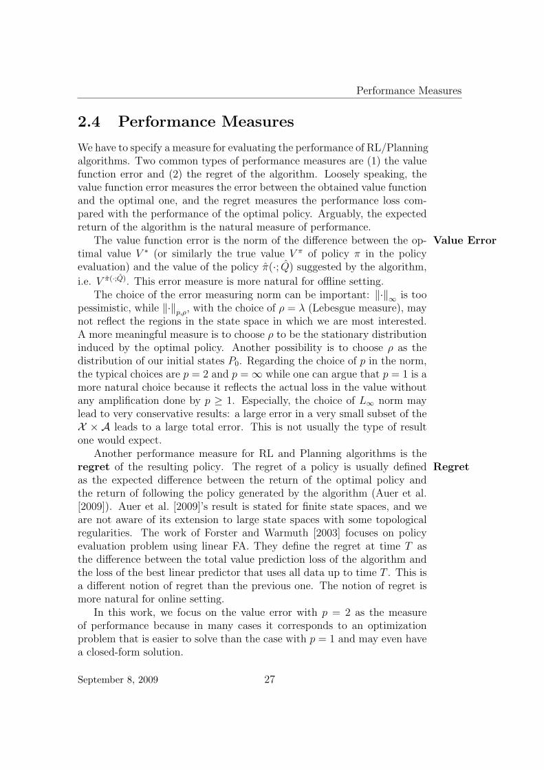
We have to specify a measure for evaluating the performance of RL/Planningalgorithms. Two common types of performance measures are (1) the valuefunction error and (2) the regret of the algorithm. Loosely speaking, thevalue function error measures the error between the obtained value functionand the optimal one, and the regret measures the performance loss com-pared with the performance of the optimal policy. Arguably, the expectedreturn of the algorithm is the natural measure of performance.

The value function error is the norm of the difference between the op- Value Errortimal value V ∗ (or similarly the true value V π of policy π in the policyevaluation) and the value of the policy π(·; Q) suggested by the algorithm,

i.e. V π(·;Q). This error measure is more natural for offline setting.The choice of the error measuring norm can be important: ‖·‖∞ is too

pessimistic, while ‖·‖p,ρ, with the choice of ρ = λ (Lebesgue measure), maynot reflect the regions in the state space in which we are most interested.A more meaningful measure is to choose ρ to be the stationary distributioninduced by the optimal policy. Another possibility is to choose ρ as thedistribution of our initial states P0. Regarding the choice of p in the norm,the typical choices are p = 2 and p =∞ while one can argue that p = 1 is amore natural choice because it reflects the actual loss in the value withoutany amplification done by p ≥ 1. Especially, the choice of L∞ norm maylead to very conservative results: a large error in a very small subset of theX × A leads to a large total error. This is not usually the type of resultone would expect.

Another performance measure for RL and Planning algorithms is theregret of the resulting policy. The regret of a policy is usually defined Regretas the expected difference between the return of the optimal policy andthe return of following the policy generated by the algorithm (Auer et al.[2009]). Auer et al. [2009]’s result is stated for finite state spaces, and weare not aware of its extension to large state spaces with some topologicalregularities. The work of Forster and Warmuth [2003] focuses on policyevaluation problem using linear FA. They define the regret at time T asthe difference between the total value prediction loss of the algorithm andthe loss of the best linear predictor that uses all data up to time T . This isa different notion of regret than the previous one. The notion of regret ismore natural for online setting.

In this work, we focus on the value error with p = 2 as the measureof performance because in many cases it corresponds to an optimizationproblem that is easier to solve than the case with p = 1 and may even havea closed-form solution.



2.5 Reinforcement Learning and Planning

in Large State Spaces

In the value-based approach for solving sequential decision-making prob-lems, we require a way to represent the learned value function. For largestate space X , exact representation of the value for each x ∈ X is imprac-tical or even impossible, and we must use function approximation.

Many researchers have studied the use of FA for RL and planning prob-lems. Without attempting to provide an extensive literature survey ondifferent ways FA has been used in this context, we discuss key aspects ofdifferent methods and provide some exemplar references.

One may categorize the use of function approximation in RL/Planningaccording to (1) the approach to the modeling assumptions (parametric vs.nonparametric), (2) the convergence behavior, and (3) whether the goal ispolicy evaluation or control. In the followings, we discuss these issues indetail.

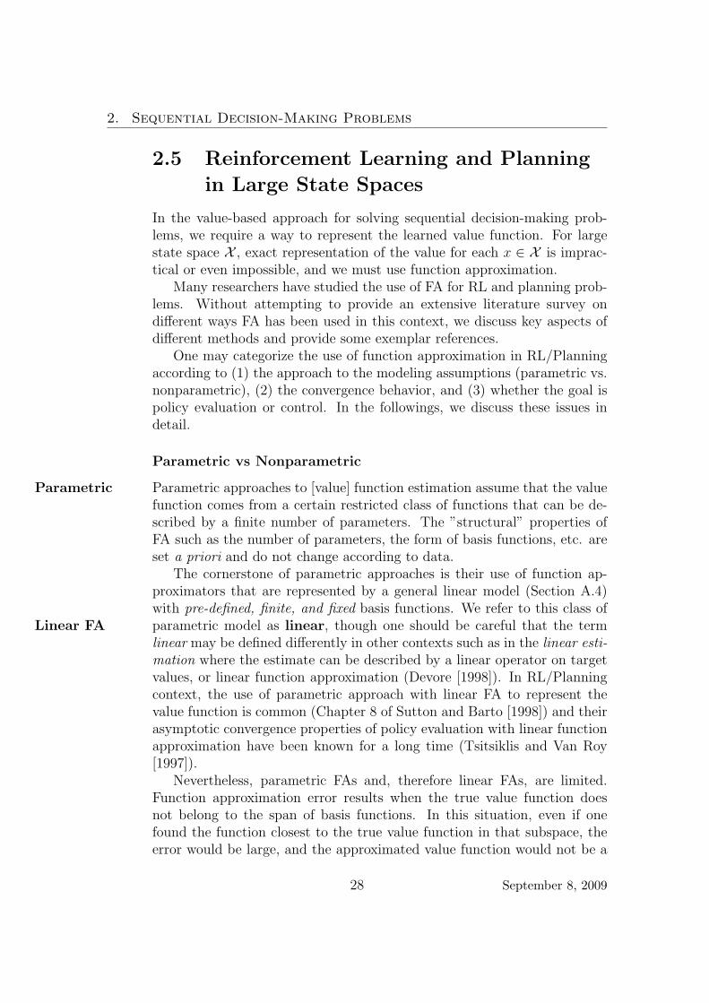
Parametric vs Nonparametric

Parametric approaches to [value] function estimation assume that the valueParametricfunction comes from a certain restricted class of functions that can be de-scribed by a finite number of parameters. The ”structural” properties ofFA such as the number of parameters, the form of basis functions, etc. areset a priori and do not change according to data.

The cornerstone of parametric approaches is their use of function ap-proximators that are represented by a general linear model (Section A.4)with pre-defined, finite, and fixed basis functions. We refer to this class ofparametric model as linear, though one should be careful that the termLinear FAlinear may be defined differently in other contexts such as in the linear esti-mation where the estimate can be described by a linear operator on targetvalues, or linear function approximation (Devore [1998]). In RL/Planningcontext, the use of parametric approach with linear FA to represent thevalue function is common (Chapter 8 of Sutton and Barto [1998]) and theirasymptotic convergence properties of policy evaluation with linear functionapproximation have been known for a long time (Tsitsiklis and Van Roy[1997]).

Nevertheless, parametric FAs and, therefore linear FAs, are limited.Function approximation error results when the true value function doesnot belong to the span of basis functions. In this situation, even if onefound the function closest to the true value function in that subspace, theerror would be large, and the approximated value function would not be a


Reinforcement Learning and Planning in Large State Spaces

good representative of the true one. This leads to poor resulting policies.This issue signifies the importance of the proper choice of basis functions.This choice, however, requires considerable prior knowledge about the valuefunction itself. Moreover, in order to have an adaptive method, the choiceshould depend on some properties of the underlying problem and data,such as the number of available data samples, the geometry of data in in-put space, smoothness of the target function, etc. For instance, in a linearFA architecture, it is not good to have a huge number of basis functionswhen we have only a few samples as the estimation error will blow up. Incontrast, when there are huge amount of data available, restricting ourselvesto a span of a few basis function is not data efficient. Or if the underlyingdata distribution is concentrated on a small subset of the input space, it isreasonable to have more basis functions around that region (assuming theerror measure is w.r.t. the same distribution). Section A.3 provides moreinformation regarding adaptive methods.

Nonparametric approaches, however, have much weaker assumptions on Nonparametricthe statistical model of the [value] function. They do not assume that themodel can best be described by a finite number of parameters and they areflexible in changing their structural properties data-dependently. They im-plicitly or explicitly work with infinite dimensional function spaces. More-over, the choice of basis functions themselves may be adaptive and dependon data. Examples of nonparametric methods are K-NN, smoothing kernelmethods, locally linear models, regularization-based methods in an RKHS(splines), decision trees, neural networks, and orthogonal series estimates(Section A.4).

There have been some attempts in the RL/Planning community to ben-efit from some aspects of nonparametric approaches. One common wayis to use automatic basis adaptation and generation technique. The basisadaptation approaches, which are not usually formulated in a truly non- Basis Adapta-

tionparametric framework, work by parameterizing basis functions (e.g. thecenters of Radial Basis Functions (RBF)) and changing them to optimizean objective function such as an estimate of the Bellman residual error. Forexample, Menache et al. [2005] use both a gradient-based method and thecross-entropy algorithm to find basis parameters that minimize an estimateof the Bellman residual error ‖V (·; θ)− T πV (·; θ)‖X ′) where X ′ ⊂ X is a fi-nite subset of X , and θ in V (·; θ) describes the parameters of basis functions.Yu and Bertsekas [2009] extend this idea to nonlinear T s. These approachesare not nonparametric in the sense that the function space is finite dimen-sional. However, they work with nonlinear FA which is occasionally usedin nonparametric methods.

Generating new basis function data and problem-dependently, as op- Basis Genera-tion



posed to use a fixed pre-defined basis set, is another related nonparametricapproach. One general approach is to benefit from some intrinsic propertiesof the MDP or the induced Markov chain, such as the transition kernel Pand the reward function R, to build basis functions. One idea is to use theset of eigenfunctions of P π, that is ρi : ρiP

π = λiρi, as basis functions. Arelated approach is to use the union of that set with (P π)kR : k = 1, . . ..This is called the augmented Krylov method. These two approaches havebeen suggested by Petrik [2007], who showed its approximation error prop-erties.

A similar basis generation approach is to use the Bellman residual errorfor defining new basis functions (Parr et al. [2007]). This approach startsfrom a single arbitrary basis function, and then estimates the value functionV . If the estimated value function is not the same as the true value function(due to both estimation and approximation error), V − T πV will be a non-zero function. This Bellman residual error defines the new basis function. Itcan be shown that if we ignore the estimation error, repeating this proceduredecreases an upper bound of the approximation error. Parr et al. [2008] showthat if we start from R as basis function for the Bellman residual error basisfunction generation method (Parr et al. [2007]), the result is the same asthe Krylov basis (P π)kR : k = 1, . . . of Petrik [2007].

One must be cautious in interpreting these results. The theoreticalguarantees on decreasing the upper bound of the approximation error arevalid whenever we can find the eigenfunctions of P π, functions (P π)kR, orthe effect of Bellman operator T π on V . Even if we know the model, thesecomputations may be intractable for large MDPs. Moreover, even if we usesample-based approaches to estimate these quantities, as is suggested byParr et al. [2007] for estimating the Bellman residual error function, it isnot evident that the new estimation problem is any easier than the originalvalue function estimation problem.

Another similar basis generation method is a graph Laplacian-basedapproach. This method generates basis functions in accordance with thetransition flow’s geometry of the MDP. This choice might be helpful whenthe geometry of most probable states has some special properties like ly-ing close to a low-dimensional manifold. In this method, basis functionsare eigenfunctions of the graph Laplacian operator. The graph Laplacianoperator is built based on the state transition data and its spectrum con-tain information about the geometry of the transition flow in the state space(Chung [1997]). This method, as opposed to the augmented Krylov methodof Petrik [2007], does not take into account the structure of the reward func-tion. Some may consider this as an advantage because of the transferabilityof basis functions over problems with the same dynamics but different ob-


Reinforcement Learning and Planning in Large State Spaces

jectives, whereas others may consider it as a disadvantage because not allnecessary information has been used (Mahadevan and Maggioni [2007]).

Gaussian Process Temporal Difference (GPTD) is an example of non-parametric method for representing the value function (Engel et al. [2005]).In GPTD, one puts Gaussian Process prior over value functions. By as-suming the independence of ”residuals”, the difference between the valuefunction V (x) and return G(ξ(x)) =

∑∞t=0 γtRt (with the trajectory ξ(x)

starting from X0 = x), one can obtain a closed-form solution for the pos-terior of the value function based on observed data samples. GPTD, likemany other RKHS-based machine learning algorithms, uses data to gener-ate a dictionary of basis functions. GPTD is an example of nonparametricmethod for policy evaluation and GPSARSA is its modification to handlepolicy improvement. Of course, the GP assumption on residuals and theindependence of them make this method not completely rigorous.

As another set of examples of the application of nonparametric and data-dependent approaches in the context of fitted value iteration, Ormoneit andSen [2002] use smoothing kernel-based regression, Ernst et al. [2005] devisetree-based methods to represent the value function, and Riedmiller [2005]apply neural networks in the inner loop of value iteration algorithm.

Our regularized methods, RFQI (Chapter 3), REG-LSTD and REG-BRM (Chapter 4), are instances of nonparametric methods for sequentialdecision-making problems. If we formulate them in an RKHS, they adap-tively generate basis functions to represent the action-value function. Incontrast to basis adaptation/generation algorithms where the basis genera-tion is separated from the value function estimation, in our methods basisgeneration procedure is interwoven with the value function estimation. Ifwe formulate them in a function space with an over-complete dictionary ora Besov space with wavelet basis, l1 regularization-based methods can hope-fully select a subset of basis functions that is required for value functionestimation.

Convergence Behavior

Convergence behavior of an algorithm shows how the agent performs aftercertain amount of interactions with the environment. The study of conver-gence behavior especially becomes more complicated when we are dealingwith RL/Planning problems with large state spaces. The convergence prop-erty of an algorithm can be stated by proving the asymptotic consistencyof the algorithm or by providing a convergence bound. Some algorithmsmay not eventually converge, but still get close to the neighborhood of the”solution”. They may still perform well, but not optimal.



The asymptotic results are more common in RL/Planning literature.For instance, Tsitsiklis and Van Roy [1997] show that estimated value func-tion by the TD method with linear FA asymptotically converges to a close,though not diminishing, neighborhood of the best approximation of the truevalue function in the span of basis functions. This result is asymptotic anddoes not neither show the finite sample behavior nor convergence rate ofthe algorithm. Moreover, because of the parametric representation of FA,the solution of TD with linear FA does not necessary get close to the truevalue function.

Melo et al. [2008] prove that SARSA algorithm, an incremental onlineon-policy value iteration algorithm, with linear FA converges to the fixedpoint of a modified Bellman optimality operator defined by de Farias andVan Roy [2000].4 Their results, although minimal, are still useful. Theyshow that the algorithm will not behave erratically, which is not uncommonin RL/Planning with FA.

Nevertheless, some results study the convergence error bound of thealgorithm. Antos et al. [2008b] study the finite-sample error upper boundsof modification of the Bellman Residual Minimization algorithm used inthe Policy Iteration algorithm, and Munos and Szepesvari [2008] studythe finite-sample convergence behavior of Value Iteration algorithm. Inthis work, we provide finite-sample error upper bounds and, therefore ourresults are similar to the aforementioned work. The difference between ourwork and theirs is that we focus on providing algorithms that use specificregularities of the problem, while others formulate the problem for a generalfunction space.

Policy Evaluation vs. Control

The final aspect of using FA in RL/Planning problems is whether the al-gorithm is designed for the policy evaluation or the algorithm is for controland improves the policy as well.

Two issues make the control problem more challenging. First, whenthe samples come from the stationary distribution ν induced by a policyπ, the new operator defined by the ν-weighted projection of the Bellmanoperator T π onto the linear function space, is a contraction mapping w.r.t.‖·‖ν . This is not, however, the case for the Bellman optimality operatorT ∗. Even worse, the combination of projection and the Bellman optimalityoperator may not even have a fixed point (see de Farias and Van Roy [2000]).

4Melo et al. [2008] proves the asymptotic convergence of Q-Learning under certainconditions, thought it seems that the paper has a bug: it doesn’t show the existence ofthe corresponding fixed point.


Concentrability of Future-State Distribution in MDPs

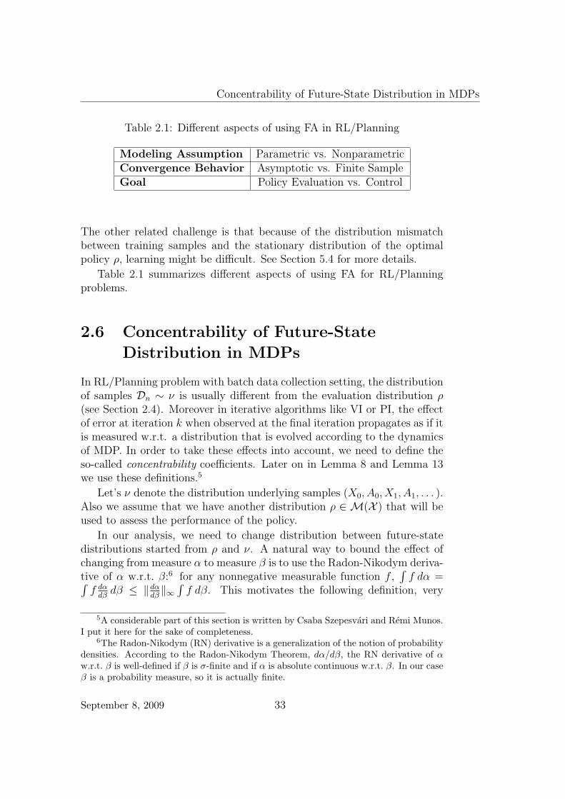
Table 2.1: Different aspects of using FA in RL/Planning

Modeling Assumption Parametric vs. NonparametricConvergence Behavior Asymptotic vs. Finite SampleGoal Policy Evaluation vs. Control

The other related challenge is that because of the distribution mismatchbetween training samples and the stationary distribution of the optimalpolicy ρ, learning might be difficult. See Section 5.4 for more details.

Table 2.1 summarizes different aspects of using FA for RL/Planningproblems.

2.6 Concentrability of Future-State

Distribution in MDPs

In RL/Planning problem with batch data collection setting, the distributionof samples Dn ∼ ν is usually different from the evaluation distribution ρ(see Section 2.4). Moreover in iterative algorithms like VI or PI, the effectof error at iteration k when observed at the final iteration propagates as if itis measured w.r.t. a distribution that is evolved according to the dynamicsof MDP. In order to take these effects into account, we need to define theso-called concentrability coefficients. Later on in Lemma 8 and Lemma 13we use these definitions.5

Let’s ν denote the distribution underlying samples (X0, A0, X1, A1, . . . ).Also we assume that we have another distribution ρ ∈ M(X ) that will beused to assess the performance of the policy.

In our analysis, we need to change distribution between future-statedistributions started from ρ and ν. A natural way to bound the effect ofchanging from measure α to measure β is to use the Radon-Nikodym deriva-tive of α w.r.t. β:6 for any nonnegative measurable function f ,

∫f dα =∫

f dαdβ

dβ ≤ ‖dαdβ‖∞∫

f dβ. This motivates the following definition, very

5A considerable part of this section is written by Csaba Szepesvari and Remi Munos.I put it here for the sake of completeness.

6The Radon-Nikodym (RN) derivative is a generalization of the notion of probabilitydensities. According to the Radon-Nikodym Theorem, dα/dβ, the RN derivative of αw.r.t. β is well-defined if β is σ-finite and if α is absolute continuous w.r.t. β. In our caseβ is a probability measure, so it is actually finite.



similar to the one introduced by Munos and Szepesvari [2008]:

Definition 7 (Discounted-average Concentrability of Future-State Distri-bution). Given ρ ∈ M(X ), ν ∈ M(X × A), m ≥ 0 and an arbitrarysequence of stationary policies πmm≥1, let ρπ1,...,πm ∈ M(X × A) denotethe future state-action distribution obtained when the first state is obtainedfrom ρ and then we follow policy π1, then policy π2, . . ., then πm−1 at whichstep a random action is selected with πm. Define

cρ,ν(m) = supπ1,...,πm

∥∥∥∥d(ρπ1,...,πm)

dν

∥∥∥∥∞

, (2.7)

with the understanding that cρ,ν(m) =∞ if the future state-action distribu-tion ρπ1,...,πm is not absolutely continuous w.r.t. ν. The first-order k-shifted(k ≥ 0, k ∈ N) discounted-average concentrability of future-state distribu-tions is defined by

C(1,k)ρ,ν = (1− γ)

∞∑m=0

γmcρ,ν(m + k).

Similarly, the second-order k-shifted (k ≥ 0, k ∈ N) discounted-averageconcentrability of future-state distributions is defined by

C(2,k)ρ,ν = (1− γ)2

∑m≥1

mγm−1cρ,ν(m + k).

In general cρ,ν(m) diverges to infinity as m → ∞. However, thanks to

discounting, C(i,j)ρ,ν will still be finite whenever γm converges to zero faster

than cρ,ν(m) converges to ∞. In particular, if the rate of divergence ofcρ,ν(m) is sub-exponential, i.e., if Γ = lim supm→∞ 1/m log cρ,ν(m) ≤ 0 then

C(i,j)ρ,ν will be finite.

In the stochastic process literature, Γ is called the top-Lyapunov expo-nent of the system and the condition Γ ≤ 0 is interpreted as a stabilitycondition. Hence, our condition on the finiteness of the discounted-averageconcentrability coefficient Cρ,ν can also be interpreted as a stability condi-tion.

The concentrability coefficients C(i,j)ρ,ν will enter our bound on the weighted

error of the algorithm. In addition to these weighted-error bounds, we willalso derive a bound on the L∞-error of the algorithm. This bound requiresa stronger assumption. Let µ ∈M(X ) and define

Cµ = supx∈X ,a∈A

dP (·|x, a)

dµ,


Concentrability of Future-State Distribution in MDPs

i.e., the supremum of the density of the transition kernel w.r.t. the state-distribution µ. Again, if the system is ”noisy” then Cµ is finite: in fact, thenoisier the dynamics is (the less control we have), the smaller Cµ is. In ourcase µ will be νX , the distribution underlying the states Xt.


Chapter 3

Regularized Fitted Q-Iteration

3.1 Introduction

In this chapter, we introduce the Regularized (or Penalized) Fitted Q-Iteration (RFQI) algorithm. RFQI is a nonparametric approximate valueiteration (AVI) algorithm (see Section 2.3) that can effectively deal withlarge state spaces by exploiting regularities of the value function such as itssmoothness or sparseness.1

Even though AVI can be formulated nonparametrically in different ways,we focus on regularization-based approaches. Nevertheless, the regularization-based approaches themselves may be formulated in various ways. Here, wespecifically focus on developing a Reproducing Kernel Hilbert Space(RKHS)-based formulation for RFQI because of its generality, flexibility,and the ease of incorporating prior knowledge. RKHSs are general becauseone can define them on different spaces ranging from Euclidean spaces tospace of strings and graphs; they are flexible because new function spacescan be defined easily by combining a set of available kernels or changing theparameters of the kernel; and they can easily incorporate prior knowledgeby the choice of the kernel or the change in its parameters. In RKHS-basedformulation, L2-regularized (penalized) least squares regression method isused as the core FA2.

In an RKHS, smoothness is measured by the norm of the space. DifferentRKHSs have different smoothness properties, so if for any a priori reason

1The results of this chapter has been partially published by Farahmand et al. [2008],Farahmand et al. [2009a], and Farahmand et al. [2009d]

2Our use of L2 notation should not be confusing. When we use L2, we are referringto the inner product norm in a specific Hilbert space which should be clear from thecontext, e.g. RKHS norm of the space H. It should not be confused with L2(X ) whichis the set of measurable functions whose its squared-value has finite Lebesgue integral.

37

3. Regularized Fitted Q-Iteration

we believe that some specific type of smoothness measure is more naturalfor the given problem, we can enforce that type of smoothness by our choiceof kernel function and the corresponding RKHS. This makes the suggestedRKHS-based RFQI a flexible method.

RFQI uses regularized (penalized) least squares regression, a nonpara-metric regression method, to estimate T ∗Q for a given Q function basedon samples in the form of T ∗Q(Xt, At)nt=1. If the estimate Qk+1, which isbased on T ∗Qk(Xt, At)nt=1, is close enough to T ∗Qk for all k = 1, 2, . . . , K,and certain concentrability coefficients are finite (Section 2.6), performingAVI procedure will result in a value function QK whose the value of thegreedy policy π(·; QK) is close to the optimal value V ∗.

In Section 3.2, we formulate the problem and provide its algorithmicimplementation. We provide a closed-form solution for an RKHS-basedformulation of RFQI.

To analyze the statistical properties of RFQI, we require two types ofresults. The first is the analysis of the error occurring at each iterationof the AVI, i.e. ‖Qk+1 − T ∗Qk‖ for k = 1, . . . , K. We analyze this errorfor an RKHS-based RFQI in Section 3.4 and provide an almost optimalfinite-sample error upper bound. The second result shows the relation be-tween error at each iteration of AVI and the resulting error after K itera-tions of AVI. Section 3.3 provides a theorem that relates the error between‖Qk+1 − T ∗Qk‖ for k = 1, . . . , K to the error between the optimal valuefunction V ∗ and the value of the resulted policy (V πK ; πK = π(·; QK)), i.e.‖V ∗ − V πK‖. Using these two results, Theorem 10 relates the performanceof the final policy to the performance of the optimal policy given that thealgorithm has a finite amount of data samples. Likewise, we give a perfor-mance bound for the case that we have a limited amount of computationalresources for obtaining the resulting policy.

Knowing how many samples are necessary to achieve a certain per-formance error, even a rough estimate, is important in practice becauseobtaining new samples is expensive in many applications. Examples arewhen we are directly learning from real-world experiences, sampling rateis physically constrained, or we are using a complex and computationallydemanding simulator such as a fluid dynamics simulator or a complex net-work simulator that requires discrete event simulations (see Meyn [2008]).In some other situations, samples are not expensive but computation poweris limited and therefore budgeted. Results of Section 3.4 show that RFQIhas a close to optimal performance even in finite-sample regime.

Later on in this chapter, we briefly mention l1-penalization as a sparsity-enforcing regularization to be used instead of RKHS formulation of RFQIprocedure (Section 3.5). This type of regularization seems to be more nat-


Algorithm

ural when we are working with over-complete dictionaries like wavelets.Section 3.6 suggests some ideas for model selection in RFQI context.

Finally, we discuss several related works in Section 3.7 and compare themwith RFQI.

3.2 Algorithm

RFQI is an approximate value iteration method that iteratively approxi-mates the optimal action-value function Q∗. RFQI belongs to the family ofFitted Q-Iteration algorithms. In this section, we first describe the genericFitted Q-Iteration algorithm and then specialize it to RFQI.

The Fitted Q-Iteration algorithm receives a data set Dn, the number ofAVI iterations K, and Q0 as the initial action-value function. The data sethas the form of

Dn =((X1, A1, R1, X

′1), (X2, A2, R2, X

′2), . . . , (Xn, An, Rn, X

′n)).

where (Xt, At) ∼ ν, and we denote the state-marginal of ν by νX . For thesake of simplifying the analysis, we assume that the actions and next statesare generated by some fixed stochastic stationary policy πb: At ∼ πb(·|Xt),X ′

t ∼ P (·|Xt, At), Rt ∼ R(·|Xt, At).In the planning scenario, νX can be the sampling distribution resulted

from an i.i.d. process that selects states Xt ∼ νX . For RL scenario, samplesusually come from a single trajectory and have the form

(X1, A1, R1, X2, A2, R2, . . . , Xn, An, Rn, Xn+1),

which results in

Dn =((X1, A1, R1, X2), (X2, A2, R2, X3), . . . , (Xn, An, Rn, Xn+1)

).

The Fitted Q-Iteration algorithm, which its pseudo-code is shown inTable 3.1, starts from an initial action-value function Q0. It then usesFitQ(Qk, D, k) procedure to approximately perform a step of value iteration(T ∗Qk) for each iteration k = 0, . . . , K − 1. The FitQ applies the empiricalBellman optimality operator T ∗ (Definition (5)) to data set Dn with Qk asthe current estimate of the optimal action-value function. The FitQ solvesthe regression problem with data set defined by(

(Xt, At), (T∗Qk)(Xt)[= Rt + γ max

a′Q(Xt+1, a

′)])n

t=1,

and returns Qk+1 as the result. This iterative procedure continues K times.3

3Fitted Q-Iteration, like any other value iteration algorithm, can be used both forfinding the optimal policy or evaluating a given policy. We formulate the algorithm forthe former case, but modification of the algorithm for policy evaluation is straightforward.



Fitted Q-Iteration(Dn,K,Q0)// Dn: samples// K: number of iterations// Q0: Initial action-value functionfor k = 0 to K − 1 do

Qk+1 ← FitQ(Qk,Dn, k)end forreturn QK and π(·; QK)

Table 3.1: Fitted Q-Iteration

Regularized Fitted Q-Iteration

In Regularized Fitted Q-Iteration, the regression algorithm in the fittingprocedure, FitQ(Qk, D, k), is Regularized Least-Squares regression. Regu-larized least-squares regression is a nonparametric algorithm that if appliedproperly, can adapt to the problem.

Assuming that in the kth iteration we use mk samples with index nk ≤i < nk + mk = nk+1 − 1, the (k + 1)th iterate is obtained by

Qk+1 = argminQ∈FM

1

mk

nk+mk−1∑i=nk

[Ri + γ max

a′∈AQk(X

′i, a

′)−Q(Xi, Ai)]2

+ λJ(Q),

(3.1)

where J(Q) is the regularizer term and λ > 0 is the regularization coef-ficient.4 The first term is the sample-based least-squares error of using Qto predict R(Xt, At) + γ maxa′∈A Qk(X

′t, a

′) at (Xt, At). This term is theempirical counterpart to the loss

Lk(Q) = E

[(Q(X,A)−

(R(X, A) + γ max

a′∈AQk(X

′, a′)

))2]

.

Fitting a Q function that minimizes this L2 loss is a regression prob-lem where the inputs are (Xi, Ai) ∈ X × A and outputs are R(Xi, Ai) +γ maxa′∈A Qk(X

′i, a

′). Therefore, the minimizer of this L2 loss function isthe regression function

E[R(x, a) + γ max

a′∈AQk(X

′, a′) |X = x, A = a

]= (T ∗Qk)(x, a).

4Here we consider that the data set Dn is chopped into smaller data sets with sizemk each with

∑Kk=1 mk = n. In practice, it is also possible to reuse all samples at each

iteration. In such a case, the analysis must be changed slightly.


Algorithm

Nevertheless when there are only a finite number of samples available,which is always the case in practice, there will be some error between theestimate Qk+1 and the regression function T ∗Qk. The performance of AVIdepends on the size of this error.

Regularized least-squares regression provides an adaptive way to effi-ciently estimate the regression function T ∗Qk and make ‖Qk+1 − T ∗Qk‖as small as possible. In this approach, by the right choice of the regu-larizer J(Q) and the regularization coefficient λ, we can control the com-plexity (or size) of the function space, and therefore avoid overfitting orover-smoothing.

The choice of J(Q) should depend on our belief about the right measureof complexity for FM . Usually one chooses a very large function space FM ,such as the space of all continuous functions, and then effectively confinesthe search for the target function to the subset FM

λ ⊂ FM by changing theregularization coefficient λ. The way J(·) is defined implicitly determinesthe way we prefer to search in that space.

One common choice for regularizer is L2 norm of functions in FM . Thistype of regularization favors smoother solutions to rougher ones (see Sec-tion A.4). The precise definition of smoothness depends on the topologyof FM and the corresponding J(·) and is not necessarily in agreement withthe traditional derivative-based smoothness. For more details, refer to the”Chapter 1: How to Measure Smoothness” of the book by Triebel [2006].

As a side note, regularization has a Bayesian interpretation too. Forinstance, L2 regularization is equivalent to having a Gaussian prior over thespace of functions, and l1 regularization is equivalent to having a Laplacianprior over parameters, see [Rasmussen and Williams, 2006, Section 6.2].Nevertheless, we do not follow Bayesian approach to derive our results,mainly because proving consistency/convergence bounds for the posteriorscan be problematic.

When FM is a Sobolev space5 and J(·) is the corresponding Sobolev-space norm (the squared norm of the generalized partials of Q), the opti-mization problem defined in Eq.(3.1) leads to smoothing spline estimates,popular in the nonparametric statistics literature [Gyorfi et al., 2002].

Sobolev space is a particular case of an RKHS. Thus, more generally,we may start with a Mercer kernel function k, which uniquely defines anRKHS H [Scholkopf and Smola, 2002], and set the norm of Q in that space,‖Q‖H, as the regularizer, i.e. J(Q) = ‖Q‖2H. The RKHS formulation of the

5Sobolev spaces generalize Holder spaces by allowing functions which are only almosteverywhere differentiable. Thus, they can be useful for control problems where value-functions often have ridges. For more details, refer to Appendix B.



optimization problem defined in Eq. (3.1) is

Qk+1 = argminQ∈FM (=H)

1

mk

nk+mk−1∑i=nk

[Ri + γ max

a′∈AQk(X

′i, a

′)−Q(Xi, Ai)]2

+ λ ‖Q‖2H .

(3.2)

According to the Representer Theorem (e.g. Wahba [1990]; Scholkopf et al.[2001]; Scholkopf and Smola [2002]), every solution to Eq. (3.2) is the sumof kernels centered on the observed samples:

Qk+1(x, a) =

nk+mk−1∑i=nk

α(k+1)i−nk+1 k

((Xi, Ai), (x, a)

),

where α(k+1) = (α1, . . . , αmk)> are the coefficient that must be determined.

Let us assume that Qk was obtained previously in a similar form:

Qk(x, a) =

nk−1+mk−1∑i=nk−1

α(k)i−nk−1+1 k

((Xi, Ai), (x, a)

),

and let us collect the coefficients into a vector α(k) ∈ Rmk−1 . Replacing Qin Eq. (3.2) by its expansion and using the fact that ‖Q‖2H = αT Kα inthe RKHS with the K as the Grammian, which will be specified shortly,we would get

α(k+1) = argminα∈Rmk

1

mk

∥∥r + γK+α(k) −Kα∥∥2

+ λα>Kα, (3.3)

with K ∈ Rmk×mk , K+ ∈ Rmk×mk−1 ,

[K]ij = k((Xi−1+nk

, Ai−1+nk), (Xj−1+nk

, Aj−1+nk)),

[K+]ij = k((X ′

i−1+nk, A

(k)i−1+nk

), (Xj−1+nk−1, Aj−1+nk−1

)),

where A(k)j = argmaxa∈A Qk(X

′j, a), and r = (Rnk

, . . . , Rnk+mk−1)>. Solving

Eq. (3.3) for α, we obtain α(k+1) = (K+mkλI)−1(r+γK+α(k)). The com-putational complexity of iteration k with a straightforward implementationis O(m3

k) as it involves the inversion of a matrix.This section described how the RFQI algorithm works. In order to

understand its statistical behavior, we must analyze how much error occursin each iteration and how the error is propagated along iterations. Answersto these questions are the subject of the next two sections.


Error Propagation

3.3 Error Propagation

In this section we provide an upper bound for the norm of V ∗ − V πK andrelate it to the error occurring at each iteration of AVI, ‖Qk+1 − T ∗Qk‖.The analysis of error in each iteration is the subject of Section 3.4.

In order to analyze Fitted Q-iteration we introduce

εk = T ∗Qk −Qk+1 (k ≥ 0); and ε−1 = Q∗ −Q0. (3.4)

These relations define the error sequence εkKk=1 (εk : X × A → R) fromthe sequence of the estimated values Qk. εk shows the difference betweenthe estimated action-value function resulted from taking Qk and solvingEq. (3.1) (or Eq. (3.2) for the specific case of RKHS-based regularization)to obtain Qk+1 and the result of applying the Bellman optimality operatorT ∗ to Qk.

Recall that ν denotes the distribution underlying (Xt, At). For thesake of flexibility, we allow the user to choose another distribution, ρ ∈M(X ), to be used in assessing the performance. Section 2.4 and Section 2.6provide more information on the choice of ρ.

We make the following assumption in our results:

Assumption A1 (MDP Regularity) The set of states X is a compactsubspace of the d-dimensional Euclidean space. The expected immediaterewards r(x, a) =

∫rR(dr|x, a) are bounded by Rmax.

The following lemma holds.

Lemma 8 (Lp-bound). Consider a discounted MDP with a finite numberof actions, and assume Assumption A1 holds. Let p ≥ 1. Assume thatQk and εk satisfy Eq. (3.4) and that πk is a policy greedy w.r.t. Qk. FixK > 0. Define E0 = ‖ε−1‖∞ and εK = max0≤k≤K ‖εk‖p,ν. Then there

exist constants C(1,1)ρ,ν and C

(2,1)ρ,ν that only depend on ρ, ν, γ and the MDP

dynamics such that

‖V ∗ − V πK‖p,ρ ≤ 2

[1

1− γ+

γ

(1− γ)2

]γK/pE0 + 2

[(C

(1,1)ρ,ν )1/p

1− γ+

γ (C(2,1)ρ,ν )1/p

(1− γ)2

]εK .

This lemma bounds the loss of using the learned policy as the function of(1) the losses of the solutions of the regression problems solved while runningthe algorithm and (2) concentrability coefficients of the underlying MDP(see Section 2.6). Lemma 8 shows that if the error sequence εk is uniformlysmall and the concentrability coefficients are small, the error between theoptimal value function V ∗ and the value of our estimated policy V πK issmall too.



3.4 Finite-Sample Convergence Analysis

for RFQI

The goal of this section is to analyze the statistical behavior of errors εk.The result of this section relates the error εk to the sample size mk andthe intrinsic difficulty of the problem. Our analysis is particularly for thecase where Qk+1 is obtained by solving the RKHS regularization problemof Eq. (3.2) for an arbitrary H. The result, Theorem 9, is a tight upperbound for the error of the regularized regression in an arbitrary RKHS H.

We have the following assumptions:

Assumption A2

1. X = [0, 1]d.

2. Samples (Xt, At) ∼ ν are generated i.i.d., and X ′t ∼ P (·|Xt, At).

3. ν is strictly positive measure on X ×A. In particular, we must have

πb0def= mina∈A infx∈X πb(a|x) > 0.

4. k ∈ Lip∗(s, C(X ,X )), s > d.6

5. Qk and T ∗ is such that T ∗Qk ∈ H(= Hk).

6. We assume FM ⊂ B(X ×A; Qmax), for Qmax > 0.

We will shortly discuss the assumptions and the possibility to relaxthem. With these assumptions, the following theorem holds.

Theorem 9 (Farahmand et al. [2008, 2009a]). Let Assumption A2 hold.Let Qk+1 be the solution of (3.2) with some λ > 0. Then

‖Qk+1 − T ∗Qk‖2ν ≤ 2λ ‖T ∗Qk‖2H +c1L

4

mkλd/s+

c2 log(1/δ)

mkL4,

with probability at least 1− δ, for some c1, c2 > 0.

The proof of this result is based on the application of Theorem 4 of Zhou[2003] to generalize Theorem 21.1 of Gyorfi et al. [2002] for an arbitraryRKHS with smooth kernel functions.

Note the trade-off in the bound: increasing λ increases the first term, butdecreases the second. The optimal choice strikes a balance between these

6For the definition of the generalized Lipschitz space Lip∗, see Zhou [2003].


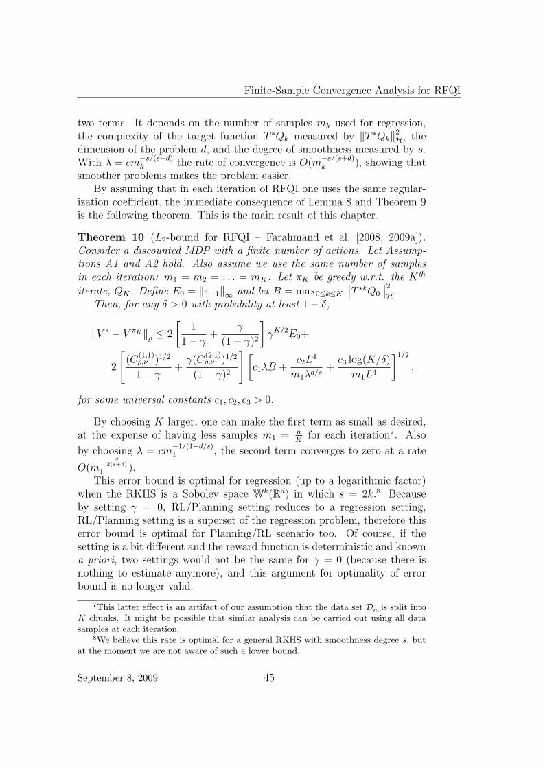
Finite-Sample Convergence Analysis for RFQI

two terms. It depends on the number of samples mk used for regression,the complexity of the target function T ∗Qk measured by ‖T ∗Qk‖2H, thedimension of the problem d, and the degree of smoothness measured by s.With λ = cm

−s/(s+d)k the rate of convergence is O(m

−s/(s+d)k ), showing that

smoother problems makes the problem easier.By assuming that in each iteration of RFQI one uses the same regular-

ization coefficient, the immediate consequence of Lemma 8 and Theorem 9is the following theorem. This is the main result of this chapter.

Theorem 10 (L2-bound for RFQI – Farahmand et al. [2008, 2009a]).Consider a discounted MDP with a finite number of actions. Let Assump-tions A1 and A2 hold. Also assume we use the same number of samplesin each iteration: m1 = m2 = . . . = mK. Let πK be greedy w.r.t. the K th

iterate, QK. Define E0 = ‖ε−1‖∞ and let B = max0≤k≤K

∥∥T ∗kQ0

∥∥2

H.Then, for any δ > 0 with probability at least 1− δ,

‖V ∗ − V πK‖ρ ≤ 2

[1

1− γ+

γ

(1− γ)2

]γK/2E0+

2

[(C

(1,1)ρ,ν )1/2

1− γ+

γ(C(2,1)ρ,ν )1/2

(1− γ)2

] [c1λB +

c2L4

m1λd/s+

c3 log(K/δ)

m1L4

]1/2

,

for some universal constants c1, c2, c3 > 0.

By choosing K larger, one can make the first term as small as desired,at the expense of having less samples m1 = n

Kfor each iteration7. Also

by choosing λ = cm−1/(1+d/s)1 , the second term converges to zero at a rate

O(m− s

2(s+d)

1 ).This error bound is optimal for regression (up to a logarithmic factor)

when the RKHS is a Sobolev space Wk(Rd) in which s = 2k.8 Becauseby setting γ = 0, RL/Planning setting reduces to a regression setting,RL/Planning setting is a superset of the regression problem, therefore thiserror bound is optimal for Planning/RL scenario too. Of course, if thesetting is a bit different and the reward function is deterministic and knowna priori, two settings would not be the same for γ = 0 (because there isnothing to estimate anymore), and this argument for optimality of errorbound is no longer valid.

7This latter effect is an artifact of our assumption that the data set Dn is split intoK chunks. It might be possible that similar analysis can be carried out using all datasamples at each iteration.

8We believe this rate is optimal for a general RKHS with smoothness degree s, butat the moment we are not aware of such a lower bound.



With a simple computational implementation, the cost of executing theprocedure is O(Km3

1). Then given a computational budget B, one mayoptimize K and m1 to get the best possible performance. Clearly, it sufficesto choose K = log(B), hence given the budget B the performance will beO(B−1/(6(1+d/s))).

Remarks on Assumptions

Theorem 9 holds when Assumption A2 is satisfied, and consequently Theo-rem 10 requires the same set of assumptions in addition to Assumption A1,which is needed for the proof of Lemma 8.

In this section, we discuss the significance of conditions in Assump-tion A2 and when one may expect to relax them.

Condition (1) requires that the state space is d-dimensional unit cube.The result is essentially, with the exception of constants, the same for othercompact subsets of Rd with certain boundary regularities. Generalizing ourtheorems to state spaces X other than Rd should be possible under certainconditions such as compactness of the space, though we do not investigateit. See discussions on Condition (4) too.

By Condition (2) samples are to be independent and identically dis-tributed. This assumption basically means that we have access to thegenerative model of the MDP, and is the case for the planning scenario.Nevertheless, this assumption is not essential, and we only use it to sim-plify the proof. We may extend this result to the learning scenario that theagent observes a single trajectory generated by a fixed policy when there isan appropriate mixing condition on the MDP similar to what has been doneby Antos et al. [2008a]. This can be done by independent block technique(Yu [1994]; Doukhan [1994]).

Condition (3) requires that ν should be strictly positive measure on

X × A. In particular, we must have πb0def= mina∈A infx∈X πb(a|x) > 0.

Intuitively, the strict positiveness of ν ensures that we have enough datafrom all over the space of interest. Without that, the value function wouldbe ambiguous in the region where X0 × A0|ν(X0 × A0) = 0; X0 × A0 ⊂X ×A.

Nevertheless, it is possible that with the help of some extra prior knowl-edge about Q(·), we reliably infer the value function on regions from wherethere is no sample. For example, consider a problem with X = [0, 10π]. Ifby some prior knowledge we know that the value function Q(x, a) is peri-odic in states with the period of π, we can infer its value on X even thoughsamples are coming from [0, π] ⊂ X . This type of prior knowledge may beencoded in the kernel function k, but we will not investigate this issue.


Sparsity Regularities and l1 Regularization

The Condition (4) is used to embed the RKHS with k into Cs2 (X )

(Proposition 3 of Zhou [2003]). This embedding implies that a ball withfinite radius in H has well-behaved covering number growth (Theorem 4 ofZhou [2003]). In order to generalize our results for state spaces other thanRd, we require a covering number result that shows the covering number ofspace F : X 7→ R has a gentle behavior.

Condition (5) ensures that the effect of the Bellman optimality operatoron a Qk ∈ H belongs to the same spaceH. This is reasonable if the operatorhas some ”smoothing” behavior (as defined by the norm of H). At present,we do not have any general theory relating this assumption to the morebasic properties of MDP, but we will analyze it in the future.

Finally, Condition (6) is about the uniform boundedness of the functionsin the selected function space. If the solutions of our optimization problemsare not bounded, they must be truncated, and thus, truncation argumentsshould be used in the analysis (For example, see the proof of Theorem 20.3or Lemma 10.2 of Gyorfi et al. [2002]). Truncation does not change thefinal result, so we do not address it in order to avoid unnecessary clutter.

3.5 Sparsity Regularities and l1Regularization

Regularization is indeed not limited to RKHS. Apart from finite dimen-sional spaces, which lead to a formulation similar to the ridge regression, apromising class of candidate function spaces is the class of functions definedby wavelet basis or other function spaces with over-complete dictionaries.Wavelets and over-complete dictionaries are intriguing because upon appro-priate design choices they can capture spatial irregularities like spikes andother spatial heterogeneity, that may occur in the action-value function.

Our approach to deal with wavelets or over-complete dictionaries is us-ing l1 regularized regression, which can be formulated as LASSO problem(Eq. (A.6) in Section A.4). The change to our current formulation is re-placing the regularizer from an RKHS norm of the action-value functionto J(Q(·, ·; θ)) = |θ|T1 in Eq. (3.1) where θ is the coefficient of the lin-ear expansion of the action-value function in the selected function space,and 1 is the vector of all 1s. More specifically, assume Q(·, ·; θ) ∈ Fp =Φ(·, ·)T θ|θ ∈ Rp, Φ(·) : Rd 7→ Rp where Φ(·, ·) are defined by waveletexpansion or over-complete bases. Then the optimization will be



Qk+1(·, ·; θk+1) =

argminQ∈FM (=Fp)

1

mk

nk+mk−1∑i=nk

[Ri + γ max

a′∈AΦ(X ′

i, a′)T θk − Φ(Xi, Ai)

T θ]2

+ λ|θ|T1.

Proving error bound for this l1 penalization-based RFQI is the subjectof further research.

3.6 Model Selection for Regularized Fitted

Q-Iteration

Lemma 8 suggests that to have a close to optimal solution, εK should besmall. Smallness of εK implies that all εk should have small norms, which ac-cording to Theorem 9, means that we must choose λ appropriately. Choos-ing λ = cm

−1/(1+d/s)k gives the exponent-wise optimal rate of convergence.

As we discuss shortly, this choice, however, is not satisfactory.First of all, following a predetermined schedule for the regularization co-

efficient does not imply that the convergence error bound is optimal becauseof the unknown constants in the optimal schedule such as ‖T ∗Qk‖2H.

Furthermore, the smoothness degree of the target function is not usuallyknown a priori. This means that one may violate the T ∗Qk ∈ H(= Hk)assumption. Violation of this assumption leads to an approximation error,i.e. the error between the best possible function in the function class Hk

and the true target function T ∗Qk, i.e. infQ∈Hk‖Q− T ∗Qk‖ν .

These concerns suggest that we need to do data-dependent model se-lection among several available hypothesis classes. Computational issuesaside, one should do model selection at each iteration of RFQI. This isimportant because the appropriate regularization coefficients and even thefunction spaces, which is determined by the kernel parameter, may changeduring iterations.

We discuss model selection problem for RL/Planning in more detail inChapter 5. For now, assume that we want to minimize each ‖εk‖ν .

In this case, the problem of model selection for RFQI is not very dif-ficult, and the approach taken in regression setting can be followed here:Try different smoothness orders, which corresponds to different regularizers,with different regularization coefficients and select the best one by the aidof a hold-out set. This leads to estimate whose convergence bound has theoptimal order and scales with the actual roughness J(TQk).


Related Works

The remaining problem is that because ν and ρ are not necessarily thesame, C1

ρ,ν and C2ρ,ν in our bounds (Lemma 8) might be large numbers. The

suggested model selection method does not consider this effect. We furtherstudy this problem in Section 5.4.

3.7 Related Works

RFQI is similar to the Fitted Q-Iteration algorithm of Ernst et al. [2005]with the difference that the intermediate value functions are obtained bysolving a regularized least-squares regression problem instead of using atree-based approach. Although tree-based methods can be computationallycheap, the conventional implementations of them do not consider regulari-ties like smoothness of the target function.

Along other attempts similar to ours, we can mention Jung and Polani[2006] and Loth et al. [2007]. Nevertheless, these results do not provide anexplicit performance analysis like ours do. Also Jung and Polani [2006] onlyworks for the deterministic transitions with a fixed policy where RFQI isfor control problems with stochastic transitions.

Although finite-sample performance of fitted Q-iteration has been con-sidered earlier [Antos et al., 2008a], to our best knowledge this (and theresults in Chapter 4) are the first work that address finite-sample perfor-mance of a regularized RL/Planning algorithm.

The Fitted Q-Iteration for policy evaluation problems resembles LSPE(Yu and Bertsekas [2007]), which can be considered as another value iteration-based method for RL/Planning. Based on notation used in Yu and Bert-sekas [2007], if we select λ = 0 for the eligibility trace and γ = 1 for theupdate rule (and not the conventional γ used for the discount factor), weretrieve the Fitted Q-Iteration with linear function approximator. Extend-ing the regularization ideas presented in this chapter to LSPE seems to bepossible. The regression part should more or less be the same. The errorpropagation part, however, requires a new analysis as Yu and Bertsekas[2007]’s proofs are asymptotic in nature and are not directly applicable toour desired finite sample-size results.


Chapter 4

Regularized Policy Iteration

4.1 Main Idea

In this chapter, we introduce two regularized-based nonparametric approx-imate policy iteration algorithms (see Section 2.3), namely RegularizedBellman Residual Minimization (REG-BRM) and RegularizedLeast-Squares Temporal Difference (REG-LSTD) algorithms.5-50These methods can effectively deal with large state spaces by exploitingregularities of the value function such as its smoothness or sparseness.1

RKHS-based L2 regularization is used to develop new policy evaluationalgorithms, which are required for policy improvement procedure, basedon the extension of classical methods of BRM and LSTD (Bradtke andBarto [1996]; Lagoudakis and Parr [2003] for LSTD; Williams and Baird[1993]; Antos et al. [2008b] for BRM). We will refer these extensions asREG-BRM and REG-LSTD in the following discussion. We may oc-casionally use REG-LSPI to refer to the combination of REG-LSTD withpolicy improvement procedure, but we will not introduce a new term for thecombination of REG-BRM and policy improvement. The way REG-BRMis used should be clear from the context.

One important difference between the methods introduced in this chap-ter and the Regularized Fitted Q-Iteration (RFQI) of Chapter 3 is thatRFQI is an instance of fixed-point iteration algorithms, whereas REG-LSTDand REG-BRM are direct methods. Another difference is that the goal ofRFQI is finding Q∗ while the goal of REG-LSTD and REG-BRM is findingQπ for a given π. However, one may use RFQI for policy evaluation too,and in this case all methods would have the same goal.

1The results of this chapter has been partially published by Farahmand et al. [2009b].

51

4. Regularized Policy Iteration

The specific problem setting of this chapter is similar to that of Chap-ter 3. We want to find a good policy in an offline data collection settingwith batch processing of data (Section 2.2) for discounted MDPs with largeor even infinite state spaces and finite action spaces.

After reviewing the necessary background on the approximate policyevaluation in Section 4.2, we formulate the policy evaluation problem as anoptimization problem in an infinite-dimensional RKHS, and provide theirclosed-form solution in Section 4.3. We also present finite-sample perfor-mance bounds for the algorithms in Section 4.4. In particular, we show thatthey can achieve a rate that is as good as the corresponding regression ratewhen the value function belongs to a known smoothness class. We furthershow that this convergence behavior carries through to the performanceof a policy found by running policy iteration with our regularized policyevaluation methods. The results indicate that from the point of view oferror upper bounds, RL/Planning is not harder than regression estimation.Section 4.5 discusses the possibility of l1-regularized policy iteration, andexplains the challenge in solving the corresponding optimization problem.Finally, in Section 4.6 we describe other attempts in using regularization-based or similar approaches in the context of policy iteration algorithms.

4.2 Approximate Policy Evaluation

The approximate policy evaluation problem, which is to find a close enoughapproximation V (or Q) of the value function V π (or Qπ) for a given policyπ, is the core requirement for the policy iteration algorithm. In this section,we review two direct policy evaluation algorithms, namely BRM and LSTD,that can be used for MDPs with large state spaces. We formulate them asoptimization problems and provide a geometrical interpretation of them.

The policy evaluation problem is non-trivial for at least two reasons.First, it is an instance of inverse problems2. If we had access to Qπ at anumber of data points in the form of

((Xt, At), Qπ(Xt, At))1≤t≤n,

the policy evaluation problem would be boiled down to the traditional re-gression problem. However, in the context of RL/Planning, we do notusually have access to Qπ(Xt, At) or even an unbiased noisy estimate ofthem3.

2Given an operator L : F 7→ F , the inverse problem is the problem of solving g = Lffor f when g is known.

3An exception is when we use roll-out to provide training samples.


Approximate Policy Evaluation

The second problem is that the observations do not necessarily comefrom following the target policy π, but from a behavior policy πb 6= π. Be-cause of this difference, the distribution of samples is likely to differs fromthe the induced distribution of the target policy. This is often referred toas the off-policy learning problem in the RL literature. This mismatch be-tween the behavior policy and the desired policy is similar to the problemwhen training and test distributions differ in supervised learning setting,and is called distribution mismatch, covariate shift, or sample selec-tion bias problem in the supervised learning community.

In the following subsections, we review generic LSTD and BRM methodsfor policy evaluation. Afterwards, we introduce our regularized version ofLSTD and BRM in Section 4.3. For more details on value iteration-basedalgorithms for policy evaluation, the other alternative, see Chapter 3.

Bellman Residual Minimization

The idea of Bellman residual minimization (BRM) goes back at least tothe work of Schweitzer and Seidmann [1985]. It was later used in the RLcommunity by Williams and Baird [1993] and Baird [1995]. The basic ideaof BRM comes from noticing that the action-value function (or similarly,value function), is the unique fixed point of the Bellman operator: Qπ =T πQπ. Whenever we replace Qπ by another action-value function Q 6= Qπ,the fixed-point equation would not hold anymore, and we have a non-zeroresidual function, i.e. Q − T πQ 6= 0. This quantity is called the Bellmanresidual of Q. The same is true for the optimal Bellman operator T ∗.

Intuitively, if the norm of the optimal Bellman residual, ‖Q− T ∗Q‖, issmall, then Q should be a good approximation of Q∗. This intuition canbe formalized by relating the difference between the optimal value func-tion V ∗ and V π(·;Q) (the value function of the greedy policy w.r.t. Q)that is

∥∥V ∗ − V π(·;Q)∥∥ to the difference between Q and T ∗Q, quantified by

‖Q− T ∗Q‖.Williams and Baird [1993] provide such a formalism when the difference

between Q and T ∗Q is measured by an infinity norm, i.e., ‖Q− T ∗Q‖∞. Inthat case, we have results like

∥∥V ∗ − V π(·;Q)∥∥∞ ≤

2

1− γ‖Q− T ∗Q‖∞ .

Infinity norm, however, is too sensitive in many practical situations.This is especially the case when we are dealing with large state spaces forwhich one must use function approximation. Point-wise convergence results



are not abundant in supervised learning theory, and we doubt if it is a goodidea to go for them in the RL/Planning context either.

To make this point clearer, consider a situation where the agent usesQ as an approximation to the optimal action-value function Qπ, and usesπ(·; Q) as its policy. Moreover, we are measuring the performance of theagent with respect to the evaluation distribution ρ. For example, if ρ is theLebesgue measure on X , it indicates that the performance of the agent inall states are equally important for us. Now consider that Q = Qπ in allstate space except a ρ-small region X1×A1 ⊂ X ×A, i.e., ρ(X1×A1) << 1.In X1×A1, Q is largely different from Q∗(·)|X1×A1 . Here, ‖Q− T ∗Q‖∞ hasa large value, however, the performance of the agent following π(·; Q) isvery close to optimal.

It is more natural to use a weighted Lp-norms such as L2-norm to mea-sure the magnitude of the Bellman residual. First, it leads to a tractableoptimization problem and enables an easy connection to regression functionestimation (Gyorfi et al. [2002]). More importantly, there are certain resultsrelating

∥∥V ∗ − V π(·;Q)∥∥

pand ‖Q− T ∗Q‖p for general p ≥ 1 (Lemma 13 and

Lemma 15). These results show that minimizing Lp norm of the Bellmanresidual actually leads to minimizing the value error performance measure(Section 2.4).

We define the following loss function

LBRM(Q; π) = ‖Q− T πQ‖2ν ,

where ν is the stationary distribution of states in the input data. UsingEq. (2.6) with samples (Xt, At) and by replacing (T πQ)(Xt, At) with theempirical Bellman operator (Definition (5)),

(T πQ)(Xt, At) = Rt + γQ(Xt+1, π(Xt+1)),

the empirical counterpart of LBRM(Q; π) can be written as

LBRM(Q; π, n)def=∥∥∥Q− T πQ

∥∥∥2

n(4.1)

def=

1

nM

n∑t=1

[Q(Xt, At)−

(Rt + γQ

(Xt+1, π(Xt+1)

))]2.

Nevertheless, it is well-known that LBRM is not an unbiased estimateof LBRM for dynamical systems with stochastic transitions (e.g., see Sutton


Approximate Policy Evaluation

and Barto [1998]; Lagoudakis and Parr [2003]; Antos et al. [2008b]):

E[LBRM(Q; π, n)

]= E

[∥∥∥Q− T πQ∥∥∥2

n

]= E

[‖Q− T πQ‖2n +

∥∥∥T πQ− T πQ∥∥∥2

n

]6= LBRM(Q; π). (4.2)

The reason, as is evident in Eq. (4.2), is that stochastic transitions/rewardslead to a non-vanishing variance term because T πQ 6= T πQ. This extraterm can be problematic. Whenever the dynamical system has stochastictransitions, this variance term is not fixed and is Q-dependent. Therefore,minimizing LBRM does not lead to the same solution as minimizer of LBRM

even in the imaginary situation of not having any estimation error. Onthe other hand, if the transition kernel is deterministic but the reward isstochastic, even though the loss would be still biased, ignoring the esti-mation error, the solution of the minimizer of LBRM and LBRM are thesame.

One suggestion to deal with this problem is to use double-sampling toestimate LBRM . According to this proposal, from each state-action pair inthe sample, we require to have at least two independent next-state samples(e.g., see Sutton and Barto [1998]). Nevertheless, this suggestion may notbe practical in many cases. The luxury of having two next-state samplesis not available in RL setting. Even if we have a generative model of theenvironment, as we do in planning scenario, the result would not be sample-efficient, which is important when generating new samples is costly.

Antos et al. [2008b] recently proposed modified BRM that is a newempirical loss function with an extra de-biasing term. The idea of the mod-ified BRM is to cancel the unwanted variance by introducing an auxiliaryfunction h and a new loss function

LBRM(Q, h; π) = LBRM(Q; π)− ‖h− T πQ‖2ν , (4.3)

and approximating the action-value function Qπ by solving

QBRM = argminQ∈FM

suph∈FM

LBRM(Q, h; π), (4.4)

where the supremum comes from the negative sign of ‖h− T πQ‖2ν . Theyhave shown that optimizing the new loss function still makes sense and theempirical version of this loss is unbiased.

Solving Eq. (4.4) is equivalent to solve the following coupled (nested)optimization problems:



h∗Q = argminh∈FM

‖h− T πQ‖2ν ,

QBRM = argminQ∈FM

[‖Q− T πQ‖2ν −

∥∥h∗Q − T πQ∥∥2

ν

]. (4.5)

Of course in practice, T πQ is replaced by its sample-based approximationT πQ.

In this thesis, we only work with the modified BRM and from now on,whenever we refer to the BRM, we mean the modified BRM.

Least-Squares Temporal Difference Learning

Least-Squares Temporal Difference learning (LSTD) was first proposed byBradtke and Barto [1996] for policy evaluation, and later was used for policyimprovement by Lagoudakis and Parr [2003]. Lagoudakis and Parr [2003]call the combination of policy improvement algorithm and LSTD-basedpolicy evaluation, the Least-Squares Policy Iteration (LSPI) algorithm.

The original formulation of LSTD finds a solution to the fixed-pointequation Q = ΠνT

πQ, where Πν is the ν-weighted projection operator ontothe space of admissible function FM , i.e. Π : B(X × A) → B(X × A) isdefined by Πf = argminh∈FM ‖h− g‖2ν for g ∈ B(X × A). If the operatorΠνT

π is a contraction operator, Banach fixed-point theorem (Theorem 28)implies that the combined operator has a unique fixed-point.

Nevertheless, the operator (ΠνTπ) is not contraction for arbitrary choice

of ν unless ν is the stationary distribution induced by π. Therefore, whenthe distribution of samples (X1, At) ∼ ν is different from the stationarydistribution induced by π, this equation does not necessarily have a uniquefixed point.

One can, however, define LSTD solution as the minimizer of the L2

distance between Q and ΠT πQ:

LLSTD(Q; π) = ‖Q− ΠT πQ‖2ν .

Whenever ν is the stationary distribution of π, the solution of this op-timization problem is the same as the fixed-point of Q = ΠνT

πQ.

The LSTD solution can therefore be written as the solution of the fol-lowing coupled optimization problems:


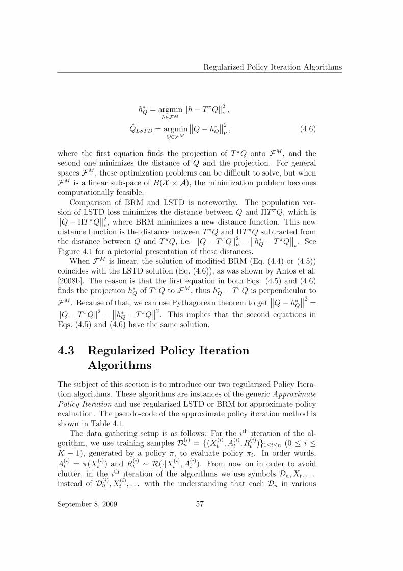
Regularized Policy Iteration Algorithms

h∗Q = argminh∈FM

‖h− T πQ‖2ν ,

QLSTD = argminQ∈FM

∥∥Q− h∗Q∥∥2

ν, (4.6)

where the first equation finds the projection of T πQ onto FM , and thesecond one minimizes the distance of Q and the projection. For generalspaces FM , these optimization problems can be difficult to solve, but whenFM is a linear subspace of B(X × A), the minimization problem becomescomputationally feasible.

Comparison of BRM and LSTD is noteworthy. The population ver-sion of LSTD loss minimizes the distance between Q and ΠT πQ, which is‖Q− ΠT πQ‖2ν , where BRM minimizes a new distance function. This newdistance function is the distance between T πQ and ΠT πQ subtracted fromthe distance between Q and T πQ, i.e. ‖Q− T πQ‖2ν −

∥∥h∗Q − T πQ∥∥

ν. See

Figure 4.1 for a pictorial presentation of these distances.When FM is linear, the solution of modified BRM (Eq. (4.4) or (4.5))

coincides with the LSTD solution (Eq. (4.6)), as was shown by Antos et al.[2008b]. The reason is that the first equation in both Eqs. (4.5) and (4.6)finds the projection h∗Q of T πQ to FM , thus h∗Q − T πQ is perpendicular to

FM . Because of that, we can use Pythagorean theorem to get∥∥Q− h∗Q

∥∥2=

‖Q− T πQ‖2 −∥∥h∗Q − T πQ

∥∥2. This implies that the second equations in

Eqs. (4.5) and (4.6) have the same solution.

4.3 Regularized Policy Iteration

Algorithms

The subject of this section is to introduce our two regularized Policy Itera-tion algorithms. These algorithms are instances of the generic ApproximatePolicy Iteration and use regularized LSTD or BRM for approximate policyevaluation. The pseudo-code of the approximate policy iteration method isshown in Table 4.1.

The data gathering setup is as follows: For the ith iteration of the al-gorithm, we use training samples D(i)

n = (X(i)t , A

(i)t , R

(i)t )1≤t≤n (0 ≤ i ≤

K − 1), generated by a policy π, to evaluate policy πi. In order words,

A(i)t = π(X

(i)t ) and R

(i)t ∼ R(·|X(i)

t , A(i)t ). From now on in order to avoid

clutter, in the ith iteration of the algorithms we use symbols Dn, Xt, . . .instead of D(i)

n , X(i)t , . . . with the understanding that each Dn in various



FM Q

T!Q

!T!Q

minimized by BRM

minimized by LSTD

Figure 4.1: This figure shows the loss functions minimized by BRM, mod-ified BRM, and LSTD methods. The function space FM is representedby the plane. The Bellman operator, T π, maps an action-value functionQ ∈ FM to a function T πQ. The difference between T πQ and its projec-tion to FM , ΠT πQ, is orthogonal to the function space FM . The originalBRM loss function is the squared Bellman error, the distance of Q and T πQ.In order to obtain the modified BRM loss, the squared distance betweenT πQ and ΠT πQ is subtracted from the squared Bellman error. LSTD aimsat a function Q that has minimum distance to ΠT πQ. LSTD and BRM areequivalent for linear function spaces.

iterations is referring to a different set of data samples. The exact referenceshould be clear from the context.

There are various possibilities for choosing the data-generating policyπ. The first is selecting a pre-defined stochastic stationary policy πb. Theother is using a policy based on the most recent estimate of the action-value function, i.e. Q(i−1). This can be the greedy policy w.r.t. Q(i−1)

with some exploration, i.e. π(·; Q(i−1))⊕∆π, where ∆π is a perturbation tothe greedy policy4. If we want to choose policy based on the most recentaction-value function, we require to define Q(−1) to initialize the first policy.

4∆π : X × A 7→ [0, 1] is a function of state and action with the property that∑Mi=1 ∆π(x, ai) ≤ 1 for all x ∈ X . The perturbed policy π(·;Q)⊕∆π defines a probability

distribution of action selection at each state as

π(x;Q)⊕∆πdef=

π(x;Q) with probability 1−

∑Mi=1 ∆π(x, ai)

ai with probability ∆π(x, ai)

This policy is not deterministic.


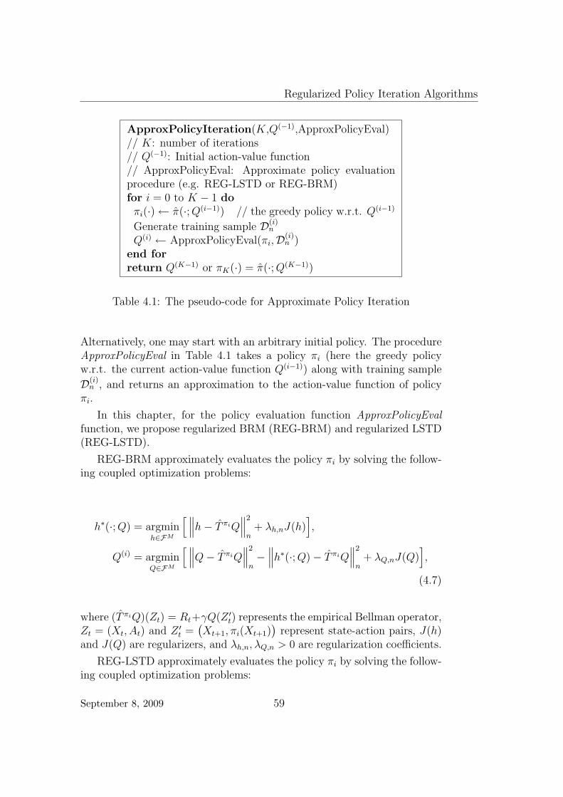
Regularized Policy Iteration Algorithms

ApproxPolicyIteration(K,Q(−1),ApproxPolicyEval)// K: number of iterations// Q(−1): Initial action-value function// ApproxPolicyEval: Approximate policy evaluationprocedure (e.g. REG-LSTD or REG-BRM)for i = 0 to K − 1 doπi(·)← π(·; Q(i−1)) // the greedy policy w.r.t. Q(i−1)

Generate training sample D(i)n

Q(i) ← ApproxPolicyEval(πi,D(i)n )

end forreturn Q(K−1) or πK(·) = π(·; Q(K−1))

Table 4.1: The pseudo-code for Approximate Policy Iteration

Alternatively, one may start with an arbitrary initial policy. The procedureApproxPolicyEval in Table 4.1 takes a policy πi (here the greedy policyw.r.t. the current action-value function Q(i−1)) along with training sample

D(i)n , and returns an approximation to the action-value function of policy

πi.

In this chapter, for the policy evaluation function ApproxPolicyEvalfunction, we propose regularized BRM (REG-BRM) and regularized LSTD(REG-LSTD).

REG-BRM approximately evaluates the policy πi by solving the follow-ing coupled optimization problems:

h∗(·; Q) = argminh∈FM

[ ∥∥∥h− T πiQ∥∥∥2

n+ λh,nJ(h)

],

Q(i) = argminQ∈FM

[ ∥∥∥Q− T πiQ∥∥∥2

n−∥∥∥h∗(·; Q)− T πiQ

∥∥∥2

n+ λQ,nJ(Q)

],

(4.7)

where (T πiQ)(Zt) = Rt+γQ(Z ′t) represents the empirical Bellman operator,

Zt = (Xt, At) and Z ′t =

(Xt+1, πi(Xt+1)

)represent state-action pairs, J(h)

and J(Q) are regularizers, and λh,n, λQ,n > 0 are regularization coefficients.

REG-LSTD approximately evaluates the policy πi by solving the follow-ing coupled optimization problems:



h∗(·; Q) = argminh∈FM

[ ∥∥∥h− T πiQ∥∥∥2

n+ λh,nJ(h)

],

Q(i) = argminQ∈FM

[‖Q− h∗(·; Q)‖2n + λQ,nJ(Q)

]. (4.8)

It is important to note that unlike the non-regularized case described inSections 4.2, REG-BRM and REG-LSTD do not have the same solution.This is because, although the first equations in Eqs. (4.7) and (4.8) arethe same, the function h∗(·; Q) − T πiQ is not necessarily perpendicular tothe admissible function space FM . This is due to the regularization termλh,nJ(h). As a result, the Pythagorean theorem is not applicable anymore:

‖Q− h∗(·; Q)‖2 6=∥∥∥Q− T πiQ

∥∥∥2

−∥∥∥h∗(·; Q)− T πiQ

∥∥∥2

,

therefore the objective functions of the second equations in Eqs. (4.7) and(4.8) are not equal and they do not share the same solution.

Closed-Form Solutions

Depending on how we define FM and the corresponding penalty term J(·),these optimization problems can be easy or difficult to solve. For example,if FM is a finite dimensional linear space, and J(·) is defined as the squaredsum of parameters describing the function, a setup similar to the ridgeregression (Section A.4), the coupled optimization problems have closed-form solutions. Nevertheless, finite dimensional parametric spaces with aset of pre-defined basis functions is not our main interest. We would liketo work with much richer spaces, even infinite dimensional spaces, that canapproximate a large class of functions arbitrary well (see Section 2.5 andSection A.4 for more discussion).

A flexible and powerful possibility for choosing the function space FM

is to work with reproducing kernel Hilbert spaces defined by a positivedefinite kernel K, and the corresponding RKHS norm ‖·‖2H as the penaltyterm J(·). Working with the RKHS not only gives us the flexibility tochoose the function space, but also let us have a closed-form solution to theregularized optimization problems defined by Eqs. (4.7) and (4.8).

The main trick is to use an extension of the Representer theorem for thecoupled optimization problems (Scholkopf et al. [2001]). This Representertheorem states that the infinite dimensional optimization problem defined


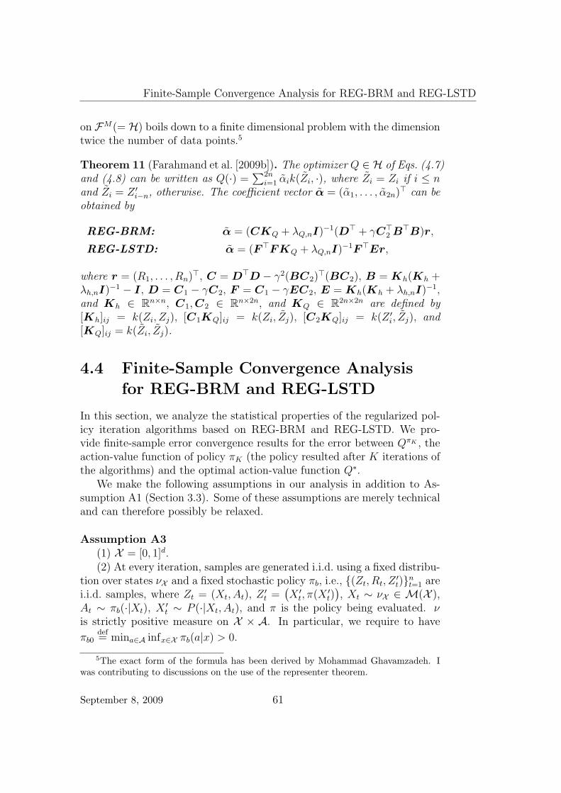
Finite-Sample Convergence Analysis for REG-BRM and REG-LSTD

on FM(= H) boils down to a finite dimensional problem with the dimensiontwice the number of data points.5

Theorem 11 (Farahmand et al. [2009b]). The optimizer Q ∈ H of Eqs. (4.7)and (4.8) can be written as Q(·) =

∑2ni=1 αik(Zi, ·), where Zi = Zi if i ≤ n

and Zi = Z ′i−n, otherwise. The coefficient vector α = (α1, . . . , α2n)> can be

obtained by

REG-BRM: α = (CKQ + λQ,nI)−1(D> + γC>2 B>B)r,

REG-LSTD: α = (F>FKQ + λQ,nI)−1F>Er,

where r = (R1, . . . , Rn)>, C = D>D − γ2(BC2)>(BC2), B = Kh(Kh +

λh,nI)−1 − I, D = C1 − γC2, F = C1 − γEC2, E = Kh(Kh + λh,nI)−1,and Kh ∈ Rn×n, C1, C2 ∈ Rn×2n, and KQ ∈ R2n×2n are defined by[Kh]ij = k(Zi, Zj), [C1KQ]ij = k(Zi, Zj), [C2KQ]ij = k(Z ′

i, Zj), and[KQ]ij = k(Zi, Zj).

4.4 Finite-Sample Convergence Analysis

for REG-BRM and REG-LSTD

In this section, we analyze the statistical properties of the regularized pol-icy iteration algorithms based on REG-BRM and REG-LSTD. We pro-vide finite-sample error convergence results for the error between QπK , theaction-value function of policy πK (the policy resulted after K iterations ofthe algorithms) and the optimal action-value function Q∗.

We make the following assumptions in our analysis in addition to As-sumption A1 (Section 3.3). Some of these assumptions are merely technicaland can therefore possibly be relaxed.

Assumption A3(1) X = [0, 1]d.(2) At every iteration, samples are generated i.i.d. using a fixed distribu-

tion over states νX and a fixed stochastic policy πb, i.e., (Zt, Rt, Z′t)nt=1 are

i.i.d. samples, where Zt = (Xt, At), Z ′t =

(X ′

t, π(X ′t)), Xt ∼ νX ∈ M(X ),

At ∼ πb(·|Xt), X ′t ∼ P (·|Xt, At), and π is the policy being evaluated. ν

is strictly positive measure on X × A. In particular, we require to have

πb0def= mina∈A infx∈X πb(a|x) > 0.

5The exact form of the formula has been derived by Mohammad Ghavamzadeh. Iwas contributing to discussions on the use of the representer theorem.



(3) The function space F used in the optimization problems in Eqs. (4.7)and (4.8) is a Sobolev space Wk(Rd) with 2k > d. Jk(Q) denotes the normof Q in Wk(Rd).

(4) The function space FM contains the true action-value function, i.e.,Qπ ∈ FM .

(5) For every function Q ∈ FM with bounded norm Jk(Q), its im-age under the Bellman operator, T πQ, is in the same space, and we haveJk(T

πQ) ≤ BJk(Q), for some positive and finite B, which is independentof Q.

(6) We assume FM ⊂ B(X ×A; Qmax), for Qmax > 0.

Remarks on Assumptions

By Condition (1), the state space is d-dimensional unit cube. IgnoringCondition 1constants, the result is essentially the same for other compact subsets ofRd with certain boundary regularities. Generalizing our theorems to statespaces X other than Rd should be possible under certain conditions suchas compactness of the space, though we do not investigate it here. Seediscussions on Condition (3) too.

By Condition (2) the training sample is generated by an i.i.d. process,Condition 2and the distribution is strictly positive on X ×A. The i.i.d. assumption isprimarily used to simplify the proofs; our results can be extended to the casewhere the training samples come from a single trajectory generated by afixed policy. In the simple trajectory scenario, samples are not independentanymore, but with some conditions on the Markov process, they wouldhave certain mixing properties. When data satisfy these mixing properties,a technique like independent blocks can be used to carry on the analysiseven though data are not independent (Yu [1994]; Doukhan [1994]). Thisapproach has been previously applied in the work of Antos et al. [2008b]. Forreason behind requiring the strict positiveness of ν, refer to the discussionof Assumption A2.

By Condition (3), we assume that the function space F is a SobolevCondition 3space, a particular instance of RKHS. Nevertheless, our results extend toother RKHSs that have well-behaved metric entropy capacity, i.e.,

logN (ε,F) ≤ Aε−α,

for some 0 < α < 2 and some finite positive A. Zhou [2002, 2003] providecovering number results for RKHS.

As a side note, by expressing the results in a Sobolev space Wk(Rd), theeffect of smoothness k on the error upper bound would be explicit, which


Finite-Sample Convergence Analysis for REG-BRM and REG-LSTD

makes comparison with usual results in regression settings easier (Chapter21 of Gyorfi et al. [2002]).

The assumption that the function belongs to a Sobolev space is not re-strictive as those spaces are indeed large. In fact, Sobolev spaces Wk,p(Rd) (p 6=∞) (and we use Wk(Rd)

def= Wk,2(Rd)) are more flexible than Holder spaces,

which is a generalization of Lipschitz spaces to higher order smoothness.The reason is that in a Sobolev space the norm measures the averagesmoothness of the functions as opposed to measuring their worst-case smooth-ness. Thus, functions that are smooth over most of the space except fora small-measure subset of it have small Sobolev-space norms. These func-tions look ”simple” in a Sobolev space while they look ”complex” functionsin Holder spaces. Here, we vaguely use ”Simplicity” and ”Complexity” ofa function f in a function space F as Complexity(f) ∝ J(f) ∝ ‖f‖F ; func-tions with small norms are simpler than functions with large norms. Theintuition behind this definition is based on the fact that usually the cov-ering number of a ball with radius J(f) in space F , N (ε, B(J(f),F), isproportional to ‖f‖F , and moreover the covering number is directly relatedto the difficulty of reliable estimation of function f in that space. The exactdefinition of these terms is not crucial for our purpose.

Condition (4) requires that the considered function space is large enough Condition 4to include the true action-value function. This is a standard assumptionwhen studying convergence upper bounds in supervised learning (Gyorfiet al. [2002]). If we know the approximation properties of function spaceFM , apart from their denseness, relaxing this assumption would be easy.Smale and Zhou [2003] provide results on the approximation errors of RKHS.

Condition (5) constrains the growth rate of the the norm (complexity) of Condition 5Q under Bellman updates, i.e. Jk(T

πQ). We believe that this is a reasonableassumption that holds in most practical situations. The intuition is suchthat if the Bellman operator has a ”smoothing” effect, as defined by thenorm of the space, the norm of T πQ should not blow up. We will relatethis condition to the properties of MDP in the future.

Finally, Condition (6) is about the uniform boundedness of the functions Condition 6in the selected function space. If the solutions of our optimization problemsare not bounded, they can be truncated, and thus, truncation argumentsshould be used in the analysis (for example, see the proof of Theorem 20.3 orLemma 10.2 of Gyorfi et al. [2002]). Truncation argument does not changethe final result, so we do not address it to avoid unnecessary clutter.

In the following, we first provide an upper bound on the policy evalua-tion error in Theorem 12. Then in Lemma 13, we show how the policy eval-uation errors propagate through the iterations of policy iteration. Finally,



we state our main result in Theorem 14, which is the direct consequence ofthe first two results.

Theorem 12 (Policy Evaluation Error – Farahmand et al. [2009b]). Let

Assumption A3 holds. Choosing λQ,n = c1

( log(n)

nJ2k(Qπ)

) 2k2k+d and λh,n = Θ(λQ,n),

for any policy π,

∥∥∥Q− T πQ∥∥∥2

ν≤ c2

(J2

k (Qπ)) d

2k+d

(log(n)

n

) 2k2k+d

+c3 log(n) + c4 log(1

δ)

n,

for c1, c2, c3, c4 > 0 with probability at least 1− δ.

Theorem 12 shows how the number of samples and the difficulty of theproblem as characterized by J2

k (Qπ) influence the policy evaluation error.With a large number of samples, we expect ||Q− T πQ||2ν to be small withhigh probability, where π is the policy being evaluated and Q is its esti-mated action-value function using REG-BRM or REG-LSTD (solution ofEqs. (4.7) or (4.8)).

Let Q(i) and εi = Q(i)−T πiQ(i); (i = 0, . . . , K−1) denote the estimatedaction-value function and the Bellman residual at the ith iteration of ouralgorithms. Theorem 12 indicates that at each iteration i, the optimizationprocedure finds a function Q(i) such that ‖εi‖2ν is small with high proba-bility. Lemma 13, which was stated as Lemma 12 in the work of Antoset al. [2008b], bounds the final error after K iterations as a function ofthe intermediate errors (see Section 3.3 for more details on the relation be-tween error at each iteration and the final error in value iteration context).Note that no assumption is made on how the sequence Q(i) is generatedin this lemma. In Lemma 13 and Theorem 14, ρ ∈ M(X ) is a measureused to evaluate the performance of the algorithms, and Cρ,ν and Cν arethe concentrability coefficients defined in Section 2.6.6

Lemma 13 (Error Propagation). Let p ≥ 1 be a real and K be a positiveinteger. Then, for any sequence of functions Q(i) ⊂ B(X ×A; Qmax), 0 ≤i < K, and εi as defined above, the following inequalities hold:

‖Q∗ −QπK‖p,ρ ≤2γ

(1− γ)2

(C1/p

ρ,ν max0≤i<K

‖εi‖p,ν + γK/p Rmax

),

‖Q∗ −QπK‖∞ ≤2γ

(1− γ)2

(C1/p

ν max0≤i<K

‖εi‖p,ν + γK/p Rmax

).

6The precise definition of these coefficients is a bit different from what we have inSection 2.6, but they essentially quantify the same change of measure behavior.


l1-Regularized Policy Iteration

Theorem 14 (Convergence Result – Farahmand et al. [2009b]). Let As-sumption A3 holds, λh,n and λQ,n be the same schedules as in Theorem 12,and the number of samples n be large enough. The error between the opti-mal action-value function, Q∗, and the action-value function of the policyresulted after K iterations of the policy iteration algorithm based on REG-BRM or REG-LSTD, QπK , is

‖Q∗ −QπK‖ρ ≤2γ

(1− γ)2

c× C1/2ρ,ν

( log(n)

n

) k2k+d

+

(log(K

δ)

n

) 12

+ γK/2Rmax

,

‖Q∗ −QπK‖∞ ≤2γ

(1− γ)2

c× C1/2ν

( log(n)

n

) k2k+d

+

(log(K

δ)

n

) 12

+ γK/2Rmax

,

with probability at least 1− δ for some c > 0.

Theorem 14 shows the effect of number of samples n, degree of smooth-ness k, number of iterations K, and concentrability coefficients on the qual-ity of the policy induced by the estimated action-value function. Threeimportant observations are:

1. The dominant term in the error upper bound is of the order

O(n−k

2k+d log(n)),

which is the optimal rate for regression for the same class of functionsWk(Rd) up to a logarithmic factor and hence is an optimal rate forvalue-function estimation too.

2. The effect of smoothness k is evident: for two problems with differentdegrees of smoothness, learning the smoother one is easier – an intu-itive result that to the best of our knowledge had not been rigorouslyproven before this research project.

3. Increasing the number of iterations K increases the error of the secondterm, but its effect is only logarithmic.

4.5 l1-Regularized Policy Iteration

l1-regularization for LSTD and BRM is a viable possibility, and can beused to exploit sparsity of the action-value function. Nevertheless, usingl1-regularization for LSTD/BRM is not computationally as straightforward



as it is for RFQI (Section 3.5). The reason is that if we want to use l1norms in Eq. (4.7) (or Eq. (4.8)) for J(·), we do not have a closed-formsolution for the coupled optimization problems anymore. This prevents usfrom plugging-in h∗(·; Q) directly to the second optimization problem.

One idea is to solve these two optimization problems concurrently by agradient descent method, and plug-in the most recent solution for h∗(·; Q)to the second optimization problem. We must show that this procedurehas a unique stable fixed point. By using two-time-scale gradient descentprocedure, singular perturbation theory (Chapter 11 of Khalil [2001]) mayprovide a way to prove the convergence to a close neighborhood of theoriginal fixed-point solution. This needs further investigations.

4.6 Related Works

To our best knowledge, REG-LSTD and REG-BRM alongside RFQI, whichis studied in the previous chapter (Chapter 3), are the first work that ad-dress finite-sample performance of a regularized RL/Planning algorithm.

There are, however, a few other work that use regularization or a similaridea in RL/Planning context. For example, Jung and Polani [2006] exploreadding regularization to BRM, but their solution is restricted to determin-istic problems. The main contribution of that work was the development offast incremental algorithms using sparsification techniques, but they do notprovide any statistical analysis of their algorithm. l1 regularization is con-sidered by Loth et al. [2007], who are similarly concerned with incrementalimplementations and computational efficiency.

Recently, Taylor and Parr [2009] has unified many kernelized reinforce-ment learning algorithms, and showed the equivalence of kernelized valuefunction approximators such as GPTD (Engel et al. [2005]), the work of Xuet al. [2007], etc. with model-based reinforcement learning algorithms withcertain regularization on the transition kernel estimator, reward estimators,or both. Nevertheless, it is worth to mention that from their results it ap-pears that all unified methods are not properly defined as an optimizationproblem in an RKHS.

Sparsification is used to provide basis for LSTD in the work of Xu et al.[2007]. Although sparsification does a form of function space complexitycontrol, to the best of our knowledge its effect on generalization error is notwell-understood. Sparsification seems to be fundamentally different fromour approach. In our method, the empirical error and the regularizationterm jointly determine the solution. In sparsification methods, however,one selects a subset of data points based on some criteria and then use


Related Works

them as basis functions. There are various selection criteria in the literate,and it can be as simple as random selection of data subset to unsupervisedapproaches like Information Vector Machine that selects a new data pointby maximizing the differential entropy score and Information Gain crite-rion in the Gaussian Process Regression setting. There are also supervisedcriteria like selecting a data point that minimizes residual sum of squares.For more information, refer to the Section 8.3 of Rasmussen and Williams[2006]).


Chapter 5

Model Selection

The performance of virtually all machine learning methods, including RLand planning algorithms introduced in previous chapters, depends on someparameters that must be tuned according to unknown properties of theproblem in hand. For example, in REG-LSTD and REG-BRM, the op-

timal regularization coefficient is λQ,n = c1

( log(n)

nJ2k(Qπ)

) 2k2k+d , where k is the

smoothness degree of the target function and J2k (Qπ) is its RKHS norm

(see Theorem 12 in Section 4.4). Alas the smoothness degree and the RKHSnorm of the target function are not known a priori in general, and thereforefollowing this optimal pre-determined schedule is infeasible.

Given a data set Dn and several hypotheses HiPi=1, model selectionis the problem of selecting the ”best” hypothesis H∗ ∈ HiPi=1. In thisdefinition, the nature of hypotheses and the meaning of ”best” is intention-ally vaguely defined. This is because in different contexts and in variousapplications, different interpretations are intended.

One particular, yet important, case is as follows: Assume that L(f) isthe loss of function f , and Ln(f) is the empirical loss of the same functionbased on n data samples Dn. Let’s FiPi=1 be function spaces and denotefiPi=1 as the set of minimizer of the empirical loss in function space Fi, i.e.fi = argminf∈Fi

Ln(f). Denote F =⋃P

i=1Fi and let f ∗ = argminf∈F L(f).

The problem of model selection is to choose f ∗ ∈ fiPi=1 (and correspond-ingly F∗ ∈ FiPi=1) such that L(f ∗) − L(f ∗), the excess of true loss, isas small as possible. In this case, fiPi=1 are equivalent to HiPi=1 in thegeneral definition, and the ”best” hypothesis is the one with the minimumexcess loss. We will soon see that in RL/Planning, the notion of the besthypothesis is different.

Bayesian approach is another way to think about model selection. Inthis approach, one selects a prior on models and then calculate the posterior

69

5. Model Selection

distribution based on data. One can select the most probable model as theselected model (MAP estimate) or even provide predictions by averagingover the prediction of all models according to their posterior (model aver-aging). For more discussion on Bayesian model selection, refer to Chapter29 of MacKay [2003] and Chapter 7 and 8 of Hastie et al. [2001].

In addition to the Bayesian approach, there are several theoretically jus-tified and/or practically successful model selection methods in supervisedlearning literature (see Claeskens and Hjort [2008]). Examples are differenttypes of bootstrapping and cross-validation methods (including having ahold-out set), distribution-free and data-dependent complexity regulariza-tion, and aggregation-based techniques.

Model Selection for RL/Planning Problems

In RL/Planning problems, the goal of model selection may be defined aschoosing a policy π∗ ∈ πiPi=1 that has the best performance measuredaccording to

V πρ

def= Eρ [V π(X)] , (5.1)

or equivalently, the policy π∗ that has the minimum∥∥V ∗ − V π∗

∥∥1,ρ

. The

probability measure ρ shows which region of the state-action space is moreimportant for us, and may be selected to be the stationary distribution ofthe optimal policy or any other desirable distribution.

In our value-based approach that we first estimate the value functionand then use it to suggest a policy, the model selection can be thought ofselecting Q∗ from a set of possibilities Q(i)Pi=1 whose corresponding greedypolicy π∗ = π(·; Q∗) has the minimum

∥∥V ∗ − V π∗∥∥

1,ρ. Sometimes we may

select to use ‖V ∗ − V πj‖p,ρ with p = 2 for measuring the performance. Ourmain reason for selecting this other norm is the simplification of derivations.

In this chapter, we consider the model selection for offline setting wherewe are given sampled data Dn that come from some behavior policy πb, andthere is no possibility for online interaction with the environment. Unfor-tunately, model selection is not as straightforward in this context as it is insupervised learning, mainly because of the following reasons:

1. The arguably desirable risk ‖V π − V ∗‖ (with π = π(·; Q)) is not di-rectly accessible. One possibility is to ”try” to estimate its upper

bound∥∥∥V − T ∗V

∥∥∥ (or∥∥∥Q− T ∗Q

∥∥∥).70 September 8, 2009

2. Estimation of∥∥∥V − T ∗V

∥∥∥ is difficult. There are no target values

available as there are in supervised learning setting.

3. Distribution Mismatch Problem.

The first problem is that in order to estimate ‖V ∗ − V π‖, we need toknow V ∗, which is not known. One possible solution is to estimate the

Bellman residual loss∥∥∥V − T ∗V

∥∥∥ instead as it provides an upper bound to

‖V ∗ − V π‖ because of the following result:1

Lemma 15 (Munos [2007] – Theorem 5.3). Let π be the policy greedy w.r.t.V . Let µ and ν be two probability measures on X . Then

‖V ∗ − V π‖p,ρ ≤2

1− γ[C(1,0)

ρ,ν ]1p ‖V − T ∗V ‖p,ν .

As we argued in Section 4.2, the empirical Bellman residual loss is notan unbiased estimate of the true Bellman residual loss. This brings upthe second problem which is how to estimate the Bellman residual lossaccurately. One possibility is to use the empirical version of the modifiedBellman residual loss (Eq. (4.3)) that has a de-biasing term.

The last problem happens whenever the distribution of Dn ∼ ν is differ-ent from the evaluation measure ρ. We show in Section 5.4 that this maybe an intrinsically difficult problem.

One note about using an upper bound for ranking models is worth-while. Obviously, rankings of models Q(i)Pi=1 based on the upper bound∥∥∥V − T ∗V

∥∥∥ on their performance does not necessarily imply the same rank-

ing on the true loss. This prevents us from differentiating two models withclose upper bounds on the performance. Nonetheless, the upper bounds stillhelps to find a model with the right smoothness degree. If the smoothnessdegree is selected incorrectly, either function approximation or estimationerror blows up and the error bound, even in its exponent, would not beoptimum. This means that the model within a function space with a wrongsmoothness has an error asymptotically exponentially worse than a modelwithin the right space. This shows that even though the model selectionbased on the upper bound might not be capable of to differentiate two sim-ilar models, they can still help us discriminate between a model that hasthe right amount of smoothness and others that not.

1The definition of concentrability coefficient used in this result is slightly differentfrom what we defined in Section 2.6. The difference is that in our definition, ν is ameasure on X × A, but in the following result, it is a measure on X . Nonetheless, theform of the result would be the same.


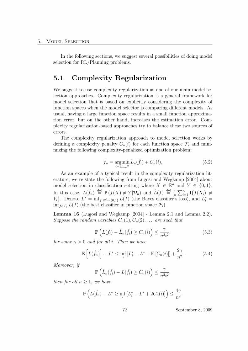
5. Model Selection

In the following sections, we suggest several possibilities of doing modelselection for RL/Planning problems.

5.1 Complexity Regularization

We suggest to use complexity regularization as one of our main model se-lection approaches. Complexity regularization is a general framework formodel selection that is based on explicitly considering the complexity offunction spaces when the model selector is comparing different models. Asusual, having a large function space results in a small function approxima-tion error, but on the other hand, increases the estimation error. Com-plexity regularization-based approaches try to balance these two sources oferrors.

The complexity regularization approach to model selection works bydefining a complexity penalty Cn(i) for each function space Fi and mini-mizing the following complexity-penalized optimization problem:

fn = argmini=1,...,P

Ln(fi) + Cn(i), (5.2)

As an example of a typical result in the complexity regularization lit-erature, we re-state the following from Lugosi and Wegkamp [2004] aboutmodel selection in classification setting where X ∈ Rd and Y ∈ 0, 1.In this case, L(fn)

def= P (f(X) 6= Y |Dn) and L(f)

def= 1

n

∑ni=1 If(Xi) 6=

Yi. Denote L∗ = inff :Rd 7→0,1 L(f) (the Bayes classifier’s loss), and L∗i =inff∈Fi

L(f) (the best classifier in function space Fi).

Lemma 16 (Lugosi and Wegkamp [2004] - Lemma 2.1 and Lemma 2.2).Suppose the random variables Cn(1), Cn(2), . . . are such that

P(L(fi)− Ln(fi) ≥ Cn(i)

)≤ γ

n2i2, (5.3)

for some γ > 0 and for all i. Then we have

E[L(fn)

]− L∗ ≤ inf

i[L∗i − L∗ + E [Cn(i)]] +

2γ

n2. (5.4)

Moreover, if

P(Ln(fi)− L(fi) ≥ Cn(i)

)≤ γ

n2i2,

then for all n ≥ 1, we have

P(L(fn)− L∗ ≥ inf

i[L∗i − L∗ + 2Cn(i)]

)≤ 4γ

n2.


Complexity Regularization

To give an intuition about this result, we note that for any fi ∈ Fi

minimizing the empirical loss Ln,

E[L(fi)

]− L∗ ≤

(inff∈Fi

L(f)− L∗)

+ E[(L− Ln)(fi)

], (5.5)

where the first term at the right hand side is the approximation error andthe second term is the estimation error.

The main idea behind complexity regularization is choosing a complex-ity term Cn(i) for Fi that is a tight upper bound for the estimation errorand meanwhile satisfies Eq. (5.3). Suppose for a moment that by select-

ing Cn(i) ≈ E[(L− Ln)(fi)

], the condition Eq. (5.3) is satisfied. Then

Eq. (5.4) implies that the difference between the loss of fn, which is theminimizer of Eq. (5.2), and the Bayes optimal loss L∗ is equal to the sum-mation of the estimation error and approximation error plus an additional2γn2 term. This latter term converges to zero quickly, so this result gives usan oracle-like inequality. Nonetheless, the right choice of Cn(i) can be diffi-cult as it should be a high probability tight upper bound on the estimationerror.

There are various approaches to designing a suitable Cn(i). Brieflyspeaking, there are two main approaches: (1) distribution-free and (2)data-dependent.

Distribution-free approaches to select Cn(i) use the distribution-freemeasures of the class complexity such as its VC dimension. Distribution-freemeasures of complexity, however, are too conservative, and do not providetight oracle-like guarantees.

The other possibility is to use a data-dependent complexity penaltyCn(i). These complexity penalties give tighter and less conservative per-formance bounds, and therefore lead to better and more accurate modelselection. These complexity penalties can be based on a hold-out set, em-pirical shatter coefficient, or Rademacher averages (see e.g. Bartlett et al.[2002]; Lugosi and Wegkamp [2004]).

To apply these ideas in RL/Planning context, we must find a result

similar to Lemma 16 that is suitable for our upper bound loss∥∥∥Q− T ∗Q

∥∥∥2

and its de-biased counterpart∥∥∥Q− T ∗Q

∥∥∥2

−∥∥∥h∗(Q)− T ∗Q

∥∥∥2

. This is not

a trivial task. Moreover, as discussed in the beginning of the chapter, theresult of this model selection approach only helps selecting the model withthe best upper bound.


5. Model Selection

5.2 Cross-Validation Methods

The other approach for model selection is to apply any method that uses asubset of samples for training and the remaining samples for model selection.This includes hold-out, n-fold cross-validation, and various bootstrappingmethods.

As discussed in Section 3.6, model selection is not very difficult forRFQI because it reduces to model selection for a sequence of regressionproblems, albeit one with dependent data in RL scenario. Therefore, amodel selection method such as an n-fold cross-validation may simply beused at each iteration of RFQI. Unfortunately, as far as we can tell, thereis no rigorous study which shows that even a simple n-fold cross-validationmethod works well in general and in the non-asymptotic regime. See Arlot[2008] for a discussion on n-fold cross-validation and its generalizations thathave desirable properties for histogram-based regression.

Model selection for REG-BRM and REG-LSTD is more complicated,mainly because we do not have an unbiased estimate of the surrogate loss∥∥∥Q− T ∗Q

∥∥∥2

, and we need to approximate it by∥∥∥Q− T ∗Q

∥∥∥2

−∥∥∥h∗(Q)− T ∗Q

∥∥∥2

.

The problem here is that we need this approximate loss converge to thesurrogate loss as quickly as possible, but this requires selecting h∗ from theright function space, which is itself unknown.

Although we might suggest using n-fold cross-validation or similar resampling-based methods for model selection in RL/Planning context, at least forRFQI, we do not analyze its properties in this work.

5.3 Dynamical System Learning for Model

Selection

If getting new samples are extremely cheap, we may directly estimate V πiρi

=Eρi

[V πi(X)] (Eq. (5.1)) by interacting with the environment and/or gettingsamples from the MDP, and use these estimates to provide ranking onmodels. This approach works by selecting initial states according to X0 ∼ ρi

and then running the MDP with the candidate policy πi, and measuringthe average of returns. Sampling from ρi can be done by a Markov ChainMonte Carlo (MCMC) approach (see e.g. Chapter 29 of MacKay [2003]).This Monte Carlo-style approach gives an estimate V πi

ρi,nMCthat converges

to V πiρi

with the rate O( 1√nMC

) where nMC is the number of trajectory runs.

This approach should work well when getting new samples, either byinteracting with the environment in the agent-environment scenario or using


Functional Estimation under Distribution Mismatch

MDP’s model, is cheap. If it is not, the following model selection proceduremay be applied:

For any MDP (X ,A, P,R), learn an approximate model (X ,A, Pn, Rn)using data samples. Now in order to select the best model (i.e. policy),instead of interacting with the environment, which we assume is not cheap,we use this learned model and invoke it to produce nMC virtual samples.Then we use those virtual samples to estimate the performance of eachgreedy action w.r.t. Q(i) for all i = 1, . . . , P . This gives us a set of V πi

ρi,nMC,

and so a ranking on all hypotheses.If P and R are close enough, in appropriate norms, to P and R, respec-

tively, we may expect that V(i)nMC is close to V πi

nMC, and so a ranking based

on these virtual samples is not totally off from the ranking based on realsamples.

It is not difficult to see that if we denote ∆R = R − R and ∆P π =P π− P π, the difference between the value function coming from the originalMDP and the approximate MDP can be written as

V π − V π = (I− γP π)−1R− (I− γP π)−1(R+ ∆R)

≈ (I− γP π)−1∆R+ γ∆PR.

This shows that whenever ∆R and ∆P are small, the error between V π

and V π will be small.Learning P and R are instances of supervised learning problems (con-

ditional density estimation and regression, respectively). Nevertheless, thisproblem is not as easy as it seems. We discuss this issue in the next section.

5.4 Functional Estimation under

Distribution Mismatch

Learning can be difficult when there is a mismatch between the trainingsamples’ distribution ν and the evaluation distribution ρ. This can espe-cially be a serious concern in RL setting, because more often than not thesamples are generated by a behavior policy whose induced stationary dis-tribution is different from the distribution with which we want to measurethe performance. In this section, we consider the problem of functionalestimation under distribution mismatch, and show that even in this simpleproblem serious difficulties may arise.

The functional estimation under distribution mismatch problem is toevaluate Eµ2 [f(X)] when we have access to samples in the form of Dn =


5. Model Selection

(Xi, Yi = f(Xi)ni=1 where Xi ∼ µ1 and µ1 and f(·) are unknown. We wantto have an algorithm that based on Dn, and the knowledge of µ2, gives ahigh probability confidence on Eµ2 [f(X)]. We define a sound algorithm forthis problem as follows.

Definition 17 (Sound Algorithm). Algorithm Cn ← AQ(Dn, δ, µ2) that re-turns confidence set Cn is called a sound algorithm for the class of problemsQ = (µ1, µ2, f) : dµi

dλ> 0; i = 1, 2; |f | is bounded by a finite real number

(λ is the uniform measure) if for ∀δ > 0 it satisfies the following criteria:

• ∀n ≥ 1; P (Eµ2 [f(X)] /∈ Cn) ≤ δ,

• |Cn| → 0 (n→∞) almost surely.

The following negative result says that no matter which algorithm oneuses, there is a problem that the algorithm fails to be sound with highprobability.

Theorem 18 (Impossibility of Functional Estimation Under DistributionMismatch). For any deterministic algorithm AQ(Dn, δ, µ2), there exist a Qsuch that the algorithm is not sound for Q with probability at least 1− δ.

The source of the difficulty is the largeness of Q: one can always finda problem instance where samples Dn is not a good representative for µ2.Nonetheless, if we restrict the class of problems Q by assuming some regu-larities, such as similarity between µ1 and µ2 quantified by KL(µ1||µ2) orother distance measures, there might be hope to have a sound algorithm.

Studying other related problems under distribution mismatch is inter-esting too, and may bring us insight about the difficulty of RL problems.One such problem is providing a lower bound on ‖f(·)‖µ1

when we knowthe value of ‖f(·)‖µ2

. The importance of this lower bound in RL/Planningcontext can be appreciated if we consider f(·) = Q − T ∗Q, µ2 = ν (sam-pling distribution of Dn) and µ1 = ρ (the desired evaluation measure, e.g.stationary distribution of the optimal policy). Then this result says thateven if we minimize ‖Q− T ∗Q‖ν , the loss that we care about, ‖Q− T ∗Q‖ρ,is not smaller than a quantity that is related to ‖Q− T ∗Q‖ν and some no-tion of similarity between ρ and ν. One may interpret such as a result as atheoretical limitation on off-policy learning.

Application to Reinforcement Learning

The previous negative result has an important implication for model selec-tion in batch RL setting.


Functional Estimation under Distribution Mismatch

Consider a Markov Decision Process (MDP) and the set of policiesπipi=1 and a batch of data Dn coming from distribution ν. Distribution νis induced stationary distribution of the behavior policy πb.

The goal of model selection for RL/Planning problems is to choose apolicy that, with high probability, has the maximum V πi

ρi(see Eq. (5.1)).

In order to compare these policies and to select the best policy with highprobability, the algorithm needs to compare the confidence interval on eachV πi

ρi.We define a Sound RL/Planning Model Selection Algorithm as follows.

Definition 19 (Sound RL/Planning Model Selection Algorithm). Algo-rithm

π∗ ← A′Q(Dn, δ, (π1, ρ1), . . . , (πp, ρp))

that chooses the policy with highest expected return is called a sound algo-rithm for the class of joint sampling distribution and MDP problems

Q =

(Dn ∼ ν, (X ,A, P,R, γ)) :dν

dλ> 0;

dρi

dλ> 0 for i = 1 . . . , p;

|R| is bounded by a finite real number

,

if for ∀δ > 0 it satisfies

P(π∗ 6= argmaxi=1,...,pV

πiρi

)≤ δ; ∀n ≥ 1.

Definition 19 reflects our desideratum of having an algorithm

A′Q(Dn, δ, (π1, ρ1), . . . , (πp, ρp)),

that chooses the policy with highest expected return with probability atleast 1 − δ. This definition is indeed very similar to the definition of asound algorithm in Definition 17: the sampling distribution ν is the sameas µ1 in Definition 17, and ρis play the role of µ2 in the same definition.

The following result states that the problem of model selection forRL/Planning problems in the batch setting is at least as difficult as theproblem of functional estimation under distribution mismatch.

Corollary 20. For any deterministic algorithm

π∗ ← A′Q(Dn, δ, (π1, ρi), . . . , (πp, ρp)),

there exists an MDP and a sampling distribution belonging to the class ofproblems Q such that the algorithm is not sound with probability at least1− δ.


5. Model Selection

In practice, the problem can be even more difficult. When ρi is theinduced stationary distribution of πi, which is a reasonable choice for theevaluation policy, the knowledge of ρi is not available to the algorithm (asopposed to the knowledge of µ2 in Definition 17). Moreover, data Dn arenot necessarily independent in the RL setting.

In spite of this negative result, there might still be hope if there aresome regularities among policies, e.g. if the behavior policy is close to thetarget policies.


Appendix A

Supervised Learning

As discussed in Section 1.2, even though there are some key differences be-tween an RL/Planning and supervised learning, one can still gain insight bystudying supervised learning results. It is especially true when RL/Planningproblems have large state spaces X , which is the usual assumption in su-pervised learning setup. To see how supervised learning results may beinsightful for analyzing RL/Planning problems, we first show that super-vised learning is a special case of RL/Planning problems.

Consider a discounted MDP with γ = 0, so V π(x) = E [R(·|x, π(x))].Therefore the policy evaluation problem given i.i.d. samples

Dn = ((X1, π(X1), R1, X′1), . . . , (Xn, π(Xn), Rn, X

′n)),

where Rt ∼ R(·|Xt, π(Xt)), is to estimate V π that is close to V π. Thisproblem is equivalent to the traditional i.i.d. regression, to be preciselydefined in Section A.1, when regression function is E [R(·|x, π(x))]. Thisscenario is a special case of RL/Planning problem because (1) γ is set tobe zero and (2) samples are assumed to be i.i.d.

The supervised learning literature provides two types of insight:

• Provide lower bounds that relate the performance of any algorithmto the difficulty of the problem, and

• Inspire us to design RL/Planning algorithms than can benefit fromregularities of the problem.

Lower bound results relate the sample complexity of solving a regres-sion/classification/density estimation problem to some intrinsic complexitymeasures of that problem. Examples of complexity measures are the dimen-sion of the input space, the degree of sparsity of the target function (Lafferty

79

A. Supervised Learning

and Wasserman [2006]; Zhang [2009]), the smoothness of the target func-tion (Gyorfi et al. [2002]), the Vapnik-Chervonenkis (VC) dimension of thehypothesis space, global and local Rademacher complexity of the hypoth-esis space (Bartlett and Mendelson [2002]; Koltchinskii [2006]) and manyothers. Because RL/Planning problem is a more general problem than theregression, these lower bounds are also lower bounds for RL/Planning. Ofcourse, this subset-hood relation does not imply that RL/Planning prob-lems are strictly more difficult than regression problems.

The other way supervised learning literature may help is to inspire usto design flexible RL/Planning algorithms. There are already many flexibleand adaptive supervised learning algorithms that exploit different regular-ities of the problem in hand. The results of this inspiration are algorithmsintroduced in Chapter 3 and Chapter 4.

In the next section, we formulate the regression problem, the supervisedlearning setting that is most relevant to our way of formulating RL/Planningproblems, and after that in Section A.2 we state some lower bounds for re-gression. These lower bounds show that one cannot hope to achieve fastconvergence bounds when the problem is intrinsically difficult. Section A.3is devoted to regularities and discuss various types of them which are well-known in supervised learning literature. This section is an extension ofSection 1.2. Finally in Section A.4, we mention several common parametricand nonparametric algorithms for solving regression problems.

A.1 Regression Problem

Consider a pair of random variables (X,Y ) where X ∈ Rd and Y ∈ Rwith µXY (or simply µ) as their joint probability distribution. The goal ofregression is to find a function] f(x) that approximates the relation betweenY and X based on observation pairs Dn = (Xi, Yi)ni=1, where (X, Y ) ∼µXY .

The notion of approximation can be interpreted in different ways. Oneway is to define a norm, like Lp norm, between random variable Y (x) andfunction f(x), and then finding a f(·) that minimizes a risk function[al]defined based on that norm. Lp-Risk is defined as

‖f(X)− Y ‖p,µ = E [|f(X)− Y |p]1p =

[∫X×Y

|f(x)− y|pµXY (dxdy)

] 1p

.

(A.1)If one choose L2 norm, it can be shown that the minimizer of L2 risk

is the conditional mean of Y w.r.t. X, i.e. r(x) = E [Y |X = x]. This


Lower Bounds for Regression

function is usually called the regression function. From now on, we assumewe are dealing with L2-risk and we simply denote it as ‖f(X)− Y ‖µ oreven ‖f(X)− Y ‖ if the underlying distribution is clear from the context,or is irrelevant in the discussion.

In most cases, we do not have access to the joint distribution, thereforewe cannot calculate the minimizer of the risk functional to get r(·). Instead,we may use samples Dn = (Xi, Yi)ni=1 ∼ µXY to provide rn(·;Dn) thatis close to r(·), where the notion of closeness is usually considered to beL2-Risk (but the use of other risks is possible).

For more information on regression, consult standard textbooks suchas Gyorfi et al. [2002] and Hastie et al. [2001].

A.2 Lower Bounds for Regression

Lower bounds (also called Slow Rates) provide insight about the intrinsicdifficulty of learning problems. They show how many samples are requirewhen we want to estimate the regression function/classifier/density/valuefunction up to a specific accuracy. These results are interesting becausethey demonstrate the intrinsic difficulty of learning problems – as opposedto the performance of a particular algorithm. Designing a method thatcan actually solve those problems is another issue, which we discuss inSection A.4.

The general result is that learning can be hopelessly difficult, unlessthere are some intrinsic regularities in the problem. If there are, we mayhope to exploit them and get reasonable performance. We talk about thisissue in more details in Section A.3.

The following theorem states that one may design a joint distributionµXY in such a way that the convergence rate of rn(·;Dn) toward r(·) isarbitrarily slow.

Theorem 21 (Gyorfi et al. [2002] – Theorem 3.1). Let an be a sequenceof positive numbers converging to zero. For every fixed sequence of regres-sion estimates rn(·;Dn), there exists a distribution µXY , such that X isuniformly distributed on [0, 1], Y = r(X) = ±1, and

lim supn→∞

E[‖rn − r‖2

]an

≥ 1.

This theorem states that for a subset of all regression problems, whereX is distributed uniformly and Y is noiseless samples that can be either +1or −1, the convergence rate can be arbitrary slow.



This result shows that we cannot hope to have a universal regressionmethod that performs well for all problems. Nevertheless, if we restrictthe range of problems µXY to a subset of joint distributions with certainamount of structure/regularities, we may hope to get better bounds.

To give an example of such a result, let us define the class of (p, C)-smooth functions:

Definition 22 ((p, C)-smoothness; Gyorfi et al. [2002] – Definition 3.3).Let p = k + β for some k ∈ N0 and 0 < β ≤ 1, and let C > 0. A functionf : Rd −→ R is called (p, C)-smooth if for every α = (α1, . . . , αd), αi ∈ N0,∑d

i=1 αi = k, the partial derivative ∂kf

∂xα11 ...∂x

αdd

exists and satisfies∣∣∣∣ ∂kf

∂xα11 . . . ∂xαd

d

(x)− ∂kf

∂xα11 . . . ∂xαd

d

(z)

∣∣∣∣ ≤ C ‖x− z‖β ,

for x, y ∈ Rd. Define F (p,C) to be the set of all (p, C)-smooth functionsf : Rd −→ R.

Let us define the class of regression problems where X comes from theuniform distribution on [0, 1]d, Y (x) − r(x) is a Gaussian random variable(so this is not noiseless anymore), and r(·) is (p, C)-smooth.

Definition 23 (D(p,C)). Let D(p,C) be the class of regression problems suchthat:

• X is uniformly distributed on [0, 1]d,

• Y = r(X) + η, where X and η are independent and η is a standardnormal random variable,

• r ∈ F (p,C).

Now we can state the main theorem regarding the lower bound conver-gence rate for D(p,C) and, therefore all regression problems with regressionfunction r(·) belonging to F (p,C).

Theorem 24 (Minimax and Individual Lower Bounds for D(p,C)). For theclass D(p,C), we have

lim infn→∞

infrn

sup(X,Y )∈D(p,C)

E[‖rn − r‖2

]≥ BC

2d2p+d n−

2p2p+d ,

for some constant B independent of C. This is called the lower minimaxbound of convergence.


On Regularities

Moreover, consider bn as an arbitrary positive sequence tending tozero. Then for the class D(p,C) we have

infrn

sup(X,Y )∈D(p,C)

lim supn→∞

E[‖rn − r‖2

]> bnn

− 2p2p+d .

which is called the individual lower bound of convergence.

A.3 On Regularities

The results of Section A.2 show that solving a regression problem mightnot be possible unless there is some underlying regularity in the problem.In that case, it is desirable to we have an algorithm that can automaticallydetect the right type of the regularity and exploit it. Such an algorithm iscalled adaptive.

There are several well-known types of regularities such as

• Smoothness

• Sparsity

• Low-Dimensionality of the Data Manifold

• Low Noise Margin Condition

Smoothness is one of the most common ways to discuss the regularityof a problem. There are various notions of smoothness, such as the (p, C)-smoothness that we previously defined (Definition 22). Indeed smoothnessis a more general concept. The way smoothness is used in Sobolev spacesare more general than (p, C)-smoothness defined before, and allows havingsmooth functions with occasional discontinuities, see Triebel [2006, Chapter1: How to Measure Smoothness] for a general treatment of this topic.

Sparsity is another type of regularity that recently has attracted consid-erable attention. Consider a p-dimensional function space F with Φipi=1

as its basis functions. Therefore, any function f ∈ F can be written asf(·) =

∑pi=1 wiΦi(.). A function f is said to be s-sparse when the number

of non-zero wis is s, i.e. s = |wi 6= 0 : i = 1, . . . , p|. If we know that weare dealing with sparse functions, we may exploit it. See Section 2 of Laf-ferty and Wasserman [2006] for an early survey and discussion on sparsity,and Zhang [2009] for analysis of benefiting from sparsity in the regressioncontext.

Low-dimensionality of data manifold is a geometrical regularity describ-ing the situation that input data come from a D-dimensional space X but



they are confined on (or close to) d-dimensional manifold M ⊂ X . Wecall an algorithm manifold-adaptive if it can exploit this property andperform as if the dimension of the input space is d. This leads to a hugegain whenever d D.

Recently, there have been a few theoretical results that show the pos-sibility of having manifold-adaptive algorithms. Farahmand et al. [2007b]shows that the sample complexity of estimating the dimension of manifolddepends mainly on the intrinsic dimension of manifold and not the dimen-sion of the embedding space. Farahmand et al. [2007c] present a resultthat shows that a simple K-nearest neighborhood regression algorithm isindeed manifold-adaptive (of course, K-nearest neighborhood does not ex-ploit other regularities of the problem such as its smoothness). See thework of Farahmand et al. [2009e] for more detail about this work. Amongother work that prove manifold-adaptivity, we can refer to Scott and Nowak[2006] that introduces dyadic decision trees for classification. Another ap-proach with favorable manifold-adaptive properties is Random ProjectionTree (Dasgupta and Freund [2008]) which is a variant of k-d trees. It usesrandom splitting directions instead of splitting along a coordinate directionand adds randomness to the median as a point of splitting.

Nevertheless, to the best of our knowledge, we are far from a generalstatistical theory of manifold-adaptive algorithms.

Margin condition (or low noise condition) is another type of regularitythat appears in classification problems. It talks about the behavior of aposteriori probability function η(x) = P (Y = 1|X = x) around the criticaldecision point 1

2. If η(x) is far away from 1

2(by having a gap as described

by Massart’s noise condition or decaying fast when it get close to 12, which

is called Tsybachov’s noise condition), the classification problem becomeseasier and one can show that the convergence rate would be much faster.See Tsybakov [2004] and Section 5.2 of Boucheron et al. [2005].

Of course, our short discussion should not imply that these are the onlypossible regularities one may exploit in a given problem. There are severalother types of regularities that explicitly or implicitly have been discussed inthe machine learning and/or statistics literature (e.g. ANOVA decompos-ability). One can be sure that there will be many undiscovered regularitiesin real-world learning problems that might be useful to be considered whendesigning a machine learning algorithm.


Algorithms for Regression Problems

A.4 Algorithms for Regression Problems

In Section A.2, we discussed lower bounds and the intrinsic difficulty ofmachine learning problems and, in particular, we reviewed some resultsfrom the regression literature. A natural question is whether there is anyalgorithm that can actually perform reasonably well and has upper samplecomplexity bound that matches or at least is close to the lower bound.

The goal of this section is to provide a brief overview of several regressionalgorithms. The literature on supervised learning in general and regressionin particular is abundant and there are many algorithms with various desir-able properties. Moreover, some of them even behave optimally for certaintypes of regularities. For more information, refer to standard textbookssuch as Hastie et al. [2001] and Bishop [2006] for algorithmic coverage andDevroye et al. [1996], Gyorfi et al. [2002], and Wasserman [2007] for moretheoretical analysis.

One way to categorize machine learning/statistics algorithms is whetherthey are parametric or nonparametric. Parametric methods are thosethat try to find the estimate (e.g. the estimated regression function/classifier)from a finite dimensional function space, while nonparametric methods arethose that can potentially use an infinite dimensional function space.

If we know that the target function belongs to the selected finite dimen-sional function space, parametric methods usually provide more accurateestimates given some fixed number of data samples. Nevertheless, if thefunction space is not expressive enough to include the target function, theresult can be horrendously bad. A simple example of this situation is whenwe want to learn a regression function r(x) = sin(x), but we are restrictedto function space of the form F = θ · x|x ∈ R, θ ∈ R. Briefly speaking,parametric models result in a small estimation error, but if the choice of thefunction space is incorrect, they may have a large function approximationerror. This may happen if the designer does not have sufficient knowledgeof the target function, which is not unusual.

Nonparametric methods are generally working with larger function spaces.In many cases, that function space can be even infinite dimensional. Be-cause of that, they are more expressive and can potentially approximateany ”reasonable” function arbitrary well.1 Conversely, working with a verylarge function space without extra care may lead to large estimation errors.

1We use the term reasonable vaguely, but one may consider that we are talking aboutpiecewise continuous functions.



Parametric Approaches

A simple parametric approach to regression (or classification) is to use Lin-ear Models. Here we assume that r(x) can be written as r(x) = xT θ, whereθ ∈ Rd. For linear models, we write the regression function as a linear com-bination of basis functions in the form of xidi=1 where x = (x1 · · ·xd)

T .Then the problem of finding regression function can be formulated as thefollowing empirical risk minimization problem with L2 risk:

θ ← arg minθ

n∑i=1

(XTi θ − Yi)

2 = arg minθ

∥∥XT θ −Y∥∥2

, (A.2)

where X is d × n matrix where its ith column represents the ith datasample, and Y is the n-dimensional vector that consists of all the re-sponses. This optimization problem has a closed-form solution of the formθ0 = (XXT )−1XY whenever XXT is invertible. This estimate is sometimescalled Ordinary Least Squares (OLS) estimate. For more information aboutlinear models, see Chapter 3 of Hastie et al. [2001].

It is apparent that many phenomena cannot be described by simplelinear models. A trivial extension of linear models is called General LinearModels. The basic idea of general linear models is to introduce new basisfunctions based on the original input features and represent the regressionfunction as the linear combination of these new basis functions. Here wewrite r(·) ∈ Fp = φ(x)T θ|θ ∈ Rp, φ(·) : Rd 7→ Rp. If p = d and φi(x) = xi

(i = 1, . . . , d), the result is reduced to the basic linear model.In practice, one may want to build a large dictionary of basis functions

(p d) in order to add flexibility to the class of functions the algorithmcan approximate. This may happen, for example, if we want to use apolynomial of degree two to approximate the desired function. This meansthat we have the set of x1, . . . , xd ∪ xixji,j=1,...,d as our basis functions,which has p = O(d2) terms. The difference between p and d can be moredramatic when one uses over-complete dictionaries such as wavelets thathas multiple resolutions of basis expansion.

The result of basis expansion is increasing the size of the function space.This helps reducing the function approximation error but may increase theestimation error. This is sometimes called overfitting. With some stan-dard assumptions on the problem (like finiteness of bound on |r(X)| andσ(Y |X = x)), the L2 excess risk ‖rn − r‖2 behaves as follows (Theorem11.3 of Gyorfi et al. [2002]):

C1

(p log(n)

n

)+ C2

(inf

f∈Fp

‖(f(X)− r(X)‖2µX

), (A.3)



with universal C1, C2 > 0.

The first term shows the effect of the estimation error (variance). Thisterm has a linear dependence on the size of feature space p, so one can saythat adding more basis to the set of features increases the estimation error.Conversely, the second term, the approximation error (bias), decreases whenwe enrich the feature space. The function approximation error shows theminimum error we would suffer by limiting ourself to function space Fp. Ingeneral, by increasing the size (or capacity) of Fp, this error will decrease.

When the designer is not sure about the right form of the target func-tion, he may define a family of function spaces, from simple to complex,and explicitly or implicitly use model selection to select between them. Forexample, he may select a subset of all features, and then use them as fea-tures of a standard linear model method (see Section 3.4.1 of Hastie et al.[2001]). Trying to select the best set of features, in general, is a difficultcombinatorial optimization problem and cannot be efficiently solved. Usualsubset selection methods like forward stepwise selection or backward step-wise selection add/eliminate new features greedily. Because of that, it isquite possible that they do not select the best subset of all features. Thismakes them suboptimal.

Another alternative is using regularization (penalization) and/orshrinkage. In regularization, one restricts the search to a subset of allpossible functions in the function space. In the parametric case, one restrictsthe weight vector w. This reduces the size of function space, and thus itscomplexity. By decreasing the function space’s complexity, the estimationerror decreases. On the other hand, the expressibility of functions in thatspace decreases too. This leads to a potential increase in the functionapproximation error. By choosing the right amount of regularization, wemay balance these two sources of errors and maximizes the generalizationperformance.

Two common regularization methods in parametric regression are theridge regression and LASSO.

The ridge regression is defined by the following optimization problem:

θ ← arg minθ

n∑i=1

(XTi θ − Yi)

2 + λn ‖θ‖22 ≡ arg minθ

∥∥XT θ −Y∥∥2

+ λn ‖θ‖22 .

(A.4)



Equivalently, the ridge regression can also be formulated as

θ ← arg minθ

n∑i=1

(XTi θ − Yi)

2, (A.5)

s.t. ‖θ‖22 ≤ µn,

where there is a one-to-one data-dependent correspondence between λn andµn, i.e. for any choice of λn, and Dn = (Xi, Yi)ni=1, there exists a µn wherethe solutions of Eq. (A.4) and Eq. (A.5) are the same, and vice versa.

Based on the formulation, one can see that the ridge regression penal-izes l2 norm of weights, and favors solutions with smaller l2 norm. Min-imizing some form of L2 norm is a common way of regularization. LikeOLS, the ridge regression has a closed-form solution which is θridge =(XXT + λnI)

−1XY, where I is an p× p identity matrix.LASSO (Least Absolute Shrinkage and Selection Operator) is another

regularized regression method for parametric models that constrains l1 normof weights.

θ ← arg minθ

n∑i=1

(XTi θ − Yi)

2, (A.6)

s.t. ‖θ‖1 ≤ µn,

where ‖θ‖1 =∑p

i=1 |θi| for p-dimensional θ.LASSO does some sort of soft shrinkage on weights. When µn is small,

some of the weights might become exactly zero. This is the model selectionproperty of LASSO that has attracted much attention.

To understand the shrinkage property of LASSO, and to compare itwith what the ridge regression does, let us consider the situation whereXXT = I. One can show that the solution of LASSO (Eq. (A.6)) will be

θ(LASSO)i = sign(θ0

i )(|θ0i − γ|)+ where θ0 is the solution of OLS defined in

Eq. (A.2), and γ is some value that depends on µn. Here (α)+ return thevalue of α if α is positive and returns 0 if it is non-positive. So if someof components of the weight vector of the original OLS is smaller than athreshold, it will be cut to zero. Other values would shrink toward zero,and the transition is continuous. The ridge regression, however, returnsθ

(ridge)i = 1

1+λθ0

i . It always shrinks values toward zero, but there is nozeroing effect. This means that the result of LASSO can possibly be sparse,while the result of the ridge regression is not sparse in general. This makesLASSO more appealing that the ridge regression whenever the data can bedescribed by only a few of input variables, e.g. when many dimensions ofX ∈ Rd are irrelevant.



Nonparametric Approaches

There are many nonparametric methods for regression, classification, anddensity estimation. Examples are K-Nearest Neighborhood regression, smooth-ing kernel regression, locally linear regression, additive models such asregression trees, boosting, dictionary-based models such as those usingwavelets as basis functions and some form of shrinkage for parameters es-timation, margin maximizing methods like Support Vector Machines withkernels, artificial neural networks such as MLP and RBF, and regularizedleast squares methods (Devroye et al. [1996]; Hastie et al. [2001]; Gyorfiet al. [2002]; Bishop [2006]; Rasmussen and Williams [2006]; Wasserman[2007]).

For instance, the regularized (penalized) least squares method is anonparametric counterpart of the ridge regression. It uses a general functionspace F , and use the norm of that space as the regularizer. If that functionspace is a Sobolev space and the regularizer is the corresponding Sobolevspace norm, the result is called thin plate splines. More generally, we canformulate the regularized least squares problem in a reproducing kernelHilbert space (RKHS) with the corresponding norm ‖·‖H as regularizer.

The regularized least squares has a Bayesian interpretation: in the Gaus-sian Processes regression setting, choose the covariance kernel the same asthe RKHS kernel, and select the maximum of the posterior distributionafter observing data. The selected function is the same as the solution ofregularized least squares with the same kernel function (Rasmussen andWilliams [2006]).

The regularized least squares-based methods is the inspiring approachthat we use in this project to design nonparametric RL/Planning algorithms(Chapter 3 and Chapter 4).


Appendix B

Mathematical Background

Function Spaces

Definition 25. A function f : X 7→ R for X ⊂ Rd is Holder continuous if

|f(x)− f(y)| ≤ C|x− y|α (x, y ∈ X ),

for nonnegative finite real number C and α.

Definition 26. The Holder space Cα,k(X ) is the space of all functions withdomain Ω that their derivatives up to order k, an integer number, are Holdercontinuous with 0 < α ≤ 1.

Definition 27 (Sobolev Space Wk,p(X ) – Devore [1998]). Let k be a non-negative integer number and 1 ≤ p ≤ ∞. The Sobolev space Wk,p(X ) foropen and connected subset X ⊂ Rd is the space of all measurable functionswhose distributional derivative of order k is in Lp, i.e.

∥∥∥∥ ∂|α|f

∂xα11 . . . ∂xαd

d

∥∥∥∥Lp(X )

≤ ∞,

for every multi-index |α| ≤ k. The semi-norm for Wk,p(X ) is defined as

|f |Wk,p(X )def=∑|α|=k

∥∥∥∥ ∂|α|f

∂xα11 . . . ∂xαd

d

∥∥∥∥Lp(X )

,

and their norm by ‖f‖Wk,p(X )

def= |f |Wk,p(X ) + ‖f‖Lp(X ).

91

B. Mathematical Background

In this work, we denote Wk(Rd)def= Wk,2(Rd).

Sobolev spaces generalize Holder spaces by allowing functions which areonly almost everywhere differentiable.

Another relevant class of function spaces is the Besov space Bsp,q(X )

for 0 < p, q ≤ ∞ and s > 0 which generalizes Sobolev spaces by letting0 < p < 1 and having fractional smoothness order s. For instance, Bs

2,2(Rd)is the same as Wk(Rd). We do not define Besov spaces here, and onlymention that Besov spaces can be defined with the help of modulus ofsmoothness. See Devore [1998] for more information.

Fixed-Point Theorems

Theorem 28 (Banach Fixed-Point Theorem - Hutson et al. [2005]). Let(X , d) be a non-empty complete metric space. Let L : X 7→ X be a contrac-tion mapping on X . Then the map L admits a unique fixed point f ∗ = Lf ∗

with f ∗ ∈ X . The fixed point can be find by iterative application of L onarbitrary f0 ∈ X , i.e., f ∗ = limk→∞ Lkf0.


List of Symbols

MDP

X : State space

A: Action space – A finite set with cardinality M

X ×A: State-Action space

P : X ×A →M(X ): Transition probability kernel

R: Reward distribution

γ: Discount factor

π: Policy

V π(·): Value function for policy π

Qπ(·): Action-value function for policy π

V ∗(·): Optimal value function

Q∗(·): Optimal action-value function

π(·; Q): Greedy policy w.r.t. the action-value function Q

T π: Bellman operator

T ∗: Bellman optimality operator

T π: Empirical Bellman operator

T ∗: Empirical Bellman optimality operator

Function Spaces

F : A subset of measurable functions X 7→ R.

93

B. Mathematical Background

FM : the subset of multi-valued measurable functions X ×A → RM .

H: RKHS. It is used instead of FM in optimization problems when we wantto emphasize the problem is formulated for an RKHS.

Wk(Rd): Sobolev space Wk,2(Rd).

‖f‖ν:∫X |f(x)|2dν(x)

‖f‖ν,n:1n

∑nt=1 f 2(Xt) , Xt ∼ ν.

J(Q): Regularizer/Penalizer of Q.

Jk(Q): Norm of Q in Wk(Rd).

Sampling

X ∼ P : X is a sample from distribution P .

Dn = (X1, A1, R1, X′1), . . . , (Xn, An, Rn, X

′n): Data samples used for RFQI,

REG-LSTD, and REG-BRM

ν: Distribution underlying (Xt, At).

νX : State-marginal distribution of Xt.

mk and nk: In the kth iteration of RFQI, we use mk samples with indexnk ≤ i < nk + mk = nk+1 − 1.

Others

Θ(·): Θ(f(n)) = g(n) : ∃c1, c2 > 0 and n0 s.t. 0 ≤ c1g(n) ≤ f(n) ≤c2g(n) for n ≥ n0

∆π: ∆π : X ×A 7→ [0, 1] is a function of state and action with the propertythat

∑Mi=1 ∆π(x, ai) ≤ 1 for all x ∈ X .

B(c)(= B(c, ‖·‖)): f ∈ F| ‖f‖ ≤ c


Bibliography

Andras Antos, Remi Munos, and Csaba Szepesvari. Fitted Q-iteration incontinuous action-space MDPs. In J.C. Platt, D. Koller, Y. Singer, andS. Roweis, editors, Advances in Neural Information Processing Systems(NIPS - 20), pages 9–16, Cambridge, MA, 2008a. MIT Press.

Andras Antos, Csaba Szepesvari, and Remi Munos. Learning near-optimalpolicies with Bellman-residual minimization based fitted policy iterationand a single sample path. Machine Learning, 71:89–129, 2008b.

Sylvain Arlot. V-fold cross-validation improved: V-fold penalization. Tech-nical report, Willow Team, CNRS, 2008.

Peter Auer, Thomas Jaksch, and Ronald Ortner. Near-optimal regretbounds for reinforcement learning. In D. Koller, D. Schuurmans, Y. Ben-gio, and L. Bottou, editors, Advances in Neural Information ProcessingSystems 21, pages 89–96, 2009.

Leemon Baird. Residual algorithms: Reinforcement learning with functionapproximation. In In Proceedings of the Twelfth International Conferenceon Machine Learning, pages 30–37. Morgan Kaufmann, 1995.

Peter L. Bartlett and Shahar Mendelson. Rademacher and Gaussian com-plexities: Risk bounds and structural results. Journal of Machine Learn-ing Research, 3:463–482, 2002.

Peter L. Bartlett, Stephane Boucheron, and Gabor Lugosi. Model selectionand error estimation. Machine Learning, 48(1-3):85–113, 2002.

Jonathan Baxter and Peter L. Bartlett. Innite-horizon policy-gradient esti-mation. Journal of Artificial Intelligence Research, pages 319–350, 2001.

Dimitri P. Bertsekas and Steven E. Shreve. Stochastic Optimal Control:The Discrete-Time Case. Academic Press, 1978.

95

Bibliography

Dimitri P. Bertsekas and John N. Tsitsiklis. Neuro-Dynamic Programming(Optimization and Neural Computation Series, 3). Athena Scientific,1996.

Aude Billard, Sylvain Calinon, Rudiger Dillmann, and Stefan Schaal. Robotprogramming by demonstration. In Siciliano and Khatib [2008], pages1371–1394.

Christopher M. Bishop. Pattern Recognition and Machine Learning.Springer, 2006.

Stephane Boucheron, Olivier Bousquet, and Gabor Lugosi. Theory of clas-sification: A survey of some recent advances. ESAIM: Probability andStatistics, 9:323–375, 2005.

Steven J. Bradtke and Andrew G. Barto. Linear least-squares algorithmsfor temporal difference learning. Machine Learning, 22:33–57, 1996.

Cynthia Breazeal, Atsuo Takanishi, and Tetsunori Kobayashi. Social robotsthat interact with people. In Siciliano and Khatib [2008], pages 1349–1369.

Jeffrey B. Burl. Linear Optimal Control: H2 and H∞ Methods. Addison-Wesley Longman Publishing Co., Inc., Boston, MA, USA, 1998.

Francois Chaumette and Seth Hutchinson. Visual servoing and visual track-ing. In Siciliano and Khatib [2008], pages 563–583.

Henrik I. Christensen and Gregory D. Hager. Sensing and estimation. InSiciliano and Khatib [2008], pages 87–107.

Fan R. K. Chung. Spectral Graph Theory (CBMS Regional ConferenceSeries in Mathematics, No. 92). American Mathematical Society, 1997.

Gerda Claeskens and Nils Lid Hjort. Model Selection and Model Averaging.Cambridge University Press, 2008.

Mark R. Cutkosky, Robert D. Howe, and William R. Provancher. Forceand tactile sensors. In Siciliano and Khatib [2008], pages 455–476.

Kostas Daniilidis and Jan-Olof Eklundh. 3-D vision and recognition. InSiciliano and Khatib [2008], pages 543–562.

Sanjoy Dasgupta and Yaov Freund. Random projection trees and low di-mensional manifolds. In Proceedings of ACM Symposium on Theory ofComputing (STOC), pages 537–546. ACM, 2008.


Daniela Pucci de Farias and Benjamin Van Roy. On the existence of fixedpoints for approximate value iteration and temporal-difference learning.Journal of Optimization Theory and Application, 105(3):589–608, 2000.

Ronald A. Devore. Nonlinear approximation. Acta Numerica, 7:51–150,1998.

Luc Devroye, Laszlo Gyorfi, and Lugosi Gabor. A Probabilistic Theory ofPattern Recognition. Applications of Mathematics: Stochastic Modellingand Applied Probability. Springer-Verlag New York, 1996.

Paul Doukhan. Mixing: Properties and Examples, volume 85 of LectureNotes in Statistics. Springer-Verlag, Berlin, 1994.

Yaakov Engel, Shie Mannor, and Ron Meir. Reinforcement learning withGaussian processes. In ICML ’05: Proceedings of the 22nd internationalconference on Machine learning, pages 201–208. ACM, 2005.

Damien Ernst, Pierre Geurts, and Louis Wehenkel. Tree-based batch modereinforcement learning. Journal of Machine Learning Research, 6:503–556, 2005.

Amir-massoud Farahmand, Azad Shademan, and Martin Jagersand. Globalvisual-motor estimation for uncalibrated visual servoing. In IEEE/RSJInternational Conference on Intelligent Robots and Systems, pages 1969–1974. IEEE, 2007a.

Amir-massoud Farahmand, Csaba Szepesvari, and Jean-Yves Audibert.Manifold-adaptive dimension estimation. In ICML ’07: Proceedings ofthe 24th international conference on Machine learning, pages 265–272,New York, NY, USA, 2007b. ACM.

Amir-massoud Farahmand, Csaba Szepesvari, and Jean-Yves Audibert. To-ward manifold-adaptive learning. In NIPS Workshop on Topology learn-ing, Whistler, Canada, December 2007c.

Amir-massoud Farahmand, Mohammad Ghavamzadeh, Csaba Szepesvari,and Shie Mannor. Regularized fitted Q-iteration: Application to plan-ning. In Sertan Girgin, Manuel Loth, Remi Munos, Philippe Preux, andDaniil Ryabko, editors, Recent Advances in Reinforcement Learning, 8thEuropean Workshop, EWRL 2008, volume 5323 of Lecture Notes in Com-puter Science, pages 55–68. Springer, 2008.


Bibliography

Amir-massoud Farahmand, Mohammad Ghavamzadeh, Csaba Szepesvari,and Shie Mannor. Regularized fitted Q-iteration for planning incontinuous-space markovian decision problems. In Proceedings of Amer-ican Control Conference (ACC), pages 725–730, June 2009a.

Amir-massoud Farahmand, Mohammad Ghavamzadeh, Csaba Szepesvari,and Shie Mannor. Regularized policy iteration. In D. Koller, D. Schuur-mans, Y. Bengio, and L. Bottou, editors, Advances in Neural InformationProcessing Systems 21, pages 441–448. MIT Press, 2009b.

Amir-massoud Farahmand, Majid Nili Ahmadabadi, Babak N. Araabi, andCaro Lucas. Interaction of culture-based learning and cooperative co-evolution and its application to automatic behavior-based system design.IEEE Transactions on Evolutionary Computation (accepted for publica-tion), 2009c.

Amir-massoud Farahmand, Azad Shademan, Martin Jagersand, and CsabaSzepesvari. Model-based and model-free reinforcement learning for visualservoing. In Proceedings of IEEE International Conference on Roboticsand Automation (ICRA), pages 2917–2924, May 2009d.

Amir-massoud Farahmand, Csaba Szepesvari, and Jean-Yves Audibert.Nearest neighborhood methods for manifold-adaptive dimension estima-tion and regression. under preparation, 2009e.

Dario Floreano, Phil Husbands, and Stefano Nolfi. Evolutionary Robotics.In Siciliano and Khatib [2008], pages 1423–1451.

Jurgen Forster and Manfred K. Warmuth. Relative loss bounds fortemporal-difference learning. Machine Learning, 51(1):23–50, 2003.

Alborz Geramifard, Michael Bowling, Michael Zinkevich, and Richard S.Sutton. iLSTD: Eligibility traces and convergence analysis. InB. Scholkopf, J. Platt, and T. Hoffman, editors, Advances in Neural In-formation Processing Systems 19, pages 441–448. MIT Press, Cambridge,MA, 2007.

Mohammad Ghavamzadeh and Yaakov Engel. Bayesian actor-critic algo-rithms. In Zoubin Ghahramani, editor, Proceedings of the 24th AnnualInternational Conference on Machine Learning (ICML 2007), pages 297–304. Omnipress, 2007a.

Mohammad Ghavamzadeh and Yaakov Engel. Bayesian policy gradientalgorithms. In B. Scholkopf, J. Platt, and T. Hoffman, editors, Advances


in Neural Information Processing Systems 19, pages 457–464. MIT Press,Cambridge, MA, 2007b.

Laszlo Gyorfi, Michael Kohler, Adam Krzyzak, and Harro Walk. ADistribution-Free Theory of Nonparametric Regression. Springer Verlag,New York, 2002.

Trevor Hastie, Robert Tibshirani, and Jerome Friedman. The Elements ofStatistical Learning: Data Mining, Inference, and Prediction. Springer,2001.

Vivian Hutson, John Sydney Pym, and Michael J. Cloud. Applicationsof Functional Analysis and Operator Theory (Second Edition). Elsevier,2005.

Tobias Jung and Daniel Polani. Least squares SVM for least squares TDlearning. In In Proc. 17th European Conference on Artificial Intelligence,pages 499–503, 2006.

Sham Kakade. A natural policy gradient. In NIPS, pages 1531–1538, 2001.

Charles C. Kemp, Paul Fitzpatrick, Hirohisa Hirukawa, Kazuhito Yokoi,Kensuke Harada, and Yoshio Matsumoto. Humanoids. In Siciliano andKhatib [2008], pages 1307–1333.

Hassan K. Khalil. Nonlinear Systems (3rd Edition). Prentice Hall, 2001.

J. Kivinen, A.J. Smola, and R.C. Williamson. Online learning with kernels.Signal Processing, IEEE Transactions on, 52(8):2165–2176, Aug. 2004.

Vladimir Koltchinskii. 2004 ims medallion lecture: Local Rademachercomplexities and oracle inequalities in risk minimization. ANNALS OFSTATISTICS, 34:2593–2656, 2006.

Vijay R. Konda and John N. Tsitsiklis. On actor-critic algorithms. SIAMJournal on Control and Optimization, pages 1143–1166, 2001.

David Kortenkamp and Reid G. Simmons. Robotic systems architecturesand programming. In Siciliano and Khatib [2008], pages 187–206.

John Lafferty and Larry Wasserman. Challenges in statistical machinelearning. Statistica Sinica, 16:307–322, 2006.

Michail G. Lagoudakis and Ronald Parr. Least-squares policy iteration.Journal of Machine Learning Research, 4:1107–1149, 2003.


Bibliography

Yuxi Li, Csaba Szepesvari, and Dale Schuurmans. Learning exercise policiesfor American options. In International Conference on Artificial Intelli-gence and Statistics (AISTATS-09), 2009.

Manuel Loth, Manuel Davy, and Philippe Preux. Sparse temporal differencelearning using LASSO. In IEEE International Symposium on Approxi-mate Dynamic Programming and Reinforcement Learning, 2007.

Gabor Lugosi and Marten Wegkamp. Complexity regularization via local-ized random penalties. Annals of Statistics, 32:1679–1697, 2004.

David J. C. MacKay. Information Theory, Inference, and Learning Algo-rithms. Cambridge University Press, 2003.

Sridhar Mahadevan and Mauro Maggioni. Proto-value functions: A Lapla-cian framework for learning representation and control in markov decisionprocesses. Journal of Machine Learning Research, 8:2169–2231, 2007.

Maja J. Mataric and Francois Michaud. Behavior-based systems. In Sicil-iano and Khatib [2008], pages 891–909.

Claudio Melchiorri and Makoto Kaneko. Robot hands. In Siciliano andKhatib [2008], pages 345–360.

Francisco Melo, Sean P. Meyn, and Isabel Ribeiro. An analysis of reinforce-ment learning with function approximation. In Andrew McCallum andSam Roweis, editors, Proceedings of the 25th Annual International Con-ference on Machine Learning (ICML 2008), pages 664–671. Omnipress,2008.

Ishai Menache, Shie Mannor, and Nahum Shimkin. Basis function adapta-tion in temporal difference reinforcement learning. Annals of OperationsResearch, 134(1):215–238, 2005.

Jean-Arcady Meyer and Agnes Guillot. Biologically inspired robots. InSiciliano and Khatib [2008], pages 1395–1422.

Sean P. Meyn. Control Techniques for Complex Networks. Cambridge, 2008.

Remi Munos. Performance bounds in lp norm for approximate value itera-tion. SIAM Journal on Control and Optimization, 2007.

Remi Munos and Csaba Szepesvari. Finite-time bounds for fitted valueiteration. Journal of Machine Learning Research, 9:815–857, 2008.


Yuriy Nevmyvaka, Yi Feng, and Michael Kearns. Reinforcement learningfor optimized trade execution. In ICML ’06: Proceedings of the 23rd in-ternational conference on Machine learning, pages 673–680. ACM, 2006.

Dirk Ormoneit and Saunak Sen. Kernel-based reinforcement learning. Ma-chine Learning, 49:161–178, 2002.

Ronald Parr, Christopher Painter-Wakefield, Lihong Li, and MichaelLittman. Analyzing feature generation for value-function approximation.In ICML ’07: Proceedings of the 24th international conference on Ma-chine learning, pages 737 – 744, New York, NY, USA, 2007. ACM.

Ronald Parr, Lihong Li, Gavin Taylor, Christopher Painter-Wakefield, andMichael Littman. An analysis of linear models, linear value-function ap-proximation, and feature selection for reinforcement learning. In ICML’08: Proceedings of the 25th international conference on Machine learn-ing, pages 752–759. ACM, 2008.

Jan Peters, Vijayakumar Sethu, and Stefan Schaal. Reinforcement learningfor humanoid robotics. In Humanoids2003, Third IEEE-RAS Interna-tional Conference on Humanoid Robots, 2003.

Marek Petrik. An analysis of Laplacian methods for value function ap-proximation in MDPs. In International Joint Conference on ArtificialIntelligence (ICAJ), pages 2574–2579, 2007.

Joelle Pineau, Marc G. Bellemare, A. John Rush, Adrian Ghizaru, andSusan A. Murphy. Constructing evidence-based treatment strategies us-ing methods from computer science. Drug and Alcohol Dependence, 88,supplement 2:S52-S60, 2007.

Erwin Prassler and Kazuhiro Kosuge. Domestic robotics. In Siciliano andKhatib [2008], pages 1253–1281.

Domenico Prattichizzo and Jeffrey C. Trinkle. Grasping. In Siciliano andKhatib [2008], pages 671–700.

Carl Edward Rasmussen and Christopher K. I. Williams. Gaussian Pro-cesses for Machine Learning. MIT Press, 2006.

Martin Riedmiller. Neural fitted Q iteration – first experiences with adata efficient neural reinforcement learning method. In 16th EuropeanConference on Machine Learning, pages 317–328, 2005.


Bibliography

Bernhard Scholkopf and Alexander J. Smola. Learning with Kernels. MITPress, Cambridge, MA, 2002.

Bernhard Scholkopf, Ralf Herbrich, and Alex J. Smola. A generalized rep-resenter theorem. In COLT ’01/EuroCOLT ’01: Proceedings of the 14thAnnual Conference on Computational Learning Theory and and 5th Eu-ropean Conference on Computational Learning Theory, pages 416–426.Springer-Verlag, 2001.

Paul J. Schweitzer and Abraham Seidmann. Generalized polynomial ap-proximations in Markovian decision processes. Journal of MathematicalAnalysis and Applications, 110:568–582, 1985.

Clayton Scott and Robert Nowak. Minimax-optimal classification withdyadic decision trees. IEEE Transactions on Information Theory, 52:1335–1353, 2006.

Bruno Siciliano and Oussama Khatib, editors. Springer Handbook ofRobotics. Springer, 2008.

David Silver, Richard S. Sutton, and Martin Muller. Reinforcement learn-ing of local shape in the game of go. In Manuela M. Veloso, editor,International Joint Conference on Artificial Intelligence (IJCAI), pages1053–1058, 2007.

Steve Smale and Ding-Xuan Zhou. Estimating the approximation error inlearning theory. Analysis and Applications, 1(1):17–41, 2003.

Richard S. Sutton and Andrew G. Barto. Reinforcement Learning: AnIntroduction (Adaptive Computation and Machine Learning). The MITPress, 1998.

Csaba Szepesvari. Static and Dynamic Aspects of Optimal Sequential De-cision Making. PhD thesis, Bolyai Institute of Mathematics, Universityof Szeged, Szeged, Aradi vrt. tere 1, HUNGARY, 6720, September 1997.

Gavin Taylor and Ronald Parr. Kernelized value function approximationfor reinforcement learning. In ICML ’09: Proceedings of the 26th AnnualInternational Conference on Machine Learning, pages 1017–1024, NewYork, NY, USA, 2009. ACM.

Gerald Tesauro. TD-gammon, a self-teaching backgammon program,achieves master-level play. Neural Computation, 6:215–219, 1994.


Hans Triebel. Theory of Function Spaces III. Springer, 2006.

John N. Tsitsiklis and Benjamin Van Roy. An analysis of temporal dif-ference learning with function approximation. IEEE Transactions onAutomatic Control, 42:674–690, 1997.

Alexander B Tsybakov. Optimal aggregation of classifiers in statisticallearning. Annals of Statistics, 32 (1):135–166, 2004.

Grace Wahba. Spline Models for Observational Data. SIAM [Society forIndustrial and Applied Mathematics], 1990.

Larry Wasserman. All of Nonparametric Statistics (Springer Texts in Statis-tics). Springer, 2007.

Ronald J. Williams and Leemon C. Baird. Tight performance bounds ongreedy policies based on imperfect value functions. Technical report,1993.

Xin Xu, Dewen Hu, and Xicheng Lu. Kernel-based least squares policyiteration for reinforcement learning. IEEE Trans. on Neural Networks,18:973–992, 2007.

Bin Yu. Rates of convergence for empirical processes of stationary mixingsequences. The Annals of Probability, 22(1):94–116, January 1994.

Huizhen Yu and Dimitri P. Bertsekas. Basis function adaptation meth-ods for cost approximation in MDP. In Proceedings of IEEE Interna-tional Symposium on Adaptive Dynamic Programming and ReinforcementLearning, pages 74 – 81, 2009.

Huizhen Yu and Dimitri P. Bertsekas. Convergence results for some tem-poral difference methods based on least squares. Technical Report LIDSReport 2697, MIT, 2007.

Tong Zhang. Some sharp performance bounds for least squares regressionwith l1 regularization. Annals of Statistics (to appear), 2009.

Ding-Xuan Zhou. The covering number in learning theory. J. Complex., 18(3):739–767, 2002.

Ding-Xuan Zhou. Capacity of reproducing kernel spaces in learning theory.IEEE Transactions on Information Theory, 49:1743–1752, 2003.


regularities in sequential decision-making problemsszepesva/thesis/farahmand11.thesis.pdf · 2...

Documents