regulating food risk management—a government–manufacturer ...jzhuang/papers/sz_itor_2016.pdf ·...

Intl. Trans. in Op. Res. 00 (2016) 1–24DOI: 10.1111/itor.12269

INTERNATIONALTRANSACTIONS

IN OPERATIONALRESEARCH

Regulating food risk management—agovernment–manufacturer game facing endogenous consumer

demand

Cen Songa and Jun Zhuangb,∗aSchool of Business Administration, China University of Petroleum, Beijing, China

bDepartment of Industrial and System Engineering, University at Buffalo, SUNY, NY, USAE-mail: [email protected] [Song]; [email protected] [Zhuang]

Received 1 April 2015; received in revised form 4 January 2016; accepted 5 January 2016

Abstract

In the food industry, manufacturers may add some chemical additives to augment the appearance or taste offood. This may increase the food demand and sales profits, but may also cause health problems to consumers.The government could use a punishment policy to regulate and deter such risky behavior but could alsobenefit from economic prosperity and tax income based on their revenues. This generates a tradeoff forthe government to balance tax income, punishment income, and health risks. Adapting to governmentregulations, the manufacturers choose the level of chemical additives, which impacts the consumer demand.To our knowledge, no prior work has studied the strategic interactions of regulating the government andthe manufacturers, faced with strategic customers. This paper fills this gap by (a) building a government-manufacturer model and comparing the corresponding decentralized and centralized models; and (b) applyingthe 2008 Sanlu food contamination data to validate and illustrate the models.

Keywords: supply chain management; risk analysis; game theory; production

1. Introduction

There has been a significant growing literature focusing on health and safety in the food industry.Fearne and Hughes (1999) provide several success factors for the United Kingdom’s fresh produce in-dustry, including continuous investment, good staff, volume growth, improvement of measurement,control of costs, and innovation. Patil and Frey (2004) apply and compare different sensitivity anal-ysis methods to assess food safety with complex models and recommend robust-independent meth-ods. Roth et al. (2008) develop the “Six T’s” (traceability, transparency, testability, time, trust, and

∗Corresponding author.

C© 2016 The Authors.International Transactions in Operational Research C© 2016 International Federation of Operational Research SocietiesPublished by John Wiley & Sons Ltd, 9600 Garsington Road, Oxford OX4 2DQ, UK and 350 Main St, Malden, MA02148,USA.

2 C. Song and J. Zhuang / Intl. Trans. in Op. Res. 00 (2016) 1–24

training) of supply chain quality management, which are critical to preserve public welfare througha safe food supply. Food may contain a significant amount of chemical additives that could be addedduring the production, transportation, and storage stages throughout the food industry. On onehand, potential benefits of using food additives include preservation, provision of vitamins or miner-als, and enhancement of the food texture, appearance, and flavors. Liu (2003) points out that additiveand synergistic combinations of phytochemicals are good for health. On the other hand, Watt andMarcus (1980) point out that undegraded carrageenan as a food additive is harmful for users.

1.1. Food incidents and regulations

There have been several food contamination incidents in recent years. For example, in 2007, some dogfood and cat food brands (including Americas Choice, Preferred Pet, and Authority) were recalled dueto contamination of using a food additive called “wheat gluten” (US Food and Drug Administration,2008), where veterinary organizations reported more than 100 pet deaths among nearly 500 cases ofkidney failure (Associated Press, 2007). In 2008, the Chinese Sanlu company adulterated industrialchemical melamine into milk powder, which killed at least six infants due to kidney stones anddamaged the kidneys of 300,000 infants (Branigan, 2008). In 2011, a chemical additive, 2-ethylhexylphthalate (DEHP), was detected in the products of 47 Taiwan companies of food and drinks, whichcould cause some growth problems in children (Galarpe, 2011). In 2011, 150,000 tons of feed forchickens, turkey, and swine were contaminated with the cancer-causing additive called dioxin, whichwas added by the German company, Harles and Jentzsch (Spiegel Online, 2011).

The above-mentioned food incidents indicate potential problems on regulating the producers’and manufacturers’ risky behaviors. These problems may include (a) lack of regulations and pun-ishments in some developing countries, such as China (Ming, 2006); and (b) lack of resources forthe government to enforce regulations (Ellis and Turner, 2010).

Researchers have suggested various forms of the government regulations, for better managingthe (food) supply chain risks. These include (a) the imposition of liability for damages (Segerson,1999); (b) the joint use of liability and safety regulation (Shavell, 1984); (c) fines and corrective taxes(Kambhu, 1990); (d) a higher inspection accuracy and stronger enforcement (Oh, 1995; Cheung andZhuang, 2012); (e) transferring safety failure costs from the government to manufacturers (Chen,2009); and (f) transferring costs and benefits from the government to manufacturers using penaltycontracts (Hobbs and Kerr, 1999). This paper focuses on the government punishment strategies,while other types of regulation could be studied in future works.

1.2. Adding chemicals/additives in food industry

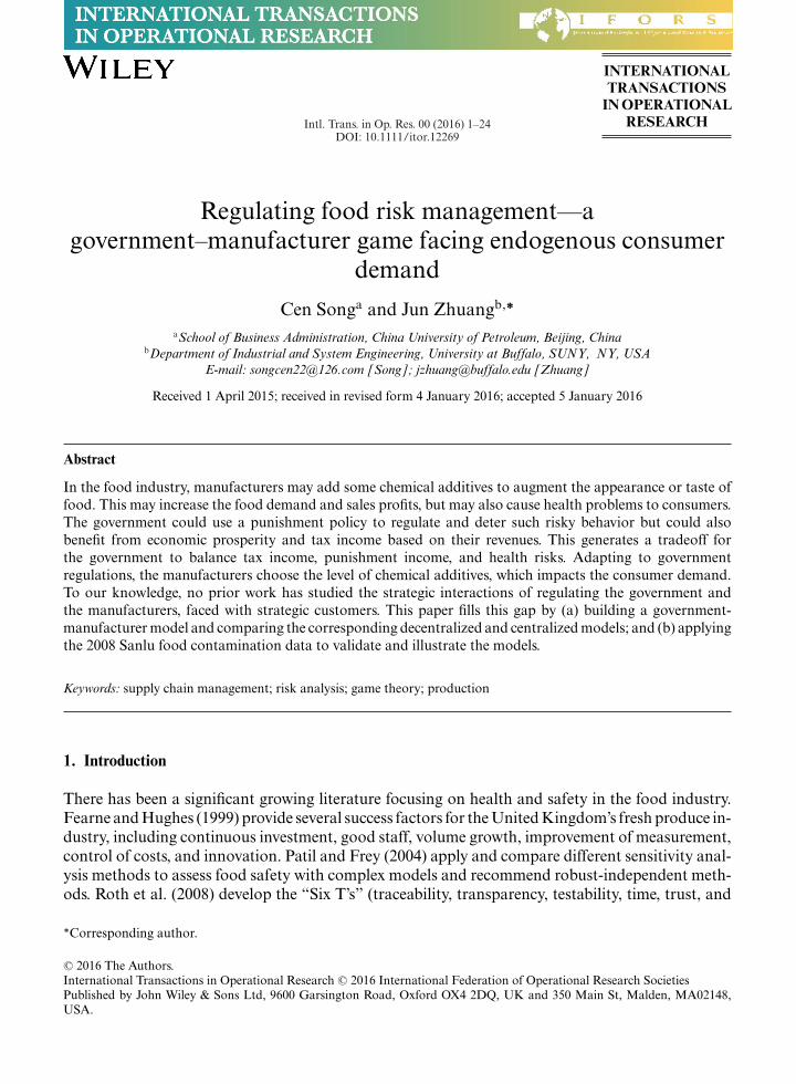
Figure 1 illustrates a general food industry process, where raw materials are initially raised byfarmers. The food is then transported by the distributors to the manufacturers for processing,and are eventually sold to and used by the consumers. This paper focuses on the risky behaviorof the manufacturers. During the process, chemical additives could be added by the farmers andmanufacturers. For example, the farmers could use chemicals to irrigate crops, or add hormonein the fodder to foster animal growth. The manufacturers could use whitening/antistaling/dyeingagents to better preserve food and enhance appearance. Farmers and manufacturers may overuse

C© 2016 The Authors.International Transactions in Operational Research C© 2016 International Federation of Operational Research Societies

C. Song and J. Zhuang / Intl. Trans. in Op. Res. 00 (2016) 1–24 3

Government

Farmers Manufacturers ConsumersRaise Sell

Inspect & Punish

Add Chemical Add Chemical

Fig. 1. Food industry with chemicals and regulating the government.

preservatives and antistaling agents to improve the product’s appearance or delay the decompositionprocess. Finally, the consumers could get sick from consuming the contaminated food. At eachstage of the food industry, the government could inspect (regulate) and punish (fine) each agent(e.g., farmers and manufacturers). Such government administrations include the US Food and DrugAdministration, European Food Safety Authority, and Chinese Institute of Food Safety Controland Inspection.

1.3. The manufacturer’s motivation for using chemicals

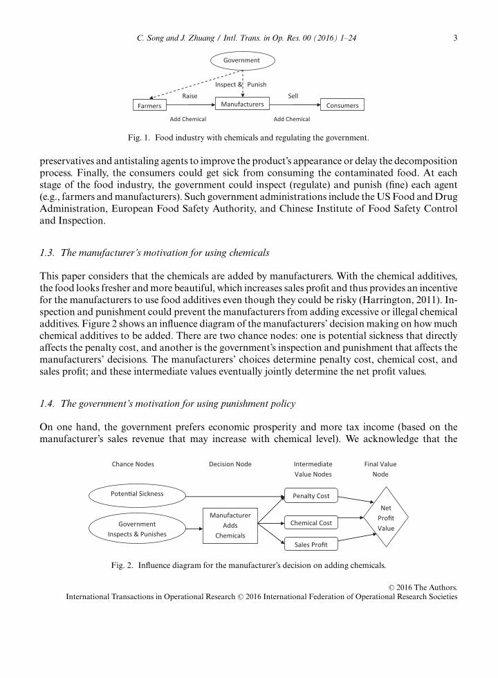
This paper considers that the chemicals are added by manufacturers. With the chemical additives,the food looks fresher and more beautiful, which increases sales profit and thus provides an incentivefor the manufacturers to use food additives even though they could be risky (Harrington, 2011). In-spection and punishment could prevent the manufacturers from adding excessive or illegal chemicaladditives. Figure 2 shows an influence diagram of the manufacturers’ decision making on how muchchemical additives to be added. There are two chance nodes: one is potential sickness that directlyaffects the penalty cost, and another is the government’s inspection and punishment that affects themanufacturers’ decisions. The manufacturers’ choices determine penalty cost, chemical cost, andsales profit; and these intermediate values eventually jointly determine the net profit values.

1.4. The government’s motivation for using punishment policy

On one hand, the government prefers economic prosperity and more tax income (based on themanufacturer’s sales revenue that may increase with chemical level). We acknowledge that the

GovernmentInspects & Punishes

ManufacturerAdds

Chemicals

Penalty Cost

Sales Profit

Chemical Cost

Net Profit Value

Chance Nodes Decision Node Intermediate Value Nodes

Final Value Node

Poten�al Sickness

Fig. 2. Influence diagram for the manufacturer’s decision on adding chemicals.



government may not directly maximize tax income; however, spending tax income is critical for thegovernment to improve the welfare of the country, including health improvement for its citizens. Onthe other hand, once consumers fall sick after consuming the contaminated food, the government isliable to treat and compensate those victims. This generates a tradeoff for the government to deter-mine how to punish the manufacturers’ risky behavior of adding chemicals. Once the governmentpunishment policy is set up, the manufacturers can observe it and respond by deciding the level ofchemical additives. The government would like to consider such potential response strategies of themanufacturers while deciding its own punishment policy.

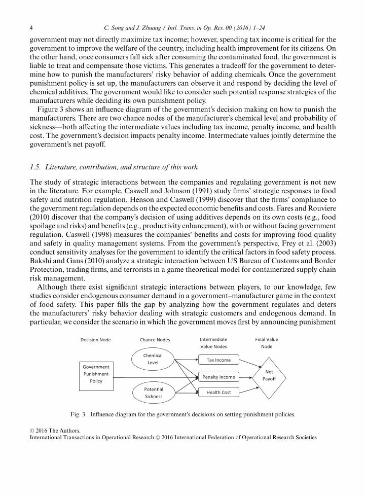
Figure 3 shows an influence diagram of the government’s decision making on how to punish themanufacturers. There are two chance nodes of the manufacturer’s chemical level and probability ofsickness—both affecting the intermediate values including tax income, penalty income, and healthcost. The government’s decision impacts penalty income. Intermediate values jointly determine thegovernment’s net payoff.

1.5. Literature, contribution, and structure of this work

The study of strategic interactions between the companies and regulating government is not newin the literature. For example, Caswell and Johnson (1991) study firms’ strategic responses to foodsafety and nutrition regulation. Henson and Caswell (1999) discover that the firms’ compliance tothe government regulation depends on the expected economic benefits and costs. Fares and Rouviere(2010) discover that the company’s decision of using additives depends on its own costs (e.g., foodspoilage and risks) and benefits (e.g., productivity enhancement), with or without facing governmentregulation. Caswell (1998) measures the companies’ benefits and costs for improving food qualityand safety in quality management systems. From the government’s perspective, Frey et al. (2003)conduct sensitivity analyses for the government to identify the critical factors in food safety process.Bakshi and Gans (2010) analyze a strategic interaction between US Bureau of Customs and BorderProtection, trading firms, and terrorists in a game theoretical model for containerized supply chainrisk management.

Although there exist significant strategic interactions between players, to our knowledge, fewstudies consider endogenous consumer demand in a government–manufacturer game in the contextof food safety. This paper fills the gap by analyzing how the government regulates and detersthe manufacturers’ risky behavior dealing with strategic customers and endogenous demand. Inparticular, we consider the scenario in which the government moves first by announcing punishment

Chance NodesDecision Node Intermediate Value Nodes

Final Value Node

GovernmentPunishment

Policy

Chemical Level Tax Income

Penalty IncomeNet

Payoff

Health CostPoten�alSickness

Fig. 3. Influence diagram for the government’s decisions on setting punishment policies.



policies, balancing punishment, tax income, and health risk. In the first scenario, the manufacturerobserves this punishment information and chooses the level of chemical additives, balancing theexpected punishment cost, sales revenue, and chemical cost.

The remainder of this paper is organized as follows. Section 2 describes optimization problems fora government–manufacturer model, provides the best responses for the manufacturer and optimalsolution for the government punishment policy with numerical illustration, and compares theequilibrium payoffs and strategies between the centralized and decentralized models. A decentralizedgovernment versus manufacturer (GvM) model and a centralized government/manufacturer (GM)model are introduced in Sections 2 and 2.5, respectively. Section 3 describes the Sanlu case andcompares the results of two models. Section 4 summarizes this paper and provides some futureresearch directions. Appendix provides the proofs for the propositions.

2. A GvM model

A decentralized GvM model is introduced in this section, where the government and manufacturerare modeled as two separate parties, and the strategic interaction between them is analyzed.

2.1. Notation, assumptions, and sequence of moves

Table 1 lists the notation that is used throughout this paper, including two decision variables (chem-ical level x and punishment level β), four functions (customer demand Q(x), sickness probabilityH (x), the government’s utility UG(x, β), and the manufacturer’s utility UM(x, β)), and nine pa-rameters (unit chemical cost pm, coefficient of health cost c, tax rate γ , basic demand Q0, slopefor customer demand q, unit food price P, slope for probability of sickness λ, the protein amountrequired in milk powder xp, and unit protein price pp).

Table 1Notation and explanation

Decision variables β ≥ 0 Level of punishment per sick customer set by the governmentx Level of chemical additives

Functions Q(x) ≥ 0 Consumer demandH (x) ∈ [0, 1] Probability of sicknessUG(x, β) The government’s utility functionUM (x, β) The manufacturer’s utility function

Parameters pm ≥ 0 Unit chemical cost[x−, x+] Chemical level lower bound x− and upper bound x+

c ≥ 0 Coefficient of health cost per number of sickness peopleγ ∈ [0, 1] Tax rateQ0 > 0 Baseline demand for Q(X )

q ≥ 0 Slope for Q(X )

P ≥ 0 Unit food priceλ ≥ 0 Slope for H (x)

xp ≥ 0 The amount of raw material required for productionpp ≥ 0 Unit raw material price



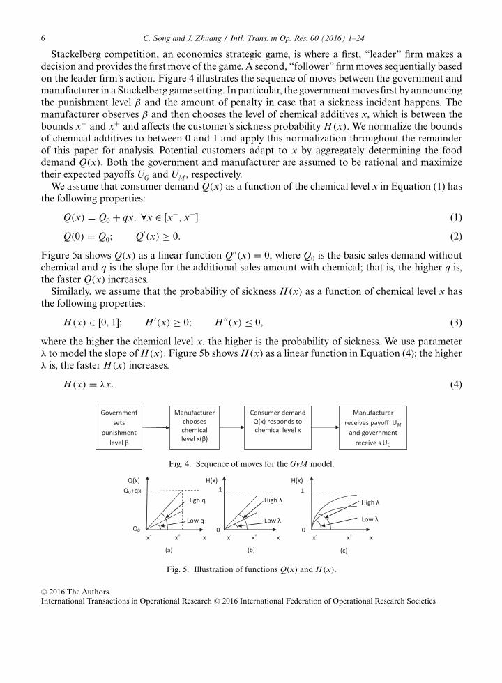
Stackelberg competition, an economics strategic game, is where a first, “leader” firm makes adecision and provides the first move of the game. A second, “follower” firm moves sequentially basedon the leader firm’s action. Figure 4 illustrates the sequence of moves between the government andmanufacturer in a Stackelberg game setting. In particular, the government moves first by announcingthe punishment level β and the amount of penalty in case that a sickness incident happens. Themanufacturer observes β and then chooses the level of chemical additives x, which is between thebounds x− and x+ and affects the customer’s sickness probability H (x). We normalize the boundsof chemical additives to between 0 and 1 and apply this normalization throughout the remainderof this paper for analysis. Potential customers adapt to x by aggregately determining the fooddemand Q(x). Both the government and manufacturer are assumed to be rational and maximizetheir expected payoffs UG and UM, respectively.

We assume that consumer demand Q(x) as a function of the chemical level x in Equation (1) hasthe following properties:

Q(x) = Q0 + qx, ∀x ∈ [x−, x+] (1)

Q(0) = Q0; Q′(x) ≥ 0. (2)

Figure 5a shows Q(x) as a linear function Q′′(x) = 0, where Q0 is the basic sales demand withoutchemical and q is the slope for the additional sales amount with chemical; that is, the higher q is,the faster Q(x) increases.

Similarly, we assume that the probability of sickness H (x) as a function of chemical level x hasthe following properties:

H (x) ∈ [0, 1]; H ′(x) ≥ 0; H ′′(x) ≤ 0, (3)

where the higher the chemical level x, the higher is the probability of sickness. We use parameterλ to model the slope of H (x). Figure 5b shows H (x) as a linear function in Equation (4); the higherλ is, the faster H (x) increases.

H (x) = λx. (4)

Fig. 4. Sequence of moves for the GvM model.

1

(a) (b) (c)

High λ

Low λLow q

High q

Q(x)

High λ

Low λ

H(x) H(x)Q0+qx

Q0 0 0

1

x- x- x-x+ x+ xx x+ x

Fig. 5. Illustration of functions Q(x) and H (x).



2.2. The manufacturer’s and government’s optimization problems and definition of equilibrium

In this section, we assume that the chemical x provides productivity enhancement, where a manu-facturer can substitute chemical x with lower cost pm for part of the original production material xpwith higher cost pp. Therefore, the chemical is the substitute for production raw material, where xphas negative relationship with x. We assume that the manufacturer chooses the chemical additiveslevel x to maximize his expected payoff shown in Equation (5) that consists of four items: (a) totalsales revenue PQ(x), (b) total production cost including chemical cost pmxQx and production costppxpQx, (c) expected punishment cost βQ(x)H (x), and (d) tax cost γ PQ(x).

maxx∈[x−,x+]

UM(x, β) = PQ(x)︸︷︷︸Sales Revenue

− pmxQ(x)︸︷︷︸Chemical Cost

− ppxpQ(x)︸︷︷︸Production Cost

− βQ(x)H (x)︸︷︷︸Punishment Cost

− γ PQ(x)︸︷︷︸Tax Cost

. (5)

One of the government’s roles is to supervise and regulate the firms/manufacturers in case of anyrisky behavior in food industry by setting punishment policy for the sake of public health. Anotherrole of the government is, in order to maintain a stable and healthy economic growth and employmentrate, the government will not put too much economic burden to discourage firms’/manufacturers’development. On the other hand, tax income through the firms’/manufacturers’ sales revenueand punishment income are the fiscal income used for fiscal expenditure such as social welfareexpenditure–public medical service. Therefore, based on the tradeoff of the government, we assumethat the government chooses the punishment level β to maximize his expected payoff shown inEquation (6) that consists of three items: (a) expected health cost (public health expenditure)cQ(x)H (x), (b) punishment income βQ(x)H (x), and (c) tax income γ PQ(x).

maxβ≥0

UG(x, β) = − cQ(x)H (x)︸︷︷︸Health Cost

+ βQ(x)H (x)︸︷︷︸Punishment Income

+ γ PQ(x)︸︷︷︸Tax Income

. (6)

Definition 1. We call a strategy pair (x∗, β∗) a subgame-perfect Nash equilibrium, or “equilibrium”for the GvM model, if and only if both Equations (7) and (8) are satisfied:

x∗ = x̂(β∗) (7)

β∗ = argmaxβ≥0

UG(x̂(β), β), (8)

where the manufacturer’s best response is defined to be

x̂(β) ≡ argmaxx∈[x−,x+]

UM(x, β), ∀β ≥ 0. (9)

2.3. Solution

In this section, we analyze the manufacturer’s best response and the government’s optimal regulatingpolicy.



Proposition 1. Under some technical second-order condition Q(x)H ′′(x) + 2Q′(x)H ′(x) ≥ 0, the so-lution to the manufacturer’s optimization problem (9) is given by

x̂(β) =

⎧⎪⎪⎪⎪⎪⎪⎪⎪⎪⎨⎪⎪⎪⎪⎪⎪⎪⎪⎪⎩

x− if∂UM(x, β)

∂x

∣∣∣∣x=x−

≤ 0

x+ if∂UM(x, β)

∂x

∣∣∣∣x=x+

≥ 0

{x :

∂UM(x, β)

∂x= 0

}if

∂UM(x, β)

∂x

∣∣∣∣x=x−

> 0 >∂UM(x, β)

∂x

∣∣∣∣x=x+

,

(10)

where ∂UM (x,β)

∂x = (1 − γ )PQ′(x) − βH ′(x)Q(x) − βH (x)Q′(x) − pmxQ′x − pmQ(x) − ppxpQ′(x)

is the marginal payoff for the manufacturer. We also have dx̂dβ

≤ 0.

Remark. Proposition 1 shows that there exist three types of optimal chemical levels: (a) when themarginal payoff is negative at x = x−, the manufacturer uses a lower chemical bound x−; (b) themanufacturer sets the chemical additives at an intermediate level, such that the marginal benefitequals the marginal cost; and (c) when the marginal payoff is positive at x = x+, the manufacturertakes the highest possible chemical level x+. In addition, the manufacturer’s chemical level decreases(weakly) with the government punishment level.

The government’s optimal punishment policy is analyzed in Proposition 2.

Proposition 2. The optimal strategy for the government is as follows:

β =

⎧⎪⎪⎪⎨⎪⎪⎪⎩

0 ifdUG(x̂(β), β)

dβ

∣∣∣∣β=0

< 0

{β :

dUG(x̂(β), β)

dβ= 0

}if

dUG(x̂(β), β)

dβ

∣∣∣∣β=0

≥ 0,

(11)

where dUG(x̂(β),β)

dβ= ∂UG

∂β+ ∂UG

∂xdx̂(β)

dβis the total marginal payoff for the government.

Remark. Proposition 2 indicates that when the total marginal payoff for the government dUG(x̂(β),β)

dβ

is positive at β = 0, the optimal punishment is such that the marginal payoff equals the marginalcost, otherwise the optimal punishment is 0.

2.4. Solution and illustration when H (x) = λx and Q(x) = Q0 + qx

This section uses specific linear Q(x) and H (x) functions introduced in Equations (1) and (4) forstudying and illustrating equilibrium solutions.



0

0.5

1

0

0.5

10

1

2

3

4

xβ

UM

11.21.41.6

1.8

1.8

1.8

1.8

22

2 2

2

2.2

2.2

2.2

2.4

2.4 2.4

2.6

2.6

2.8

2.83

3.2

3.4

x: Chemical Amount

β: P

unis

hmen

t Cos

t Coe

ffici

ent

0 0.2 0.4 0.6 0.8 10

0.2

0.4

0.6

0.8

1

(a) Manufacturer Payoff (3D) (b) Manufacturer Payoff (Contour)

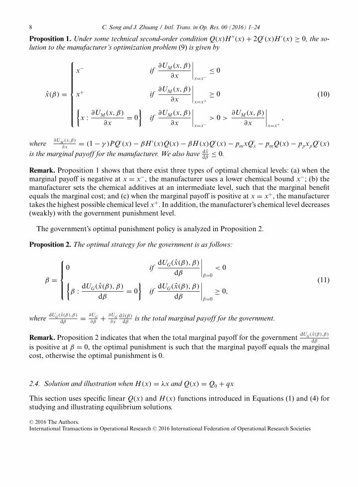
Fig. 6. The manufacturer’s payoffs as functions of strategies x and β, using baseline values γ = 0.1, P = 2, Q0 = 1,q = 2, c = 1, pm = 0.5, λ = 0.1, xp = 0.1, pp = 0.6, x− = 0, and x+ = 1.

2.4.1. The manufacturer’s best responseInserting Equations (1) and (4) into Equation (5), the manufacturer’s optimization problembecomes

maxx∈[x−,x+]

UM(x, β) = (P(1 − γ ) − ppxp)Q0 + ((1 − γ )Pq − pmQ0 − βλQ0 − ppxpq)x

−(βλ + pm)qx2.(12)

Figure 6 illustrates how the combination of chemical and punishment levels affect the manufacturers’payoff, using the baseline values γ = 0.1, P = 2, Q0 = 1, q = 2, c = 1, pm = 0.5, λ = 0.1, xp = 0.1,pp = 0.6, x− = 0, and x+ = 1. We observe that the manufacturer’s payoff increases in chemicalamount x when punishment level β is low but decreases in x when β is high. The manufacturer’spayoff also decreases in punishment level β, which means that the punishment level should not betoo high in order to maintain the manufacturer’s payoff.

Applying Proposition 1, with the bounds x− = 0 and x+ = 1, the solution to the manufacturer’soptimization problem (12) becomes

x̂(β) =

⎧⎪⎪⎪⎨⎪⎪⎪⎩

0 if β ≥ βA

Pq − γ Pq − pmQ0 − βλQ0 − ppxpq

2βλq + 2pmqif βC < β < βA

1 if β ≤ βC,

(13)

where the two thresholds for β are defined as βA ≡ Pq−γ Pq−pmQ0−ppxpqλQ0

and βC ≡Pq−γ Pq−pmQ0−ppxpq−2pmq

λQ0+2λq , and we have βA ≥ βC ≥ 0 if Pq − γ Pq − pmQ0 − ppxpq ≥ 0 or βA ≤ βC ≤ 0

if Pq − γ Pq − pmQ0 − ppxpq − 2pmq ≤ 0. The second-order condition holds since ∂2UM (x,β)

∂x2 =−2βλq − 2pmq ≤ 0. We also verify that the manufacturer’s optimal chemical amount decreases



in punishment because dx̂dβ

= −λQ0(βλq+pmq)+λq(Pq−γ Pq−pmQ0−βλQ0−ppxpq)

2(λcq+pmq)2 ≤ 0, when βC < β < βA anddx̂dβ

= 0 otherwise.This paper only concerns a company’s risky behavior for short-term benefit in a nontransparent

supply chain. With the increasing transparency in the food industry and the consumers’ food safetyconcerns, the demand could decrease if the chemical level increases, which means q < 0. In thiscase, based on Equation (13), we have βA < 0. Since the punishment level β ≥ 0 > βA, we alwayshave x̂ = 0. This indicates that in the long run, as the consumer’s health-related concern rises andthe transparency in food industry increases, the company would not add chemicals with or withoutpunishment policy.

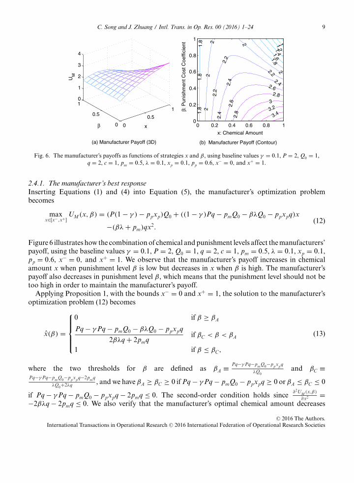
Figure 7 shows how the government’s punishment β affects the value of chemical level x, usingthe same baseline values as in Fig. 6. In particular, when the food price P is low (P = 0.3), Fig.7a shows that the optimal chemical amount x∗ = 0 for all punishment levels β, where βA = −0.8and βC = −3.92. When the food price is intermediate (P = 1), Fig. 7b shows that as β increases,x∗ decreases to zero at the point β = βA = 11.8 (i.e., deterred by punishment), where βC = −1.4.When the food price is P = 2, Fig. 7c shows that as β increases, x∗ first remains 1 until the pointβ = βC = 2.2, and then decreases to zero at the point β = βA = 29.8 (i.e., deterred by punishment).Comparing Fig. 7a–c, we observe that there is no need to set high punishment levels to preventrisky behavior when the food price is low but when the food price is high, a higher punishment levelis needed for deterrence.

2.4.2. The government’s optimal strategiesInserting Equations (1) and (4) into Equation (6), the government’s optimization problem becomes

maxβ≥0

UG(x̂(β), β) = γ PQ0 + (γ Pq + λβQ0 − cλQ0)x̂(β) + (β − c)qλx̂2(β). (14)

βA=−0.8

βC

=−3.92

−2 −1 0 10

0.10.20.30.40.50.60.70.80.9

1

(a) P=0.3

x*

0 5 10 150

0.1

0.2

0.3

0.4

0.5

0.6

0.7

βA=11.8

βC

=−1.4

β

x*

(b) P=1

0 20 400

0.2

0.4

0.6

0.8

1

βA=29.8

βC

=2.2

β

x*

(c) P=2

β

Fig. 7. Illustration of the manufacturer’s best responses as functions of the government’s punishment strategies β usingbaseline values γ = 0.1, Q0 = 1, q = 2, c = 1, pm = 0.5, λ = 0.1, xp = 0.1, and pp = 0.6.



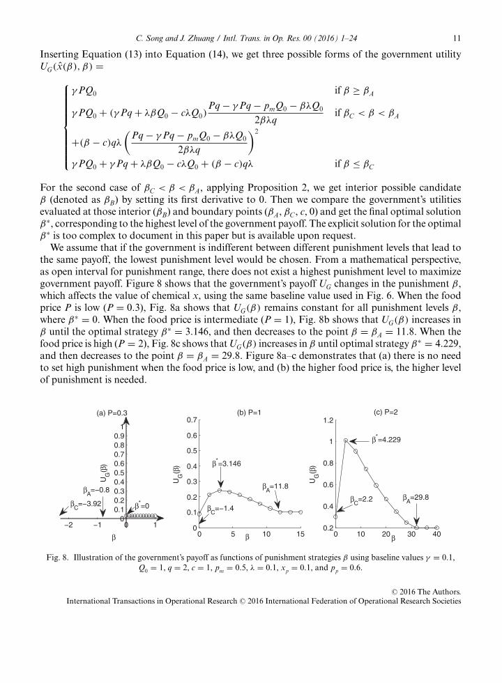
Inserting Equation (13) into Equation (14), we get three possible forms of the government utilityUG(x̂(β), β) =

⎧⎪⎪⎪⎪⎪⎪⎪⎪⎨⎪⎪⎪⎪⎪⎪⎪⎪⎩

γ PQ0 if β ≥ βA

γ PQ0 + (γ Pq + λβQ0 − cλQ0)Pq − γ Pq − pmQ0 − βλQ0

2βλqif βC < β < βA

+(β − c)qλ

(Pq − γ Pq − pmQ0 − βλQ0

2βλq

)2

γ PQ0 + γ Pq + λβQ0 − cλQ0 + (β − c)qλ if β ≤ βC

For the second case of βC < β < βA, applying Proposition 2, we get interior possible candidateβ (denoted as βB) by setting its first derivative to 0. Then we compare the government’s utilitiesevaluated at those interior (βB) and boundary points (βA, βC, c, 0) and get the final optimal solutionβ∗, corresponding to the highest level of the government payoff. The explicit solution for the optimalβ∗ is too complex to document in this paper but is available upon request.

We assume that if the government is indifferent between different punishment levels that lead tothe same payoff, the lowest punishment level would be chosen. From a mathematical perspective,as open interval for punishment range, there does not exist a highest punishment level to maximizegovernment payoff. Figure 8 shows that the government’s payoff UG changes in the punishment β,which affects the value of chemical x, using the same baseline value used in Fig. 6. When the foodprice P is low (P = 0.3), Fig. 8a shows that UG(β) remains constant for all punishment levels β,where β∗ = 0. When the food price is intermediate (P = 1), Fig. 8b shows that UG(β) increases inβ until the optimal strategy β∗ = 3.146, and then decreases to the point β = βA = 11.8. When thefood price is high (P = 2), Fig. 8c shows that UG(β) increases in β until optimal strategy β∗ = 4.229,and then decreases to the point β = βA = 29.8. Figure 8a–c demonstrates that (a) there is no needto set high punishment when the food price is low, and (b) the higher food price is, the higher levelof punishment is needed.

βA=−0.8

βC

=−3.92 β*=0

−2 −1 0 10

0.10.20.30.40.50.60.70.80.9

1

β

UG

(β)

(a) P=0.3

0 5 10 150

0.1

0.2

0.3

0.4

0.5

0.6

0.7

βA=11.8

βC

=−1.4

β*=3.146

β

UG

(β)

(b) P=1

0 10 20 30 400.2

0.4

0.6

0.8

1

1.2

βA=29.8β

C=2.2

β*=4.229

β

UG

(β)

(c) P=2

β

Fig. 8. Illustration of the government’s payoff as functions of punishment strategies β using baseline values γ = 0.1,Q0 = 1, q = 2, c = 1, pm = 0.5, λ = 0.1, xp = 0.1, and pp = 0.6.



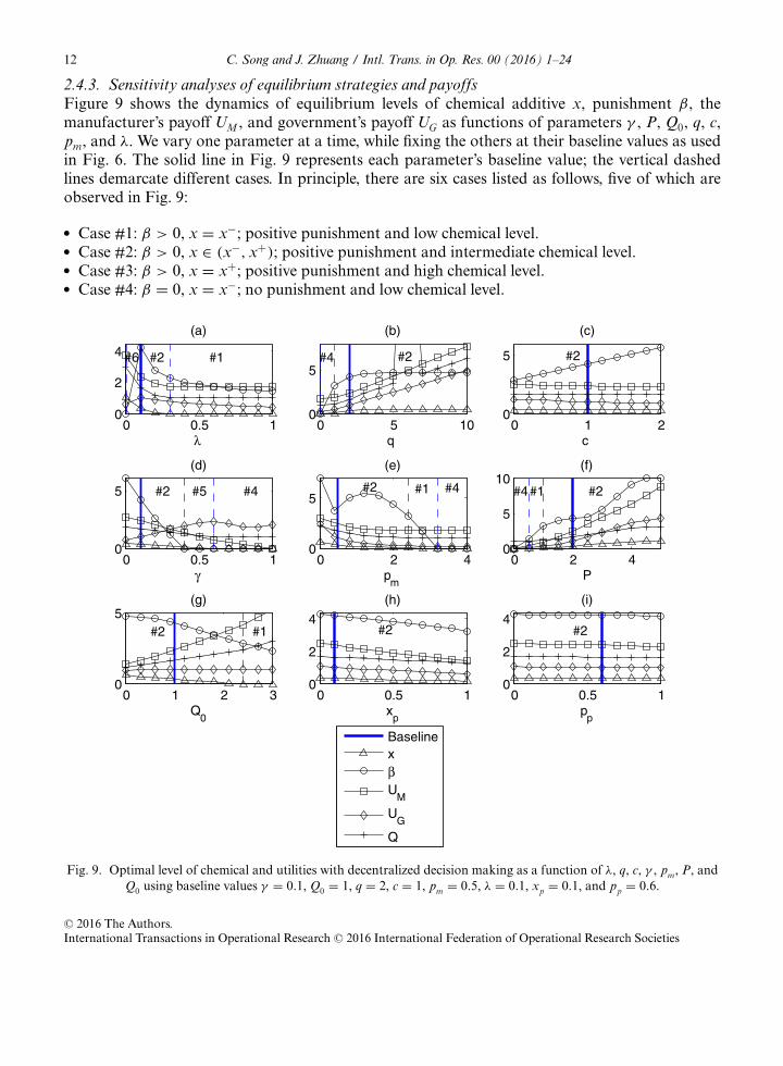
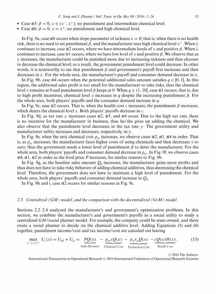
2.4.3. Sensitivity analyses of equilibrium strategies and payoffsFigure 9 shows the dynamics of equilibrium levels of chemical additive x, punishment β, themanufacturer’s payoff UM, and government’s payoff UG as functions of parameters γ , P, Q0, q, c,pm, and λ. We vary one parameter at a time, while fixing the others at their baseline values as usedin Fig. 6. The solid line in Fig. 9 represents each parameter’s baseline value; the vertical dashedlines demarcate different cases. In principle, there are six cases listed as follows, five of which areobserved in Fig. 9:

� Case #1: β > 0, x = x−; positive punishment and low chemical level.� Case #2: β > 0, x ∈ (x−, x+); positive punishment and intermediate chemical level.� Case #3: β > 0, x = x+; positive punishment and high chemical level.� Case #4: β = 0, x = x−; no punishment and low chemical level.

0 0.5 10

2

4 #6 #2 #1

λ

(a)

BaselinexβU

M

UG

Q

0 5 100

5#4 #2

q

(b)

0 1 20

5 #2

c

(c)

0 0.5 10

5 #2 #5 #4

γ

(d)

0 2 40

5#2 #1 #4

pm

(e)

0 2 40

5

10#4#1 #2

P

(f)

0 1 2 30

5#2 #1

Q0

(g)

0 0.5 10

2

4#2

xp

(h)

0 0.5 10

2

4#2

pp

(i)

Fig. 9. Optimal level of chemical and utilities with decentralized decision making as a function of λ, q, c, γ , pm, P, andQ0 using baseline values γ = 0.1, Q0 = 1, q = 2, c = 1, pm = 0.5, λ = 0.1, xp = 0.1, and pp = 0.6.



� Case #5: β = 0, x ∈ (x−, x+); no punishment and intermediate chemical level.� Case #6: β = 0, x = x+; no punishment and high chemical level.

In Fig. 9a, case #6 occurs when slope parameter of sickness λ = 0; that is, when there is no healthrisk, there is no need to set punishment β, and the manufacturer uses high chemical level x+. When λ

continues to increase, case #2 occurs, where we have intermediate levels of x and positive β. When λ

continues to increase, case #1 occurs, where we have low level of x and positive β. We observe that asλ increases, the manufacturer could be punished more due to increasing sickness and thus choosesto decrease the chemical level; as a result, the government punishment level could decrease. In otherwords, it is noteworthy to see that punishment β and government’s payoff first increases and thendecreases in λ. For the whole area, the manufacturer’s payoff and consumer demand decrease in λ.

In Fig. 9b, case #4 occurs when the potential additional sales amount satisfies q ∈ [0, 1]. In thisregion, the additional sales profit is too small for the manufacturer to take risks, thus the chemicallevel x remains at 0 and punishment level β keeps at 0. When q ∈ (1, 10], case #1 occurs; that is, dueto high profit incentives, chemical level x increases in q despite the increasing punishment β. Forthe whole area, both players’ payoffs and the consumer demand increase in q.

In Fig. 9c, case #2 occurs. That is, when the health cost c increases, the punishment β increases,which deters the chemical level x. Both players’ payoffs decrease in c.

In Fig. 9d, as tax rate γ increases cases #2, #5, and #4 occur. Due to the high tax rate, thereis no incentive for the manufacturer in business, thus he/she gives up adding the chemical. Wealso observe that the punishment level decreases in the tax rate γ . The government utility andmanufacturer utility increases and decreases, respectively, in γ .

In Fig. 9e, when the unit chemical cost pm increases, we observe cases #2, #1, #4 in order. Thatis, as pm increases, the manufacturer faces higher costs of using chemicals and then decreases x tozero; thus the government needs a lower level of punishment β to deter the manufacturer. For thewhole area, both players’ payoffs and consumer demand decrease in pm. In Fig. 9f, we observe cases#4, #1, #2 in order as the food price P increases, for similar reasons to Fig. 9b.

In Fig. 9g, as the baseline sales amount Q0 increases, the manufacturer gains more profits andthus does not have to take risky behavior of adding chemical additives, thus decreasing the chemicallevel. Therefore, the government does not have to maintain a high level of punishment. For thewhole area, both players’ payoffs and consumer demand increase in Q0.

In Fig. 9h and i, case #2 occurs for similar reasons in Fig. 9c.

2.5. Centralized (GM) model, and the comparison with the decentralized (GvM) model

Sections 2.2–2.4 analyzed the manufacturer’s and government’s optimization problems. In thissection, we combine the manufacturer’s and government’s payoffs as a social utility to study acentralized GM/social planner model. For example, the company could be state-owned, and thereexists a social planner to decide on the chemical additive level. Adding Equations (5) and (6)together, punishment income/cost and tax income/cost are canceled out leaving

maxx−≤x≤x+

Uc(x) = UM + UG = PQ(x)︸︷︷︸Sales Revenue

− pmxQ(x)︸︷︷︸Chemical Cost

− ppxpQ(x)︸︷︷︸Production Cost

− cQ(x)H (x)︸︷︷︸Health Cost

. (15)



Note that in this societal problem (15), the government punishment level no longer matters and weonly have one decision variable, the chemical level x.

Using function forms specified in Equations (1) and (4), Equation (15) becomes

Uc(x) = (P − ppxp)Q0 + (Pq − pmQ0 − cλQ0 − ppxpq)x − (λcq + pmq)x2. (16)

Solving Equation (16), the optimal chemical level is attained when x− = 0 and x+ = 1.

xc∗ =

⎧⎪⎪⎪⎪⎪⎪⎪⎪⎨⎪⎪⎪⎪⎪⎪⎪⎪⎩

0 ifPq − pmQ0 − cλQ0 − ppxpq

2qcλ + 2pmq≤ 0

Pq − pmQ0 − cλQ0 − ppxpq

2qcλ + 2pmqif

Pq − pmQ0 − cλQ0 − ppxpq

2qcλ + 2pmq∈ (0, 1)

1 ifPq − pmQ0 − cλQ0 − ppxpq

2qcλ + 2pmq≥ 1.

(17)

Based on Equations (10) and (17), we have

xc∗ − x̂ = γ pmP − (1 − γ )λcP − ppxpλc + βλ(P − ppxp)

2(βλ + pm)(λc + pm)if x̂, xc

∗ ∈ (0, 1). (18)

As in Proof of Proposition 2, we have xc∗ ≥ x̂ when β ≥ (1−γ )λcP−γ pmP−ppxpcγ

λP−λppxp, which means that

sufficiently high punishment could lead to less risky behavior under decentralized policy.Figures 10 and 11 compare the equilibrium chemical amounts and societal utilities between the

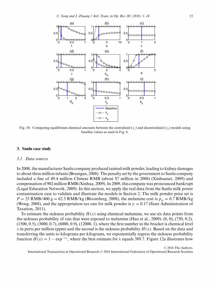
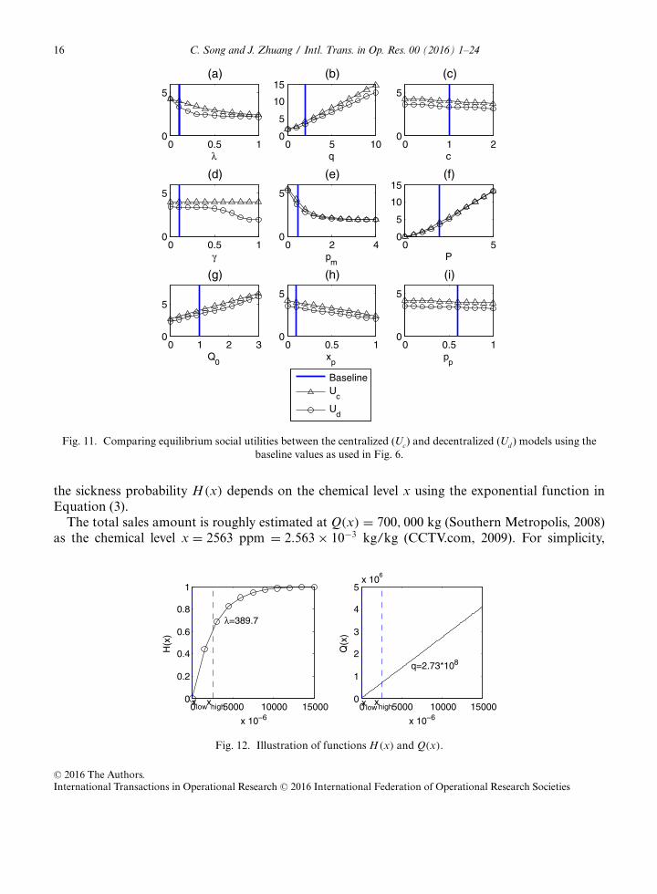
centralized (xc and Uc, respectively) and decentralized (xd and Ud , respectively) models, using thesame baseline values as in Fig. 6. In Fig. 10, it is noteworthy that xd is smaller than (or equals to)xc, especially when the potential additional sales amount q and the unit chemical cost pm (Fig. 10band e) are low, or when the slope parameter of sickness λ and food price P (Fig. 10a and f) are atintermediate levels, or when the tax rate γ , baseline sales amount Q0, required protein amount xp,and unit protein price pp (Fig. 10d and g–i) are high. In Fig. 11, we see that the social utility from thedecentralized model Ud is always smaller than (or equals to) the society utility from the centralizedmodel Uc, and the difference is significant especially when the unit chemical cost pm (Fig. 11e) islow, or when the slope parameter of sickness λ and food price P (Fig. 11a and f) are at intermediatelevels, or when the potential additional sales amount q and tax rate γ (Fig. 11b and d) are high.

Equation (19) summarizes the breakdown of the societal utility changes from the decentralized tocentralized models, where the sales revenue increases but the chemical cost and health cost decrease.Although the centralized model leads to higher societal utility, it also leads to higher chemical leveland lower production cost.

Uc︸︷︷︸Total Payoff↗

= PQ(x)︸︷︷︸Sales Rvenue↗

− pmxQ(x)︸︷︷︸Chemical Cost↗

− ppxpQ(x)︸︷︷︸Production Cost↙

− cQ(x)H (x)︸︷︷︸Health Cost↗

. (19)



0 0.5 10

0.5

1

λ

(a)

0 5 100

0.5

1

q

(b)

0 1 20

0.5

1

c

(c)

0 0.5 10

0.5

1

γ

(d)

Baselinex

c

xd

0 2 40

0.5

1

pm

(e)

0 50

0.5

1

P

(f)

0 1 2 30

0.5

1

Q0

(g)

0 0.5 10

0.5

1

xp

(h)

0 0.5 10

0.5

1

pp

(i)

Fig. 10. Comparing equilibrium chemical amounts between the centralized (xc) and decentralized (xd ) models usingbaseline values as used in Fig. 6.

3. Sanlu case study

3.1. Data sources

In 2008, the manufacturer Sanlu company produced tainted milk powder, leading to kidney damagesto about three million infants (Branigan, 2008). The penalty set by the government to Sanlu companyincluded a fine of 49.4 million Chinese RMB (about $7 million in 2008) (Xinhuanet, 2009) andcompensation of 902 million RMB (Xinhua, 2009). In 2009, this company was pronounced bankrupt(Legal Education Network, 2009). In this section, we apply the real data from the Sanlu milk powercontamination case to validate and illustrate the models in Section 2. The milk powder price set isP = 25 RMB/400 g = 62.5 RMB/kg (Bloomberg, 2008), the melamine cost is pm = 0.7 RMB/kg(Wong, 2008), and the appropriation tax rate for milk powder is γ = 0.17 (State Administration ofTaxation, 2011).

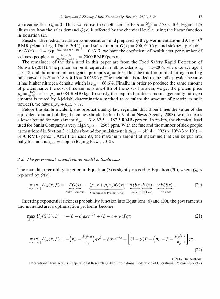
To estimate the sickness probability H (x) using chemical melamine, we use six data points fromthe sickness probability of rats that were exposed to melamine (Hau et al., 2009): (0, 0), (750, 0.2),(1500, 0.5), (3000, 0.7), (6000, 0.9), (12000, 1), where the first number in the bracket is chemical levelx in parts per million (ppm) and the second is the sickness probability H (x). Based on the data andtransferring the units to kilograms per kilograms, we exponentially regress the sickness probabilityfunction H (x) = 1 − exp−λx, where the best estimate for λ equals 389.7. Figure 12a illustrates how



0 0.5 10

5

λ

(a)

0 5 100

5

10

15

q

(b)

0 1 20

5

c

(c)

0 0.5 10

5

γ

(d)

BaselineU

c

Ud

0 2 40

5

pm

(e)

0 50

5

10

15

P

(f)

0 1 2 30

5

Q0

(g)

0 0.5 10

5

xp

(h)

0 0.5 10

5

pp

(i)

Fig. 11. Comparing equilibrium social utilities between the centralized (Uc) and decentralized (Ud ) models using thebaseline values as used in Fig. 6.

the sickness probability H (x) depends on the chemical level x using the exponential function inEquation (3).

The total sales amount is roughly estimated at Q(x) = 700, 000 kg (Southern Metropolis, 2008)as the chemical level x = 2563 ppm = 2.563 × 10−3 kg/kg (CCTV.com, 2009). For simplicity,

0 5000 10000 150000

0.2

0.4

0.6

0.8

1

xlowxhigh

x 10−6

H(x

)

λ=389.7

0 5000 10000 150000

1

2

3

4

5x 10

6

xlowxhigh

q=2.73*108

x 10−6

Q(x

)

Fig. 12. Illustration of functions H (x) and Q(x).



we assume that Q0 = 0. Thus, we derive the coefficient to be q = Q(x)

x = 2.73 × 108. Figure 12billustrates how the sales demand Q(x) is affected by the chemical level x using the linear functionin Equation (2).

Based on the medical treatment compensation fund prepared by the government, around 9.1 × 108

RMB (Henan Legal Daily, 2011), total sales amount Q(x) = 700, 000 kg, and sickness probabil-ity H (x) = 1 − exp−389.7×2.563×10−3 = 0.6317, we have the coefficient of health cost per number ofsickness people c = 9.1×108

700,000×0.6317 = 2000 RMB/person.The remainder of the data used in this paper are from the Food Safety Rapid Detection of

Network (2011): The protein amount required in milk powder is xp = 15–20%, where we average itas 0.18, and the amount of nitrogen in protein is np = 16%, thus the total amount of nitrogen in 1 kgmilk powder is N = 0.18 × 0.16 = 0.0288 kg. The melamine is added to the milk powder becauseit has higher nitrogen density, which is nm = 66.6%. Finally, in order to produce the same amountof protein, since the cost of melamine is one-fifth of the cost of protein, we get the protein pricepp = 16%

66.6% × 5 × pm = 0.84 RMB/kg. To satisfy the required protein amount (generally nitrogenamount is tested by Kjeldahl determination method to calculate the amount of protein in milkpowder), we have npxp + nmx ≥ N.

Before the Sanlu incident, the product quality law regulates that three times the value of theequivalent amount of illegal incomes should be fined (Xinhua News Agency, 2008), which meansa lower bound for punishment βlow = 3 × 62.5 = 187.5 RMB/person. In reality, the chemical levelused for Sanlu Company is very high xhigh = 2563 ppm. With the fine and the number of sick peopleas mentioned in Section 3, a higher bound for punishment is βhigh = (49.4 + 902) × 106/(3 × 106) =3170 RMB/person. After the incidents, the maximum amount of melamine that can be put intobaby formula is xlow = 1 ppm (Beijing News, 2012).

3.2. The government–manufacturer model in Sanlu case

The manufacturer utility function in Equation (5) is slightly revised to Equation (20), where Q0 isreplaced by Q(x).

maxx∈[x−,x+]

UM(x, β) = PQ(x)︸︷︷︸Sales Revenue

− (pmx + ppxp)Q(x)︸︷︷︸Chemical & Protein Cost

− βQ(x)H (x)︸︷︷︸Punishment Cost

− γ PQ(x)︸︷︷︸Tax Cost

. (20)

Inserting exponential sickness probability function into Equations (6) and (20), the government’sand manufacturer’s optimization problems become

maxβ≥0

UG(x̂(β), β) = −(β − c)qxe−λx + (β − c + γ )Pqx (21)

maxx∈[x−,x+]

UM(x, β) = −(

pm − ppnm

np

)qx2 + βqxe−λx +

[(1 − γ )P −

(pm − β − ppN

np

)]qx.

(22)



The total utility in Equation (15) for the centralized case becomes the summation of Equations(21) and (22) given by

maxx−≤x≤x+

Uc(x) = −q(

pm − ppnm

np

)x2 + cqxe−λx + q

(P − ppN

np− c

)x. (23)

3.3. Illustration of the manufacturer’s best response based on punishment

Figure 13 illustrates how the government punishment β affects the chemical level x and the gov-ernment’s and manufacturer’s utilities UG and UM with real data. In Fig. 13a, the point (βlow, xhigh)

corresponds to Sanlu Company’s behavior, and the point (βhigh, xlow) corresponds to the new milkpowder regulation. Corresponding these two points (βlow, xhigh) and (βhigh, xlow), we use regressionmodel to estimate two new slopes of sickness probability λ = 60.3 and λ = 7820, respectively.Recall that we have λ = 389.7 corresponding to the data from Hau et al. (2009) as mentioned in

0 2000 4000 6000 8000 100000

5

10

xhighSanlu

xlowNew

βlowβhigh

λ=7820

λ=389.7

β

log(

x* +1)

106

(a) x*(β)

λ=60.3

0 2000 4000 6000 8000 100000

20

40

60

βlow βhigh

Government Utility UG

Manufacturer Utility UM

β

UG

, UM

104

(b) UG(β, x*(β)), UM* (β) when λ=389.7

0 2000 4000 6000 8000 100000

20

40

60

βlow βhigh

Health Cost

Punishment Income

Tax Income

β

UG

104

(c) Parts of Government Utility when λ=389.7

Fig. 13. Illustration of the manufacturer’s best response based on punishment using Sanlu real data.



Section 3.1. Figure 13a shows that as the punishment β increases, the chemical level x decreases. Inaddition, as the sickness probability slope λ decreases, the chemical level x increases, which meansthat the manufacturer would take riskier behavior. Figure 13b demonstrates that as punishment β

increases, the government’s utility UG increases and manufacturer’s utility UM decreases. Figure 13cfurther details how the government utility is affected by β in health cost, punishment income, andtax income, where all these decrease in β. The health cost decreases more than the others, whichreflects that now the manufacturer is deterred from using chemicals by a high punishment level.

3.4. Sensitivity analysis of equilibrium strategies for Sanlu case study

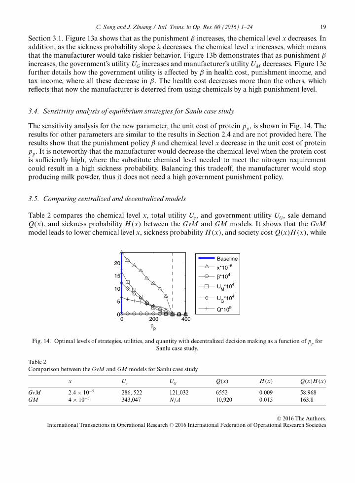
The sensitivity analysis for the new parameter, the unit cost of protein pp, is shown in Fig. 14. Theresults for other parameters are similar to the results in Section 2.4 and are not provided here. Theresults show that the punishment policy β and chemical level x decrease in the unit cost of proteinpp. It is noteworthy that the manufacturer would decrease the chemical level when the protein costis sufficiently high, where the substitute chemical level needed to meet the nitrogen requirementcould result in a high sickness probability. Balancing this tradeoff, the manufacturer would stopproducing milk powder, thus it does not need a high government punishment policy.

3.5. Comparing centralized and decentralized models

Table 2 compares the chemical level x, total utility Uc, and government utility UG, sale demandQ(x), and sickness probability H (x) between the GvM and GM models. It shows that the GvMmodel leads to lower chemical level x, sickness probability H (x), and society cost Q(x)H (x), while

0 200 4000

5

10

15

20

pp

Baseline

x*10−6

β*104

UM*104

UG*104

Q*109

Fig. 14. Optimal levels of strategies, utilities, and quantity with decentralized decision making as a function of pp forSanlu case study.

Table 2Comparison between the GvM and GM models for Sanlu case study

x Uc UG Q(x) H (x) Q(x)H (x)

GvM 2.4 × 10−5 286, 522 121,032 6552 0.009 58.968GM 4 × 10−5 343,047 N/A 10,920 0.015 163.8



the GM model leads to higher government utility UG, social utility Uc, and sales amount Q(x). Allthe results here are consistent with the results in Section 2.5. The results show that the chemicallevel, sickness probability, government utility, social utility, sales amount, and society cost in thedecentralized model are lower than those in the centralized model.

4. Conclusion and future research directions

Regulating the manufacturer’s risky behavior in food industry is an important and challenging taskfor the government, which could be complicated by factors such as economic prosperity, taxes, andconsumer responses. In this paper, we first build up the government–manufacturer sequential gamemodel, where the government is the first mover whose punishment strategy affects the correspondingmanufacturer’s decision on adding chemical additives. We consider that the chemicals with lowerprice can be substituted for the production materials with higher cost. The best response for themanufacturer and optimal punishment strategy for the government are analyzed and numericallyillustrated. This indicates that the punishment level should not be too high in order to maintain themanufacturer’s payoff. There is no need to set high punishment when the food price is low; and thehigher food price is, the higher level of punishment is needed. This also indicates that in the longrun, as the consumer’s health-related concern rises and the transparency in food industry increases,the company would not add chemicals with or without punishment policy.

We acknowledge that in general, the demand function may not be linear. By considering nonlineardemand function, we would not be able to get closed-form analytical solutions. For concave demandfunction (e.g., the food sales amount may increases in the chemical level with diminishing marginalreturns), we would expect that the manufacturer would have more likely to choose a lower chemicallevel and the government may set a lower level of punishment.

Note that in the Sanlu case study (Section 3) we considered a nonlinear (exponential) form forthe sickness probability function, which fits into the data very well. However, we note that usingnonlinear form, it is difficult to get closed-form analytical solution, as we did using a linear form(Section 2.4).

The chemical level in the decentralized model has been compared to the level in the centralizedmodel. It shows that the difference is significant, especially when the potential additional salesamount and the unit chemical cost are low, or when the slope parameter of sickness and food priceare at intermediate levels, or when the tax rate, baseline sales amount, required protein amount,and unit protein price are high. This also shows that when punishment is sufficiently high, riskybehavior would happen less under the decentralized policy.

In addition, we apply the real data from the Sanlu milk powder contamination to the model.We show that a significant difference exists when the slope for health cost, coefficient for healthcost, and protein price are low, and the chemical level in the centralized model is higher thanin the decentralized model. It shows that the decentralized model has lower chemical level andsickness probability, and lower government utility, social utility, sales amount, and society cost whencompared to the centralized model. These results provide novel policy insights to the governmentfor food industry risk management.

Potential future research directions are as follows. First, analyzing the role of competition betweenmultiple (heterogeneous or homogeneous) manufacturers, this paper focuses on one manufacturer



while in practice, the competition between manufacturers may affect their incentives of addingchemical additives (Cheung and Zhuang, 2012). Second, modeling the preincident governmentchecking, this paper focuses on postincident punishment while in practice, the government may usepreincident checking to deter the manufacturers from using chemicals. Third, considering the effectsof chemical additives on the food’s perishing rate, some types of chemicals could better preserve foodwhile the other types may shorten the shelf lives. Fourth, considering farmers as another decisionmaker in the food industry, this paper focuses on the manufacturer adding the chemical additives,while in practice, the farmers could also add them.

Acknowledgments

This research was partially supported by the United States National Science Foundation (NSF)under award numbers 1200899 and 1334930. This research was also partially supported by theUnited States Department of Homeland Security (DHS) through the National Center for Risk andEconomic Analysis of Terrorism Events (CREATE) under award number 2010-ST-061-RE0001. Inaddition, this research was partially supported by the Science Foundation of China University ofPetroleum (Beijing) under award No. 2462014YJRC051 and the National Natural Science Foun-dation of China under Grant No. 71571191. However, any opinions, findings, and conclusions orrecommendations in this document are those of the authors and do not necessarily reflect views ofthe NSF, DHS, or CREATE.

References

Associated Press, 2007. 104 Deaths reported in pet food recall. The New York Times, March 28, Available athttp://www.nytimes.com/2007/03/28/science/28brfs-pet.html (accessed January 4, 2016).

Bakshi, N., Gans, N., 2010. Securing the containerized supply chain: analysis of government incentives for privateinvestment. Management Science 56, 2, 219–233.

Beijing News, 2012. Experts said the Chinese baby milk powder melamine standard higher than the new standard ofthe United Nations. Available at http://www.chinanews.com/jk/2012/07-06/4012077.shtml (accessed January 4,2016).

Bloomberg, 2008. China says Sanlu milk likely contaminated by melamine. Available at http://www.bloomberg.com/apps/news?pid=newsarchive&sid=at6LcKJB6YA8 (accessed January 4, 2016).

Branigan, T., 2008. Chinese figures show fivefold rise in babies sick from contaminated milk. Available athttp://archive.today/Dtx5y (accessed January 4, 2016).

Caswell, J.A., 1998. Valuing the benefits and costs of improved food safety and nutrition. Australian Journal of Agriculturaland Resource Economics 42, 4, 409–424.

Caswell, J.A., Johnson, G.V., 1991. Firm Strategic Response to Food Safety and Nutrition Regulation. Springer, New York.CCTV.com, 2009. AQSIQ announced the detection of melamine in infant formula milk powder enterprises list. Available

at http://news.cctv.com/china/20080916/107375.shtml (accessed January 4, 2016).Chen, S., 2009. Sham or shame: rethinking the China’s milk powder scandal from a legal perspective. Journal of Risk

Research 12, 6, 725–747.Cheung, M., Zhuang, J., 2012. Regulation games between government and competing companies: oil spills and other

disasters. Decision Analysis 9, 2, 156–164.Ellis, L., Turner, J., 2010. Sowing the seeds: opportunities for US-China cooperation on food safety. Woodrow Wilson

International Center for Scholars. Available at http://www.wilsoncenter.org/sites/default/files/CEF_food_safety_text.pdf (accessed January 4, 2016).



Fares, M., Rouviere, E., 2010. The implementation mechanisms of voluntary food safety systems. Food Policy 35, 5,412–418.

Fearne, D., Hughes, A., 1999. Success factors in the fresh produce supply chain: insights from the UK. Supply ChainManagement: An International Journal 4, 3, 120–131.

Food Safety Rapid Detection of Network, 2011. Melamine fake protein principle. Available at http://www.china12315.com.cn/html/zt/2011/0412/n_20110412758287.shtml (accessed January 4, 2016).

Frey, H.C., Mokhtari, A., Danish, T., 2003. Evaluation of selected sensitivity analysis methods based upon applications totwo food safety process risk models. Available at http://www.ce.ncsu.edu/risk/Phase2Final.pdf (accessed January4, 2016).

Galarpe, K., 2011. Taiwanese products with DEHP named, 31 May 2011. Available at http://www.abs-cbnnews.com/lifestyle/05/31/11/taiwanese-products-dehp-named (accessed January 4, 2016).

Harrington, R., 2011. China launches yet another food safety crack down, 26 December 2011. Availableat http://www.foodproductiondaily.com/Quality-Safety/China-launches-yet-another-food-safety-crack-down (ac-cessed January 4, 2016).

Hau, A.K., Kwan, T.H., Li, P.K., 2009. Melamine toxicity and the kidney. Journal of the American Society of Nephrology20, 2, 245–250.

Henan Legal Daily, 2011. Melamine powdered milk children’s compensation is still very tangled. Available athttp://newpaper.dahe.cn/jrab/page/401/2011-06-10/15/18741307658281546.pdf (accessed January 4, 2016).

Henson, S., Caswell, J., 1999. Food safety regulation: an overview of contemporary issues. Food Policy 24, 6, 589–603.Hobbs, J.E., Kerr, W.A., 1999. Costs/benefits of microbial origin. In Robinson, R.K., Batt, C.A., Patel, P. (eds), Encyclo-

pedia of Food Microbiology. London: Academic Press, pp. 480–486.Kambhu, J., 1990. Direct controls and incentives systems of regulation. Journal of Environmental Economics and Man-

agement 18, 2, 72–85.Legal Education Network, 2009. Sanlu milk powder incident, a large inventory of the whole story. Available at

http://www.chinalawedu.com/news/21605/10900/112/2009/2/ji8812103217152900217010-0.htm (accessed Jan-uary 4, 2016).

Liu, R., 2003. Health benefits of fruit and vegetables are from additive and synergistic combinations of phytochemicals.The American Journal of Clinical Nutrition 78, 3, 517S–520S.

Ming, L., 2006. Study on establishing a perfect food safety system in China. Management 11, 1, 111–119.Oh, Y., 1995. Surveillance or punishment? A second-best theory of pollution regulation. International Economic Journal

9, 3, 89–101.Patil, S.R., Frey, H.C., 2004. Comparison of sensitivity analysis methods based on applications to a food safety risk

assessment model. Risk Analysis 24, 3, 573–585.Roth, A.V., Tsay, A.A., Pullman, M.E., Gray, J.V., 2008. Unraveling the food supply chain: strategic insights from China

and the 2007 recalls. Journal of Supply Chain Management 44, 1, 22–39.Segerson, K., 1999. Mandatory versus voluntary approaches to food safety. Agribusiness 15, 1, 53–70.Shavell, S., 1984. A model of optimal use liability and safety regulation. Rand Journal of Economics 15, 2, 271–280.Southern Metropolis, 2008. Sanlu recalled 700 tons of tainted milk. Available at http://www.360doc.com/content/08/

0912/12/142_1634909.shtml (accessed January 4, 2016).Spiegel Online, 2011. Report claims German company knew of dioxin for weeks, 7 January 2011.

http://www.spiegel.de/international/germany/0,1518,738337,00.html (accessed January 4, 2016).State Administration of Taxation, 2011. Announcement on the part of the liquid milk vat applicable tax rate. Available at

http://www.chinatax.gov.cn/n8136506/n8136593/n8137537/n8138502/11597032.html. (accessed January 4, 2016).US Food and Drug Administration, US Department of Health & Human Services, 2008. Melamine contaminated

pet foods—2007 recall list, 25 June 2008. Available at http://www.accessdata.fda.gov/scripts/petfoodrecall/#Dog(accessed January 4, 2016).

Watt, J., Marcus, R., 1980. Harmful effects of carrageenan fed to animals. Cancer Detection, Prevention 4, 1–4, 129–134.Wong, S., 2008. Greed, mad science and melamine. Available at http://www.atimes.com/atimes/China/JK14Ad01.html

(accessed January 4, 2016).Xinhua, 2009. Court declares bankruptcy of Sanlu Group. Available at http://www.chinadaily.com.cn/bizchina/2009-

02/12/content_7470003.htm (accessed January 4, 2016).



Xinhua News Agency, 2008. The China Dairy regulatory passage of the bill to increase penalties. Available athttp://www.info361.com/news/539/539092.html (accessed January 4, 2016).

Xinhuanet, 2009. Sanlu group criminal cases reached verdict. Available at http://news.xinhuanet.com/legal/2009-01/23/content_10705325.htm (accessed January 4, 2016).

A. Appendix

A.1. Proof of Proposition 1

First, we calculate the second derivative of Equation (5) as follows:

∂2UM(x, β)

∂x2= ((1 − γ )P − ppxp + pmx)Q′′(x)︸︷︷︸

0

−βQ(x)H ′′(x)︸︷︷︸≥0

−2βQ′(x)H ′(x)︸︷︷︸≤0

−βQ′′(x)H (x)︸︷︷︸0

+ 2pmQ′(x)︸︷︷︸≥0

.

Under the condition βQ(x)H ′′(x) + 2βQ′(x)H ′(x) − 2pmQ′(x) ≥ 0, we have ∂2UM (x,β)

∂x2 ≤ 0, which

implies that the marginal utility ∂UM (x,β)

∂x decreases in x. Thus, (a) when ∂UM (x,β)

∂x |x=x− ≤ 0, theoptimal level of x must be its minimum level since a higher x will further decrease the utility; (b)when ∂UM (x,β)

∂x |x=x+ ≥ 0, the optimal level of x must be its maximum level; and (c) otherwise, we getthe interior solution x such that the marginal utility equals zero.

Next, at optimality when x = x− or x = x+, we have dx̂dβ

= 0; otherwise, when the optimal x isinterior, based on the first-order condition (first derivative equals zero), we have

∂UM(x, β)

∂x= (1 − γ )PQ′(x)︸︷︷︸

≥0

− βQ(x)H ′(x)︸︷︷︸≤0

− βQ′(x)H (x)︸︷︷︸≤0

− pmQ(x)︸︷︷︸≥0

− pmxQ′(x)︸︷︷︸≥0

− ppxpQ′(x)︸︷︷︸≥0

= 0 ⇒

ddβ

(βQ(x)H ′(x) + βQ′(x)H (x)

)

= ddβ

((1 − γ )PQ′(x) − pmQ(x) − pmxQ′(x) − ppxpQ′(x)

)⇒

H ′(x)Q(x) + H (x)Q′(x) + β(

Q(x)H ′′(x) + 2Q′(x)H ′(x) + Q′′(x)H (x)) dx̂

dβ

=((1 − γ )PQ′′(x) − 2pmQ′(x) − pmxQ′′(x) − ppxpQ′′(x)

) dx̂dβ

.

Rearranging this equation, we have dx̂dβ

= Q(x)H (x)+Q′(x)H (x)

−β(Q(x)H ′′(x)+2Q′(x)H ′(x)−2pmQ′(x))≤ 0.



A.2. Proof of Proposition 2

The first derivative of the government utility dUG(x̂(β),β)

dβ|β=0 ≤ 0 means that the government utility

function decreases in β. In this case, due to β ≥ 0, dUG(x̂(β),0)

dβ≥ dUG(x̂(β),β)

dβ, the best strategy for the

government is to let β = 0. Otherwise, when dUG(x̂(β),β)

dβ|β=0 ≥ 0, we need to check the second-order

conditions of the government utility function in order to get the optimal strategy:

∂UG(x, β)

∂x= γ PQ′(x)︸︷︷︸

≥0

+(β − c)(

Q′(x)H (x) + Q(x)H ′(x))

︸︷︷︸≥0

.

We have a sufficient and necessary condition that γ PQ′(x) + (β − c)(Q′(x)H (x) +Q(x)H ′(x)) ≤ 0, which makes ∂UG(x,β)

∂x ≤ 0, resulting in β − c ≤ 0. Furthermore, we have ∂2UG(x,β)

∂x2 ≤0 as follows:

∂2UG(x, β)

∂x2= γ PQ′′(x)︸︷︷︸

0

+ (β − c)︸︷︷︸≤0

(Q′′(x)H (x)︸︷︷︸

0

+ 2Q′(x)H ′(x) + Q(x)H ′′(x)︸︷︷︸≥0

)≤ 0.

The first and second derivatives of the government utility function are as follows:

∂UG(x, β)

∂β= Q(x)H (x) ≥ 0

∂2UG(x, β)

∂β∂x= Q′(x)H (x) + Q(x)H ′(x) ≥ 0

∂2UG(x, β)

∂β2= 0

dUG(x̂(β), β)

dβ= ∂UG

∂β+ ∂UG

∂xdx̂(β)

dβ

d2UG(β)

dβ2= ∂2UG(x, β)

∂β2︸︷︷︸0

+ 2∂2UG(x, β)

∂β∂x︸︷︷︸≥0

dx̂(β)

dβ︸︷︷︸≤0

+ ∂UG(x, β)

∂x︸︷︷︸≤0

d2x̂(β)

dβ2︸︷︷︸≥0

+ ∂2UG(x, β)

∂x2︸︷︷︸≤0

(dx̂(β)

dβ)2

︸︷︷︸≥0

≤ 0.

Based on dUG(x̂(β),β)

dβ≥ 0 and d2UG(β)

dβ2 ≤ 0, which means that the government utility function ini-tially increases in β with decreasing marginal returns, we get an interior solution by setting the firstderivative dUG(x̂(β),β)

dβ= 0.


regulating food risk management—a government–manufacturer ...jzhuang/papers/sz_itor_2016.pdf ·...

Documents