1 The views expressed in this paper are the author’s, not those of the FederalTrade Commission or any individual Commissioner. I thank Denis Breen, JeffreyFischer, Dan Hosken, Pauline Ippolito, Paul Pautler, and two anonymous referees forhelpful comments. Remaining errors are mine.

Regulatory Restrictions on Vertical Integration and Control:The Competitive Impact of Gasoline Divorcement Policies

Michael G. Vita*

Deputy Assistant Director

Bureau of Economics

Federal Trade Commission

Washington, D.C., 20580

July 21, 1999

Gasoline “divorcement” regulations restrict the integration of gasoline refiners andretailers. Theoretically, vertical integration can harm competition, making it possiblethat divorcement policies could increase welfare; alternatively, these policies mayreduce welfare by sacrificing efficiencies. This paper attempts to differentiate betweenthese possibilities by estimating a reduced form equation for the real retail price ofunleaded regular gasoline. I find that divorcement regulations raise the price ofgasoline by about 2.7¢ per gallon, reducing consumers’ surplus by over $100 millionannually. This finding suggests that current proposals to further separate gasolineretailing from refining will be harmful to gasoline consumers.

JEL Nos. L1; L4; L22; L71

1 A given refiner might wish to eliminate the retailers of rival refiners, but thiswould be a means to the end result of eliminating the rival refiner. Moreover,

(continued...)

I. Introduction

Gasoline “divorcement” statutes restrict -- and in their most extreme form,

proscribe -- the vertical integration of gasoline refiners and gasoline retailers.

Divorcement laws are currently in effect in six states (Hawaii, Connecticut, Delaware,

Maryland, Nevada, Virginia), and the District of Columbia, and have been considered

in many more. Since 1974, divorcement bills have come before forty-one state

legislatures; currently, both San Francisco and San Diego are considering whether to

impose such restrictions.

Historically, divorcement legislation has been rationalized as a means for

preventing “predation” on the part of refiner-owned service stations against their

franchised dealers. This theory is difficult to reconcile with economic analysis.

Predation normally is thought of as an action taken against a rival for the purpose of

eliminating that rival as a competitive constraint, thereby conferring (additional)

market power upon the predator. Thus, it is possible to imagine one refiner engaging in

predation against another refiner, or a retailer preying upon a rival retailer. But it

would make little sense for a refiner to prey upon its affiliated retailers. These retailers

are not the refiner’s competitive constraint; other refiners are. Even a refiner possessing

substantial market power has no incentive to drive its efficient dealers out of business --

to the contrary, refiner profits will be maximized only when wholesale and retail

distribution is efficient.1

1 (...continued)proponents of divorcement do not appear concerned by this interbrand effect -- rather,they appear to be motivated by the elimination of “intrabrand” competition (e.g., arefiner-owned Mobil station eliminating an independent Mobil dealer).

2 Somewhat more plausibly, one could perhaps view divorcement statutes as ameans for protecting retailers against “hold-ups” by their affiliated refiners. Thistheory is only marginally more satisfactory than the “predation” theory, however. Generally speaking, when relationship-specific investments create the risk ofopportunism, it is in the mutual interest of both parties to create contractualarrangements to mitigate this risk (see, e.g., Klein, Crawford, and Alchian (1978)). Failure to do so raises the total cost of producing and distributing the product, thusreducing the manufacturer’s total profits.

3 See, e.g., Salinger (1988). For a critical review of this literature, see Reiffen andVita (1995).

2

Although the notion of predatory behavior by refiners against retailers makes

little sense, it is possible nonetheless to construct a public policy rationale for

divorcement policies that is potentially reconcilable with a well-specified model of

economic behavior.2 Recent theoretical models have established the possibility of

welfare-reducing vertical integration.3 If behavior in wholesale and retail gasoline

markets is well-described by such models, then it is possible that divorcement policies

could result in greater equilibrium output than would occur absent the restrictions on

vertical integration.

The alternative explanation for joint ownership of refiners and retailers is that

integration creates economic efficiency. The economics literature has identified

numerous efficiency-enhancing motives for vertical integration, such as eliminating

4 See Spengler (1950). More recently, models have been constructed in whichproducers deliberately endow their retailers with market power (e.g., through thegranting of exclusive territories), and thereby induce double marginalization, yetnonetheless increase their profits by doing so (see Bonanno and Vickers (1988); Rey andStiglitz (1995)). The logic is as follows: by granting their retailers (downstream) marketpower, each producer reduces its demand elasticity, leading to higher equilibriumupstream prices.

If the market for gasoline refining and retailing were conducive to thesearrangements, divorcement statutes seemingly would be unnecessary, for refinerswould then have a private incentive to avoid integration into retailing. It might beargued, however, that producers could find themselves in a prisoners’ dilemma,whereby joint profits would be maximized if all refiners eschewed vertical integration,but where noncooperative behavior results in an equilibrium with a (privately)excessive degree of vertical integration. In this case, divorcement regulations mightenforce the joint-profit maximizing “no integration” equilibrium.

This scenario is implausible, however, for two reasons. First, as a theoreticalmatter, this prisoners’ dilemma does not arise in either the Bonanno and Vickers modelor the Rey and Stiglitz model – in both models, producers have a unilateral, as well as ajoint, incentive to avoid vertical integration. Second, there is little evidence thatintegrated gasoline refiners favor divorcement policies, as they likely would if theprimary effect of divorcement laws was to attenuate this prisoners’ dilemma. Rather,most of the political pressure for divorcement appears to come from independentretailers.

5 Coase (1937).

6 See, for example, Monteverde and Teece, (1982a) and (1982b); and Klein (1988).

7 Examples include Mallela and Nahata (1980) and Westfield (1981).

3

double marginalization;4 reducing transactions costs;5 preventing opportunism;6 and

eliminating input distortions.7 If the integration of refiners and retailers represents an

attempt to attain these efficiencies, policies that proscribe or limit this integration will

result in costs and prices higher than would otherwise obtain.

This paper attempts to differentiate empirically between these competing

theories. I estimate a reduced form equation for the real retail price of unleaded regular

8 See Goldstein, Gold, and Kleit (1998) for a discussion of recent divorcementproposals.

9 See generally Tirole (1988), ch. 4.

4

gasoline using state-level monthly data covering the period 1995-97. Controlling for

other exogenous determinants of retail price, I find that divorcement regulations raise

the price of gasoline by about 2.7¢ per gallon, resulting in a sacrifice of consumers’

surplus of over $100 million annually. This finding is consistent with the earlier

empirical literature on the effects of retail divorcement, and strongly suggests that

current proposals to divorce gasoline retailing from refining will be detrimental to

consumers’ interests.8

II. Background and Literature Review

As a general matter, proscribing integration between upstream and downstream

firms will affect prices, outputs, and profits if (1) linear pricing of the input fails to

maximize the sum of buyer and seller profits; and (2) contractual alternatives to vertical

integration (such as two-part tariffs) do not perfectly substitute for vertical integration

as a means for maximizing this joint profit.9 The literature on contractual arrangements

between refiners and retailers of gasoline has identified several reasons why a

principal-agent problem may arise in the relationship between these parties, and why

contractual solutions to this problem may be imperfect.

5

In choosing a vertical structure, the general problem facing the refiner is that

retail output is a function of downstream sales efforts by the station manager and of

downstream prices. Because these determinants of downstream demand differ in the

extent to which they can be observed and contractually-specified, the contractual form

chosen to govern the relationship between a refiner and a particular retailer will be

determined to a significant extent by the product and service mix offered by the retailer.

Barron and Umbeck (1984, 1985) and, to a greater extent, Shepard (1990, 1993) discuss

why principal-agent problems may be present in the refiner-retailer relationship, and

why heterogeneity across retailer types (e.g., full service vs. self-service) yields, in

equilibrium, diversity in the contractual form governing the refiner-retailer

relationship.

Shepard (1993, p. 60) argues that, in general, independent retailers seldom would

choose the effort levels or (because of double-marginalization problems) prices that are

optimal from the perspective of the refiner. To ameliorate its retailers’ moral hazard,

the refiner must choose a contract that either specifies directly the desired outcome (e.g.,

the retail price) or achieves incentive compatibility through indirect methods. Some

elements of retailer performance will not be amenable to low-cost contractual solutions

(e.g., sales efforts); others (e.g., retail price) will be more so, although even here there

will be legal and economic constraints on the ability to obtain contractually the first-best

10 For example, until recently maximum resale price maintenance contracts wereillegal per se. See State Oil Co. v. Khan, 522 U.S. 3 (1997). Two-part prices are legal, butmay not be first-best if contractors are not risk-neutral (Barron and Umbeck, 1984, p.318). Moreover, as Shepard notes (1993), attainment of the first-best may require adifferent contract for each retailer. This may be prohibitively costly.

11 With “lessee-dealer” contracts, land and immobile capital assets are owned bythe refiner, who leases the property to the retailer. The refiner typically sets thewholesale gasoline price, the property rental rate, and minimum monthly wholesalegasoline volumes. With “open-dealer” contracts, the retailer owns the physical assets. The refiner establishes the wholesale price and minimum volumes. See Shepard (1993,p. 62).

12 See Tirole (1988, p. 176).

6

outcome.10 Shepard argues that where unobservable (hence noncontractable) demand-

increasing efforts by on-site managers are an important element of retail demand,

contractual arrangements that make this manager the residual claimant to the attendant

profits -- either “lessee-dealer” or “open-dealer” contracts -- will be preferred.11 This

situation is likely to arise where, for example, the station provides full repair services in

addition to gasoline sales.

By contrast, where unobservable retailer efforts are less important -- for example,

at self-service, gasoline-only stations -- the principal rationale for vertical restraints

would be elimination of double-marginalization problems (Shepard, 1993, p. 63). In

principle, this could be addressed through contract, since retail price is observable;

however, as noted above, until recently there have been legal limits on maximum RPM

contracts. Although there are alternative contractual mechanisms available (e.g.,

minimum quantities, two-part tariffs), they are imperfect substitutes.12 Elimination of

13 See, e.g., Salinger (1988); Ordover et al. (1990); Hart and Tirole (1991).

7

the double markup may be most easily resolved by means of refiner ownership of the

retail outlet.

In terms of its predictions for retail price, this analysis suggests that prices will be

lower at company-owned outlets, ceteris paribus, and therefore that proscribing

company ownership will result in an increase in prices not only at those stations that

would have been company-owned, but also at rivals of those stations. The empirical

analyses contained in Barron and Umbeck (1984, 1985) and Shepard (1993) are

consistent with this prediction. Barron and Umbeck compared pre- and post-

divorcement pricing behavior of gasoline stations in Maryland. They found that at

stations that had been company-owned before the enactment of the legislation, full-

service prices rose 6.7¢ (relative to competitors); self-service prices rose 1.4¢ (1984, p.

323). They also found that prices at competing stations also rose post-divorcement.

Similarly, Shepard (1993, pp. 69-71) found that company-owned stations charged lower

prices than their nonintegrated counterparts; this differential ranged from 1.35¢ to

almost 10¢ per gallon.

Although Shepard and Barron and Umbeck found vertical integration associated

with lower retail prices, models have been constructed in which partial vertical

integration is anticompetitive, and therefore where divorcement policies potentially

could induce lower equilibrium prices.13 These models typically posit imperfect

competition (i.e., positive price-cost margins) at both the upstream and downstream

8

stages of production in the pre-integration competitive environment. A merger of an

upstream and downstream firm is undertaken, which causes the integrated entity’s

costs to fall (because the input is now transferred at marginal cost). If the upstream

affiliate of the vertically integrated entity can commit to no longer selling to other

downstream firms (e.g., as in Salinger (1988)), the nonintegrated upstream firms may

have the ability to increase prices to these buyers. Offsetting this, however, is the fact

that the derived demand curve facing these sellers will shift leftward, owing to the

expansion of output by the integrated entity. In equilibrium, retail prices may rise or

fall; so might input prices. One possible outcome is for the input prices facing

unintegrated firms to rise at the same time downstream prices fall (see, e.g., Reiffen and

Vita (1995)). Though consumers would benefit from vertical integration in this

particular outcome, this equilibrium would be consistent with complaints from

unintegrated dealers that they frequently find themselves caught in a price-cost

“squeeze.”

From a theoretical perspective, then, divorcement laws could have either a

positive or negative effect on retail prices. If the principal effect of the law is to

attenuate anticompetitive vertical “foreclosure,” one should expect to observe lower

equilibrium prices in divorcement states than in nondivorcement states ceteris paribus.

The opposite result should obtain if the divorcement policies prevent refiners and

retailers from realizing efficiencies that can be obtained only through vertical

9

integration. In what follows, I attempt to discriminate between these competing

hypotheses by specifying and estimating an empirical model of retail gasoline prices.

III. The Empirical Model

I attempt to analyze the competitive effects of divorcement legislation by

estimating a reduced form price equation with time series-cross section data on state

average gasoline prices. I estimate an equation of the following general form:

[1]Pit ' f(demand shiftersit, cost shiftersit, regulation dummiesit)

where Pit is the (average) retail price of gas, net of taxes, in state i and period t; demand

and cost shifters (discussed in greater detail below) represent exogenous determinants

of gasoline demand and supply; and “regulation dummies” are variables indicating the

presence or absence of certain types of regulations affecting petroleum retailing. In this

specification, the equilibrium impact of the divorcement statute would be captured by

the coefficient on the divorcement dummy variable. If the net effect of the legislation is

to eliminate efficiencies from vertical integration, then the coefficient on this dummy

variable will reflect the resulting upward shift in the retail cost function (i.e., the

coefficient will have a positive value). If the effect of the legislation is to reduce

opportunities for anticompetitive behavior (i.e., if it reduces price-cost margins relative

10

to an environment where there are no restrictions on vertical integration), the coefficient

should take on a negative value.

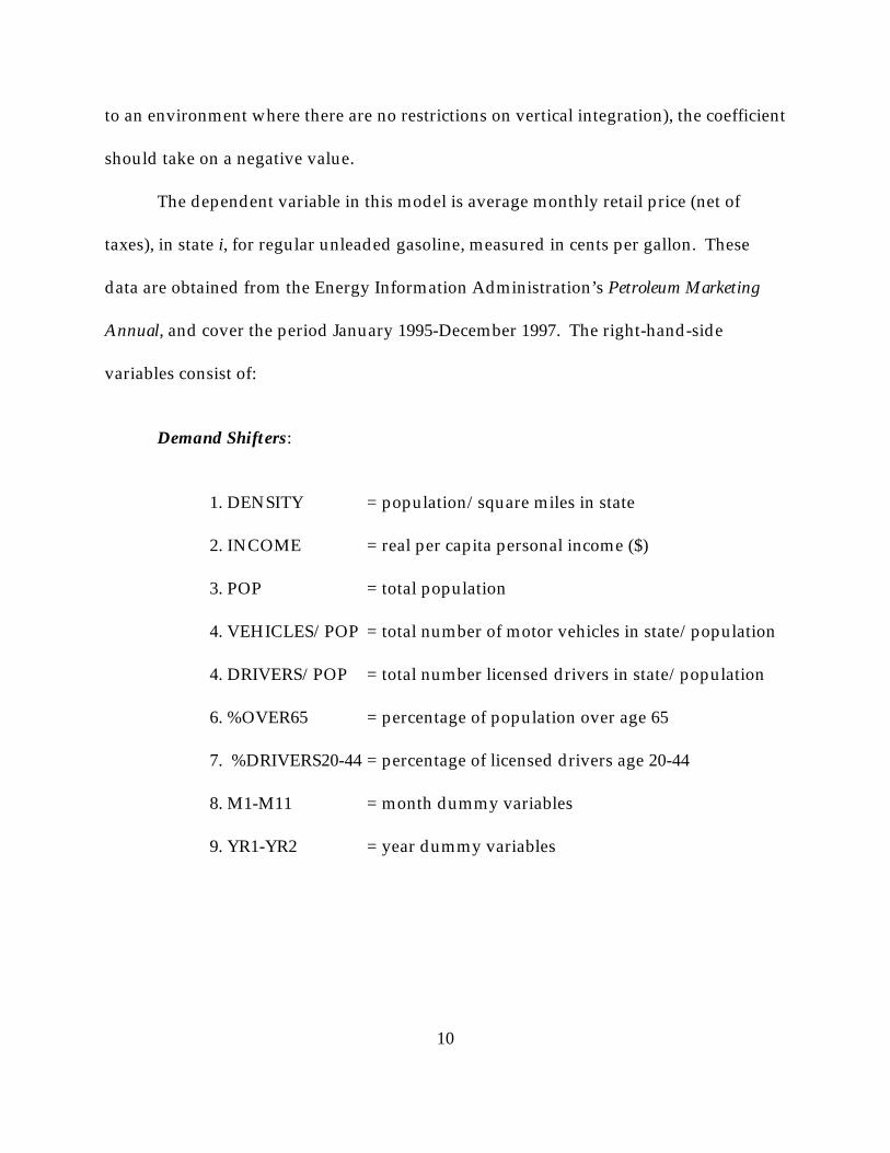
The dependent variable in this model is average monthly retail price (net of

taxes), in state i, for regular unleaded gasoline, measured in cents per gallon. These

data are obtained from the Energy Information Administration’s Petroleum Marketing

Annual, and cover the period January 1995-December 1997. The right-hand-side

variables consist of:

Demand Shifters:

1. DENSITY = population/square miles in state

2. INCOME = real per capita personal income ($)

3. POP = total population

4. VEHICLES/POP = total number of motor vehicles in state/population

4. DRIVERS/POP = total number licensed drivers in state/population

6. %OVER65 = percentage of population over age 65

7. %DRIVERS20-44 = percentage of licensed drivers age 20-44

8. M1-M11 = month dummy variables

9. YR1-YR2 = year dummy variables

14 To compute a heating or cooling degree day, add the high and lowtemperature for a given day. Divide the result by 2 to get the average temperature, andsubtract 65. If negative, this result is termed “heating degree days;” if positive, “coolingdegree days.” Thus, if on a given day the high temperature equaled 50, and the low 30,that day had 25 heating degree days.

11

Cost Shifters:

1. WAGERATE = real hourly earnings for retail employees in state($/hour)

2. TRANSPORT = real imputed transportation cost (see discussionbelow), (¢/gallon)

3. CRUDE = real spot price of West Texas Intermediate crude oil($/bbl.)

4. REFORMGAS = percentage of gasoline sold satisfying reformulatedgasoline (RFG) requirements

5. OXYGENGAS = percentage of gasoline sold satisfying winteroxygenated gasoline requirements

6. HEATINGDAYS = heating degree days in Census region14

7. CARBGAS = dummy variable (= 1 if state = California andmonth/year $ May 1996) to reflect imposition ofCalifornia Air Resources Board refining standard

8. WEST = dummy variable for states west of Rockies(California, Oregon, Washington, Idaho, Montana,Wyoming, Nevada, Arizona, New Mexico, Colorado,and Utah);

9. NE = dummy variable for Pennsylvania, New Jersey,NewYork, and the New England states)

10. AK , HI = dummy variables for Alaska and Hawaii

15 See Espey (1996, 1998) and Lin (1985).

12

Regulatory Variables:

1. DIVORCE = 1 if state had divorcement regulation; 0 otherwise

2. SELFSERV = percentage of gasoline sold through self-servicepumps

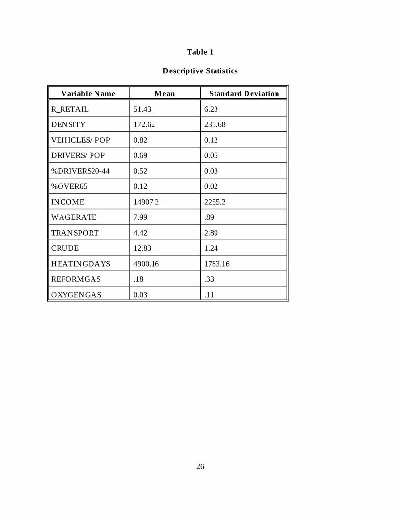
The means and standard deviations of these variables are presented in Table 1.

All nominal monetary values are deflated by the Consumer Price Index.

The basic specification of equation [1] reflects general theoretical considerations;

the specific choice of explanatory variables reflects the findings of previously published

estimates of gasoline demand.15 Economic theory implies that gasoline demand in an

area will depend in significant part upon the characteristics of the population living in

that area. These population characteristics include total population size (POP); average

per capita real income (INCOME); age distribution (%OVER65); vehicle ownership

(VEHICLES/POP); and driving licensure (DRIVERS/POP). It is expected that gasoline

demand (hence price) should increase with income, vehicle ownership, and licensure,

and decline with population age.

Previous researchers (e.g., Lin et al., 1985) also have found that gasoline demand

is influenced significantly by the population density (DENSITY). The impact of

increased density on price is ambiguous a priori. Travel demand, hence derived

gasoline demand, should fall as the population is increasingly concentrated in smaller

16 Dealers’ costs also might be a function of population density. Ceteris paribus,increased density might result in increased volume at a smaller number of dealers,allowing the latter to exploit economies of scale in retailing.

13

areas; moreover, there tend to be more alternative transportation modes available (e.g.,

buses) in densely populated areas. Additionally, increased population density likely

reduces costs of transporting fuel from the wholesale “rack” to retailers (since increased

population density likely will be associated with increased station density). Ceteris

paribus, these effects should induce a negative relationship between density and price.16

Conversely, increased population density also leads to traffic congestion, hence

increased fuel consumption per mile traveled, and higher land rental values. Both of

these factors should contribute to higher fuel prices.

Last, month dummies are included to control for the substantial seasonal

component of gasoline demand (see, e.g., Borenstein and Shepard, 1996, p. 440); year

dummies are included to control for unobservable determinants of price that vary

intertemporally, but not cross-sectionally.

Equation [1] also incorporates exogenous determinants of cost. Obviously, a

major determinant of gasoline costs is the price of crude oil. Following Borenstein and

Shepard (1996), I use the price of West Texas Intermediate crude as the relevant price

(although similar results are obtained when other spot prices (e.g., Brent crude) are

used). It is well documented that retail prices respond to crude prices with a lag

17 Ideally, one also would like to control for the cost of transporting crude oilfrom the field to the refinery. Because I lack direct measures of these costs, I insteadcontrol for crude transport price variation with four dummy variables: NE (equal toone for Pennsylvania, New Jersey, NewYork, and the New England states); WEST(equal to one for California, Oregon, Washington, Idaho, Montana, Wyoming, Nevada,Arizona, New Mexico, Colorado, and Utah); HI (equal to one for Hawaii), and AK(equal to one for Alaska).

18 A priori, it is not clear what sign the coefficient on HEATINGDAYS shouldhave. According to Scheffman and Spiller (1987, p. 136) and Borenstein et al. (1997, p.316), gasoline is refined as a by-product of home heating oil. Heating oil and gasolineare complements in production (i.e., increasing the output of heating oil also leads to anincrease in gasoline production), but substitutes in transportation (i.e., when heating oilis in high demand, a greater amount of transportation capacity is allocated to heatingoil).

14

(Borenstein et al., 1997); accordingly, I include current and lagged values of the crude

price as regressors.17

Production and transportation costs of gasoline also will be affected by the

demand for jointly produced products, such as home heating oil, the demand for which

is weather-determined.18 Accordingly, like Scheffman and Spiller (1987) and Borenstein

et al.(1997), I include the number of heating degree days (HEATINGDAYS) as an

exogenous determinant of gasoline production costs.

Another potentially important determinant of cross-sectional variation in

gasoline prices are environmental regulations that affect gasoline production costs. The

Clean Air Act Amendments of 1990 contained two primary requirements for cleaner

gasoline. The first of these is the reformulated gasoline (RFG) program, which requires

cleaner-burning RFG to be sold in the nine (now ten) worst “ozone nonattainment”

19 The original areas are Baltimore, Chicago, Hartford, Houston, Los Angeles,Milwaukee, New York, Philadelphia, and San Diego. Later, Sacramento was added tothis list.

15

areas, beginning January 1, 1995.19 In addition to the nine cities where RFG was

mandated, a number of other cities adopted the RFG program voluntarily. Because

RFG is more expensive to refine than ordinary gasoline, I include as an explanatory

variable (REFORMGAS) the percentage of gasoline sold that satisfies the reformulated

gasoline requirements.

The 1990 Clean Air Act Amendments also require the sale of oxygenated

gasoline during the winter months (usually November through February) in those areas

designated as carbon monoxide nonattainment areas. To control for the cost impact of

this requirement, I include a variable (OXYGENGAS) equal to the percentage of

gasoline sold that fulfills the oxygenated gasoline standards.

A third regulatory variable reflects the special reformulated gasoline program

instituted in California in 1996. Like the Federal RFG program, the California Air

Resources Board (CARB) standard is designed to reduce emissions of volatile organic

compounds and nitrogen oxides, both of which contribute to the creation of ground-

level ozone. The CARB-standard gasoline is refined to a different standard than the

RFG gas produced for the other nonattainment areas, and the requisite production

technology has been embodied in a relatively small number of refineries. At the time

the CARB requirements were imposed, it was estimated that the standards would add

20 See the CAL/EPA Factsheet at www .calepa . ca. gov /publications /factsheets/1997 /cleangas.htm.

21 For western states, I use the Los Angeles spot price. For midwest andsoutheastern states, I use the Gulf Coast spot price. For states in the Northeast, I use theNew York Harbor spot price.

16

5¢ to 15¢/gallon to the production cost of gasoline.20 To control for the impact of this

regulation on equilibrium prices, I include a dummy variable (CARBGAS) that takes on

a value of 1 for May 1996 and all subsequent periods for all California observations.

Because the production costs of CARB gasoline are thought to have fallen over time, I

also interact CARBGAS with a year dummy (equal to 1 for 1997).

A final determinant of the cost of retail gasoline is the transportation cost of

shipping the gasoline from the refinery to the dealer. Typically, bulk gasoline is

shipped either by pipeline or water transportation from the refinery gate to the

wholesale supply terminals, from which the gasoline is dispensed into tanker trucks for

final delivery to the retail dealer. Ideally, we would like to incorporate a direct measure

of these transportation costs into the empirical analysis. While interstate oil pipeline

tariffs are filed with the Federal Energy Regulatory Commission, and are thus publicly

available, there is no comparable source of public information for intrastate pipelines or

for spot tanker/barge rates. As an alternative, I impute the cost of transporting

gasoline from the refinery to the terminal (TRANSPORT) as the difference between a

spot refinery price and the average terminal (or “rack”) price for each state, as reported

by the Energy Information Administration.21

22 Other panel data estimation procedures, such as OLS with state-specificdummy variables (i.e., a fixed-effects model) are precluded by the fact that there is nowithin-state variation in the regulatory variables for the sample period used here.

17

yit ' Xitß % eit, eit ' ?ei,t&1 % ? it, ? it-(0,s 2I)

IV. Empirical Findings

The parameters of equation [1] are estimated with state-level monthly data for

the period January 1995 - December 1997. Because of the likely existence of serial

correlation of the disturbances within each state, I estimate equation [1] using a feasible

generalized least squares (FGLS) procedure that assumes a common autocorrelation

parameter across states.22 That is, I assume equation [1] takes the following form:

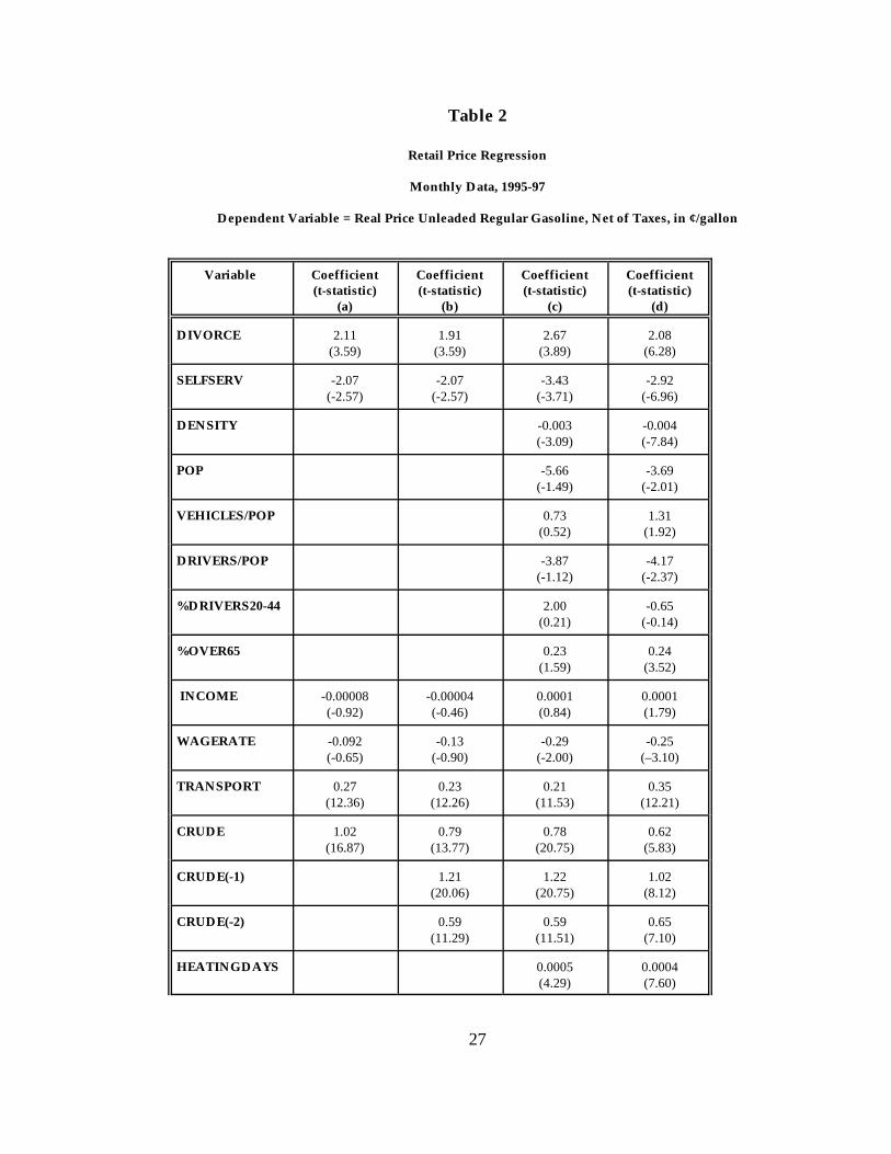
Table 2 presents several sets of estimated FGLS parameters of the gasoline price

equation. Column (a) presents a restricted version of equation [1], with only the most

basic demand and cost shifters included as explanatory variables. Column (b) adds

lagged crude prices to the equation; Column (c) adds other characteristics of the market

(e.g., per capita motor vehicle ownership). Column (d) presents OLS estimates of the

fully specified version of the pricing equation.

23 Exceptions are WAGERATE and %DRIVERS20-44. In neither case can wereject the null hypothesis that the true parameter is equal to zero.

24 Contrary to expectations, however, the coefficient on YR3*CARBGAS ispositive, suggesting that the cost of refining CARB standard gasoline rose, rather thanfell, over the course of the sample period.

18

The coefficients on most of the exogenous variables have signs consistent with

prior expectations.23 Current and lagged crude prices (CRUDE, CRUDE_1, CRUDE_2)

are positively related to retail prices, as are the imputed transportation costs

(TRANSPORT) and two of the three reformulated gasoline programs (OXYGENGAS

and CARBGAS).24 Increased population density (DENSITY) is negatively related to

price. Motor vehicle ownership (VEHICLES/POP), income (INCOME), and proportion

of drivers aged 20 to 44 (%DRIVERS20-44) are all positively related to retail price,

although none are different from zero at conventional levels of statistical significance.

Some of these controls (DRIVERS/POP, %OVER65, and WAGERATE) have

coefficients with unexpected signs, but only in the case of WAGERATE is the coefficient

statistically significant. The coefficient on heating degree days (HEATINGDAYS) is

positive and statistically significant.

The parameter estimates presented in Table 2 provide a clear pattern of evidence

suggesting that retail prices are 2¢ -3¢ per gallon higher in states with divorcement laws

than in states without such restrictions; the 95 percent confidence interval on the

estimated DIVORCE parameter in column (c), the fully specified version of model

estimated with the FGLS procedure, is approximately 1.3¢ to 4¢ per gallon. The null

25 Shepard (1993, p. 67) reports that the average open-dealer station had thecapacity to serve 3.6 cars at a time, versus 5 or more cars at other station types. In hersample, approximately 75 percent of the open-dealers had only a single island, whereasonly about 30 percent of the other stations were single island.

26 Shepard (1993, p. 68) reports that less than half of the open-dealers had been(continued...)

19

hypothesis that divorcement laws have no effect on retail prices can be rejected at the 1

percent significance level.

Divorcement statutes thus appear to have had the effect of increasing

equilibrium retail prices. It is difficult to construct a procompetitive characterization of

this result. One possibility is that there is some unobserved (by the econometrician)

average quality difference between dealers in divorcement and nondivorcement states

that consumers value at (approximately) 2.7¢ per gallon. While this possibility is, by

definition, untestable (if we could observe all relevant aspects of quality we would

include this information in the form of additional regressors), it would seem unlikely,

given available empirical information on the characteristics of company-owned versus

independently-owned stations. Existing research suggests the former are more likely to

have characteristics valued by gasoline purchasers than the latter. For example,

Shepard (1993) found that in her sample, company-owned stations tended to have

greater sales capacity than independently-owned stations;25 other things equal, greater

capacity suggests less time spent in a queue waiting for an open pump. Shepard also

reported that the independent open-dealer stations tended to have older physical plants

than other stations;26 this suggests, among other things, that the company-owned and

26 (...continued)remodeled in the 3-year period preceding the collection of her data; by contrast, morethan two-thirds of the other stations had undertaken some remodeling during thisperiod.

27 Source: National Petroleum News, Mid-June 1994.

20

lessee-dealer stations may tend to have newer restrooms and other facilities valued by

customers. In earlier research, Barron and Umbeck (1984, p. 324) found that stations

directly affected by divorcement reduced their hours of operation substantially after

they were converted from company-owned to dealer-owned facilities. Slade (1998,

Table 7) presents similar evidence; she found (via estimation of probit analysis of the

type of contract governing the refiner-retailer relationship) that hours of operation was

positively related to the probability that a station’s price was set by the refiner.

The parameter estimates in Table 2 also strongly indicate that, as one might

expect, prices vary considerably depending on the quantity of gasoline sold through

self-service pumps. In 1993, the last year for which data are available, almost 90 percent

of gasoline is sold as “self-serve” in the states where self-service is legal.27 This means

that in those states where self-service is banned (New Jersey and Oregon), the price of

unleaded regular gasoline is more than 3¢ per gallon higher, as shown in column (c),

than where it is not banned.

Using quantity data from the Energy Information Administration, price data

from the Lundberg Survey, and elasticity estimates from Espey (1998), we can

approximate the increase in consumers’ surplus that would arise from eliminating

21

divorcment regulations. Espey (1998, p. 279) provides estimates of the long-run price

elasticity of gasoline demand that range from 0 to -2.72 (median = -0.43). Using these

estimates, and annual volume data from the EIA (1999), we can compute the quantity

increases that would be induced by the predicted 2.7¢/gallon price reduction that

would accompany a relaxation of the divorcement restrictions. With this information, it

is straightforward to calculate the attendant increase in Marshallian consumer surplus,

which ranges from $111.4 million (assuming completely inelastic demand) to $115.4

million (assuming an elasticity of -2.72, Espey’s upper bound). For the median elasticity

estimate (? =-0.43), the corresponding surplus increase is approximately $112.0 million.

Calculated at the upper bound of the 95 percent confidence interval on DIVORCE

(4.02¢/gallon), the increase in surplus (evaluated at ? = -0.43) rises to over $112 million

annually.

It should be noted that these estimates are a lower bound on the welfare increase

that would result from deregulation of the refiner-retailer relationship. These

calculations correspond to the consumption of unleaded regular gasoline. Though we

have not estimated the effects of divorcement deregulation for the price and quantity of

mid-grade and premium fuel, it is quite likely that deregulation would engender

decreases in the prices of these products as well. Given that these higher-grade fuels

account for almost one-third of total gasoline sales, the consumer surplus associated

with these price changes would be substantial.

22

V. Conclusion

Although divorcement regulation has been imposed in only six states, there is

recurrent interest in this policy, particularly in areas (e.g., San Francisco, San Diego)

where retail prices appear “inexplicably” high (Goldstein, Gold, and Kleit, 1998;

Borenstein and Gilbert, 1993). As noted in the introduction, while it is possible

theoretically for vertical integration to result in noncompetitive equilibria, previous

empirical studies of divorcement not only fail to show that such policies result in lower

prices, they indicate strongly that divorcement results in prices significantly higher than

would have obtained had no such restrictions been imposed. This suggests that the

integration of refiners and retailers is a source of economic efficiency that is foregone

when integration is restricted or proscribed.

The analysis presented here reaffirms these earlier findings. Using state-level

data for the middle-1990s, I find that divorcement regulations increased the retail price

of unleaded regular gasoline by more than 2.7¢ per gallon. While this number might

seem small, it must be borne in mind, as Borenstein and Gilbert (1993) emphasize, that a

relatively small distortion can translate into a rather sizable aggregate welfare loss in a

large market. Annual retail sales of gasoline exceed $147 billion per year. Were

divorcement policies imposed via national legislation (as has been proposed in recent

years), the annual consumer welfare loss could come to approximately $2.5 billion per

year. This is a large price to pay for a policy having no evident benefits.

23

References

Barron, John and John Umbeck, “The Effects of Different Contractual Arrangements: The Case of Retail Gasoline Markets,” Journal of Law & Economics 27 (1984), 313-28.

Barron, John, Mark Loewenstein, and John Umbeck, “Predatory Pricing: The Case of theRetail Gasoline Market,” Contemporary Policy Issues 3 (1985), 130-39.

Bonanno, Giacomo, and John Vickers, “Vertical Separation,” Journal of Industrial Economics36 (1988), 257-65.

Borenstein, Severin, and Richard Gilbert, “Uncle Sam at the Gas Pump: Causes andConsequences of Regulating Gasoline Distribution,” Regulation (1993), 63-75.

Borenstein, Severin, A. Colin Cameron, and Richard Gilbert, “ Do Gasoline Prices RespondAsymetrically to Crude Oil Price Changes?,” Quarterly Journal of Economics 112 (1997), 305-39.

Borenstein, Severin and Andrea Shepard, “Dynamic Pricing in Retail Gasoline Markets,”RAND Journal of Economics 27 (1996), 429-51.

Coase, Ronald, “The Theory of the Firm,” Economica n.s. 4 (1937), 386-405.

Energy Information Administration, Petroleum Marketing Annual, 1999.

Espey, Molly, “Explaining the Variation in Elasticity Estimates of Gasoline Demand in theUnited States: A Meta-Analysis,” Energy Journal 17 (1996), 49-60.

____________. “Gasoline Demand Revisited: An International Meta-Analysis ofElasticities,” Energy Economics 20 (1998), 273-95.

Goldstein, Larry, Ron Gold, and Andrew Kleit, “Divorced From the Facts: Retail GasolineDivorcement Redux,” Oil & Gas Journal, November 9, 1998, 27-34.

Hart, Oliver, and Jean Tirole, “Vertical Integration and Market Foreclosure,” BrookingsPapers on Economic Activity, 1990, 205-86.

Honeycutt, T. Crawford, “Competition in Controlled and Uncontrolled Gasoline Markets,”Contemporary Policy Issues 3 (1985), 105-39.

24

Klein, Benjamin, Robert Crawford, and Armen Alchian, “Vertical Integration,Appropriable Rents, and the Competitive Contracting Process,” Journal of Law & Economics21 (1978), 297-326.

Klein, Benjamin, “Vertical Integration as Organizational Ownership: The Fisher Body-General Motors Relationship Revisited,” Journal of Law, Economics, & Organization (1988),199-213.

Lin, An Loh et al., “State Gasoline Consumption in the USA: An Econometric Analysis,”Energy Economics 7 (1985), 29-36.

Mallela, Parthasaradhi and Babu Nahata, “Theory of Vertical Control With VariableProportions,” Journal of Political Economy 88 (1980), 1009-25.

Monteverde, Kirk, and David J. Teece, “Supplier Switching Costs and Vertical Integrationin the Automobile Industry,” 13 Bell Journal of Economics (1982), 206-13.

_________________________, “Appropriable Rents and Quasi-Vertical Integration,” 25Journal of Law & Economics 25 (1982) 321-28.

Ordover, Janusz et al., “Equilibrium Vertical Foreclosure,” American Economic Review 80(1990), 127-42.

Reiffen, David and Michael Vita, “Is There New Thinking on Vertical Mergers?,” AntitrustLaw Journal 63 (1995), 917-41.

Rey, Patrick and Joseph Stiglitz, “The Role of Exclusive Territories in Producers’Competition,” RAND Journal of Economics 26 (1995), 431-51.

Salinger, Michael, ”Vertical Mergers and Market Foreclosure,” Quarterly Journal ofEconomics 103 (1988), 345-56.

Shepard, Andrea “Pricing Behavior and Vertical Contracts in Retail Markets,” AmericanEconomic Review (Papers and Proceedings), 80 (1990), 427-31.

_________________, “Contractual Form, Retail Price, and Asset Characteristics,” RANDJournal of Economics 24 (1993), 58-77.

Slade, Margaret, “Strategic Motives for Vertical Separation,” Journal of Law, Economics, &Organization 14 (1998), 84-113.

25

Spengler, Joseph, “Vertical Integration and Antitrust Policy,” Journal of Political Economy58 (1950), 347-52.

Tirole, Jean, The Theory of Industrial Organization, (Cambridge: MIT Press),1988.

Westfield, J. Fred, “Vertical Integration: Does Product Price Rise or Fall?,” AmericanEconomic Review 71 (1981), 334-46.

26

Table 1

Descriptive Statistics

Variable Name Mean Standard Deviation

R_RETAIL 51.43 6.23

DENSITY 172.62 235.68

VEHICLES/POP 0.82 0.12

DRIVERS/POP 0.69 0.05

%DRIVERS20-44 0.52 0.03

%OVER65 0.12 0.02

INCOME 14907.2 2255.2

WAGERATE 7.99 .89

TRANSPORT 4.42 2.89

CRUDE 12.83 1.24

HEATINGDAYS 4900.16 1783.16

REFORMGAS .18 .33

OXYGENGAS 0.03 .11

27

Table 2

Retail Price Regression

Monthly Data, 1995-97

Dependent Variable = Real Price Unleaded Regular Gasoline, Net of Taxes, in ¢/gallon

Variable Coefficient(t-statistic)

(a)

Coefficient(t-statistic)

(b)

Coefficient(t-statistic)

(c)

Coefficient(t-statistic)

(d)

DIVORCE 2.11(3.59)

1.91(3.59)

2.67(3.89)

2.08(6.28)

SELFSERV -2.07(-2.57)

-2.07(-2.57)

-3.43(-3.71)

-2.92(-6.96)

DENSITY -0.003(-3.09)

-0.004(-7.84)

POP -5.66(-1.49)

-3.69(-2.01)

VEHICLES/POP 0.73(0.52)

1.31(1.92)

DRIVERS/POP -3.87(-1.12)

-4.17(-2.37)

%DRIVERS20-44 2.00(0.21)

-0.65(-0.14)

%OVER65 0.23(1.59)

0.24(3.52)

INCOME -0.00008(-0.92)

-0.00004(-0.46)

0.0001(0.84)

0.0001(1.79)

WAGERATE -0.092(-0.65)

-0.13(-0.90)

-0.29(-2.00)

-0.25(–3.10)

TRANSPORT 0.27(12.36)

0.23(12.26)

0.21(11.53)

0.35(12.21)

CRUDE 1.02(16.87)

0.79(13.77)

0.78(20.75)

0.62(5.83)

CRUDE(-1) 1.21(20.06)

1.22(20.75)

1.02(8.12)

CRUDE(-2) 0.59(11.29)

0.59(11.51)

0.65(7.10)

HEATINGDAYS 0.0005(4.29)

0.0004(7.60)

Variable Coefficient(t-statistic)

(a)

Coefficient(t-statistic)

(b)

Coefficient(t-statistic)

(c)

Coefficient(t-statistic)

(d)

28

REFORMGAS -0.41(-1.37)

-0.45(-1.74)

-0.19(-0.72)

1.06(3.32)

OXYGENGAS 1.29(2.06)

0.75(1.27)

0.56(0.96)

3.02(4.60)

CARBGAS 1.21(0.98)

0.54(0.48)

1.95(1.67)

0.34(0.35)

CARBGAS*YR3 0.37(0.26)

1.32(1.06)

1.92(1.54)

0.60(0.55)

AK 24.66(27.82)

24.48(25.76)

26.26(20.52)

25.07(41.09)

HI 15.38(15.85)

15.97(15.45)

15.85(13.71)

14.91(24.05)

WEST 5.79(18.09)

5.80(17.13)

5.89(15.29)

5.60(30.14)

NE 2.55(5.83)

2.39(5.11)

1.75(3.27)

1.70(6.91)

CONSTANT 37.36(21.23)

16.44(8.12)

13.29(2.24)

16.94(5.61)

autocorrelationcoefficient

0.6865 0.7571 0.7684 na

R2 na na na 0.85

Log Likelihood -3474.48 -2976.13 -2934.36 na

Coefficients in columns (a)-(c) estimated with feasible generalized least squares assuming homoskedasticityand a constant autocorrelation coefficient across states. Coefficients in column (d) estimated with ordinaryleast squares. Coefficients on month and year dummies not shown.