Reinhard Blutner1

Linear Algebra and Geometric Approaches to Meaning

3b. Distributed Semantics

Reinhard Blutner

Universiteit van Amsterdam

ESSLLI Summer School 2011, Ljubljana

August 1 – August 7, 2011

Acknowledgement

• We thank Stefan Evert for allowing us to use some of his slides presented at the “Tandem Workshop on Optimality in Language and Geometric Approaches to Cognition” (Berlin, December 11-13, 2010) for parts of this course.

• Links– http://wordspace.collocations.de/doku.php/course:start– http://www.blutner.de/tandem/index.htm

Reinhard Blutner2

Reinhard Blutner3

1

1. Meaning and Distribution

2. Distributional semantic models

3. Word vectors and search engines

4. Latent semantic analysis

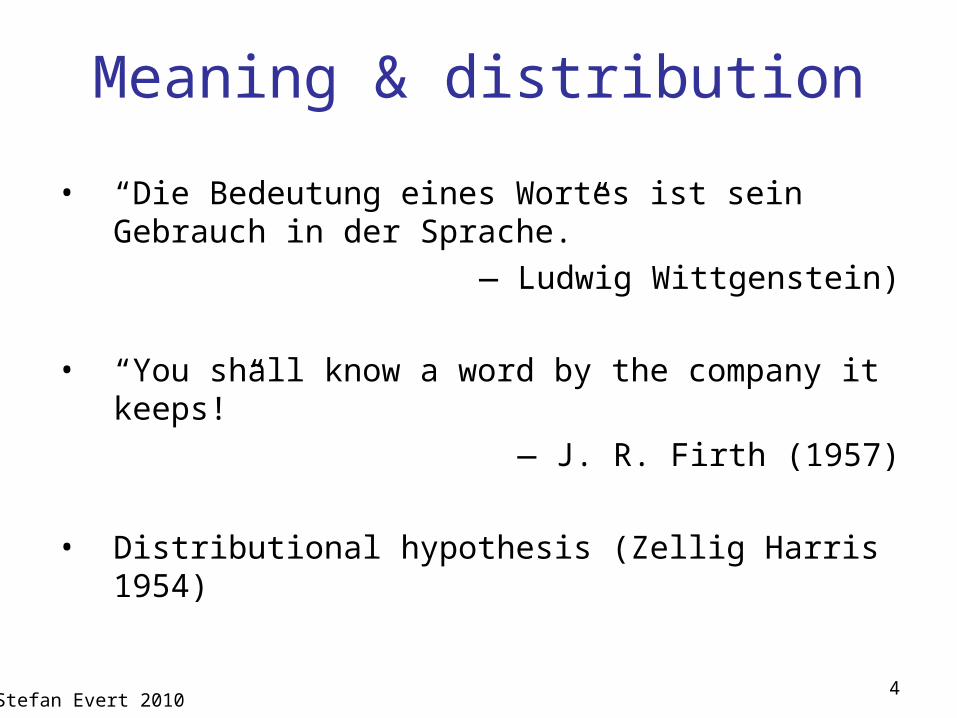
Meaning & distribution

• “Die Bedeutung eines Wortes ist sein Gebrauch in der Sprache.”

— Ludwig Wittgenstein)

• “You shall know a word by the company it keeps!”

— J. R. Firth (1957)

• Distributional hypothesis (Zellig Harris 1954)

Stefan Evert 20104

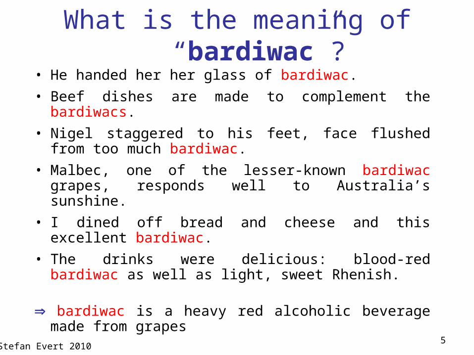
What is the meaning of “bardiwac”?

• He handed her her glass of bardiwac.

• Beef dishes are made to complement the bardiwacs.

• Nigel staggered to his feet, face flushed from too much bardiwac.

• Malbec, one of the lesser-known bardiwac grapes, responds well to Australia’s sunshine.

• I dined off bread and cheese and this excellent bardiwac.

• The drinks were delicious: blood-red bardiwac as well as light, sweet Rhenish.

bardiwac is a heavy red alcoholic beverage made from grapes

Stefan Evert 20105

The Distributional Hypothesis

• DH (Lenci 2008)– At least certain aspects of the meaning of lexical

expressions depend on their distributional properties in the linguistic contexts

– The degree of semantic similarity between two linguistic expressions and is a function of the similarity of the linguistic contexts in which and can appear

• Weak and strong DH– Weak view as a quantitative method for semantic

analysis and lexical resource induction– Strong view as a cognitive hypothesis about the form

and origin of semantic representations; assuming that word distributions in context play a specific causal role in forming meaning representations.

Reinhard Blutner6

Geometric interpretation

• row vector xdog describes usage of word dog in the corpus

• can be seen as coordinates of point in n-dimensional Euclidean space Rn

7Stefan Evert 2010

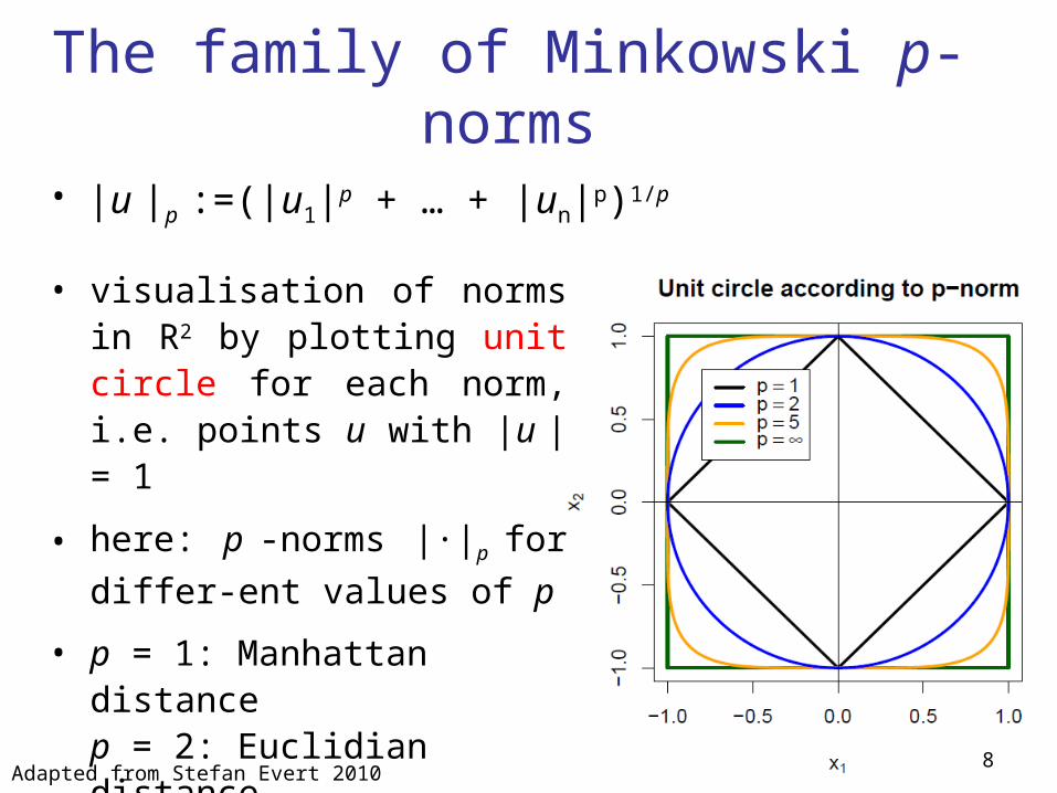
The family of Minkowski p-norms

Adapted from Stefan Evert 20108

• .

• visualisation of normsin R2 by plotting unitcircle for each norm, i.e. points u with |u | = 1

• here: p -norms |·|p for

differ-ent values of p

• p = 1: Manhattan distancep = 2: Euclidian distancep : maximum distance

|u |p :=(|u1|p + … + |un|p)1/p

Distance and similarity

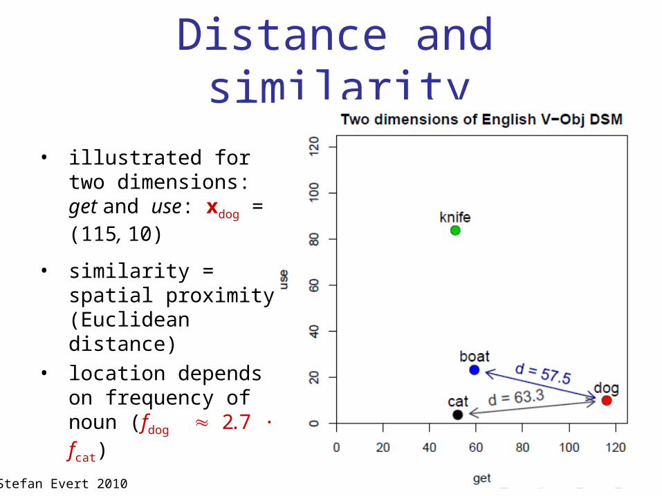
• illustrated for two dimensions: get and use: xdog = (115, 10)

• similarity = spatial proximity (Euclidean distance)

• location depends on frequency of noun (fdog 2.7 · fcat)

9Stefan Evert 2010

Angle and similarity

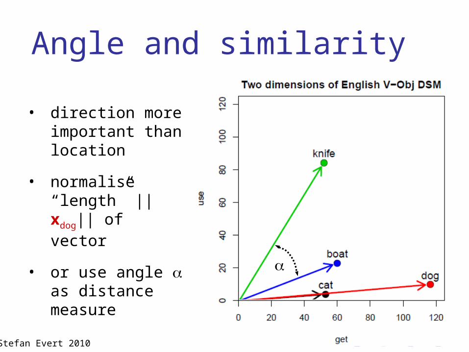
• direction more important than location

• normalise “length” ||xdog|| of vector

• or use angle as distance measure

10Stefan Evert 2010

Reinhard Blutner11

2

1. Meaning and Distribution

2. Distributional semantic models

3. Word vectors and search engines

4. Latent semantic analysis

A very brief history

• Introduced to computational linguistics in early 1990s following the probabilistic revolution (Schütze 1992, 1998)

• Other early work in psychology (Landauer and Dumais 1997; Lund and Burgess 1996)

- influenced by Latent Semantic Indexing (Dumais et al. 1988) and efficient software implementations (Berry 1992)

• Renewed interest in recent years

– see http://wordspace.collocations.de/doku.php/course:start

Adapted from Stefan Evert 201012

Some applications in computational linguistics

• Unsupervised part-of-speech induction (Schütze 1995)

• Word sense disambiguation (Schütze 1998)

• Synonym tasks & other language tests (Landauer and Dumais 1997; Turney et al. 2003)

• Ontology & wordnet expansion (Pantel et al. 2009)

• Probabilistic language models (Bengio et al. 2003)

• Subsymbolic input representation for neural networks

• Many other tasks in computational semantics: entailment detection, noun compound interpretation,…

Adapted from Stefan Evert 201013

Example: Word Space (Schütze)

• Corpus: 60 million words of news messages (New York Times News Service)

• Word-word co-occurrence matrix (20,000 target words & 2,000 context words as features)

• Row vector records how often each context word occurs close to the target word (co-occurrence)

• Co-occurrence window: left/right 50 words (Schütze 1998) or 1000 characters (Schütze 1992)

• Normalization -- determine “meaning” of a context

• Reduced to 100 Singular Value dimensions (mainly for efficiency)

Stefan Evert 201014

Clustering

15Adapted from Stefan Evert 2010

Semantic maps

16Adapted from Stefan Evert 2010

Reinhard Blutner17

3

1. Meaning and Distribution

2. Distributional semantic models

3. Word vectors and search engines

4. Latent semantic analysis

Basic references

• Dominic Widdows, Geometry of Meaning, CSLI, 2004

• Keith van Rijsbergen, The Geometry of Information Retrieval, Cambridge University Press, 2004

• D. Widdows & S. Peters, Word vectors and quantum logic, in MoL8, 2003.

Reinhard Blutner18

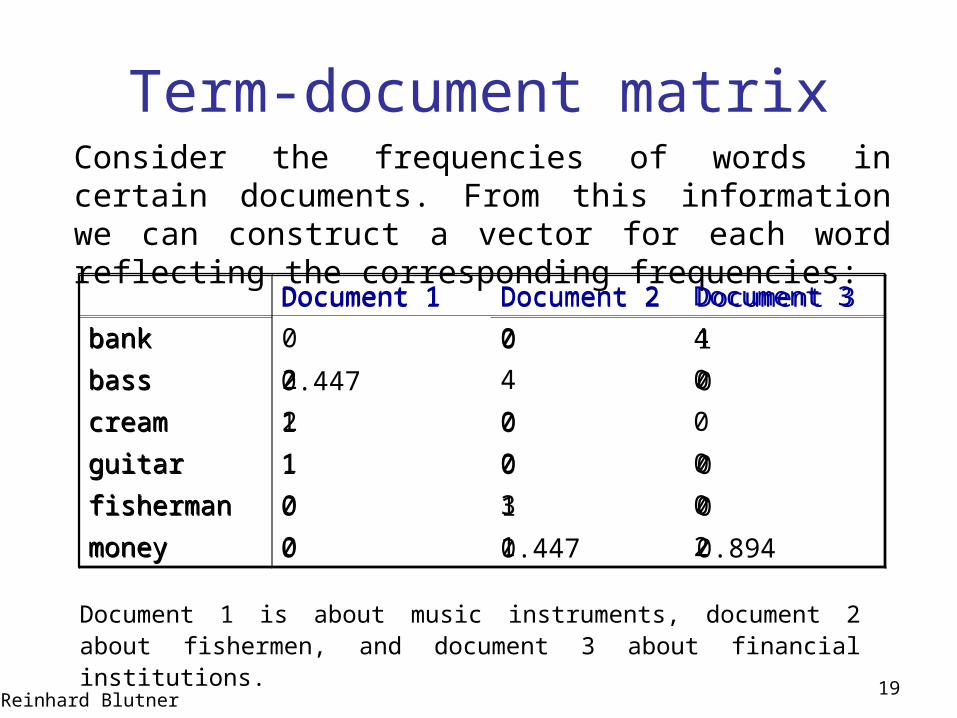
Term-document matrixConsider the frequencies of words in certain documents. From this information we can construct a vector for each word reflecting the corresponding frequencies:

Document 1 Document 2 Document 3

bank 0 0 1

bass 0.447 0.894 0

cream 1 0 0

guitar 1 0 0

fisherman 0 1 0

money 0 0.447 0.894

Document 1 is about music instruments, document 2 about fishermen, and document 3 about financial institutions.

Reinhard Blutner19

Document 1 Document 2 Document 3

bank 0 0 4

bass 2 4 0

cream 2 0 0

guitar 1 0 0

fisherman 0 3 0

money 0 1 2

Similarity Matrix (scalar product/cos )

bank bass cream guitar fisherman

money

bank 0 0 0 0 0.894

bass 0 0.447 0.447

0.894 0.400

cream 0 0.447

1 0 0

guitar 0 0.447

1 0 0

fisherman

0 0.894

0 0 0.447

money 0.894

0.400

0 0 0.447

Reinhard Blutner20

• Words such as bass are ambiguous (i. music instrument, ii. fish). If a user is only interested in one of these meanings, how are we to enable users to search for only the documents containing this meaning of the word?

• a NOT b = a – (a b) b

a NOT b is a vector that is orthogonal to b, i.e. (a NOT b ) b = 0

• bass NOT fisherman= (0.447 0.894 0) NOT (0 1 0) = (1 0 0)

Vector Negation

Reinhard Blutner21

Reducing dimensions using SVD

• Based on Singular Value decomposition

• Considering only the highest singular values reduces redundencies of the original matrix

• The approach can be thought as a version of decomposing words into semantic primitivesReinhard Blutner

22

Reinhard Blutner23

3

1. Meaning and Distribution

2. Distributional semantic models

3. Word vectors and search engines

4. Latent semantic analysis

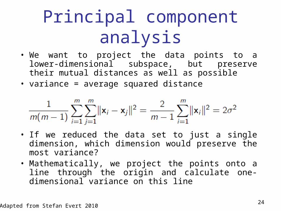
Principal component analysis

• We want to project the data points to a lower-dimensional subspace, but preserve their mutual distances as well as possible

• variance = average squared distance

• If we reduced the data set to just a single dimension, which dimension would preserve the most variance?

• Mathematically, we project the points onto a line through the origin and calculate one-dimensional variance on this line

24Adapted from Stefan Evert 2010

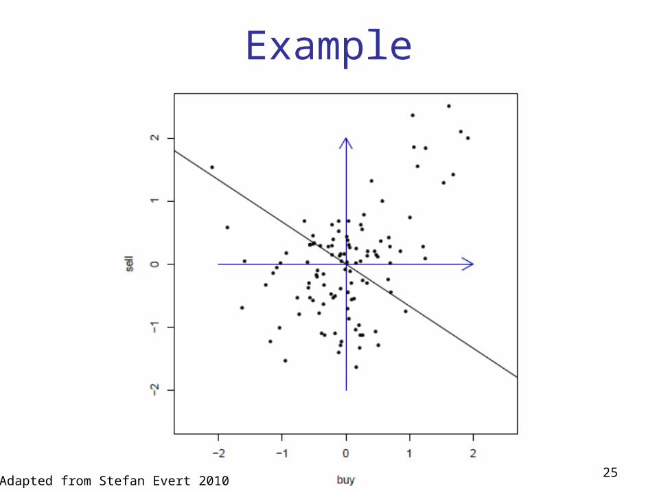
Example

25Adapted from Stefan Evert 2010

The covariance matrix

• Assume the distributional analysis gives a nm matrix M.

• With the help of the covariance matrix

is it possible to calculate the variance v2 of projections

on the unit vector v by the following formula:

v2 = vT C v (without proof)

• Orthogonal dimensions v1, v2, . . . partition variance:

• Use the eigenvectors of the covariance matrix C

26Adapted from Stefan Evert 2010

Principal components

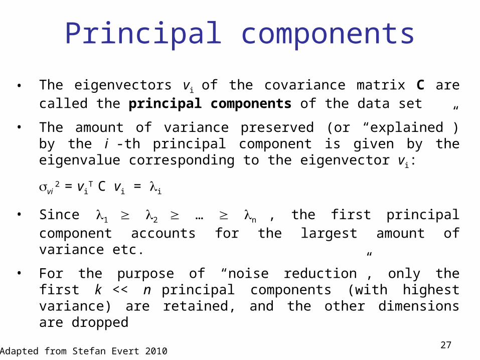
• The eigenvectors vi of the covariance matrix C are called the principal components of the data set

• The amount of variance preserved (or “explained”) by the i -th principal component is given by the eigenvalue corresponding to the eigenvector vi:

vi 2 = vi

T C vi = i

• Since 1 2 … n , the first principal component accounts for the largest amount of variance etc.

• For the purpose of “noise reduction”, only the first k << n principal components (with highest variance) are retained, and the other dimensions are dropped

27Adapted from Stefan Evert 2010

Singular Value Decomposition (SVD)• The SVD can be seen as a generalization of the

spectral theorem, which says that normal matrices can be unitarily diagonalized using a basis of eigenvectors, to arbitrary, not necessarily square, matrices.

• SVD: Any mn matrix A can be factorized as the product UV* of three matrixes where U is an mm unitary matrix over K (i.e., the columns of U are orthonormal), the matrix Σ is mn with nonnegative numbers on the diagonal (called the singular values) and zeros off the diagonal, and V* denotes the conjugate transpose of V, an nn unitary matrix over K. Such a factorization is called a singular-value decomposition of A.

Reinhard Blutner28

General scheme SVD

(This illustration assumes m > n, i.e. A has more rows than columns. For m < n, is a horizontal rectangle with diagonal elements 1, . . . , m.)

29Adapted from Stefan Evert 2010

SVD: Some links• http

://en.wikipedia.org/wiki/Singular_value_decomposition

• http://users.pandora.be/paul.larmuseau/SVD.htm (for per forming online computations)

• http://mathworld.wolfram.com/SingularValueDecomposition.html

• Distributed semantic model tutorial & other materials available from http://wordspace.collocations.de/

Reinhard Blutner30

Reinhard Blutner31

Conclusions

• At least certain aspects of the meaning of lexical expressions depend on their distributional properties in the linguistic contexts

• Weak distributional hypothesis as a quantitative method for semantic analysis and lexical resource induction

• PCA and SVD as methods to reduce the dimension of the primary semantic space.

• SVD as an empirical method for calculating relevant meaning components. When does it work and when not?

Appendix: Linear algebraic proof of SVD

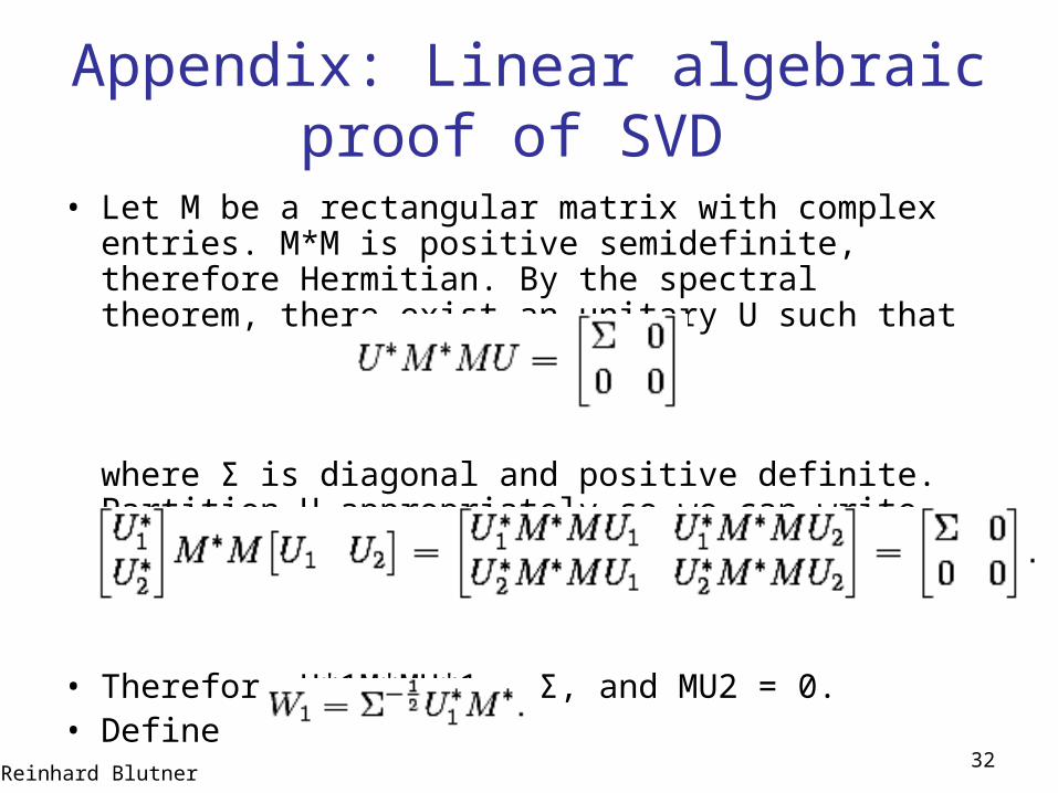
• Let M be a rectangular matrix with complex entries. M*M is positive semidefinite, therefore Hermitian. By the spectral theorem, there exist an unitary U such that

where Σ is diagonal and positive definite. Partition U appropriately so we can write

• Therefore U*1M*MU*1 = Σ, and MU2 = 0. • Define

Reinhard Blutner32

• Then

• We see that this is almost the desired result, except that W1 and U1 are not unitary in general. W1 is a partial isometry (W1W*1 = I ) while U1 is an isometry (U*1U1 = I ). To finish the argument, one simply has to "fill out" these matrices to obtain unitaries. U2 already does this for U1. Similarly, one can choose W2 such that

is unitary. Direct calculation shows

which is the desired result.

• Notice the argument could begin with diagonalizing MM* rather than M*M (This shows directly that MM* and M*M have the same non-zero eigenvalues).

Reinhard Blutner33