reinisch_85.511 1

85. 511 Solar Terrestrial Relations(Cravens, Physics of Solar Systems Plasmas, Cambridge U.P.)

• Lecture 1- Space Environment– Matter in Universe: 99.9% plasma– Plasma everywhere

• Solar Atmosphere

• Interplanetary Medium

• Planetary Magnetospheres

• Planetary Ionospheres

reinisch_85.511 2

Space Environment

• Plasma = + and – charged particles (ions, electrons) and neutral particles

• Forces on charges particles– Electric force FE = qE

– Magnetic force FB = qvxB

– Lorentz force F = qE + qvxB– Neutral forces mg,

1p

��������������

reinisch_85.511 3

Space Environment cont’d

• Solar wind

• Interplanetary magnetic field (IMF)– Tsyganenko model

• Magnetosphere– Dipole field??

reinisch_85.511 4

Interplanetary Space and MagnetosphereInterplanetary Space and Magnetosphere • Solar Wind. The SW is a collisionless supersonic (VSW > VS) plasma

that carries its own (solar) magnetic field with it. The Earth’s magnetic field presents a “hard” obstacle to the SW. The SW drapes around this obstacle forming a magnetic cavity that is shaped like a comet head and tail.

• Bow Shock. The bow shock is formed at x 12 RE sunward where pSW = pB. The SW decelerates at the bow shock becoming subsonic, but further downwind becomes supersonic again.

• Magnetosheath (note: Dr. Song is one of the world’s experts). Downwind from bow shock, the magnetosheath contains decelerated SW plasma. Some of this plasma fuses into the magnetosphere further along the tail.

• Magnetopause. Encloses the magnetosphere “shielding” it from the SW. Geocentric distance ~10 RE. Large current systems on the front (head) and the tail. Ne 50 cm-3.

• Magnetosphere. – Cusp, Plasmasphere, Ionosphere.

reinisch_85.511 5

Earth’s MagnetosphereEarth’s Magnetosphere 1. Magnetosphere. Volume inside magnetopause. Geomagnetic forces

dominate the motion of charged particles. Plasma originates from SW and the Earth’s ionosphere. SW enters in the polar cusp and along the tail.

2. Cusp (Cleft). SW entry point on the dayside. At ionospheric heights (300 km) it occupies a narrow latitudinal band near noon.

3. Plasma Sheet. Low density plasma originating in SW and ionosphere. But particles have much higher energy. Plasma flows into Earth’s atmosphere and forms the auroral ovals (borealis and australis).

4. Neutral Current Sheet. It is the separation between the earthward B-lines above (north) and the fieldline pointing away from the Earth below (south). Adawn-to-dusk current flows along the neutral current sheet, thus maintaining the oppositely directed magnetic fields (required/explained by Maxwell’s equations). At the “end” of the geomagnetic tail, the B-lines connect to the solar inter planetary magnetic field (IMF). This magnetic “reconnections” creates a voltage drop of ~100 kV creating currents of > 10 million amps. The potential drop projects down ionospheric heights creating a 100 kV voltage drop across the polar cap defining the dawn to dusk polar cap electric field.

reinisch_85.511 6

Earth’s Magnetosphere Earth’s Magnetosphere cont’dcont’d1. Van Allen Radiation Belts. Energetic particles near

the plasma sheet center flowing earthward get trapped in closed magnetic field lines forming the radiation belts. The trapped particles spiral along the closed magnetic field lines, bouncing back and forth between the northern and southern hemisphere. Electrons and protons (and some O ions from the ionosphere) in the frequency range 10-300 keV also have an azimuthal drift: electrons eastward, ions westward. This forms a current, the ring current.

2. Plasmasphere. A relatively high density plasma region closer to Earth, < 4 RE geocentric. Ne > 100 cm-3. Decrease in density at the “Carpenter knee”, I.e., the plasmapause (F. 2.12). The plasmasphere rotates with the Earth.

3. Ionosphere. Earth’s atmosphere ionized by solar UV

SwRI

NASA

reinisch_85.511 8

reinisch_85.511 9

reinisch_85.511 10

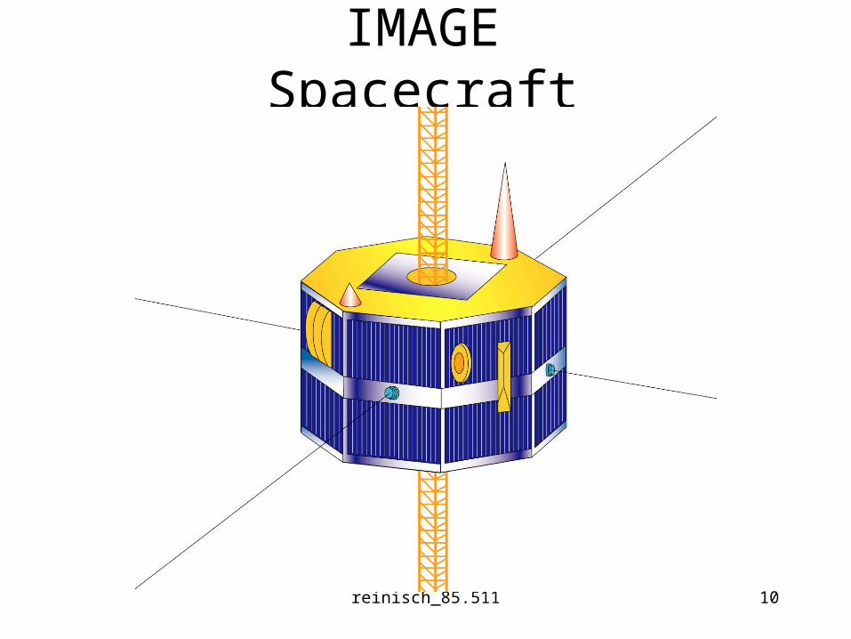
IMAGE Spacecraft

reinisch_85.511 11

25 March 2000Vandenburg AFB

Delta II Rocket

reinisch_85.511 12

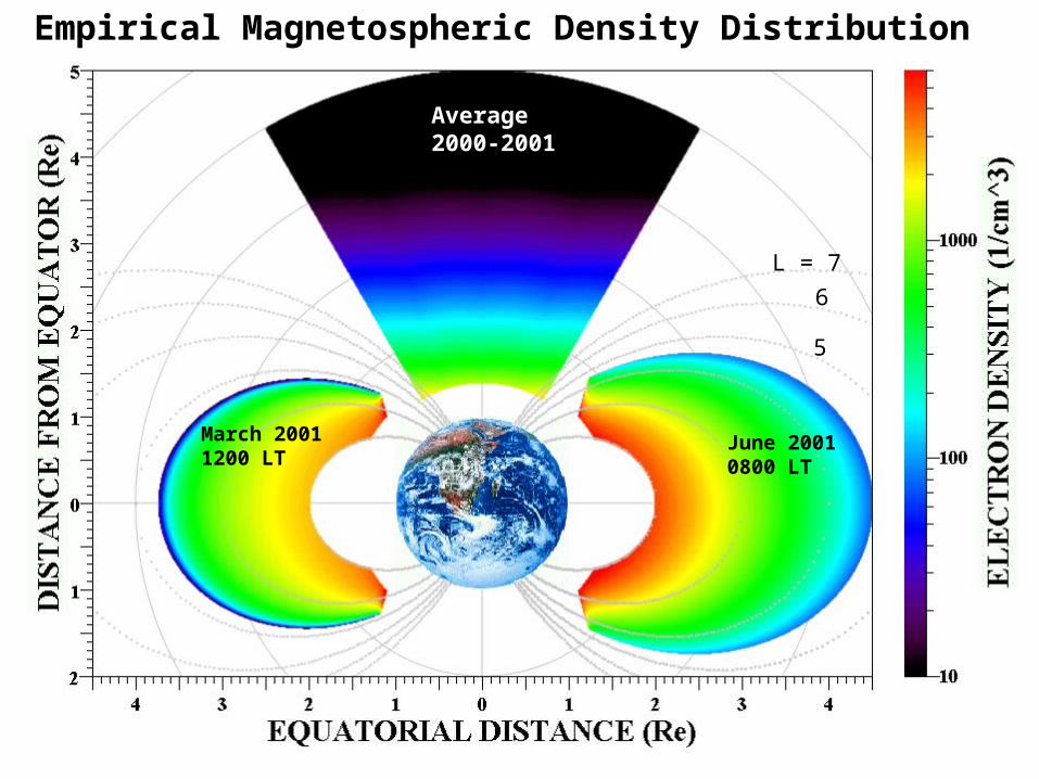
Empirical Magnetospheric Density Distribution

Average2000-2001

L = 7

6

5

June 20010800 LT

March 20011200 LT

reinisch_85.511 13

2.4-5 The Sun’s PlanetsPlanetsThe Planets’ Magnetospheres

Mercury

Venus (negligible, bow shock forms at ionopause)

Earth

Mars (very weak)

Jupiter

Saturn

Uranus

Neptune

reinisch_85.511 14

Plasma and Neutral ParametersPlasma and Neutral Parameters

Ne – electron density

Te,i,n –electron/ion/neutral temperature

Nn – neutral density

D – Debye length

ND – number of particles in Debye sphere

p – 2 x plasma frequency

c – 2 x cyclotron (gyro) frequency

r - gyroradius

12

02e

De

kTn e

343 eD D nN

122

0p

nem

c

e B

m

1

22 /

c

kT mmv

eBr

reinisch_85.511 15

Ch 2 - Kinetic TheoryTotal force on particle " " (Newton's second law):

, and

Sum of forces:

electromagnetic + gravity + pressure gradient + Coriolis + ...

In space plasma, the electromagnetic (Lorent

d dm

dt dt

v x

F v

3

z) force

is most important:

A full description of a real plasma system with N particles

requires 6N numbers at each time t. , .

q q x

10 0

F E v B

But N is large 10 to 10

reinisch_85.511 16

Particle Distribution Function

x y z

" " encompasses ordinary space ( ) and velocity space ( ),

i.e., independent coordinates (x,y,z,v , v ,v )

We consider only s-type particles (for example: electrons

Phase space

#m

)

, , lis

particles in Vf t

V

x v

x v

for volume element 0.

, , is the # of all type-s particles between

, , that have velocities beween

, , ,divided by .

s

x x y y z z

V

f t

x x y y z z

v v v v v v x y z

x v

reinisch_85.511 17

Density Function ns

3

3

If we add up all s-particles from all "velocity volume" elements

at location , we get the # of s-particles

per unit volume:

( , ) , , , ,

x y z

s s x y z s

d dv dv dv

n t f t dv dv dv f t d

v x

x x v x v v

reinisch_85.511 18

2.1.2 The Boltzmann EquationsHow can we determine the distribution function f ?

v

Answer: Solve the equation! Ha, Ha.

(2.6)

Approximate form of the collision terms is

2.8

Here is the "Maxwellian", introduc

s ss s

collision

s s sM

coll coll

sM

f ff f

t t

f f f

t

f

Boltzmann

v a

ed later,

and the average collision time.coll

reinisch_85.511 19

Total Derivative in Phase Space

v

v

So we can write (2.6) as

Considering only the em force (acceleration), we get;

.

Neglectin

phsp sss s

phsp

phsp s s

collisionphsp

s s ss s

collisions

D fff f

t D t

D f f

D t t

f q ff f

t m t

v a

v E v B

v

g the collision term, we get the equation:

0s ss s

s

f qf f

t m

Vlassov

v E v B

reinisch_85.511 20

Examples of Distribution Functions

0

0

0

Any number of distribution functions satisfies the Boltzmann equation.

1. Consider a gas of electrons all moving with

:

, ,

2. Consider a unifom gas , of ions, all having t

x

e o x x y z

u

f t n v u v v

n t n

v x

x v

x

0

0

22

0

0 0 0

22 2

0 0

0 0 0

0 002 2

0 0

he same speed :

, ,

, , , , sin

sin 4

, , 2.144 4

i

i i

i

v

f t A v v

n f t d f t v dvd d

A v v v dvd d Av

n nA f t v v

v v

v

x v

x v v x v

x v