rel grav tutorial

Introduction to Gravimetry

Conducting and ProcessingRelative Gravity Surveys

- A Brief Tutorial -

DIPL.-ING. TORBEN SCHÜLER

Institute of Geodesy and Navigation (IfEN)University FAF Munich, Germany

Conducting and Processing Relative Gravity Surveys 2

Table of Contents

1. CALIBRATION OF THE GRAVITY METER ........................................................... 3

1.1 Calibration Function and Calibration Table ................................................................................................ 3

1.2 Determination of the Calibration Function................................................................................................... 4

2. PLANNING AND CONDUCTING THE SURVEY.................................................... 5

2.1 Networks and Selection of Control Points..................................................................................................... 5

2.2 Station Description.......................................................................................................................................... 5

2.3 Preparation of the Survey............................................................................................................................... 6

2.4 Accomplishment of the Survey....................................................................................................................... 82.4.1 Survey Procedure and Drift Control .......................................................................................................... 82.4.2 Azimuth Dependency ................................................................................................................................ 82.4.3 Transport ................................................................................................................................................... 82.4.4 Counter Reading........................................................................................................................................ 9

2.5 Achievable Accuracy....................................................................................................................................... 9

3. PRE-PROCESSING OF DATA............................................................................. 11

4. ADJUSTMENT...................................................................................................... 13

4.1 Methods.......................................................................................................................................................... 13

4.2 Observation Equation................................................................................................................................... 13

4.3 Least Squares Adjustment............................................................................................................................ 14

5. BIBLIOGRAPHY................................................................................................... 15


1. Calibration of the Gravity Meter

1.1 Calibration Function and Calibration Table

The measurements are usually read in counter units (C. U. ) and have to be convertedto gravity units (usually µm/s2). For LACOSTE-ROMBERG gravity meters one counterunit roughly corresponds to one mGal1, but not precisely. The exact relation betweencounter unit measurements and gravity values is given by a calibration function whichis normally expressed time-independently:

( )zfg = 1.1

The calibration function can be separated into a polynomial part representing thelong wave components and a periodic part modeling the error of the dial via aFOURIER series and is to be applied for surveys of higher accuracy:

( ) ∑=

⋅=m

0n

nnpolynomial zpzf

1.2

( ) ( ) ( ) ( )∑∑==

ϕ−⋅ω⋅=⋅ω⋅+⋅ω⋅=l

1iiiiii

l

1iiiperiodic zcosazsinszcosczf 1.3

pn are polynomial coefficients, ci and si are amplitudes of cosine and sine terms,respectively, and ai as well as ϕi denote the same function using the amplitude/phaseangle-representation. In this way we yield a calibration function of the form

( ) ( ) ( )f z f z f zpolynomial periodic= + .

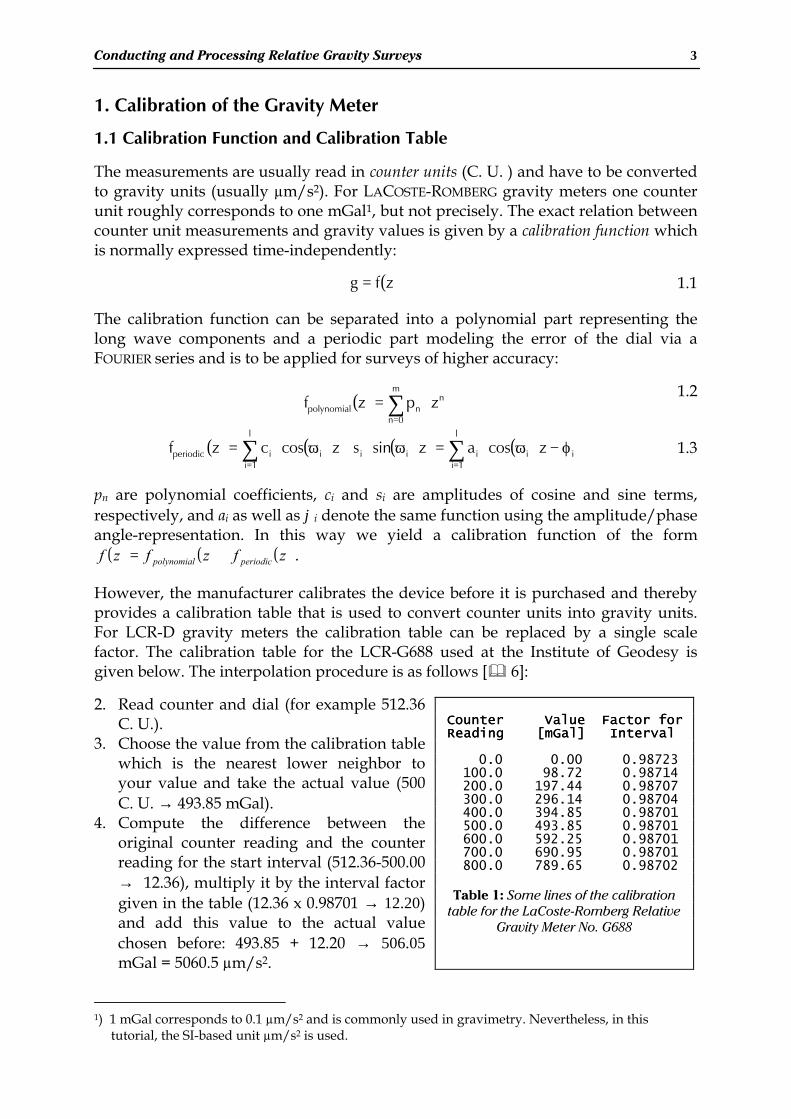
However, the manufacturer calibrates the device before it is purchased and therebyprovides a calibration table that is used to convert counter units into gravity units.For LCR-D gravity meters the calibration table can be replaced by a single scalefactor. The calibration table for the LCR-G688 used at the Institute of Geodesy isgiven below. The interpolation procedure is as follows [& 6]:

2. Read counter and dial (for example 512.36C. U.).

3. Choose the value from the calibration tablewhich is the nearest lower neighbor toyour value and take the actual value (500C. U. → 493.85 mGal).

4. Compute the difference between theoriginal counter reading and the counterreading for the start interval (512.36-500.00→ 12.36), multiply it by the interval factorgiven in the table (12.36 x 0.98701 → 12.20)and add this value to the actual valuechosen before: 493.85 + 12.20 → 506.05mGal = 5060.5 µm/s2.

1) 1 mGal corresponds to 0.1 µm/s2 and is commonly used in gravimetry. Nevertheless, in this tutorial, the SI-based unit µm/s2 is used.

Counter Value Factor forCounter Value Factor for Reading [ Reading [mGal] IntervalmGal] Interval

0.0 0.00 0.98723 100.0 98.72 0.98714 200.0 197.44 0.98707 300.0 296.14 0.98704 400.0 394.85 0.98701 500.0 493.85 0.98701 600.0 592.25 0.98701 700.0 690.95 0.98701 800.0 789.65 0.98702

Table 1: Some lines of the calibrationtable for the LaCoste-Romberg Relative

Gravity Meter No. G688


There might be, of course, variations over time that require a new calibration of thedevice. Moreover, for high precision measurements the manufacturer's calibrationinformation has to be improved or, at least, confirmed. In this way, we may considerthe calibration table as an approximated calibration function ( )f z0 that yieldsapproximately calibrated readings ( )~z f z= 0 . The main task of a new calibration isthe determination of the deviations from this approximate function. So, the calibrationfunction can be expressed - analogously to the first paragraph - as

( ) ( ) ( )f z f z f z= +0 ∆ where the last term ( ) ( ) ( )∆ ∆ ∆f z f z f zpolynomial periodic= + models thedeviations from the approximate function and is to be determined by the user. Ifhighest accuracy is not required, the periodic errors can be neglected (depends ongravity meter) and it may be sufficient to determine the linear error, i. e. higherdegree coefficients of the polynomial are neglected as well.

1.2 Determination of the Calibration Function

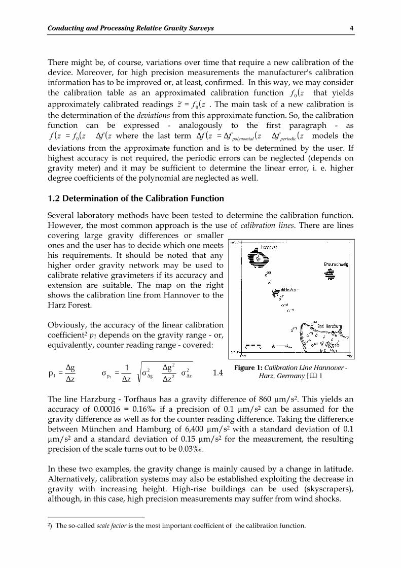
Several laboratory methods have been tested to determine the calibration function.However, the most common approach is the use of calibration lines. There are linescovering large gravity differences or smallerones and the user has to decide which one meetshis requirements. It should be noted that anyhigher order gravity network may be used tocalibrate relative gravimeters if its accuracy andextension are suitable. The map on the rightshows the calibration line from Hannover to theHarz Forest.

Obviously, the accuracy of the linear calibrationcoefficient2 p1 depends on the gravity range - or,equivalently, counter reading range - covered:

2z2

22

gp1 zg

z1

zg

p1 ∆∆ σ⋅

∆∆

+σ⋅∆

=σ⇒∆∆

= 1.4

The line Harzburg - Torfhaus has a gravity difference of 860 µm/s2. This yields anaccuracy of 0.00016 = 0.16‰ if a precision of 0.1 µm/s2 can be assumed for thegravity difference as well as for the counter reading difference. Taking the differencebetween München and Hamburg of 6,400 µm/s2 with a standard deviation of 0.1µm/s2 and a standard deviation of 0.15 µm/s2 for the measurement, the resultingprecision of the scale turns out to be 0.03‰.

In these two examples, the gravity change is mainly caused by a change in latitude.Alternatively, calibration systems may also be established exploiting the decrease ingravity with increasing height. High-rise buildings can be used (skyscrapers),although, in this case, high precision measurements may suffer from wind shocks.

2) The so-called scale factor is the most important coefficient of the calibration function.

Figure 1: Calibration Line Hannover -Harz, Germany [& 1


2. Planning and Conducting the Survey

2.1 Networks and Selection of Control Points

Gravity control points serve as a frame for subsequent detailed surveys. Thefollowing types of networks can be distinguished [& 3]:

• global gravity networks with station separations of a few 100 up to 1,000 km. Theyare the basic elements of gravity reference systems and are established ininternational cooperation;

• regional gravity networks with station separations of a few km to 100 km. Theyare established as national networks mostly in the form of a fundamental gravitynetwork with related densification networks;

• local gravity networks with station separations of a few 0.1 to 10 km. These aremostly established for geophysical or geodynamical purposes.

Some general aspects for the distribution and local selection of gravity control pointsmay be stated as follows:

• control point distribution as uniform as possible over the survey area, exceptionsmay be local geodynamic networks;

• local geological, seismic, and hydrological stability;• stable location for instrument setup (ground points in buildings, pillar, rock,

concrete floor), monumentation of the measurement point; it is expedient toutilize already existing markers of horizontal or vertical control points;

• establishment of 2 to 3 gravimetric eccenters (±0.01 to 0.1 µm/s2) for verificationof station integrity in fundamental gravity networks (eccenter separations a few100 m up to a few km; gravity differences smaller than 100 µm/s2);

• horizontal and vertical position determination relative to national controlnetworks.

2.2 Station Description

All gravity points are necessarily to be well documented, especially for retrievalpurposes. TORGE [& 3] gives the following advice as far as station documentation isconcerned:

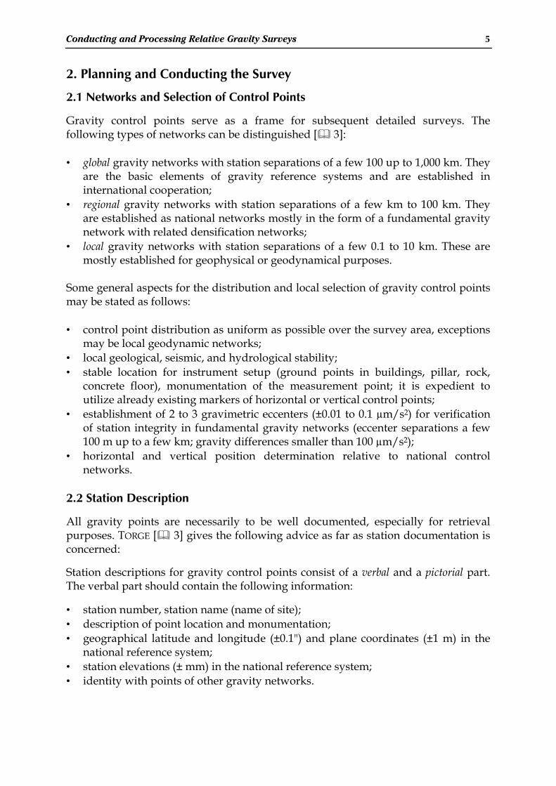
Station descriptions for gravity control points consist of a verbal and a pictorial part.The verbal part should contain the following information:

• station number, station name (name of site);• description of point location and monumentation;• geographical latitude and longitude (±0.1") and plane coordinates (±1 m) in the

national reference system;• station elevations (± mm) in the national reference system;• identity with points of other gravity networks.


It is useful to state an approximate gravity value (± µm/s2). For gravity basenetworks the address of the supervising organization should be included. Finally,station-specific information (earth tide parameters, local gravity gradient, geologicaland hydrological information) should be given if available.

The pictorial part should comprise:

• photographs of the measurement point and its dose proximity;• overview and in-survey sketches with data of local control measures;• extract of large scale map, 1:2,500 or similar (cadastral map, city map);• extract of topographic map, 1:50,000 or similar.

Photographs, survey sketches, and large scale map extract should focus particularlyon control of changes of the measurement station.

The requirements for station descriptions are less stringent for gravity points indensification networks and for regional and local surveys. A sketch of the in-surveyand a mark in a topographic map should always be completed.

Figure 2 shows two examples for extracts of station documentation as well assketches.

2.3 Preparation of the Survey

Prior to the survey of a network, the gravimeters have to undergo instrumentalinvestigations and calibrations. These include:

• laboratory tests with respect to dependencies on atmospheric pressure,temperature, magnetic field, shocks, and others;

• investigations of the drift behavior of spring gravimeters;• calibration of spring gravimeters in a calibration system with a range that exceeds

the gravity range of the survey area;• comparisons of different instruments by parallel surveys of the same points or the

same gravity differences, respectively.

These investigations lead to

• a-priori estimates of achievable measurement precision;• indications of systematic error sources which have to be taken into account by

modeling or by instrumental measures;


Figure 2: Two examples for gravity station descriptions and sketches. If the fixing of the gravity pointis not identical with the observation point like in the second example, this fact is to be clearly stressed(see marked entries!).

Photohere

Sketch

Height of gravitypoint fixing andthe actual point ofobservation


2.4 Accomplishment of the Survey

2.4.1 Survey Procedure and Drift Control

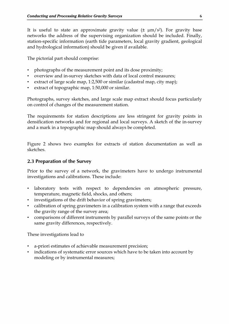
Sub-networks are surveyed with relative gravimeters whereby network stations areoften located on loops between stations of the fundamental network, and surveyed inlines using profile or step methods. A drift control should be planned in intervals of afew hours.

Figure 3: Typical drift determination methods arethe difference method (a) with three runs per line,the star method (b), the step method (c, stationwill be occupied three times) and the profilemethod (d, double occupation) [& 3]. The userhas to decide which one to choose with specialrespect to accuracy and efficiency. The differencemethod, for example, offers the advantage of highredundancy and, thus, one may expect a goodaccuracy, but it is economically very inefficient. Thestar method, in contrast, is more efficient. However,it might become inconvenient to return to thestarting point each time. The profile method offersdrift determination in forward-backward mannerand might be good overall compromise.

2.4.2 Azimuth Dependency

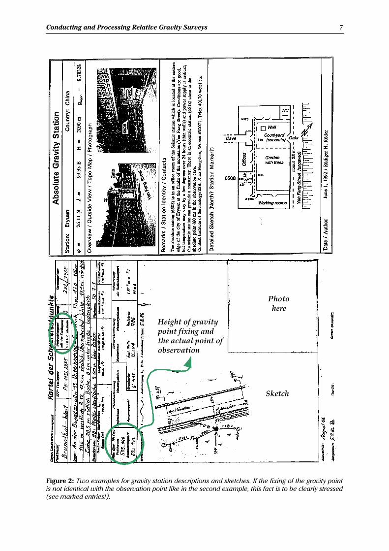
Spring gravimeters like LACOSTE-ROMBERG relativegravity meters (G and D) show an azimuth-dependency.This effect has to be eliminated by aligning thegravimeter to northward direction (use compass) or, ifnorth direction cannot be determined properly, by alwaysaligning the gravity meter with the same direction. Figure4 shows the azimuth-dependency for a LCR-G gravitymeter. The amplitude of the magnetic influence is about0.04 µm/s2.

Figure 4: Azimuth-dependentmagnetic effect on gravimeterreading of LCR-G298. [& 3]

2.4.3 Transport

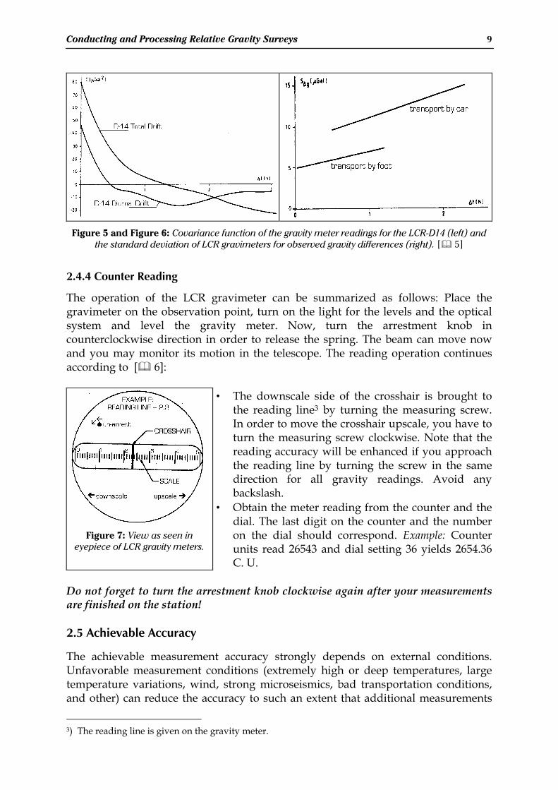
The covariance function of the counter readings might reveal a correlation due toseveral effects. One effect causing such correlation can be an incompletecompensation of the gravimeter drift, but, in practice, the drift is accounted for usingpolynomials or other models and the influence of the remainders does not cause anystrong correlation (see Figure 5). However, the conditions of transportation can have animpact on the variance and covariance: The standard deviation of the readingsincreases with time, see [& 5],

t0tl C2C2 ∆=∆∆ ⋅−⋅=σ 2.1

where Ci are the time-dependent values of the covariance function. The followingfigures show the covariance functions with respect to the gravimeter drift and theincrease in standard deviation for different kinds of transportation. Transportationby foot apparently yields most accurate results.


Figure 5 and Figure 6: Covariance function of the gravity meter readings for the LCR-D14 (left) andthe standard deviation of LCR gravimeters for observed gravity differences (right). [& 5]

2.4.4 Counter Reading

The operation of the LCR gravimeter can be summarized as follows: Place thegravimeter on the observation point, turn on the light for the levels and the opticalsystem and level the gravity meter. Now, turn the arrestment knob incounterclockwise direction in order to release the spring. The beam can move nowand you may monitor its motion in the telescope. The reading operation continuesaccording to [& 6]:

Figure 7: View as seen ineyepiece of LCR gravity meters.

• The downscale side of the crosshair is brought tothe reading line3 by turning the measuring screw.In order to move the crosshair upscale, you have toturn the measuring screw clockwise. Note that thereading accuracy will be enhanced if you approachthe reading line by turning the screw in the samedirection for all gravity readings. Avoid anybackslash.

• Obtain the meter reading from the counter and thedial. The last digit on the counter and the numberon the dial should correspond. Example: Counterunits read 26543 and dial setting 36 yields 2654.36C. U.

Do not forget to turn the arrestment knob clockwise again after your measurementsare finished on the station!

2.5 Achievable Accuracy

The achievable measurement accuracy strongly depends on external conditions.Unfavorable measurement conditions (extremely high or deep temperatures, largetemperature variations, wind, strong microseismics, bad transportation conditions,and other) can reduce the accuracy to such an extent that additional measurements

3) The reading line is given on the gravity meter.


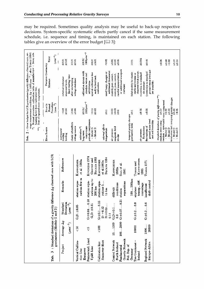
may be required. Sometimes quality analysis may be useful to back-up respectivedecisions. System-specific systematic effects partly cancel if the same measurementschedule, i.e. sequence and timing, is maintained on each station. The followingtables give an overview of the error budget [& 3]:


3. Pre-Processing of Data

Pre-processing of the data means computing the mean values per station, applyingcorrections and reductions and cleaning the data set. Some steps are explained here.

Instrumental Correction

First, the calibration correction is applied to the raw measurements as explained inchapter 1.

Height Reduction

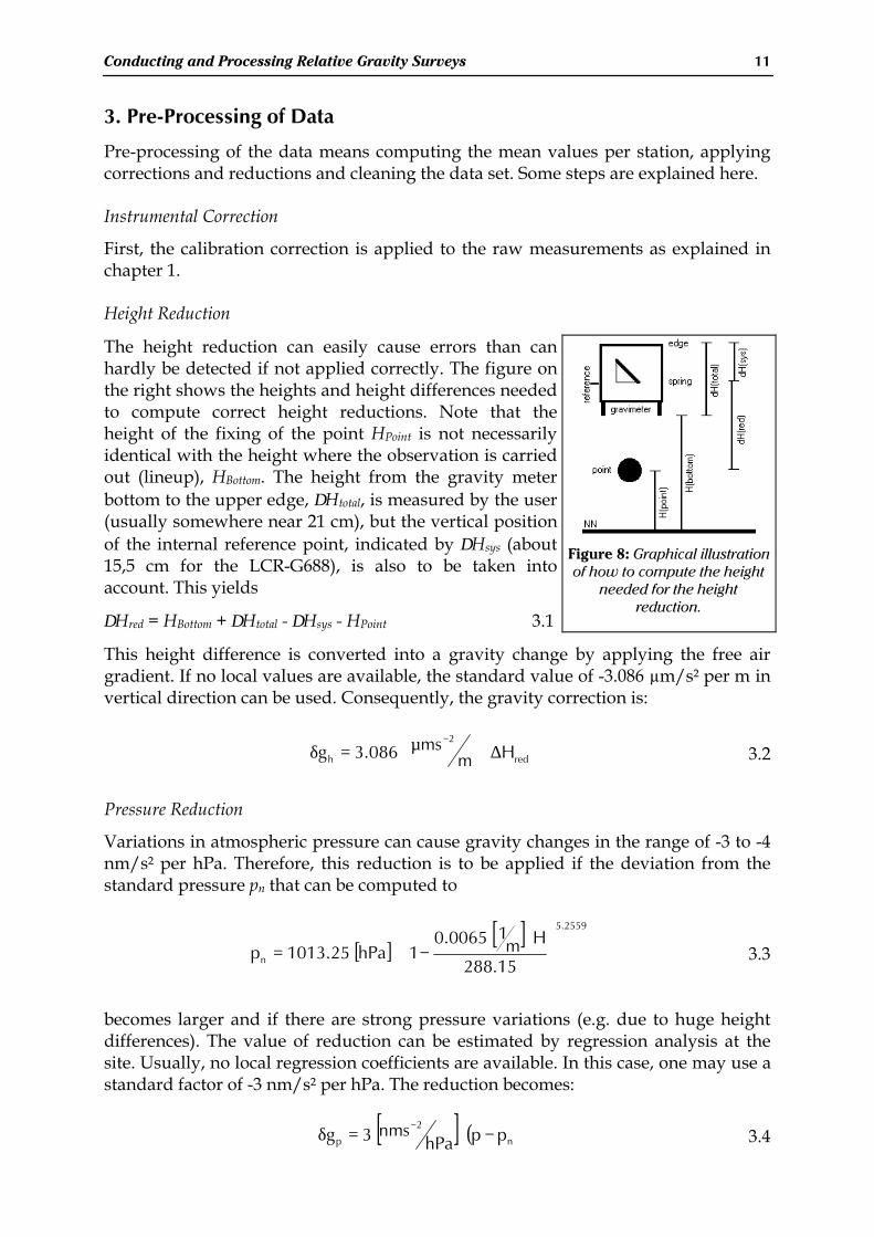
The height reduction can easily cause errors than canhardly be detected if not applied correctly. The figure onthe right shows the heights and height differences neededto compute correct height reductions. Note that theheight of the fixing of the point HPoint is not necessarilyidentical with the height where the observation is carriedout (lineup), HBottom. The height from the gravity meterbottom to the upper edge, ∆Htotal, is measured by the user(usually somewhere near 21 cm), but the vertical positionof the internal reference point, indicated by ∆Hsys (about15,5 cm for the LCR-G688), is also to be taken intoaccount. This yields

∆Hred = HBottom + ∆Htotal - ∆Hsys - HPoint 3.1

Figure 8: Graphical illustrationof how to compute the height

needed for the heightreduction.

This height difference is converted into a gravity change by applying the free airgradient. If no local values are available, the standard value of -3.086 µm/s² per m invertical direction can be used. Consequently, the gravity correction is:

red

2

h Hmms086.3g ∆⋅

µ=δ

−

3.2

Pressure Reduction

Variations in atmospheric pressure can cause gravity changes in the range of -3 to -4nm/s² per hPa. Therefore, this reduction is to be applied if the deviation from thestandard pressure pn that can be computed to

[ ][ ] 2559.5

n 15.288

Hm10065.0

1hPa25.1013p

⋅−⋅= 3.3

becomes larger and if there are strong pressure variations (e.g. due to huge heightdifferences). The value of reduction can be estimated by regression analysis at thesite. Usually, no local regression coefficients are available. In this case, one may use astandard factor of -3 nm/s² per hPa. The reduction becomes:

[ ] ( )n

2

p pphPanms3g −⋅=δ

−3.4


Tidal Reduction

Tidal reductions can be determined using several models. The expansion of the tidalpotential for the rigid earth by CARTWRIGHT-TAYLER-EDDEN was recommended by theIAG in 1971. This model is usually sufficient for field surveys. For highest precision,newer developments can be deployed. However, in this case it becomes moreimportant to use individual (local or regional) amplitude factors and phase angleshifts from observations at earth tide stations whereas in the normal case, agravimetric factor of 1.16 is a good choice.

Several potential developments have been conducted so far, for example:

Year No. of waves Developed by1921 378 DOODSON

1973 505 CARTWRIGHT-TAYLER-EDDEN

1985 665 BUELLESFELD

1987 1,200 TAMURA

1989 2,300 XI

1995 12,935 HARTMANN AND WENZEL

Table 2: Overview of tidal potential developments.

Ocean Loading Effects

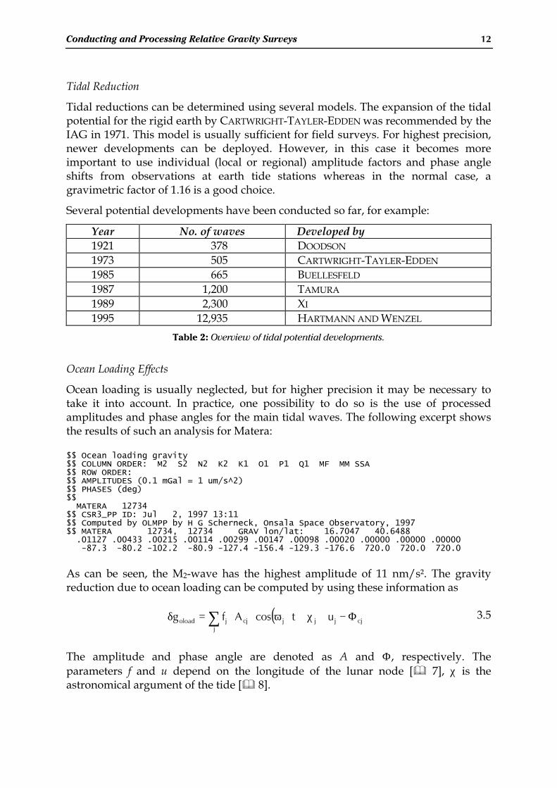
Ocean loading is usually neglected, but for higher precision it may be necessary totake it into account. In practice, one possibility to do so is the use of processedamplitudes and phase angles for the main tidal waves. The following excerpt showsthe results of such an analysis for Matera:

$$ Ocean loading gravity$$ COLUMN ORDER: M2 S2 N2 K2 K1 O1 P1 Q1 MF MM SSA$$ ROW ORDER:$$ AMPLITUDES (0.1 mGal = 1 um/s^2)$$ PHASES (deg)$$ MATERA 12734$$ CSR3_PP ID: Jul 2, 1997 13:11$$ Computed by OLMPP by H G Scherneck, Onsala Space Observatory, 1997$$ MATERA 12734, 12734 GRAV lon/lat: 16.7047 40.6488 .01127 .00433 .00215 .00114 .00299 .00147 .00098 .00020 .00000 .00000 .00000 -87.3 -80.2 -102.2 -80.9 -127.4 -156.4 -129.3 -176.6 720.0 720.0 720.0

As can be seen, the M2-wave has the highest amplitude of 11 nm/s². The gravityreduction due to ocean loading can be computed by using these information as

( )∑ Φ−+χ+⋅ω⋅⋅=δj

cjjjjcjjoload utcosAfg 3.5

The amplitude and phase angle are denoted as A and Φ, respectively. Theparameters f and u depend on the longitude of the lunar node [& 7], χ is theastronomical argument of the tide [& 8].


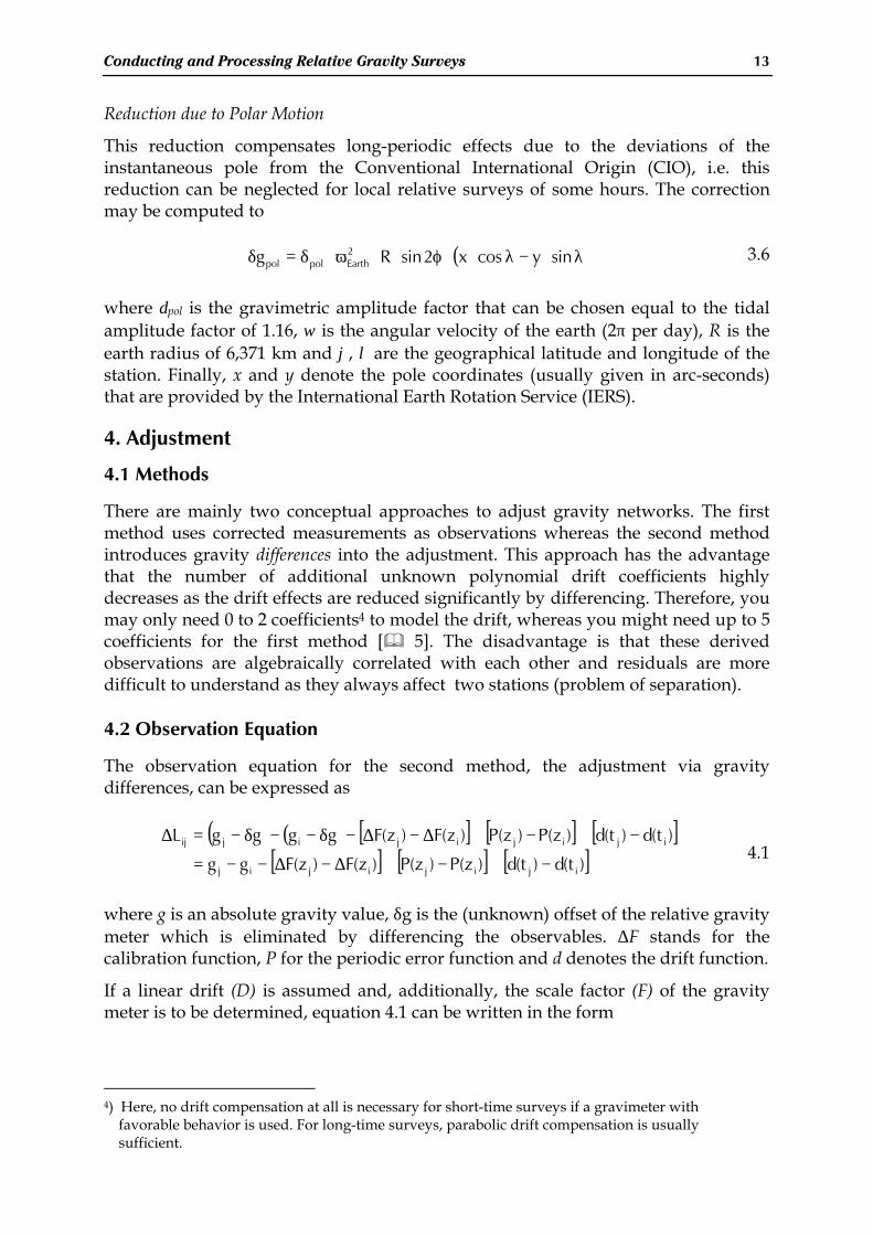
Reduction due to Polar Motion

This reduction compensates long-periodic effects due to the deviations of theinstantaneous pole from the Conventional International Origin (CIO), i.e. thisreduction can be neglected for local relative surveys of some hours. The correctionmay be computed to

( )λ⋅−λ⋅⋅ϕ⋅⋅ω⋅δ=δ sinycosx2sinRg 2Earthpolpol

3.6

where δpol is the gravimetric amplitude factor that can be chosen equal to the tidalamplitude factor of 1.16, ω is the angular velocity of the earth (2π per day), R is theearth radius of 6,371 km and ϕ, λ are the geographical latitude and longitude of thestation. Finally, x and y denote the pole coordinates (usually given in arc-seconds)that are provided by the International Earth Rotation Service (IERS).

4. Adjustment

4.1 Methods

There are mainly two conceptual approaches to adjust gravity networks. The firstmethod uses corrected measurements as observations whereas the second methodintroduces gravity differences into the adjustment. This approach has the advantagethat the number of additional unknown polynomial drift coefficients highlydecreases as the drift effects are reduced significantly by differencing. Therefore, youmay only need 0 to 2 coefficients4 to model the drift, whereas you might need up to 5coefficients for the first method [& 5]. The disadvantage is that these derivedobservations are algebraically correlated with each other and residuals are moredifficult to understand as they always affect two stations (problem of separation).

4.2 Observation Equation

The observation equation for the second method, the adjustment via gravitydifferences, can be expressed as

( ) ( ) [ ] [ ] [ ][ ] [ ] [ ])t(d)t(d)z(P)z(P)z(F)z(Fgg

)t(d)t(d)z(P)z(P)z(F)z(FggggL

ijijijij

ijijijijij

−+−+∆−∆−−=

−+−+∆−∆−δ−−δ−=∆4.1

where g is an absolute gravity value, δg is the (unknown) offset of the relative gravitymeter which is eliminated by differencing the observables. ∆F stands for thecalibration function, P for the periodic error function and d denotes the drift function.

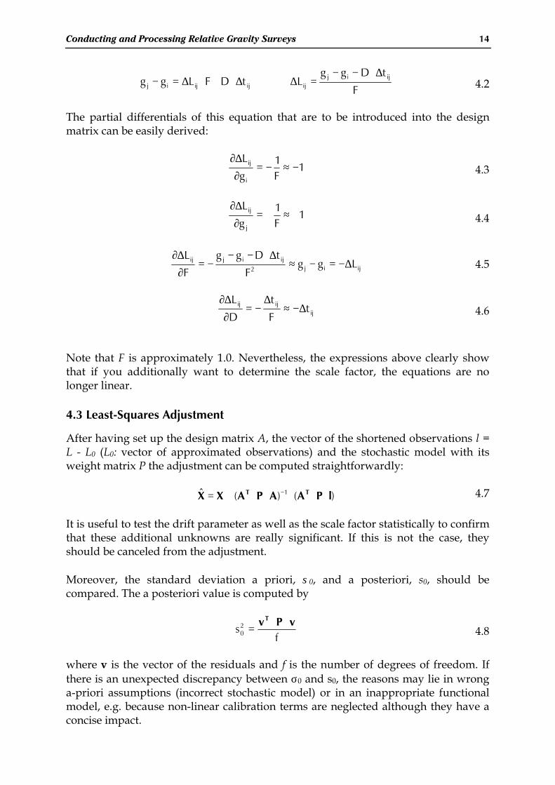
If a linear drift (D) is assumed and, additionally, the scale factor (F) of the gravitymeter is to be determined, equation 4.1 can be written in the form

4) Here, no drift compensation at all is necessary for short-time surveys if a gravimeter with favorable behavior is used. For long-time surveys, parabolic drift compensation is usually sufficient.


F

tDggLtDFLgg ijij

ijijijij

∆⋅−−=∆⇔∆⋅+⋅∆=− 4.2

The partial differentials of this equation that are to be introduced into the designmatrix can be easily derived:

1F1

g

L

i

ij −≈−=∂

∆∂4.3

1F1

g

L

j

ij +≈+=∂

∆∂4.4

ijij2ijijij Lgg

F

tDgg

F

L∆−=−≈

∆⋅−−−=

∂

∆∂4.5

ijijij t

F

t

D

L∆−≈

∆−=

∂

∆∂4.6

Note that F is approximately 1.0. Nevertheless, the expressions above clearly showthat if you additionally want to determine the scale factor, the equations are nolonger linear.

4.3 Least-Squares Adjustment

After having set up the design matrix A, the vector of the shortened observations l =L - L0 (L0: vector of approximated observations) and the stochastic model with itsweight matrix P the adjustment can be computed straightforwardly:

)()(ˆ 1 lPAAPAXX TT ⋅⋅⋅⋅⋅+= − 4.7

It is useful to test the drift parameter as well as the scale factor statistically to confirmthat these additional unknowns are really significant. If this is not the case, theyshould be canceled from the adjustment.

Moreover, the standard deviation a priori, σ0, and a posteriori, s0, should becompared. The a posteriori value is computed by

fs2

0vPvT ⋅⋅

= 4.8

where v is the vector of the residuals and f is the number of degrees of freedom. Ifthere is an unexpected discrepancy between σ0 and s0, the reasons may lie in wronga-priori assumptions (incorrect stochastic model) or in an inappropriate functionalmodel, e.g. because non-linear calibration terms are neglected although they have aconcise impact.


5. Bibliography

1. BECKER, MATTHIASAnalyse von hochpräzisen SchweremessungenDeutsche Geodätische Kommission bei der Bayerischen Akademie derWissenschaften, Reihe C, Dissertationen, Heft Nr. 294

2. KANNGIESER, E.Investigations of calibration functions, temperature and transportation effects atLaCoste-Romberg gravimetersin: Proc. Gen. Meeting of the I.A.G., Tokyo 1982, pp. 385-396, Special Issue Geod.Soc. of Japan, Tokyo 1982b

3. TORGE, WOLFGANGGravimetryWalter de Gruyter, Berlin – New York 1989

4. TORGE, WOLFGANGGeodäsieSammlung Göschen, de Gruyter, 1975

5. WENZEL, HANS-GEORGSchwerenetzein: H. PELZER (editor), Geodätische Netze in der Landes- undIngenieurvermessung II, K. Wittwer, Stuttgart 1985, pp. 457ff

6. Instruction Manual for LaCoste & Romberg, Inc. Model G Land Gravity MeterLaCoste & Romberg, Inc. Austin, Texas 78752, U. S. A.

7. DOODSON, A. T., 1928, The Analysis of Tidal Observations, Phil. Trans. Roy. Soc.Lond., 227, pp. 223-279

8. MCCARTHY, D., July 1996, IERS Conventions (1996), IERS Technical Note 21, U. S.Naval Observatory

rel grav tutorial

Documents

calibration function

gravity meter1

convertedto gravity

survey procedure

counter units

table of contents1

drift control

counter reading