Relation of Liquidity PreferenceRelation of Liquidity PreferenceFramework to Loanable FundsFramework to Loanable Funds

Keynes’s Major AssumptionKeynes’s Major Assumption

Two Categories of Assets in WealthTwo Categories of Assets in Wealth

MoneyMoney

BondsBonds

1.1. Thus:Thus: MMss + + BBss = Wealth = Wealth

2.2. Budget Constraint:Budget Constraint: BBdd + + MMdd = Wealth = Wealth

3.3. Therefore:Therefore: MMss + + BBss = = BBdd + + MMdd

4.4. Subtracting Subtracting MMdd and and BBss from both sides: from both sides:

MMss – – MMdd = = BBdd – – BBss

Money Market EquilibriumMoney Market Equilibrium

5.5. Occurs when Occurs when MMdd = = MMss

6.6. Then Then MMdd – – MMss = 0 which implies that = 0 which implies that BBdd – – BBss = 0, so that = 0, so that BBdd = = BBss and and bond market is also in equilibriumbond market is also in equilibrium

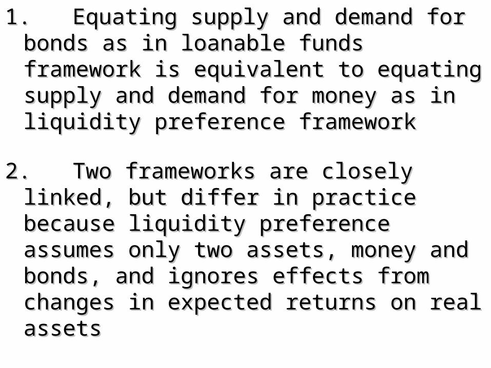
1.1.Equating supply and demand for bonds as in Equating supply and demand for bonds as in loanable funds framework is equivalent to loanable funds framework is equivalent to equating supply and demand for money as in equating supply and demand for money as in liquidity preference frameworkliquidity preference framework

2.2.Two frameworks are closely linked, but differ in Two frameworks are closely linked, but differ in practice because liquidity preference assumes practice because liquidity preference assumes only two assets, money and bonds, and ignores only two assets, money and bonds, and ignores effects from changes in expected returns on effects from changes in expected returns on real assetsreal assets

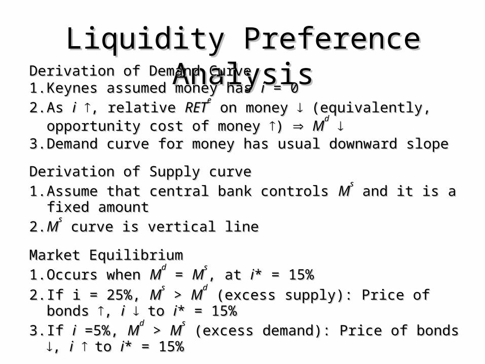
Liquidity Preference AnalysisLiquidity Preference AnalysisDerivation of Demand CurveDerivation of Demand Curve1.1. Keynes assumed money has Keynes assumed money has ii = 0 = 0

2.2. As As ii , relative , relative RETRETee on money on money (equivalently, opportunity cost of (equivalently, opportunity cost of

money money ) ) MMdd

3.3. Demand curve for money has usual downward slopeDemand curve for money has usual downward slope

Derivation of Supply curveDerivation of Supply curve

1.1. Assume that central bank controls Assume that central bank controls MMss and it is a fixed amount and it is a fixed amount

2.2. MMss curve is vertical line curve is vertical line

Market EquilibriumMarket Equilibrium

1.1. Occurs when Occurs when MMdd = = MM

ss, at , at ii* = 15%* = 15%

2.2. If i = 25%, If i = 25%, MMss > > MM

dd (excess supply): Price of bonds (excess supply): Price of bonds , , ii to to ii* = * =

15%15%

3.3. If If ii =5%, =5%, MMdd > > MM

ss (excess demand): Price of bonds (excess demand): Price of bonds , , ii to to ii* = * =

15%15%

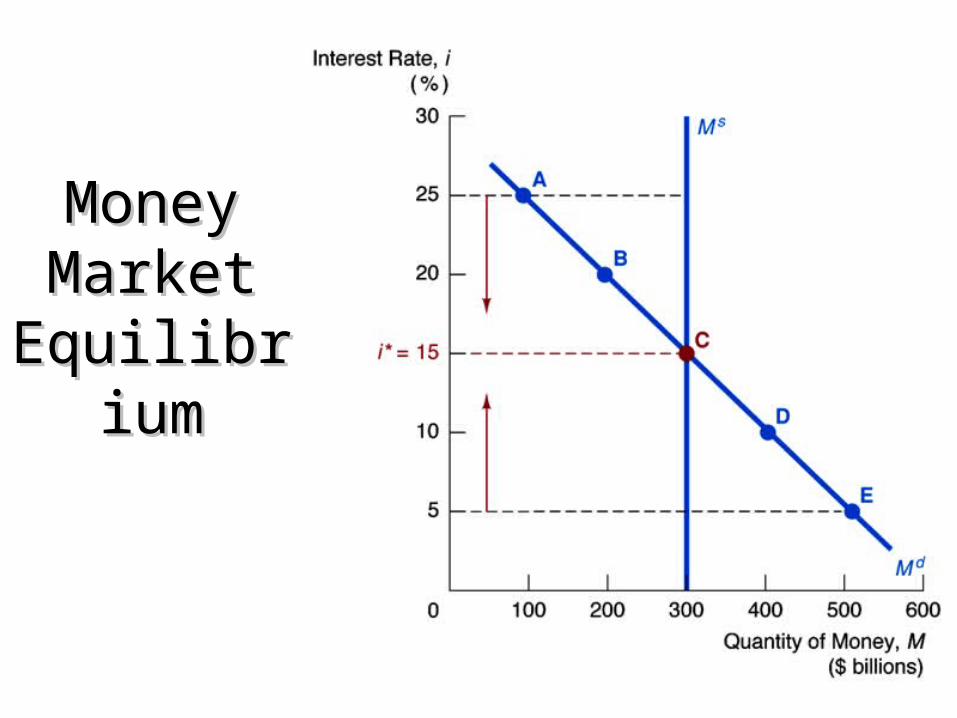
Money Money Market Market

EquilibriuEquilibriumm

Rise in Income or the Price LevelRise in Income or the Price Level

1.1. Income Income , , MMdd , , MMdd shifts out to rightshifts out to right

2.2. MMss unchanged unchanged33 ii* rises from * rises from ii11 to to ii22

Rise in Money SupplyRise in Money Supply

1.1. MMss , , MMss shifts out to shifts out to rightright

2.2. MMdd unchanged unchanged

3.3. ii* falls from * falls from ii11 to to ii

22

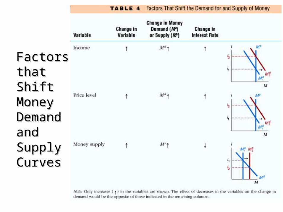
Factors Factors that Shift that Shift MoneyMoneyDemand Demand and and Supply Supply CurvesCurves

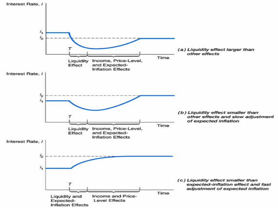
Money and Interest RatesMoney and Interest RatesEffects of money on interest ratesEffects of money on interest rates

1. Liquidity Effect1. Liquidity Effect

MMss , , MMss shifts right, shifts right, ii

2. Income Effect2. Income Effect

MMss , Income , Income , , MMdd , , MMdd shifts right, shifts right, ii

3. Price Level Effect3. Price Level Effect

MMss , Price level , Price level , , MMdd , , MMdd shifts right, shifts right, ii

4. Expected Inflation Effect4. Expected Inflation Effect

MMss , , ee , , BBdd , , BBss , Fisher effect, , Fisher effect, ii

Effect of higher rate of money growth on interest rates is Effect of higher rate of money growth on interest rates is ambiguousambiguous

1.1. Because income, price level and expected inflation effects Because income, price level and expected inflation effects workwork

in opposite direction of liquidity effectin opposite direction of liquidity effect

Evidence on Money Growth Evidence on Money Growth and Interest Ratesand Interest Rates

Risk Structure of Long Bonds in Risk Structure of Long Bonds in the United Statesthe United States

Increase in Default Risk on Increase in Default Risk on Corporate BondsCorporate Bonds

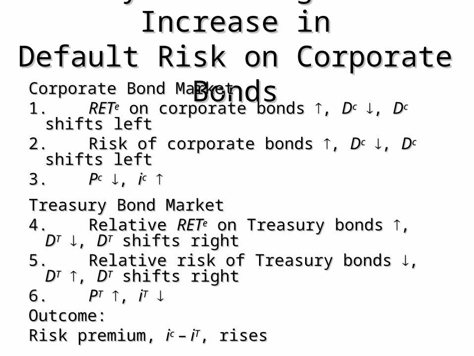
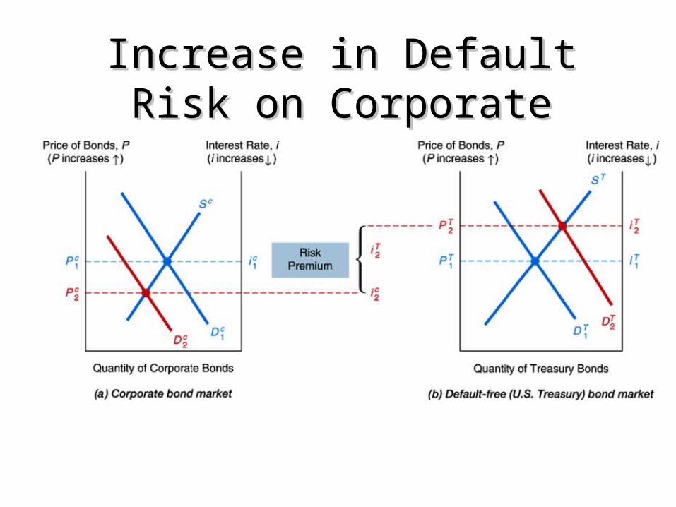
Analysis of Figure 2: Increase inAnalysis of Figure 2: Increase inDefault Risk on Corporate BondsDefault Risk on Corporate BondsCorporate Bond MarketCorporate Bond Market1.1. RETRETee on corporate bonds on corporate bonds , , DDcc , , DDcc shifts left shifts left2.2. Risk of corporate bonds Risk of corporate bonds , , DDcc , , DDcc shifts left shifts left3.3. PPcc , , iicc

Treasury Bond MarketTreasury Bond Market4.4. Relative Relative RETRETee on Treasury bonds on Treasury bonds , , DDTT , , DDTT

shifts rightshifts right5.5. Relative risk of Treasury bonds Relative risk of Treasury bonds , , DDTT , , DDTT shifts shifts

rightright6.6. PPTT , , iiTT Outcome:Outcome:Risk premium, Risk premium, iicc – i – iTT, rises, rises

Bond RatingsBond Ratings

Corporate Bonds Become Less Corporate Bonds Become Less LiquidLiquid

Corporate Bond MarketCorporate Bond Market

1.1. Less liquid corporate bonds Less liquid corporate bonds DDcc , , DDcc shifts left shifts left

2.2. PPcc , , iicc

Treasury Bond MarketTreasury Bond Market1.1. Relatively more liquid Treasury bonds, Relatively more liquid Treasury bonds, DDTT , , DDTT shifts shifts

rightright

2.2. PPTT , , iiTT Outcome:Outcome:

Risk premium, Risk premium, iicc – i – iTT, rises, rises

Risk premium reflects not only corporate bonds’ default Risk premium reflects not only corporate bonds’ default risk, but also lower liquidityrisk, but also lower liquidity

Tax Advantages of Municipal Tax Advantages of Municipal BondsBonds

Analysis of Figure 3: Tax Analysis of Figure 3: Tax Advantages Advantages

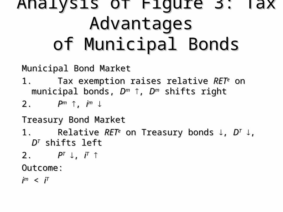
of Municipal Bondsof Municipal BondsMunicipal Bond MarketMunicipal Bond Market

1.1. Tax exemption raises relative Tax exemption raises relative RETRETee on municipal on municipal bonds, bonds, DDmm , , DDmm shifts right shifts right

2.2. PPmm , , iimm

Treasury Bond MarketTreasury Bond Market

1.1. Relative Relative RETRETee on Treasury bonds on Treasury bonds , , DDTT , , DDTT shifts left shifts left

2.2. PPTT , , iiTT Outcome:Outcome:

iimm < < iiTT

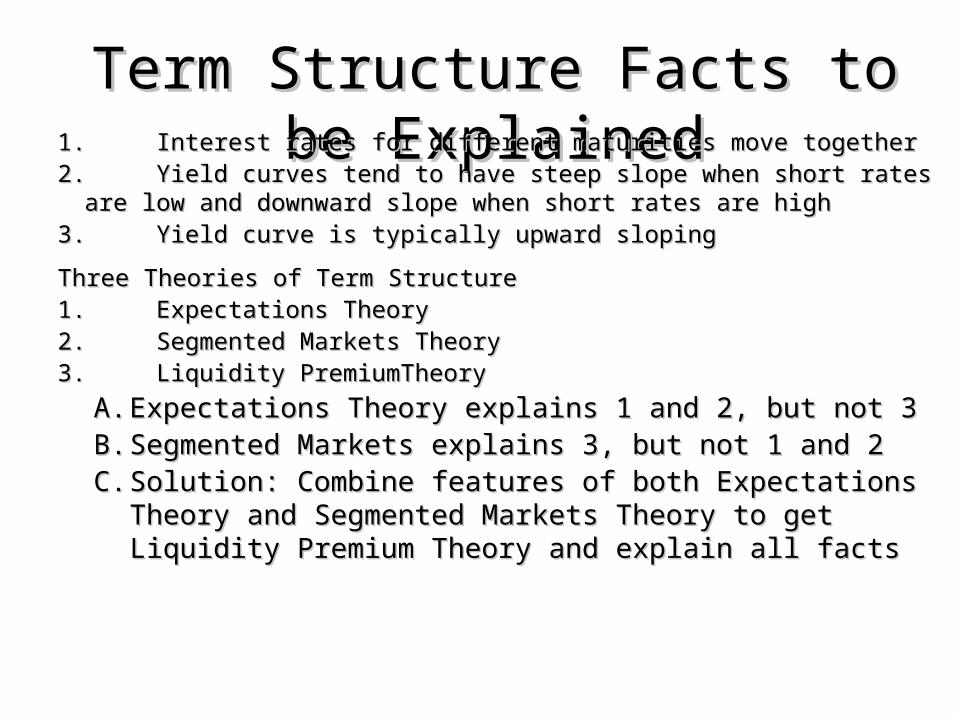
Term Structure Facts to be Term Structure Facts to be ExplainedExplained1.1. Interest rates for different maturities move togetherInterest rates for different maturities move together

2.2. Yield curves tend to have steep slope when short rates are low Yield curves tend to have steep slope when short rates are low and downward slope when short rates are highand downward slope when short rates are high

3.3. Yield curve is typically upward slopingYield curve is typically upward sloping

Three Theories of Term StructureThree Theories of Term Structure1.1. Expectations TheoryExpectations Theory2.2. Segmented Markets TheorySegmented Markets Theory3.3. Liquidity PremiumTheoryLiquidity PremiumTheory

A.A. Expectations Theory explains 1 and 2, but not 3Expectations Theory explains 1 and 2, but not 3B.B. Segmented Markets explains 3, but not 1 and 2Segmented Markets explains 3, but not 1 and 2C.C. Solution: Combine features of both Expectations Solution: Combine features of both Expectations

Theory and Segmented Markets Theory to get Theory and Segmented Markets Theory to get Liquidity Premium Theory and explain all factsLiquidity Premium Theory and explain all facts

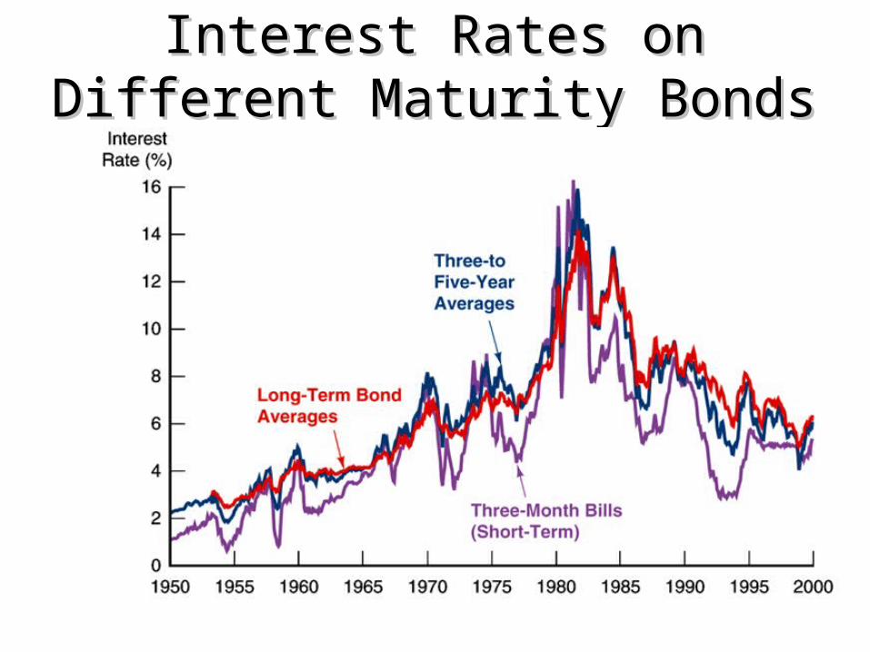
Interest Rates on Different Maturity Interest Rates on Different Maturity Bonds Move TogetherBonds Move Together

Yield CurvesYield Curves

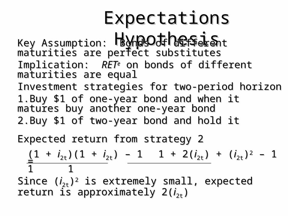
Expectations HypothesisExpectations HypothesisKey Assumption:Key Assumption: Bonds of different maturities are Bonds of different maturities are perfect substitutesperfect substitutesImplication:Implication: RETRETee on bonds of different maturities are on bonds of different maturities are equalequalInvestment strategies for two-period horizonInvestment strategies for two-period horizon1.1. Buy $1 of one-year bond and when it matures buy Buy $1 of one-year bond and when it matures buy another another one-year bondone-year bond2.2. Buy $1 of two-year bond and hold itBuy $1 of two-year bond and hold it

Expected return from strategy 2Expected return from strategy 2

(1 + (1 + ii2t2t)(1 + )(1 + ii2t2t) – 1) – 1 1 + 2(1 + 2(ii2t2t) + () + (ii2t2t))22 – 1 – 1==

11 11Since (Since (ii2t2t))22 is extremely small, expected return is is extremely small, expected return is approximately 2(approximately 2(ii2t2t))

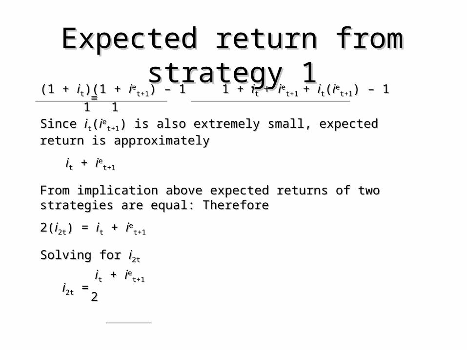
Expected return from Expected return from strategy 1strategy 1

(1 + (1 + iitt)(1 + )(1 + iieet+1t+1) – 1) – 1 1 + 1 + iit t + + iieet+1 t+1 + + iitt((iiee

t+1t+1) – 1) – 1==

1 1 11Since Since iitt((iie

et+1t+1) is also extremely small, expected return is ) is also extremely small, expected return is

approximatelyapproximately

iitt + + iieet+1t+1

From implication above expected returns of two strategies are equal: From implication above expected returns of two strategies are equal: ThereforeTherefore

2(2(ii2t2t) = ) = iitt + + iieet+1t+1

Solving for Solving for ii2t 2t

iitt + + iieet+1t+1

ii2t2t = = 22

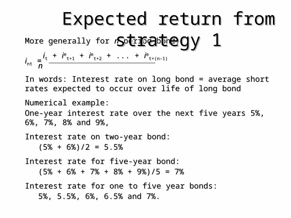
More generally for More generally for nn-period bond:-period bond:

iitt + + iieet+1t+1 + + iieet+2t+2 + ... + + ... + iieet+(n–1)t+(n–1)iintnt = = nn

In words: Interest rate on long bond = average short rates expected In words: Interest rate on long bond = average short rates expected to occur over life of long bondto occur over life of long bond

Numerical example:Numerical example:One-year interest rate over the next five years 5%, 6%, 7%, 8% One-year interest rate over the next five years 5%, 6%, 7%, 8% and 9%,and 9%,

Interest rate on two-year bond:Interest rate on two-year bond:(5% + 6%)/2 = 5.5%(5% + 6%)/2 = 5.5%

Interest rate for five-year bond:Interest rate for five-year bond:(5% + 6% + 7% + 8% + 9%)/5 = 7%(5% + 6% + 7% + 8% + 9%)/5 = 7%

Interest rate for one to five year bonds:Interest rate for one to five year bonds:5%, 5.5%, 6%, 6.5% and 7%.5%, 5.5%, 6%, 6.5% and 7%.

Expected return from Expected return from strategy 1strategy 1

Expectations Hypothesis and Term Structure FactsExpectations Hypothesis and Term Structure Facts

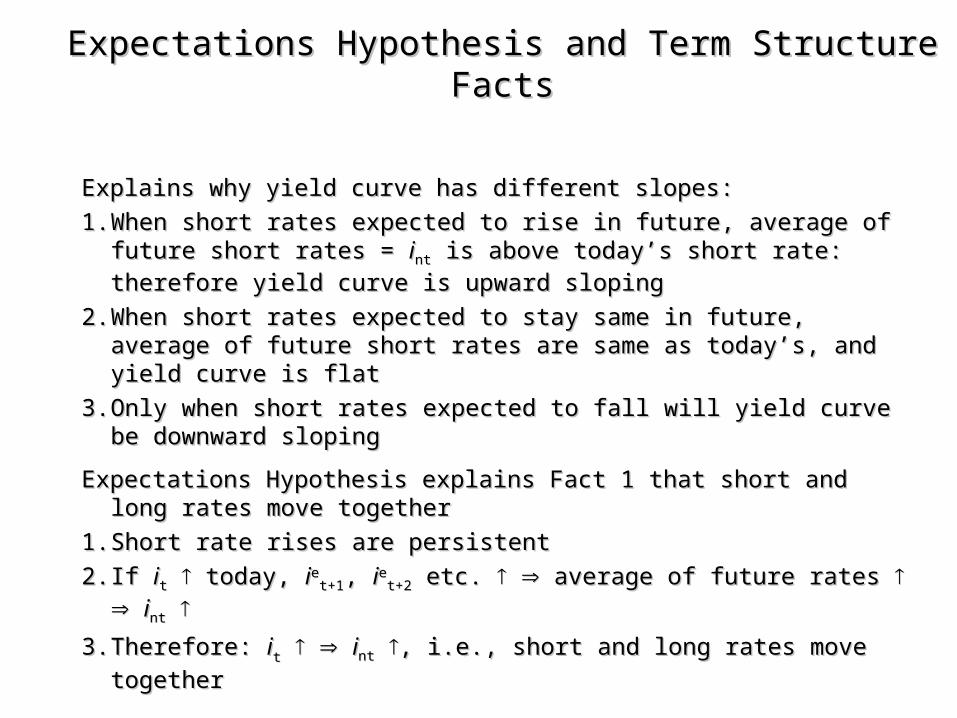
Explains why yield curve has different slopes:Explains why yield curve has different slopes:

1.1. When short rates expected to rise in future, average of future When short rates expected to rise in future, average of future short rates = short rates = iintnt is above today’s short rate: therefore yield is above today’s short rate: therefore yield

curve is upward slopingcurve is upward sloping

2.2. When short rates expected to stay same in future, average of When short rates expected to stay same in future, average of future short rates are same as today’s, and yield curve is flatfuture short rates are same as today’s, and yield curve is flat

3.3. Only when short rates expected to fall will yield curve be Only when short rates expected to fall will yield curve be downward slopingdownward sloping

Expectations Hypothesis explains Fact 1 that short and long Expectations Hypothesis explains Fact 1 that short and long rates move togetherrates move together

1.1. Short rate rises are persistentShort rate rises are persistent

2.2. If If iitt today, today, iieet+1t+1, , iieet+2t+2 etc. etc. average of future rates average of future rates iintnt

3.3. Therefore: Therefore: iitt iintnt , i.e., short and long rates move together, i.e., short and long rates move together

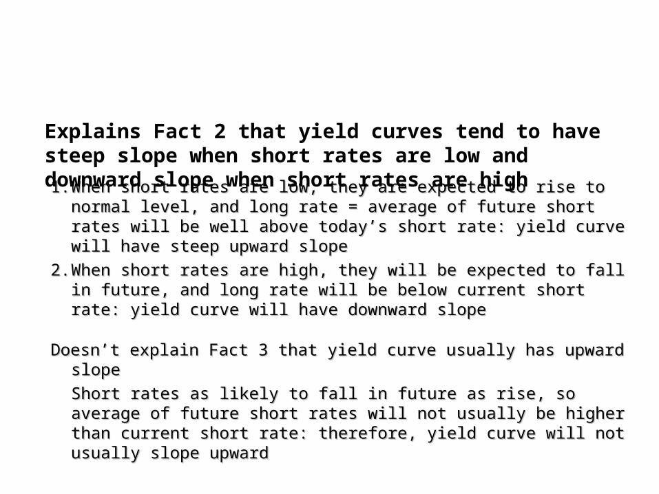
1.1. When short rates are low, they are expected to rise to normal When short rates are low, they are expected to rise to normal level, and long rate = average of future short rates will be well level, and long rate = average of future short rates will be well above today’s short rate: yield curve will have steep upward above today’s short rate: yield curve will have steep upward slopeslope

2.2. When short rates are high, they will be expected to fall in When short rates are high, they will be expected to fall in future, and long rate will be below current short rate: yield future, and long rate will be below current short rate: yield curve will have downward slopecurve will have downward slope

Doesn’t explain Fact 3 that yield curve usually has upward slopeDoesn’t explain Fact 3 that yield curve usually has upward slope

Short rates as likely to fall in future as rise, so average of Short rates as likely to fall in future as rise, so average of future short rates will not usually be higher than current short future short rates will not usually be higher than current short rate: therefore, yield curve will not usually slope upwardrate: therefore, yield curve will not usually slope upward

Explains Fact 2 that yield curves tend to have steep slope when short rates are low and downward slope when short rates are high

Segmented Markets TheorySegmented Markets Theory

Key Assumption: Key Assumption: Bonds of different maturities are not Bonds of different maturities are not substitutes at allsubstitutes at all

Implication: Implication: Markets are completely segmented: Markets are completely segmented: interest rate at each maturity determined separatelyinterest rate at each maturity determined separately

Explains Fact 3 that yield curve is usually upward Explains Fact 3 that yield curve is usually upward slopingsloping

People typically prefer short holding periods and thus People typically prefer short holding periods and thus have higher demand for short-term bonds, which have have higher demand for short-term bonds, which have higher price and lower interest rates than long bondshigher price and lower interest rates than long bonds

Does not explain Fact 1 or Fact 2 because assumes Does not explain Fact 1 or Fact 2 because assumes long and short rates determined independentlylong and short rates determined independently

Liquidity Premium TheoryLiquidity Premium Theory

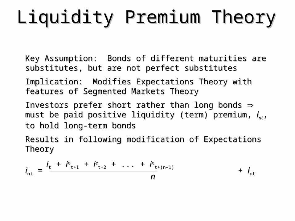
Key Assumption:Key Assumption: Bonds of different maturities are Bonds of different maturities are substitutes, but are not perfect substitutessubstitutes, but are not perfect substitutes

Implication:Implication: Modifies Expectations Theory with features of Modifies Expectations Theory with features of Segmented Markets TheorySegmented Markets Theory

Investors prefer short rather than long bonds Investors prefer short rather than long bonds must be must be paid positive liquidity (term) premium, paid positive liquidity (term) premium, llntnt, to hold long-term , to hold long-term

bondsbonds

Results in following modification of Expectations TheoryResults in following modification of Expectations Theory

iitt + + iieet+1t+1 + + iieet+2t+2 + ... + + ... + iieet+(n–1)t+(n–1)iintnt = = + + llntnt nn

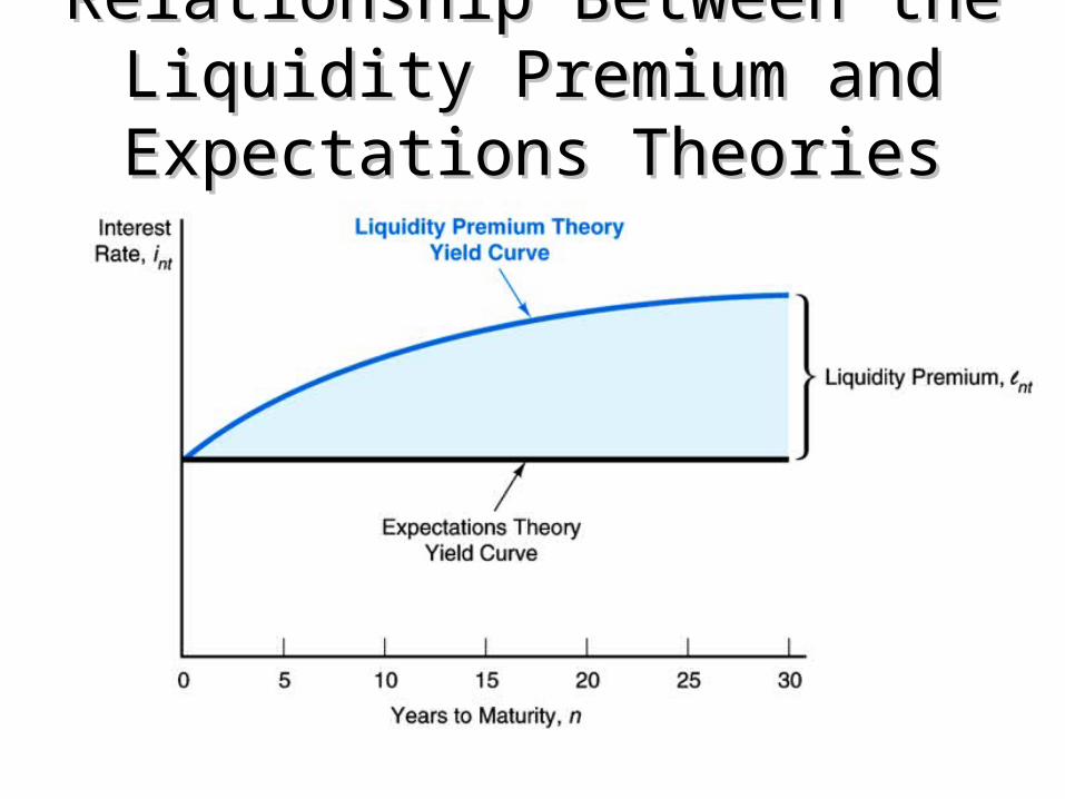
Relationship Between the Liquidity Relationship Between the Liquidity Premium and Expectations Premium and Expectations

TheoriesTheories

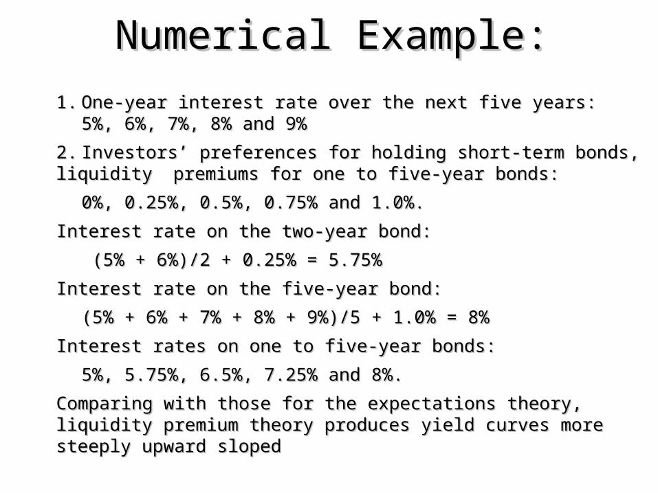
Numerical Example:Numerical Example:

1.1. One-year interest rate over the next five years:One-year interest rate over the next five years:5%, 6%, 7%, 8% and 9%5%, 6%, 7%, 8% and 9%

2.2. Investors’ preferences for holding short-term bonds, liquidity Investors’ preferences for holding short-term bonds, liquidity premiums for one to five-year bonds:premiums for one to five-year bonds:

0%, 0.25%, 0.5%, 0.75% and 1.0%.0%, 0.25%, 0.5%, 0.75% and 1.0%.

Interest rate on the two-year bond:Interest rate on the two-year bond:

(5% + 6%)/2 + 0.25% = 5.75%(5% + 6%)/2 + 0.25% = 5.75%

Interest rate on the five-year bond:Interest rate on the five-year bond:

(5% + 6% + 7% + 8% + 9%)/5 + 1.0% = 8%(5% + 6% + 7% + 8% + 9%)/5 + 1.0% = 8%

Interest rates on one to five-year bonds:Interest rates on one to five-year bonds:

5%, 5.75%, 6.5%, 7.25% and 8%.5%, 5.75%, 6.5%, 7.25% and 8%.

Comparing with those for the expectations theory, liquidity premium Comparing with those for the expectations theory, liquidity premium theory produces yield curves more steeply upward slopedtheory produces yield curves more steeply upward sloped

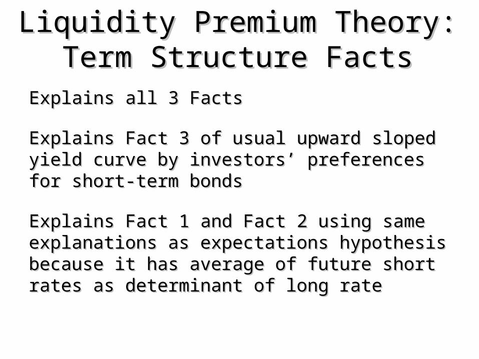
Liquidity Premium Theory: Term Liquidity Premium Theory: Term Structure FactsStructure Facts

Explains all 3 FactsExplains all 3 Facts

Explains Fact 3 of usual upward sloped yield Explains Fact 3 of usual upward sloped yield curve by investors’ preferences for short-term curve by investors’ preferences for short-term bondsbonds

Explains Fact 1 and Fact 2 using same Explains Fact 1 and Fact 2 using same explanations as expectations hypothesis explanations as expectations hypothesis because it has average of future short rates because it has average of future short rates as determinant of long rateas determinant of long rate

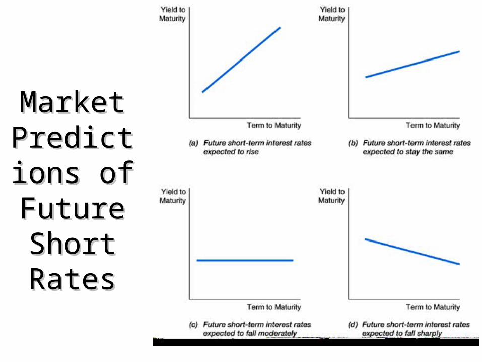
Market Market PredictionPrediction

s of s of Future Future Short Short RatesRates