Relational Foundations For Functorial Data Migration ∗

David I. Spivak, Ryan Wisnesky †Massachusetts Institute of Technology{dspivak, wisnesky}@math.mit.edu

July 28, 2015Abstract

We study the data transformation capabilities associated with schemas that are presented by directed multi-graphs and path equations. Unlike most approaches which treat graph-based schemas as abbreviations for rela-tional schemas, we treat graph-based schemas as categories. A schema S is a finitely-presented category, and thecollection of all S-instances forms a category, S–Inst. A functor F between schemas S and T , which can be gener-ated from a visual mapping between graphs, induces three adjoint data migration functors, ΣF : S–Inst → T –Inst,ΠF : S–Inst → T –Inst, and ∆F : T –Inst → S–Inst. We present an algebraic query language FQL based on thesefunctors, prove that FQL is closed under composition, prove that FQL can be implemented with the select-project-product-union relational algebra (SPCU) extended with a key-generation operation, and prove that SPCU can beimplemented with FQL.

1 Introduction

In this paper we describe how to implement functorialdata migration [16] using relational algebra, and viceversa. In the functorial data model [16], a databaseschema is a finitely-presented category (a directed multi-graph with path equations [4]), and a database instanceon a schema S is a functor from S to the category of sets,Set. The database instances on a schema S constitutea category, denoted S–Inst, and a functor F betweenschemas S and T induces three data migration functors:∆F : T–Inst→ S–Inst, defined as ∆F (I) := F ◦ I, andits left and right adjoints ΣF : S–Inst → T–Inst andΠF : S–Inst→ T–Inst, respectively. We define a func-torial query language, FQL, in which every query de-notes a data migration functor, prove that FQL is closedunder composition, and define a translation from FQLto the select-project-product-union (SPCU) relationalalgebra extended with an operation for creating globallyunique IDs (GUIDs)1. In addition, we describe how toimplement the SPCU relational algebra with FQL.

Our primary motivation for this work is to use SQLas a practical deployment platform for the functorialdata model. Using the results of this paper we haveimplemented a SQL compiler for FQL, and a (partial)translator from SQL to FQL, as part of a visual schemamapping tool available at categoricaldata.net/fql.html.We are interested in the functorial data model be-cause we believe its category-theoretic underpinningsprovide a better mathematical foundation for informa-

tion integration than the relational model. For ex-ample, many practical “relational” systems (includingSQL-based RDBMSs) are not actually relational, butare based on bags and unique row IDs—like the functo-rial data model. Numerous advantages of the functorialdata model are described in [16] and [8].

1.1 Related Work

Although category presentations—directed multi-graphs with path equivalence constraints—are a com-mon notation for schemas [5], prior work rarely treatssuch schemas categorically [8]. Instead, most priorwork treats such schemas as abbreviations for relationalschemas. For example, in Clio [10], users draw linesconnecting related elements between two schemas-as-graphs and Clio generates a relational query (seman-tically similar to our Σ) that implements the user’sintended data transformation. Behind the scenes, theuser’s correspondence is translated into a formula inthe relational language of second-order tuple generatingdependencies, from which a query is generated [7].

In many ways, our work is an extension and improve-ment of Rosebrugh et al’s initial work on understand-ing category presentations as database schemas [8]. Inthat work, the authors identify the Σ and Π data mi-gration functors, but they do not identify ∆ as theiradjoint. Moreover, they do not implement Σ and Πusing relational algebra, and they do not formalize aquery language or investigate the behavior of Σ and Π

∗Extended version of the DBPL 2015 paper.†Work funded by ONR grants N000141010841 and N000141310260.1An operation to create IDs is required because functorial data migration can create constants not contained in input instances.

1

arX

iv:1

212.

5303

v7 [

cs.D

B]

24

Jul 2

015

with respect to composition; neither do they consider“attributes”. Our mathematical development divergesfrom their subsequent work on “sketches” [13], in whichsome or all of ∆, Σ, and Π data migration functors mayno longer exist.

Category-theoretic techniques were instrumentalin the development of the nested relational datamodel [17]. However, we do not believe that the func-torial data model and the nested relational model areclosely connected. The functorial data model is moreclosely related to work on categorical logic and typetheory, where operations similar to Σ,Π, and ∆ oftenappear under the slogan that “quantification is adjointto substitution” [12].

1.2 Contributions and OutlineWe make the following contributions:

1. The naive functorial data model [8], as sketchedabove, is not quite appropriate for many practi-cal information management tasks. Intuitively,this is because many categorical constructions areonly defined up to isomorphism; at a practicallevel, this means that every instance must containonly meaningless IDs [16]. The idea to extendthe functorial data model with “attributes” tocapture meaningful concrete data such as stringsand integers was originally developed in [16]. Inthis paper, we refine that notion of attribute sothat our schemas become special kinds of entity-relationship (ER) diagrams (those in “categoricalnormal form”), and our instances can be repre-sented as relational tables that conform to suchER diagrams. (Sections 2 and 3)

2. We define an algebraic query language FQL inwhich every query denotes a data migration func-tor in the above extended sense. We show thatFQL queries are closed under composition, andhow every query in FQL can be described asa triplet of graph correspondences (similar toschema mappings [10]). Determining whether atriplet of arbitrary graph correspondences is anFQL query is semi-decidable. (Section 4)

3. We provide a translation of FQL into the SPCUrelational algebra of selection, projection, carte-sian product, and union extended with a globallyunique ID generator that constructs N + 1-arytables from N -ary tables by adding a globallyunique ID to each row. This allows us to generateSQL programs that implement FQL. A corollary isthat materializing result instances of FQL querieshas polynomial time data complexity. (Section 5)

4. We show that every SPCU query under bag se-mantics is expressible in FQL, and how to extendFQL with an operation allowing it to capture ev-ery SPCU query under set semantics. (Section 6)

For every schema S, the category S–Inst is atopos [4]. Hence, the functorial data model admits otheroperations on instances besides the functorial data mi-gration operations that are the focus of this paper. Weconclude with a discussion of which of these operationscan be implemented in SPCU+keygen (Section 7).

2 Categorical DataIn this section we define the original signatures and in-stances of [16], as well as “typed signatures” and “typedinstances”, which are our extension of [16] to attributes.The basic idea is that signatures are stylized ER di-agrams that denote categories, and our database in-stances can be represented as instances of such ER di-agrams, and vice versa (up to natural isomorphism).From this point on, we will distinguish between a sig-nature, which is a finite presentation of a category, anda schema, which is the category a signature denotes.

2.1 SignaturesThe functorial data model [16] uses directed labeledmulti-graphs and path equalities for signatures. A pathp is defined inductively as:

p ::= node | p.edge

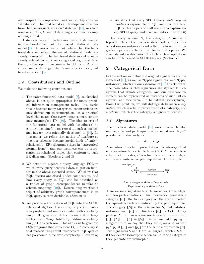
A signature S is a finite presentation of a category. Thatis, a signature S is a triple S := (N,E,C) where N isa finite set of nodes, E is a finite set of directed edges,and C is a finite set of path equations. For example:

Emp•

worksIn //

manager��

Dept•

secretaryoo

Emp.manager.worksIn = Emp.worksInDept.secretary.worksIn = Dept

Here we see a signature S with two nodes, three edges,and two path equations. This information generates acategory ~S�: the free category on the graph, modulothe equivalence relation induced by the path equations.The category ~S� is the schema for S, and databaseinstances over ~S� are functors ~S� → Set. Everypath p : X → Y in a signature S denotes a morphism~p� : ~X� → ~Y � in ~S�. Given two paths p1, p2 ina signature S, we say that they are equivalent, writtenp1 � p2, if ~p1� and ~p2� are the same morphism in ~S�.Two signatures S and T are isomorphic, written S � T ,if they denote isomorphic schemas, i.e. if the categoriesthey generate are isomorphic.

2

2.2 Cyclic SignaturesIf a signature contains a loop, it may or may not de-note a category with infinitely many morphisms. Hence,some constructions over signatures may not be com-putable. Testing if two paths in a signature are equiv-alent is known as the word problem for categories. Theword problem can be semi-decided using the “comple-tion without failure” extension [3] of the Knuth-Bendixalgorithm. This algorithm first attempts to construct astrongly normalizing re-write system based on the pathequalities; if it succeeds, it yields a linear time deci-sion procedure for the word problem [11]. If a signaturedenotes a finite category, the Carmody-Walters algo-rithm [6] will compute its denotation. This algorithmcomputes left Kan extensions and can be used for manypurposes in computational category theory [8].

2.3 InstancesLet S be a signature. A S-instance is a functor from~S� to the category of sets. We will represent instancesas relational tables using the following binary format:

• To each node N corresponds an “identity” or “en-tity” table named N , a reflexive table with tuplesof the form (x, x). We can specify this using first-order logic:

∀xy.N(x, y)⇒ x = y. (1)

The entries in these tables are called IDs or keys,and for the purposes of this paper we require themto be globally unique. We call this the globallyunique key assumption. Note that it is possible touse unary tables instead of binary tables, but wehave found the uniform binary format to be sim-pler when manipulating instances using e.g., SQL.

• To each edge e : N1 → N2 corresponds a “link”table e between identity tables N1 and N2. Theaxioms below say that every edge e : N1 → N2designates a total function N1 → N2:

∀xy. e(x, y)⇒ N1(x, x)∀xy. e(x, y)⇒ N2(y, y)∀xyz. e(x, y) ∧ e(x, z)⇒ y = z∀x. N1(x, x)⇒ ∃y.e(x, y)

(2)

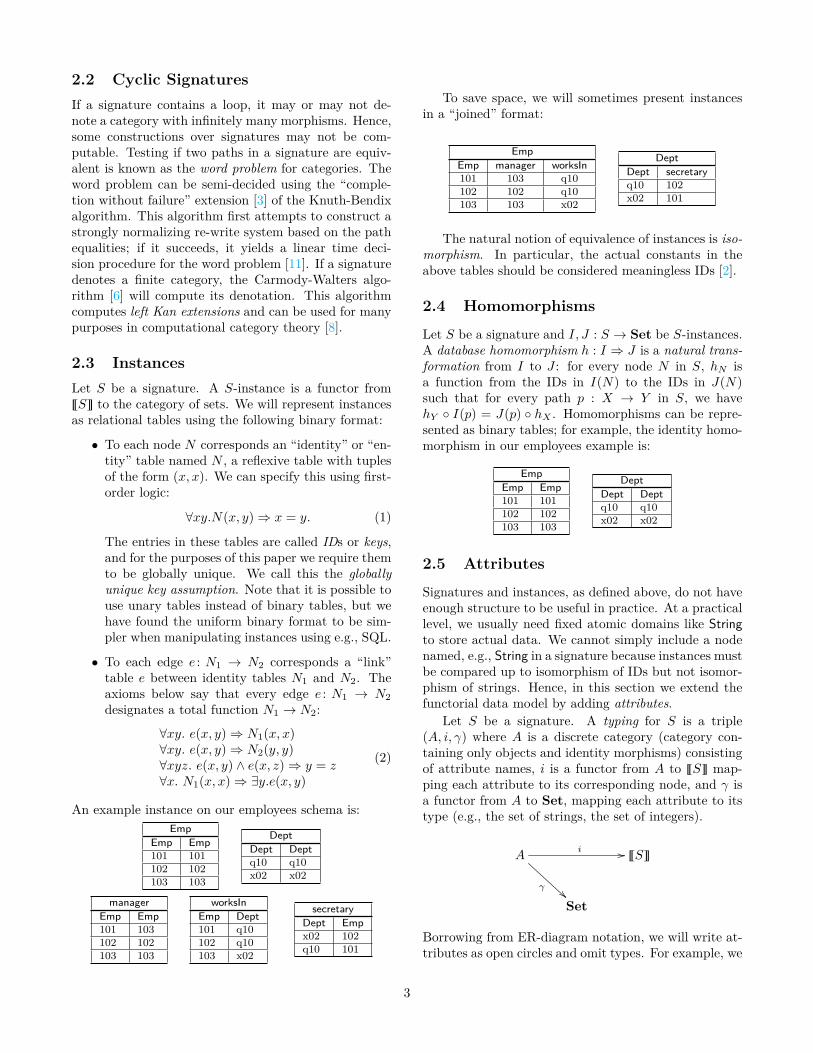
An example instance on our employees schema is:Emp

Emp Emp101 101102 102103 103

DeptDept Deptq10 q10x02 x02

managerEmp Emp101 103102 102103 103

worksInEmp Dept101 q10102 q10103 x02

secretaryDept Empx02 102q10 101

To save space, we will sometimes present instancesin a “joined” format:

EmpEmp manager worksIn101 103 q10102 102 q10103 103 x02

DeptDept secretaryq10 102x02 101

The natural notion of equivalence of instances is iso-morphism. In particular, the actual constants in theabove tables should be considered meaningless IDs [2].

2.4 Homomorphisms

Let S be a signature and I, J : S → Set be S-instances.A database homomorphism h : I ⇒ J is a natural trans-formation from I to J : for every node N in S, hN isa function from the IDs in I(N) to the IDs in J(N)such that for every path p : X → Y in S, we havehY ◦ I(p) = J(p) ◦ hX . Homomorphisms can be repre-sented as binary tables; for example, the identity homo-morphism in our employees example is:

EmpEmp Emp101 101102 102103 103

DeptDept Deptq10 q10x02 x02

2.5 Attributes

Signatures and instances, as defined above, do not haveenough structure to be useful in practice. At a practicallevel, we usually need fixed atomic domains like Stringto store actual data. We cannot simply include a nodenamed, e.g., String in a signature because instances mustbe compared up to isomorphism of IDs but not isomor-phism of strings. Hence, in this section we extend thefunctorial data model by adding attributes.

Let S be a signature. A typing for S is a triple(A, i, γ) where A is a discrete category (category con-taining only objects and identity morphisms) consistingof attribute names, i is a functor from A to ~S� map-ping each attribute to its corresponding node, and γ isa functor from A to Set, mapping each attribute to itstype (e.g., the set of strings, the set of integers).

Ai //

γ!!

~S�

Set

Borrowing from ER-diagram notation, we will write at-tributes as open circles and omit types. For example, we

3

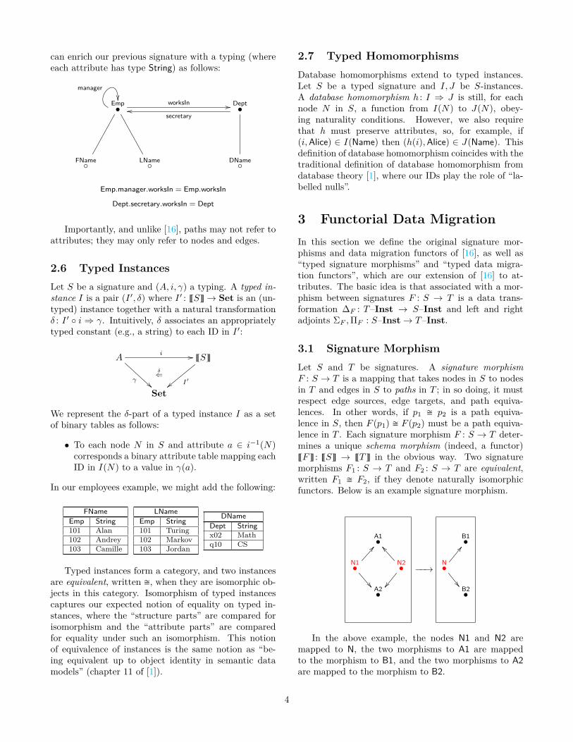
can enrich our previous signature with a typing (whereeach attribute has type String) as follows:

Emp•

worksIn //

manager��

Dept•

secretaryoo

FName◦ LName◦ DName◦

Emp.manager.worksIn = Emp.worksIn

Dept.secretary.worksIn = Dept

Importantly, and unlike [16], paths may not refer toattributes; they may only refer to nodes and edges.

2.6 Typed InstancesLet S be a signature and (A, i, γ) a typing. A typed in-stance I is a pair (I ′, δ) where I ′ : ~S�→ Set is an (un-typed) instance together with a natural transformationδ : I ′ ◦ i ⇒ γ. Intuitively, δ associates an appropriatelytyped constant (e.g., a string) to each ID in I ′:

Ai //

γ!!

δ⇐

~S�

I′||Set

We represent the δ-part of a typed instance I as a setof binary tables as follows:

• To each node N in S and attribute a ∈ i−1(N)corresponds a binary attribute table mapping eachID in I(N) to a value in γ(a).

In our employees example, we might add the following:

FNameEmp String101 Alan102 Andrey103 Camille

LNameEmp String101 Turing102 Markov103 Jordan

DNameDept Stringx02 Mathq10 CS

Typed instances form a category, and two instancesare equivalent, written �, when they are isomorphic ob-jects in this category. Isomorphism of typed instancescaptures our expected notion of equality on typed in-stances, where the “structure parts” are compared forisomorphism and the “attribute parts” are comparedfor equality under such an isomorphism. This notionof equivalence of instances is the same notion as “be-ing equivalent up to object identity in semantic datamodels” (chapter 11 of [1]).

2.7 Typed HomomorphismsDatabase homomorphisms extend to typed instances.Let S be a typed signature and I, J be S-instances.A database homomorphism h : I ⇒ J is still, for eachnode N in S, a function from I(N) to J(N), obey-ing naturality conditions. However, we also requirethat h must preserve attributes, so, for example, if(i,Alice) ∈ I(Name) then (h(i),Alice) ∈ J(Name). Thisdefinition of database homomorphism coincides with thetraditional definition of database homomorphism fromdatabase theory [1], where our IDs play the role of “la-belled nulls”.

3 Functorial Data MigrationIn this section we define the original signature mor-phisms and data migration functors of [16], as well as“typed signature morphisms” and “typed data migra-tion functors”, which are our extension of [16] to at-tributes. The basic idea is that associated with a mor-phism between signatures F : S → T is a data trans-formation ∆F : T–Inst → S–Inst and left and rightadjoints ΣF ,ΠF : S–Inst→ T–Inst.

3.1 Signature MorphismLet S and T be signatures. A signature morphismF : S → T is a mapping that takes nodes in S to nodesin T and edges in S to paths in T ; in so doing, it mustrespect edge sources, edge targets, and path equiva-lences. In other words, if p1 � p2 is a path equiva-lence in S, then F (p1) � F (p2) must be a path equiva-lence in T . Each signature morphism F : S → T deter-mines a unique schema morphism (indeed, a functor)~F� : ~S� → ~T� in the obvious way. Two signaturemorphisms F1 : S → T and F2 : S → T are equivalent,written F1 � F2, if they denote naturally isomorphicfunctors. Below is an example signature morphism.

A1•

N1•

AA

��

N2•

]]

��A2•

−−→

B1•

N•

BB

��B2•

In the above example, the nodes N1 and N2 aremapped to N, the two morphisms to A1 are mappedto the morphism to B1, and the two morphisms to A2are mapped to the morphism to B2.

4

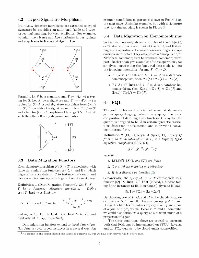
3.2 Typed Signature MorphismsIntuitively, signature morphisms are extended to typedsignatures by providing an additional (node and type-respecting) mapping between attributes. For example,we might have Name and Age attributes in our typingsand map Name to Name and Age to Age:

Name◦

A1•

N1•

>>

N2•

``

~~A2•

Age◦

−−→

Name◦

B1•

N•

??

�� B2•

Age◦

Formally, let S be a signature and Γ := (A, i, γ) a typ-ing for S. Let S′ be a signature and Γ′ := (A′, i′, γ′) atyping for S′. A typed signature morphism from (S,Γ)to (S′,Γ′) consists of a signature morphism F : S → S′

and a functor (i.e. a “morphism of typings”) G : A→ A′

such that the following diagram commutes:

Ai //

γ!!

G

��

~S�

~F �

��

Set

A′

γ′==

i′// ~S′�

3.3 Data Migration FunctorsEach signature morphism F : S → T is associated withthree data migration functors, ∆F ,ΣF , and ΠF , whichmigrate instance data on S to instance data on T andvice versa. A summary is in Figure 1 on the next page.

Definition 1 (Data Migration Functors). Let F : S →T be a (untyped) signature morphism. Define∆F : T–Inst→ S–Inst as:

∆F (I) := I ◦ F : S → SetS

F //

∆F (I)

66TI // Set

and define ΣF ,ΠF : S–Inst → T–Inst to be left andright adjoint to ∆F , respectively.

Data migration functors extend to typed data migra-tion functors over typed instances in a natural way. An

example typed data migration is shown in Figure 2 onthe next page. A similar example, but with a signaturethat contains an edge, is shown in Figure 3.

3.4 Data Migration on HomomorphismsSo far, we have only shown examples of the “object”,or “instance to instance”, part of the ∆, Σ, and Π datamigration operations. Because these data migration op-erations are functors, they also posses a “morphism”, or“database homomorphism to database homomorphism”part. Rather than give examples of these operations, wesimply summarize that the functorial data model admitsthe following operations, for any F : C → D.• If I, J ∈ D–Inst and h : I ⇒ J is a database

homomorphism, then ∆F (h) : ∆F (I)⇒ ∆F (J).

• If I, J ∈ C–Inst and h : I ⇒ J is a database ho-momorphism, then ΣF (h) : ΣF (I) ⇒ ΣF (J) andΠF (h) : ΠF (I)⇒ ΠF (J).

4 FQLThe goal of this section is to define and study an al-gebraic query language where every query denotes acomposition of data migration functors. Our syntax forqueries is designed to build-in certain syntactic restric-tions discussion in this section, and to provide a conve-nient normal form.Definition 2 (FQL Query). A (typed) FQL query Qfrom S to T , denoted Q : S { T , is a triple of typedsignature morphisms (F,G,H):

SF←− S′ G−→ S′′

H−→ T

such that1. ~S�, ~S′�, ~S′′�, and ~T� are finite

2. G’s attribute mapping is a bijection2.

3. H is a discrete op-fibration [4]Semantically, the query Q : S { T corresponds to afunctor ~Q� : S–Inst→ T–Inst (indeed, a functor tak-ing finite instances to finite instances) given as follows:

~Q� := ~ΣH ◦ΠG ◦∆F �

By choosing two of F , G, and H to be the identity, wecan recover ∆, Σ, and Π. However, grouping ∆,Σ, andΠ together like this formalizes a query as a disjoint unionof a join of a projection. Because ∆ and Π commute,we could also formalize a query as a disjoint union of aprojection of a join.

The three conditions above are crucial to ensuringboth that FQL can be implemented on SPCU+keygen,and for FQL queries to be closed under composition:

2All results in this paper should also apply to surjections, but we have only proved the bijective case.

5

Figure 1: Data migration functors induced by a signature morphism F : S → T

Name Symbol Type Idea of definition Relational partnerPullback ∆F ∆F : T–Inst→ S–Inst Composition with F Project

Right Pushforward ΠF ΠF : S–Inst→ T–Inst Right adjoint to ∆F JoinLeft Pushforward ΣF ΣF : S–Inst→ T–Inst Left adjoint to ∆F Union

Figure 2: Data migration example

Name•

Salary•

N1•

GG

>>

N2•

~~Age•

F−−−−→

Name•

Salary•

N•

GG

??

��Age•

N1ID Name Salary1 Alice $1002 Bob $2503 Sue $300

N2ID Age4 205 206 30

↓ ΣF

NID Name Salary Agea Alice $100 null1b Bob $250 null2c Sue $300 null3d null4 null5 20e null6 null7 20f null8 null9 30

∆F←−−

↘ ΠF

NID Name Salary Agea Alice $100 20b Bob $250 20c Sue $300 30

NID Name Salary Agea Alice $100 20b Alice $100 20c Alice $100 30d Bob $250 20e Bob $250 20f Bob $250 30g Sue $300 20h Sue $300 20i Sue $300 30

Figure 3: Data migration example with foreign keys

Name•

Salary•

N1• f //

GG

>>

N2•

~~Age•

F−−−−→

Name•

Salary•

N•

GG

��Age•

N1ID Name Salary f1 Alice $100 42 Bob $250 53 Sue $300 6

N2ID Age4 205 206 30

∆F←−−

ΣF−−→

ΠF−−→

NID Name Salary Agea Alice $100 20b Bob $250 20c Sue $300 30

6

1. Condition 1 ensures that path equivalence in eachsignature is in fact decidable. Moreover, the fiberproduct of two (infinite) finitely-presented cate-gories may not be finitely presented, so it may notbe possible to compute composition queries whenschemas are infinite. Finiteness of schemas alsoensures that Π operations always give finite an-swers. When the target schema is infinite, Π maycreate uncountably infinite result instances. Con-sider the unique signature morphism:

S := s• F−−−→s•

f�� =: T

Here ~T� has morphisms {fn | n ∈ N} so it is infi-nite. Given the two-element instance I : S → Setwith I(s) = {Alice,Bob}, the rowset in ΠF (I)(s)is the (uncountable) set of infinite streams in{Alice,Bob}, i.e. ΠF (I)(s) � I(s)N.

2. Condition 2 ensures that the FQL query is “do-main independent” [1]; i.e., that constants result-ing from any Π operation are contained in the in-put instance. Consider the unique morphism:

S := s• F−−−→ s• − ◦ a (Int) =: T

Given the one-element instance I : S → Set withI(s) = {Alice}, the rowset in ΠF (I)(a) will con-tain, for every integer i, a row (Alicei, i), i.e.,ΠF (I)(a) � {(Alice1, 1), (Alice2, 2), . . .}.

3. Condition 3 ensures “union-compatibility” [1],which allows us to implement Σ using SPCU’sunion operation. A functor F : C → D is called adiscrete op-fibration if, for every object c ∈ C andevery morphism g : d → d′ in D with F (c) = d,there exists a c′ and unique morphism g : c → c′

in C such that F (g) = g. For example, the follow-ing functor, which maps as to A, bs to B, etc. isa discrete op-fibration:

C :=

b1•a1•

h1 //g1oo c1•

b2•a2•

g2oo h2 // c2•

a3•g3

hh

h3

((

c3•

c4•

F

��

D := B•

A• H //Goo C

•

Intuitively, F : C → D is a discrete op-fibrationif “the columns in each table T of D are exactlymatched by the columns in each table in C map-ping to T .” Since a1, a2, a3 7→ A, they must havethe same column structure and they do: each hastwo non-ID columns. Similarly each of the bi andeach of the ci have no non-ID columns, just liketheir images in D.

Remark. ΣF is defined for any F , not just fordiscrete op-fibrations. However, such unrestrictedΣs cannot be implemented using SPCU+keygen(even if we allow OUTER UNION), and FQL queriesthat use such Σs are not closed under composition.

4.1 Composition

Theorem 1 (Closure under composition). Given any(typed) FQL queries f : S { X and g : X { T , we cancompute an FQL query g · f : S { T such that

~g · f� � ~g� ◦ ~f�

Sketch of proof. Following the proof in [9, Proposition1.1.2], it suffices to show the Beck-Chevalley conditionshold for ∆ and its adjoints, and that dependent sumsdistribute over dependent products when the former areindexed by discrete op-fibrations. The proof and algo-rithm are given in the appendix as Theorem 9.2.6. �

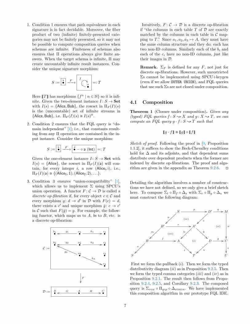
Detailing the algorithm involves a number of construc-tions we have not defined, so we only give a brief sketchhere. To compose Σt ◦ Πf ◦ ∆s with Σv ◦ Πg ◦ ∆u wemust construct the following diagram:

Np //

n

~~(iv)

D′q //

e~~

(ii)

M

w

��

B′r //

m

~~(iii)

A′

k

h

~~(i)B

s

��

f // A

t

D

u}}

g // C

v

��S T U

First we form the pullback (i). Then we form the typeddistributivity diagram (ii) as in Proposition 9.2.5. Thenwe form the typed comma categories (iii) and (iv) as inProposition 9.2.1. The result then follows from Propo-sition 9.2.4, 9.2.5, and Corollary 9.2.3. The composedquery is Σv◦w ◦ Πq◦p ◦ ∆s◦m◦n. We have implementedthis composition algorithm in our prototype FQL IDE.

7

5 FQL in SPCU+keygenIn this section we let F : S → T be a typed signaturemorphism and we define SPCU+keygen translations for∆F , ΣF , and ΠF . By an SPCU+keygen program wemean a list of SQL expressions, where each SQL ex-pression is one of the following:

1. A conjuctive query over base tables; i.e., a SQLexpression of the form SELECT DISTINCT - FROM- WHERE -.

2. A union of SPCU-keygen expressions; i.e., a SQLexpression - UNION - .

3. A globally-unique ID generation operation (key-gen) that appends to a given table a new columnwith globally unique IDs. To implement keygen inSQL, we first initialize a global variable, using, forexample, the following MySQL code: SET @guid:= 0. Then, to implement keygen we incrementthis global variable. For example, to add a col-umn “c” of new unique IDs to a table “t” withone column called “col”, we would generate:

SELECT col, @guid:=@guid+1 AS c FROM t

4. A CREATE TABLE followed by an INSERT INTO ofan SPCU-keygen expression.

A SQL/SPCU+keygen program that implements afunctorial data migration S–Inst → T–Inst operatesover a SQL schema containing one binary table for eachnode, edge, and attribute in S, and stores one binarytable for each node, edge, and attribute in T .

5.1 Translating ∆Theorem 2. We can compute a SPCU+keygen pro-gram [F ]∆ such that for every T -instance I ∈ T–Inst,we have ∆F (I) � [F ]∆(I).

Proof. See Construction 8.2.1. �

We sketch the algorithm as follows. We are given aT -instance I, presented as a set of functional binary ta-bles, and are tasked with creating the S-instance ∆F (I).We describe the result of ∆F (I) on each table in the re-sult instance by examining the schema S:

• for each node N in S, the binary table ∆F (N) isthe binary table I(F (N)).

• for each attribute A in S, the binary table ∆F (A)is the binary table I(F (A)).

• Each edge e : X → Y in S maps to a pathF (e) : F (X) → F (Y ) in T . We compose the bi-nary edges tables making up the path F (e), andthat becomes the binary table ∆F (e).

The SQL generation algorithm for ∆ above (and Σ, be-low) does not maintain the globally unique ID require-ment. For example, ∆ can copy tables. Hence we mustalso generate SQL to restore the unique ID invariant.

5.2 Translating ΣTheorem 3. Suppose F is a discrete op-fibration. Thenwe can compute a SPCU+keygen program [F ]Σ suchthat for every S-instance I ∈ S–Inst, ΣF (I) � [F ]Σ(I).

Proof. See Construction 8.2.10. �

We sketch the algorithm as follows. We are given aS-instance I, presented as a set of functional binary ta-bles, and are tasked with creating the T -instance ΣF (I).We describe the result of ΣF (I) on each table in the re-sult instance by examining the schema T :

• for each node N in T , the binary table ΣF (N) isthe union of the binary node tables in I that mapto N via F .

• for each attribute A in T , the binary table ΣF (A)is the union of the binary attribute tables in I thatmap to A via F .

• Let e : X → Y be an edge in T . We know that foreach c ∈ F−1(X) there is at least one path pc inS such that F (pc) � e. Compose pc to a single bi-nary table, and define ΣF (e) to be the union overall such c. The choice of pc will not matter.

5.3 Translating ΠTheorem 4. Suppose ~S� and ~T� are finite, and Fhas a bijective attribute mapping. Then we can com-pute a SPCU+keygen program [F ]Π such that for everyS-instance I ∈ S–Inst, we have ΠF (I) � [F ]Π(I).

Proof. See Construction 8.2.14. �

The algorithm for ΠF is more complex than for ∆F

and ΣF . It makes use of comma categories, which wehave not defined, as well as “limit tables”, which are asort of “join all”. We define these now.

Let B be a typed signature and H a typed B-instance. The limit table limB is computed as follows.First, take the cartesian product of every node table inB, and naturally join the attribute tables of B. Then,for each edge e : n1 → n2 filter the table by n1 = n2.This filtered table is the limit table limB .

Let S : A → C and T : B → C be functors.The comma category (S ↓ T ) has for objects triples(α, β, f), with α an object in A, β an object in B, andf : S(α) → T (β) a morphism in C. The morphismsfrom (α, β, f) to (α′, β′, f ′) are all the pairs (g, h) whereg : α → α′ and h : β → β′ are morphisms in A and Brespectively such that T (h) ◦ f = f ′ ◦ S(g).

8

The algorithm for ΠF proceeds as follows. First, forevery object d ∈ T we consider the comma categoryBd := (d ↓ F ) and its projection functor qd : (d ↓ F )→C. (Here we treat d as a functor from the empty cat-egory). Let Hd := I ◦ qd : Bd → Set, constructed bygenerating SQL for ∆qd(I). We say that the limit ta-ble for d is limBdHd, as described above. Now we candescribe the target tables in T :

• for each node N in T , generate globally uniqueIDs for each row in the limit table for N . TheseIDs are ΠF (N).

• for each attribute A off N in T , ΠF (A) will be aprojection from the limit table for N .

• for each edge e : X → Y in T , ΠF (e) will be a mapfrom X to Y given by joining the limit tables forX and Y on columns which “factor through” e.

Remark. Our SPCU+keygen generation algo-rithms for ∆ and Σ work even when ~S� and ~T� areinfinite, but this is not the case for Π. But if we are will-ing to take on infinite SQL queries, we have Π in gen-eral; see Construction 8.2.14. An interesting directionfor future work is to relate these infinite SQL queries torecursive languages such as Datalog.

5.4 Translating Functorial Data Migra-tions of Homomorphisms

We can also generate SPCU+keygen to implement datamigrations of homomorphisms (c.f. section 3.4).

Theorem 5. For all T -instances I, J ∈ T–Instand homomorphisms h : I ⇒ J , we can computea SPCU+keygen program [F ]∆ such that ∆F (h) �[F ]∆(h), and similarly for ΣF ,ΠF .

Proof. See Constructions 8.2.1, 8.2.10, and 8.2.14. �

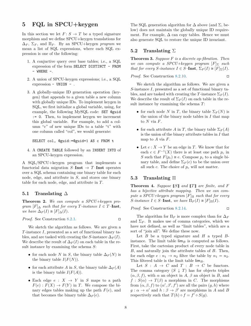
6 SPCU in FQLTo implement SPCU using FQL, we must encode rela-tional schemas as signatures with a single “active do-main” [1] attribute. For example, a schema with tworelations R(c1, . . . , cn) and R′(c′1, . . . , c′n′) becomes:

R•

c1++

···

cn

��

R′•c′n′

��···

c′1ssD•

A◦

We might expect that the c1, . . . , cn would be at-tributes of node R, and hence there would be no nodeD, but that does not work: attributes may not be (di-rectly) joined on. Instead, we must think of each columnof R as a mapping from R’s domain to IDs in D, and Aas a mapping from IDs in D to constants. Note that Aneed not be injective; our constructions below will not ingeneral maintain injectiveness of A (although injective-ness can be recovered using the dedup operation definedin the next section). We will write [R] for the encodingof a relational schema R and [I] for the encoding of arelational R-instance I.

6.1 SPCU in FQL (Bag Semantics)FQL can implement SPCU queries under bag semanticsdirectly using the above encoding. In what follows wewill omit the attribute A from the diagrams. We mayexpress the (bag) operations π, σ,×,+ as follows:

• Let R be a table. We can express πi1,...,ikR as ∆F ,where F is any functor sending πR to R and D toD in the following diagram:

πR•

i1

��··· ik

��D•

F−−−→

R•

c1

��··· cn

��D•

This construction is only appropriate for bag se-mantics because πR will have the same number ofrows as R.

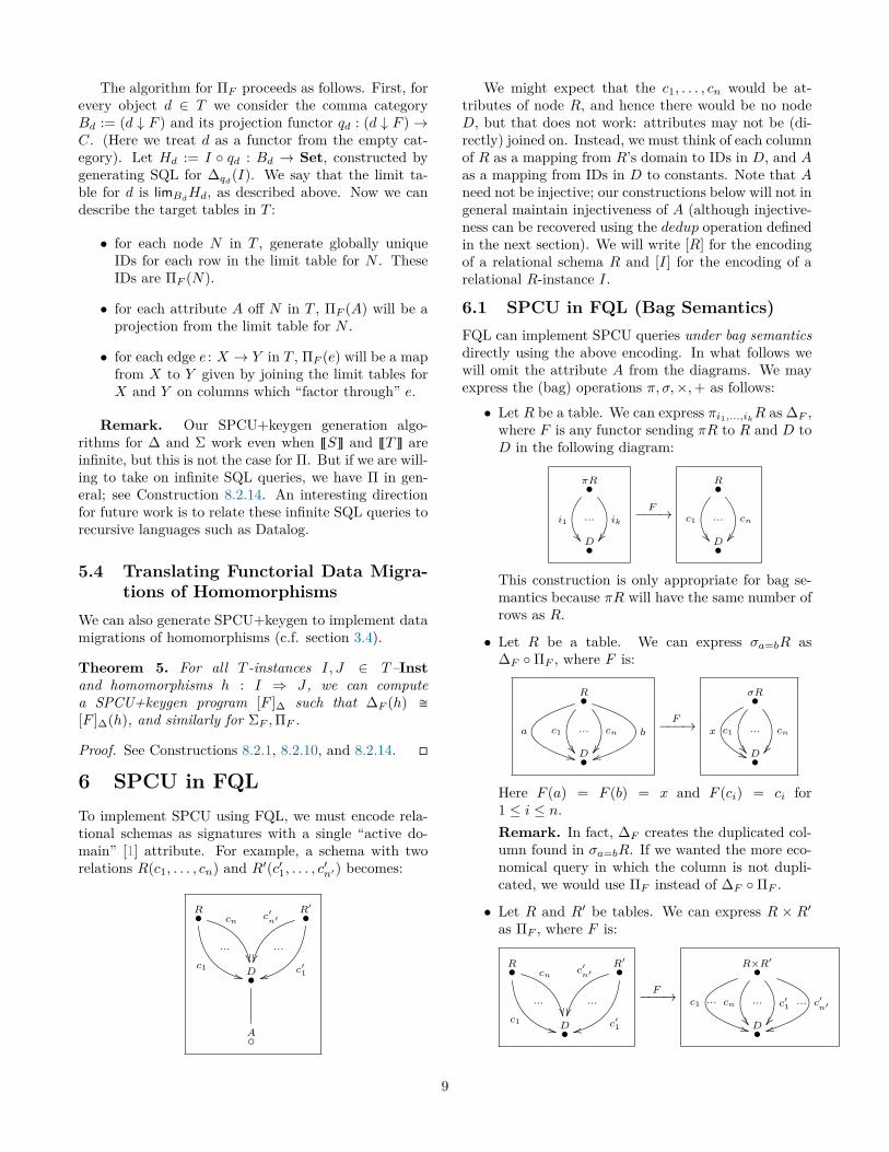
• Let R be a table. We can express σa=bR as∆F ◦ΠF , where F is:

R•

a

**

c1

��··· cn

��b

ttD•

F−−−→

σR•

x

''

c1

��··· cn

��D•

Here F (a) = F (b) = x and F (ci) = ci for1 ≤ i ≤ n.Remark. In fact, ∆F creates the duplicated col-umn found in σa=bR. If we wanted the more eco-nomical query in which the column is not dupli-cated, we would use ΠF instead of ∆F ◦ΠF .

• Let R and R′ be tables. We can express R × R′as ΠF , where F is:

R•

c1++

···

cn

��

R′•c′n′

��···

c′1ssD•

F−−−→

R×R′•

c1

**

··· cn

��··· c′1 ···

��c′n′

ttD•

9

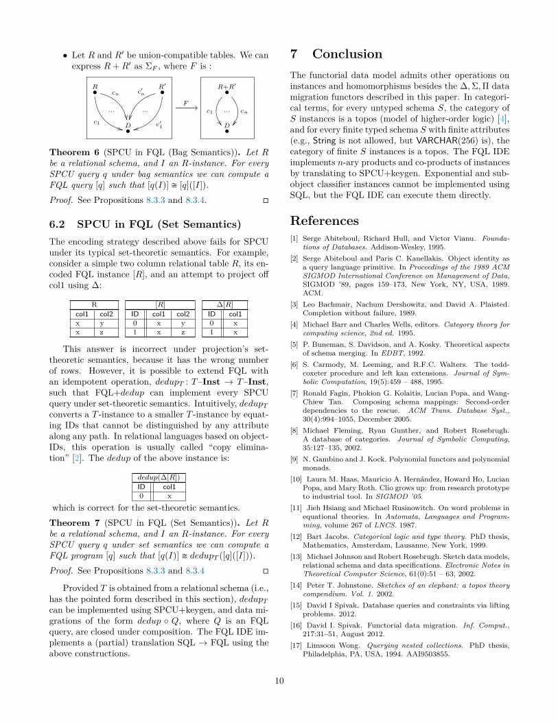
• Let R and R′ be union-compatible tables. We canexpress R+R′ as ΣF , where F is :

R•

c1++

···

cn

��

R′•c′n

��···

c′1ssD•

F−−−→

R+R′•

c1

��··· cn

��D•

Theorem 6 (SPCU in FQL (Bag Semantics)). Let Rbe a relational schema, and I an R-instance. For everySPCU query q under bag semantics we can compute aFQL query [q] such that [q(I)] � [q]([I]).Proof. See Propositions 8.3.3 and 8.3.4. �

6.2 SPCU in FQL (Set Semantics)The encoding strategy described above fails for SPCUunder its typical set-theoretic semantics. For example,consider a simple two column relational table R, its en-coded FQL instance [R], and an attempt to project offcol1 using ∆:

Rcol1 col2x yx z

[R]ID col1 col20 x y1 x z

∆[R]ID col10 x1 x

This answer is incorrect under projection’s set-theoretic semantics, because it has the wrong numberof rows. However, it is possible to extend FQL withan idempotent operation, dedupT : T–Inst → T–Inst,such that FQL+dedup can implement every SPCUquery under set-theoretic semantics. Intuitively, dedupTconverts a T -instance to a smaller T -instance by equat-ing IDs that cannot be distinguished by any attributealong any path. In relational languages based on object-IDs, this operation is usually called “copy elimina-tion” [2]. The dedup of the above instance is:

dedup(∆[R])ID col10 x

which is correct for the set-theoretic semantics.Theorem 7 (SPCU in FQL (Set Semantics)). Let Rbe a relational schema, and I an R-instance. For everySPCU query q under set semantics we can compute aFQL program [q] such that [q(I)] � dedupT ([q]([I])).Proof. See Propositions 8.3.3 and 8.3.4 �

Provided T is obtained from a relational schema (i.e.,has the pointed form described in this section), dedupTcan be implemented using SPCU+keygen, and data mi-grations of the form dedup ◦ Q, where Q is an FQLquery, are closed under composition. The FQL IDE im-plements a (partial) translation SQL → FQL using theabove constructions.

7 ConclusionThe functorial data model admits other operations oninstances and homomorphisms besides the ∆,Σ,Π datamigration functors described in this paper. In categori-cal terms, for every untyped schema S, the category ofS instances is a topos (model of higher-order logic) [4],and for every finite typed schema S with finite attributes(e.g., String is not allowed, but VARCHAR(256) is), thecategory of finite S instances is a topos. The FQL IDEimplements n-ary products and co-products of instancesby translating to SPCU+keygen. Exponential and sub-object classifier instances cannot be implemented usingSQL, but the FQL IDE can execute them directly.

References[1] Serge Abiteboul, Richard Hull, and Victor Vianu. Founda-

tions of Databases. Addison-Wesley, 1995.[2] Serge Abiteboul and Paris C. Kanellakis. Object identity as

a query language primitive. In Proceedings of the 1989 ACMSIGMOD International Conference on Management of Data,SIGMOD ’89, pages 159–173, New York, NY, USA, 1989.ACM.

[3] Leo Bachmair, Nachum Dershowitz, and David A. Plaisted.Completion without failure, 1989.

[4] Michael Barr and Charles Wells, editors. Category theory forcomputing science, 2nd ed. 1995.

[5] P. Buneman, S. Davidson, and A. Kosky. Theoretical aspectsof schema merging. In EDBT, 1992.

[6] S. Carmody, M. Leeming, and R.F.C. Walters. The todd-coxeter procedure and left kan extensions. Journal of Sym-bolic Computation, 19(5):459 – 488, 1995.

[7] Ronald Fagin, Phokion G. Kolaitis, Lucian Popa, and Wang-Chiew Tan. Composing schema mappings: Second-orderdependencies to the rescue. ACM Trans. Database Syst.,30(4):994–1055, December 2005.

[8] Michael Fleming, Ryan Gunther, and Robert Rosebrugh.A database of categories. Journal of Symbolic Computing,35:127–135, 2002.

[9] N. Gambino and J. Kock. Polynomial functors and polynomialmonads.

[10] Laura M. Haas, Mauricio A. Hernandez, Howard Ho, LucianPopa, and Mary Roth. Clio grows up: from research prototypeto industrial tool. In SIGMOD ’05.

[11] Jieh Hsiang and Michael Rusinowitch. On word problems inequational theories. In Automata, Languages and Program-ming, volume 267 of LNCS. 1987.

[12] Bart Jacobs. Categorical logic and type theory. PhD thesis,Mathematics, Amsterdam, Lausanne, New York, 1999.

[13] Michael Johnson and Robert Rosebrugh. Sketch data models,relational schema and data specifications. Electronic Notes inTheoretical Computer Science, 61(0):51 – 63, 2002.

[14] Peter T. Johnstone. Sketches of an elephant: a topos theorycompendium. Vol. 1. 2002.

[15] David I Spivak. Database queries and constraints via liftingproblems. 2012.

[16] David I. Spivak. Functorial data migration. Inf. Comput.,217:31–51, August 2012.

[17] Limsoon Wong. Querying nested collections. PhD thesis,Philadelphia, PA, USA, 1994. AAI9503855.

10

8 Categorical constructions for data migrationHere we give many standard definitions from category theory and a few less-than-standard (or original) results. The proofs often assume more knowledge than the defi-nitions do. Let us also note our use of the term essential, which basically means “up toisomorphism”. Thus an object X having a certain property is essentially unique if everyother object having that property is isomorphic to X; an object X is in the essentialimage of some functor if it is isomorphic to an object in the image of that functor; etc.

8.1 Basic constructionsDefinition 8.1.1 (Fiber products of sets). Suppose given the diagram of sets and func-tions as to the left in (3).

B

g

��

A×C Bf ′ //

h

##g′

��

B

g

��A

f// C A

f// C

(3)

Its fiber product is the commutative diagram to the right in (3), where we define

A×C B := {(a, c, b) | f(a) = c = g(b)}

and f ′, g′, and h = g ◦ f ′ = f ◦ g′ are the obvious projections (e.g. f ′(a, c, b) = b). Wesometimes refer to just (A×C B, f ′, g′, h) or even to A×C B as the fiber product.

Example 8.1.2 (Chain signatures). Let n ∈ N be a natural number. The chain signatureon n arrows, denoted −→n , 3 is the graph

0• // 1• // · · · // n•

with no path equivalences. One can check that −→n has(n+2

2)-many paths.

The chain signature −→0 is the terminal object in the category of signatures.A signature morphism c : −→0 → C can be identified with an object in C. A signature

morphism f : −→1 → C can be identified with a morphism in C. It is determined up topath equivalence by a pair (n, p) where n ∈ N is a natural number and p : −→n → C is amorphism of graphs.

Definition 8.1.3 (Fiber product of signatures). Suppose given the diagram of signaturesand signatures mappings as to the left in (4).

B

g

��

A×C Bf ′ //

h

##g′

��

B

g

��A

f// C A

f// C

(4)

3The chain signature −→n is often denoted [n] in the literature, but we did not want to further overloadthe bracket [-] notation

11

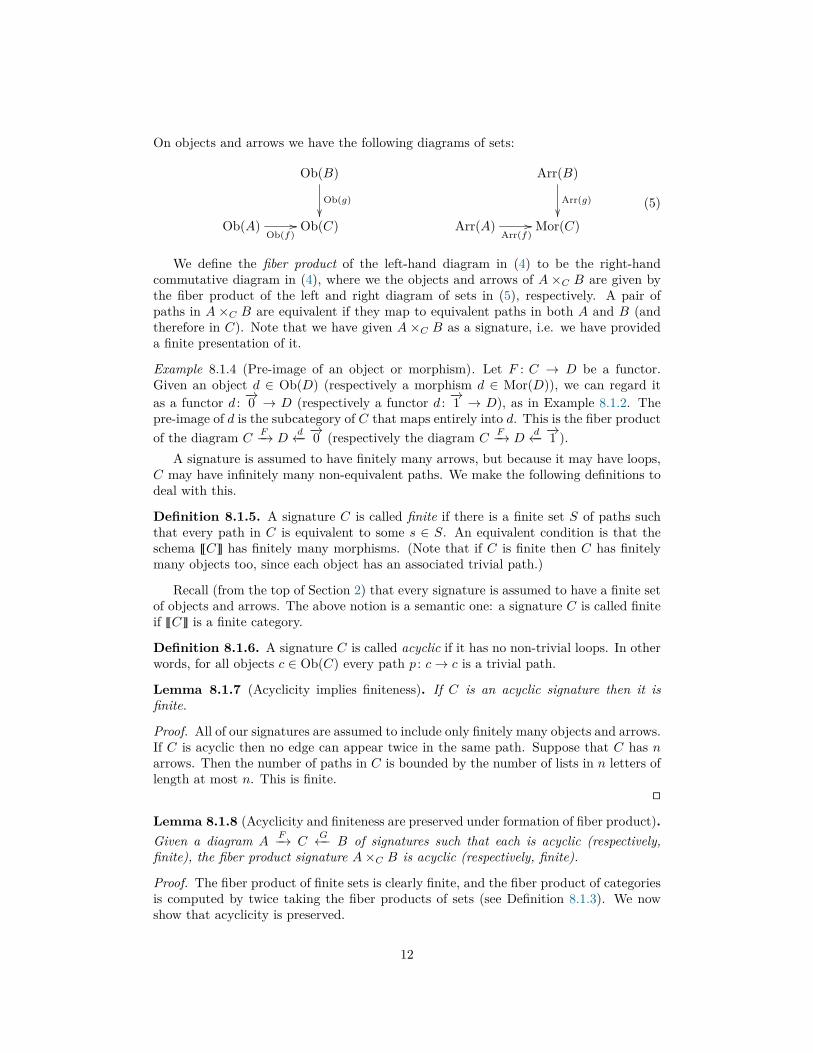
On objects and arrows we have the following diagrams of sets:

Ob(B)

Ob(g)��

Ob(A)Ob(f)

// Ob(C)

Arr(B)

Arr(g)��

Arr(A)Arr(f)

// Mor(C)

(5)

We define the fiber product of the left-hand diagram in (4) to be the right-handcommutative diagram in (4), where we the objects and arrows of A ×C B are given bythe fiber product of the left and right diagram of sets in (5), respectively. A pair ofpaths in A ×C B are equivalent if they map to equivalent paths in both A and B (andtherefore in C). Note that we have given A×C B as a signature, i.e. we have provideda finite presentation of it.

Example 8.1.4 (Pre-image of an object or morphism). Let F : C → D be a functor.Given an object d ∈ Ob(D) (respectively a morphism d ∈ Mor(D)), we can regard itas a functor d : −→0 → D (respectively a functor d : −→1 → D), as in Example 8.1.2. Thepre-image of d is the subcategory of C that maps entirely into d. This is the fiber productof the diagram C

F−→ Dd←− −→0 (respectively the diagram C

F−→ Dd←− −→1 ).

A signature is assumed to have finitely many arrows, but because it may have loops,C may have infinitely many non-equivalent paths. We make the following definitions todeal with this.

Definition 8.1.5. A signature C is called finite if there is a finite set S of paths suchthat every path in C is equivalent to some s ∈ S. An equivalent condition is that theschema ~C� has finitely many morphisms. (Note that if C is finite then C has finitelymany objects too, since each object has an associated trivial path.)

Recall (from the top of Section 2) that every signature is assumed to have a finite setof objects and arrows. The above notion is a semantic one: a signature C is called finiteif ~C� is a finite category.

Definition 8.1.6. A signature C is called acyclic if it has no non-trivial loops. In otherwords, for all objects c ∈ Ob(C) every path p : c→ c is a trivial path.

Lemma 8.1.7 (Acyclicity implies finiteness). If C is an acyclic signature then it isfinite.

Proof. All of our signatures are assumed to include only finitely many objects and arrows.If C is acyclic then no edge can appear twice in the same path. Suppose that C has narrows. Then the number of paths in C is bounded by the number of lists in n letters oflength at most n. This is finite.

�

Lemma 8.1.8 (Acyclicity and finiteness are preserved under formation of fiber product).Given a diagram A

F−→ CG←− B of signatures such that each is acyclic (respectively,

finite), the fiber product signature A×C B is acyclic (respectively, finite).

Proof. The fiber product of finite sets is clearly finite, and the fiber product of categoriesis computed by twice taking the fiber products of sets (see Definition 8.1.3). We nowshow that acyclicity is preserved.

12

Let Loop denote the signature

Loop :=s•

f�� (6)

A category C is acyclic if and only if every functor L : Loop → C factors through theunique functor Loop → −→0 , i.e. if and only if every loop is a trivial path. The resultfollows by the universal property for fiber products.

�

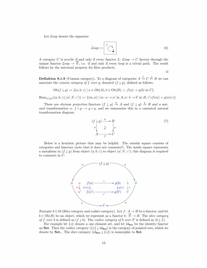
Definition 8.1.9 (Comma category). To a diagram of categories A f−→ Cg←− B we can

associate the comma category of f over g, denoted (f ↓ g), defined as follows.

Ob(f ↓ g) := {(a, b, γ) | a ∈ Ob(A), b ∈ Ob(B), γ : f(a)→ g(b) in C}

Hom(f↓g)((a, b, γ), (a′, b′, γ′)) := {(m,n) | m : a→ a′ in A,n : b→ b′ in B, γ′◦f(m) = g(n)◦γ}

There are obvious projection functors (f ↓ g) p−→ A and (f ↓ g) q−→ B and a nat-ural transformation α : f ◦ p → g ◦ q, and we summarize this in a canonical naturaltransformation diagram

(f ↓ g) q //

p

��

α

t

B

g

��A

f// C

(7)

Below is a heuristic picture that may be helpful. The outside square consists ofcategories and functors (note that it does not commute!). The inside square representsa morphism in (f ↓ g) from object (a, b, γ) to object (a′, b′, γ′); this diagram is requiredto commute in C.

(f ↓ g)p

q

��A

f00

am ��

f(a) γ //

f(m) ��

g(b)g(n)��

bn��

B

goo

a′ f(a′)γ′

// g(b′) b′

C

Example 8.1.10 (Slice category and coslice category). Let f : A→ B be a functor, and letb ∈ Ob(B) be an object, which we represent as a functor b : −→0 → B. The slice categoryof f over b is defined as (f ↓ b). The coslice category of b over F is defined as (b ↓ f).

For example let {∗} denote a one element set, and let idSet be the identity functoron Set. Then the coslice category ({∗} ↓ idSet) is the category of pointed sets, which wedenote by Set∗. The slice category (idSet ↓ {∗}) is isomorphic to Set.

13

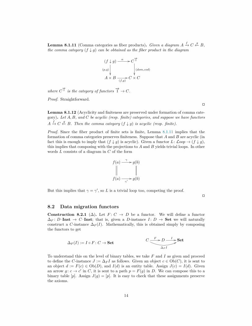
Lemma 8.1.11 (Comma categories as fiber products). Given a diagram Af−→ C

g←− B,the comma category (f ↓ g) can be obtained as the fiber product in the diagram

(f ↓ g) α //

(p,q)��

C−→1

(dom,cod)��

A×B(f,g)

// C × C

where C−→1 is the category of functors −→1 → C.

Proof. Straightforward.�

Lemma 8.1.12 (Acyclicity and finiteness are preserved under formation of comma cate-gory). Let A,B, and C be acyclic (resp. finite) categories, and suppose we have functorsA

f−→ Cg←− B. Then the comma category (f ↓ g) is acyclic (resp. finite).

Proof. Since the fiber product of finite sets is finite, Lemma 8.1.11 implies that theformation of comma categories preserves finiteness. Suppose that A and B are acyclic (infact this is enough to imply that (f ↓ g) is acyclic). Given a functor L : Loop→ (f ↓ g),this implies that composing with the projections to A and B yields trivial loops. In otherwords L consists of a diagram in C of the form

f(a) γ // g(b)

f(a)γ′// g(b)

But this implies that γ = γ′, so L is a trivial loop too, competing the proof.�

8.2 Data migration functorsConstruction 8.2.1 (∆). Let F : C → D be a functor. We will define a functor∆F : D–Inst → C–Inst; that is, given a D-instance I : D → Set we will naturallyconstruct a C-instance ∆F (I). Mathematically, this is obtained simply by composingthe functors to get

∆F (I) := I ◦ F : C → Set CF //

∆F I

66DI // Set

To understand this on the level of binary tables, we take F and I as given and proceedto define the C-instance J := ∆F I as follows. Given an object c ∈ Ob(C), it is sent toan object d := F (c) ∈ Ob(D), and I(d) is an entity table. Assign J(c) = I(d). Givenan arrow g : c → c′ in C, it is sent to a path p = F (g) in D. We can compose this to abinary table [p]. Assign J(g) = [p]. It is easy to check that these assignments preservethe axioms.

14

Lemma 8.2.2 (Finiteness is preserved under ∆). Suppose that C and D are finitecategories and F : C → D is a functor. If I : D → Set is a finite D-instance then ∆F Iis a finite C-instance.

Proof. This follows by construction: every object and arrow in C is assigned some finitejoin of the tables associated to objects and arrows in D, and finite joins of finite tablesare finite.

�

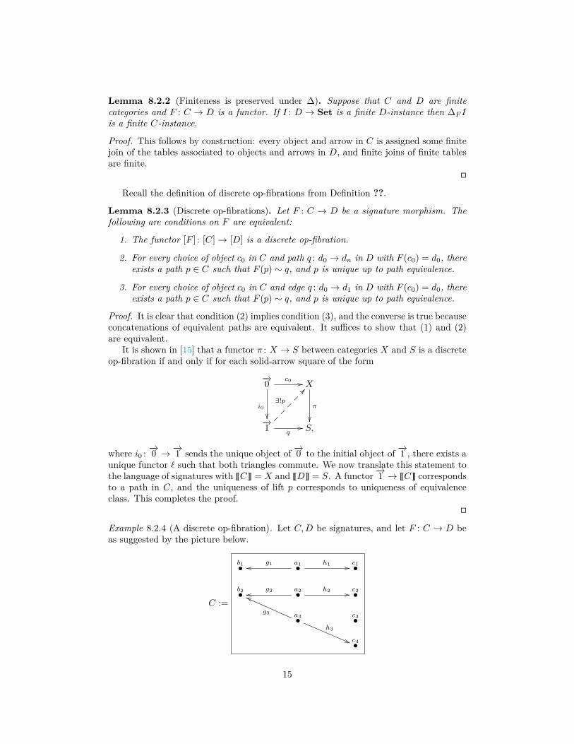
Recall the definition of discrete op-fibrations from Definition ??.

Lemma 8.2.3 (Discrete op-fibrations). Let F : C → D be a signature morphism. Thefollowing are conditions on F are equivalent:

1. The functor [F ] : [C]→ [D] is a discrete op-fibration.

2. For every choice of object c0 in C and path q : d0 → dn in D with F (c0) = d0, thereexists a path p ∈ C such that F (p) ∼ q, and p is unique up to path equivalence.

3. For every choice of object c0 in C and edge q : d0 → d1 in D with F (c0) = d0, thereexists a path p ∈ C such that F (p) ∼ q, and p is unique up to path equivalence.

Proof. It is clear that condition (2) implies condition (3), and the converse is true becauseconcatenations of equivalent paths are equivalent. It suffices to show that (1) and (2)are equivalent.

It is shown in [15] that a functor π : X → S between categories X and S is a discreteop-fibration if and only if for each solid-arrow square of the form

−→0 c0 //

i0

��

X

π

��−→1

∃!p

??

q// S,

where i0 : −→0 → −→1 sends the unique object of −→0 to the initial object of −→1 , there exists aunique functor ` such that both triangles commute. We now translate this statement tothe language of signatures with ~C� = X and ~D� = S. A functor −→1 → ~C� correspondsto a path in C, and the uniqueness of lift p corresponds to uniqueness of equivalenceclass. This completes the proof.

�

Example 8.2.4 (A discrete op-fibration). Let C,D be signatures, and let F : C → D beas suggested by the picture below.

C :=

b1• a1• h1 //g1oo c1•

b2• a2•g2oo h2 // c2•

a3•g3

hh

h3

((

c3•

c4•

15

F

��

D := B• A• H //Goo C•

This is a discrete op-fibration.Corollary 8.2.5 (Pre-image of an object under a discrete op-fibration is discrete). LetF : C → D be a discrete op-fibration and let d ∈ Ob(D) be an object. Then the pre-imageF−1(d) is a discrete signature (i.e. every path in F−1(d) is equivalent to a trivial path).Proof. For any object d ∈ Ob(D) the pre-image F−1(d) is either empty or not. If it isempty, then it is discrete. If F−1(d) is non-empty, let e : c0 → c1 be an edge in it. ThenF (e) = d = F (c0) so we have an equivalence e ∼ c0 by Lemma 8.2.3.

�

Example 8.2.6. Let F : A → B be a functor. For any object b ∈ B, considered as afunctor b : −→0 → B, the induced functor (b ↓ F ) → B is a discrete op-fibration. Indeed,given an object b g−→ F (a) in (b ↓ F ) and a morphism h : a → a′ in A, there is a uniquemap b

g−→ F (a) F (h)−−−→ F (a′) over it.Definition 8.2.7. A signature C is said to have non-redundant edges if it satisfies thefollowing condition for every edge e and path p in C: If e ∼ p, then p has length 1 ande = p.Proposition 8.2.8. Every acyclic signature is equivalent to a signature with non-redundantedges.Proof. The important observation is that if C is acyclic then for any edge e and path p inC, if e is an edge in p and e ∼ p then e = p. Thus, we know that if C is acyclic and e ∼ pthen e is not in p. So enumerate the edges of C as EC := {e1, . . . , en}. If e1 is equivalentto a path in EC − {e1} then there is an equivalence of signatures C �−→ C − {e1} =: C1;if not, let C1 := C. Proceed by induction to remove each ei that is equivalent to a pathin Ci−1, and at the end no edge will be redundant.

�

Corollary 8.2.9 (Discrete op-fibrations and preservation of path length). If C and Dhave non-redundant edges and F : C → D is a discrete op-fibration, then for every choiceof object c0 in C and path q = d0.e

′1.e′2. . . . .e

′n of length n in D with F (c0) = d0, there

exists a unique path p = c0.e1.e2. . . . .en of length n in C such that F (ei) = e′i for each1 ≤ i ≤ n, so in particular F (p) = q.Proof. Let c0, d0, and q be as in the hypothesis. We proceed by induction on n, thelength of q. In the base case n = 0 then Corollary 8.2.5 implies that every edge inF−1(d0) is equivalent to the trivial path c0, so the result follows by the non-redundancyof edges in C. Suppose the result holds for some n ∈ N. To prove the result for n+ 1 itsuffices to consider the final edge of q, i.e. we assume that q = e′ is simply an edge. ByLemma 8.2.3 there exists a path p ∈ C such that F (p) ∼ e′, so by non-redundancy inD we know that F (p) has length 1. This implies that for precisely one edge ei in p wehave F (ei) = e′, and for all other edges ej in p we have F (ej) is a trivial path. But bythe base case this implies that p has length 1, completing the proof.

�

16

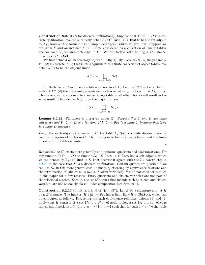
Construction 8.2.10 (Σ for discrete opfibrations). Suppose that F : C → D is a dis-crete op-fibration. We can succinctly define ΣF : C–Inst→ D–Inst to be the left adjointto ∆F , however the formula has a simple description which we give now. Suppose weare given F and an instance I : C → Set, considered as a collection of binary tables,one for each object and each edge in C. We are tasked with finding a D-instance,J := ΣF I : D → Set.

We first define J on an arbitrary object d ∈ Ob(D). By Corollary 8.2.5, the pre-imageF−1(d) is discrete in C; that is, it is equivalent to a finite collection of object tables. Wedefine J(d) to be the disjoint union

J(d) :=∐

c∈F−1(d)

I(c).

Similarly, let e : d→ d′ be an arbitrary arrow in D. By Lemma 8.2.3 we know that foreach c ∈ F−1(d) there is a unique equivalence class of paths pc in C such that F (pc) ∼ e.Choose one, and compose it to a single binary table — all other choices will result in thesame result. Then define J(e) to be the disjoint union

J(e) :=∐

c∈F−1(d)

I(pc).

Lemma 8.2.11 (Finiteness is preserved under Σ). Suppose that C and D are finitecategories and F : C → D is a functor. If I : C → Set is a finite C-instance then ΣF Iis a finite D instance.

Proof. For each object or arrow d in D, the table ΣF I(d) is a finite disjoint union ofcomposition-joins of tables in C. The finite join of finite tables is finite, and the finiteunion of finite tables is finite.

�

Remark 8.2.12 (Σ exists more generally and performs quotients and skolemization). Forany functor F : C → D the functor ∆F : D–Inst → C–Inst has a left adjoint, whichwe can denote by ΣF : C–Inst→ D–Inst because it agrees with the ΣF constructed in8.2.10 in the case that F is a discrete op-fibration. Certain queries are possible if wecan use ΣF in this more general case—namely, quotienting by equivalence relations andthe introduction of labeled nulls (a.k.a. Skolem variables). We do not consider it muchin this paper for a few reasons. First, quotients and skolem variables are not part ofthe relational algebra. Second, the set of queries that include such quotients and skolemvariables are not obviously closed under composition (see Section 7).

Construction 8.2.13 (Limit as a kind of “join all”). Let B be a signature and let Hbe a B-instance. The functor [H] : [B]→ Set has a limit limB H ∈ Ob(Set), which canbe computed as follows. Forgetting the path equivalence relations, axioms (1) and (2)imply that H consists of a set {N1, . . . , Nm} of node tables, a set {e1, . . . , en} of edgetables, and functions s, t : {1, . . . , n} → {1, . . . ,m} such that for each 1 ≤ i ≤ n the table

17

ei constitutes a function ei : Ns(i) → Nt(i). For each i define Xi as follows:

X0 := π2,4,...,2m(N1 × · · · ×Nm)X1 := π1,2,...mσs(1)=m+1σt(1)=m+2(X0 × e1)

...

Xi := π1,2,...mσs(i)=m+1σt(i)=m+2(Xi−1 × ei)...

Xn := π1,2,...mσs(n)=m+1σt(n)=m+2(Xn−1 × en)

Then X := Xn is a table with m columns, and its set |X| of rows (which can beconstructed if one wishes by concatenating the fields in each row) is the limit, |X| �limB H.

Construction 8.2.14 (Π). Let F : C → D be a signature morphism. We can succinctlydefine ΠF : C–Inst → D–Inst to be the right adjoint to ∆F , however the formula hasan algorithmic description which we give now. Suppose we are given F and an instanceI : C → Set, considered as a collection of binary tables, one for each object and eachedge in C. We are tasked with finding a D-instance, J := ΠF I : D → Set.

We first define J on an arbitrary object d : −→0 → D (see Example 8.1.2). Consider thecomma category Bd := (d ↓ F ) and its projection qd : (d ↓ F )→ C. Note that in case Cand D are finite, so is Bd. Let Hd := I ◦ qd : Bd → Set. We define J(d) := limBd Hd asin Construction 8.2.13.

Now let e : d→ d′ be an arbitrary arrow in D. For ease of notation, rewrite

B := Bd, B′ := Bd′ , q := qd, q′ := qd′ , H := Hd, and H ′ := Hd′ .

We have the following diagram of categories

(d′ ↓ F )(e↓F ) //

q′ ��

H′

!!

(d ↓ F )

q��

H

}}

C

I

��Set

A unique natural map J(d) = limB H → limB H′ = J(d′) is determined by the universal

property for limits, but we give an idea of its construction. There is a map from the setof nodes in B′ to the set of nodes in B and for each node N in B′ the corresponding nodetables in H and H ′ agree. Let Xi and X ′i be defined respectively for (B,H) and (B′, H ′)as in Construction 8.2.13. It follows that X ′0 is a projection (or column duplication) onX0. The set of edges in B′ also map to the set of edges in B and for each edge e in B′

the corresponding edge tables in H and H ′ agree. Thus the select statements done toobtain J(d′) = X ′ contains the set of select statements performed to obtain J(d′) = X.Therefore, the map from J(d) to J(d′) is given as the inclusion of a subset followed bya projection.

If C or D is not finite, then the right pushforward ΠF of a finite instance I ∈ C–Setmay have infinite, even uncountable results.

18

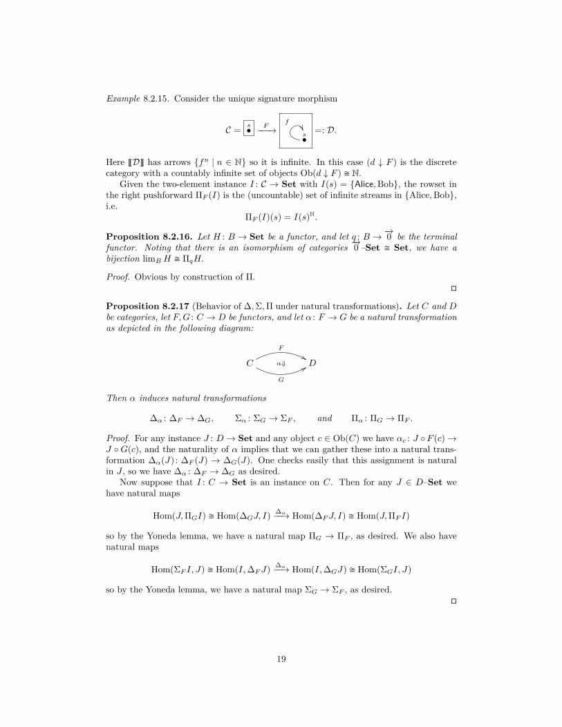
Example 8.2.15. Consider the unique signature morphism

C = s• F−−−→s•

f�� =: D.

Here ~D� has arrows {fn | n ∈ N} so it is infinite. In this case (d ↓ F ) is the discretecategory with a countably infinite set of objects Ob(d ↓ F ) � N.

Given the two-element instance I : C → Set with I(s) = {Alice,Bob}, the rowset inthe right pushforward ΠF (I) is the (uncountable) set of infinite streams in {Alice,Bob},i.e.

ΠF (I)(s) = I(s)N.

Proposition 8.2.16. Let H : B → Set be a functor, and let q : B → −→0 be the terminalfunctor. Noting that there is an isomorphism of categories −→0 –Set � Set, we have abijection limB H � ΠqH.

Proof. Obvious by construction of Π.�

Proposition 8.2.17 (Behavior of ∆,Σ,Π under natural transformations). Let C and Dbe categories, let F,G : C → D be functors, and let α : F → G be a natural transformationas depicted in the following diagram:

C

F

&&

G

88α⇓ D

Then α induces natural transformations

∆α : ∆F → ∆G, Σα : ΣG → ΣF , and Πα : ΠG → ΠF .

Proof. For any instance J : D → Set and any object c ∈ Ob(C) we have αc : J ◦F (c)→J ◦G(c), and the naturality of α implies that we can gather these into a natural trans-formation ∆α(J) : ∆F (J) → ∆G(J). One checks easily that this assignment is naturalin J , so we have ∆α : ∆F → ∆G as desired.

Now suppose that I : C → Set is an instance on C. Then for any J ∈ D–Set wehave natural maps

Hom(J,ΠGI) � Hom(∆GJ, I) ∆α−−→ Hom(∆FJ, I) � Hom(J,ΠF I)

so by the Yoneda lemma, we have a natural map ΠG → ΠF , as desired. We also havenatural maps

Hom(ΣF I, J) � Hom(I,∆FJ) ∆α−−→ Hom(I,∆GJ) � Hom(ΣGI, J)

so by the Yoneda lemma, we have a natural map ΣG → ΣF , as desired.�

19

8.3 Relation to SQL queriesSuppose we are working in a domain DOM ∈ Ob(Set).

Definition 8.3.1. A set-theoretic SQL query q is an expression of the form

SELECT DISTINCT PFROM (c1,1, . . . , c1,k1), . . . , (cn,1, . . . , cn,kn)WHERE W

where n, k1, . . . , kn ∈ N are natural numbers, C is a set of the form C =∐i{ci,1, . . . , ci,ki},

W is a set of pairs W ⊆ C × C, and P : P0 → C is a function, for some set P0.A bag-theoretic SQL query q′ is an expression of the form

SELECT PFROM (c1,1, . . . , c1,k1), . . . , (cn,1, . . . , cn,kn)WHERE W

where n, k1, . . . , kn, C,W,P, P0 are as above. We call (n, k1, . . . , kn, C,W,P, P0) an ag-nostic SQL query.

Suppose that for each 1 ≤ i ≤ n we are given a relation Ri ⊆∏

1≤j≤ki DOM .The evaluation of q (respectively, the evaluation of q′) on R1, . . . , Rn is a relation

Q(R1, . . . , Rn) ⊆∏i∈P0

Ri (respectively, a function Q′(R1, . . . , Rn) : B′ →∏i∈P0

Ri forsome set B′), defined as follows. Let

B′ = {r ∈ R1 × · · · ×Rn | r.c1 = r.c2 for all (c1, c2) ∈W}.

We compose an inclusion with a projection to get a function

B′ ⊆ R1 × · · · ×RnP−→∏i∈P0

Ri.

and defineQ′(R1, . . . , Rn) to be this function. Its image is the desired relationQ(R1, . . . , Rn) ⊆∏i∈P0

Ri.

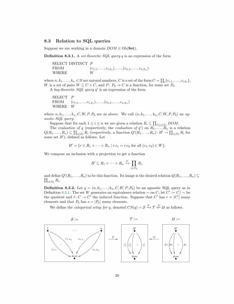
Definition 8.3.2. Let q = (n, k1, . . . , kn, C,W,P, P0) be an agnostic SQL query as inDefinition 8.3.1. The set W generates an equivalence relation ∼ on C; let C ′ := C/ ∼ bethe quotient and ` : C → C ′ the induced function. Suppose that C ′ has r = |C ′| manyelements and that P0 has s = |P0| many elements.

We define the categorical setup for q, denoted CS(q) = S F−→ T G←− U as follows.

S :=

1•

c1,1

((

c1,k1

��

···

· · · n•

cn,1

��cn,kn

vvdom•

F //

T :=

B′•

c′1

��

c′2

��

··· c′r

��dom•

Goo

U :=

B′•

p1

��

p2

��

··· ps

��dom•

20

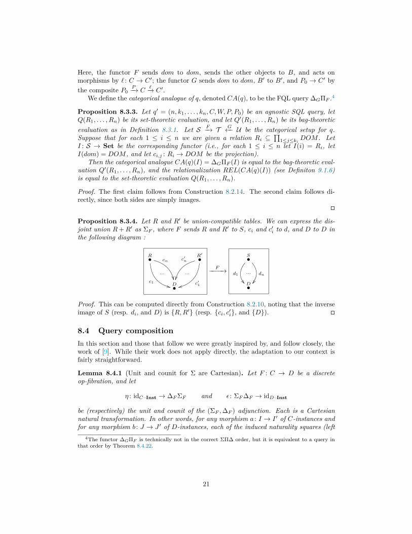
Here, the functor F sends dom to dom, sends the other objects to B, and acts onmorphisms by ` : C → C ′; the functor G sends dom to dom, B′ to B′, and P0 → C ′ bythe composite P0

P−→ C`−→ C ′.

We define the categorical analogue of q, denoted CA(q), to be the FQL query ∆GΠF .4

Proposition 8.3.3. Let q′ = (n, k1, . . . , kn, C,W,P, P0) be an agnostic SQL query, letQ(R1, . . . , Rn) be its set-theoretic evaluation, and let Q′(R1, . . . , Rn) be its bag-theoreticevaluation as in Definition 8.3.1. Let S F−→ T G←− U be the categorical setup for q.Suppose that for each 1 ≤ i ≤ n we are given a relation Ri ⊆

∏1≤j≤ki DOM . Let

I : S → Set be the corresponding functor (i.e., for each 1 ≤ i ≤ n let I(i) = Ri, letI(dom) = DOM , and let ci,j : Ri → DOM be the projection).

Then the categorical analogue CA(q)(I) = ∆GΠF (I) is equal to the bag-theoretic eval-uation Q′(R1, . . . , Rn), and the relationalization REL(CA(q)(I)) (see Definiton 9.1.6)is equal to the set-theoretic evaluation Q(R1, . . . , Rn).

Proof. The first claim follows from Construction 8.2.14. The second claim follows di-rectly, since both sides are simply images.

�

Proposition 8.3.4. Let R and R′ be union-compatible tables. We can express the dis-joint union R+R′ as ΣF , where F sends R and R′ to S, ci and c′i to d, and D to D inthe following diagram :

R•

c1++

···

cn

��

R′•c′n

��···

c′1ssD•

F−−−−→

S•

d1

��··· dn

��D•

Proof. This can be computed directly from Construction 8.2.10, noting that the inverseimage of S (resp. di, and D) is {R,R′} (resp. {ci, c′i}, and {D}). �

8.4 Query compositionIn this section and those that follow we were greatly inspired by, and follow closely, thework of [9]. While their work does not apply directly, the adaptation to our context isfairly straightforward.

Lemma 8.4.1 (Unit and counit for Σ are Cartesian). Let F : C → D be a discreteop-fibration, and let

η : idC–Inst → ∆FΣF and ε : ΣF∆F → idD–Inst

be (respectively) the unit and counit of the (ΣF ,∆F ) adjunction. Each is a Cartesiannatural transformation. In other words, for any morphism a : I → I ′ of C-instances andfor any morphism b : J → J ′ of D-instances, each of the induced naturality squares (left

4The functor ∆GΠF is technically not in the correct ΣΠ∆ order, but it is equivalent to a query inthat order by Theorem 8.4.22.

21

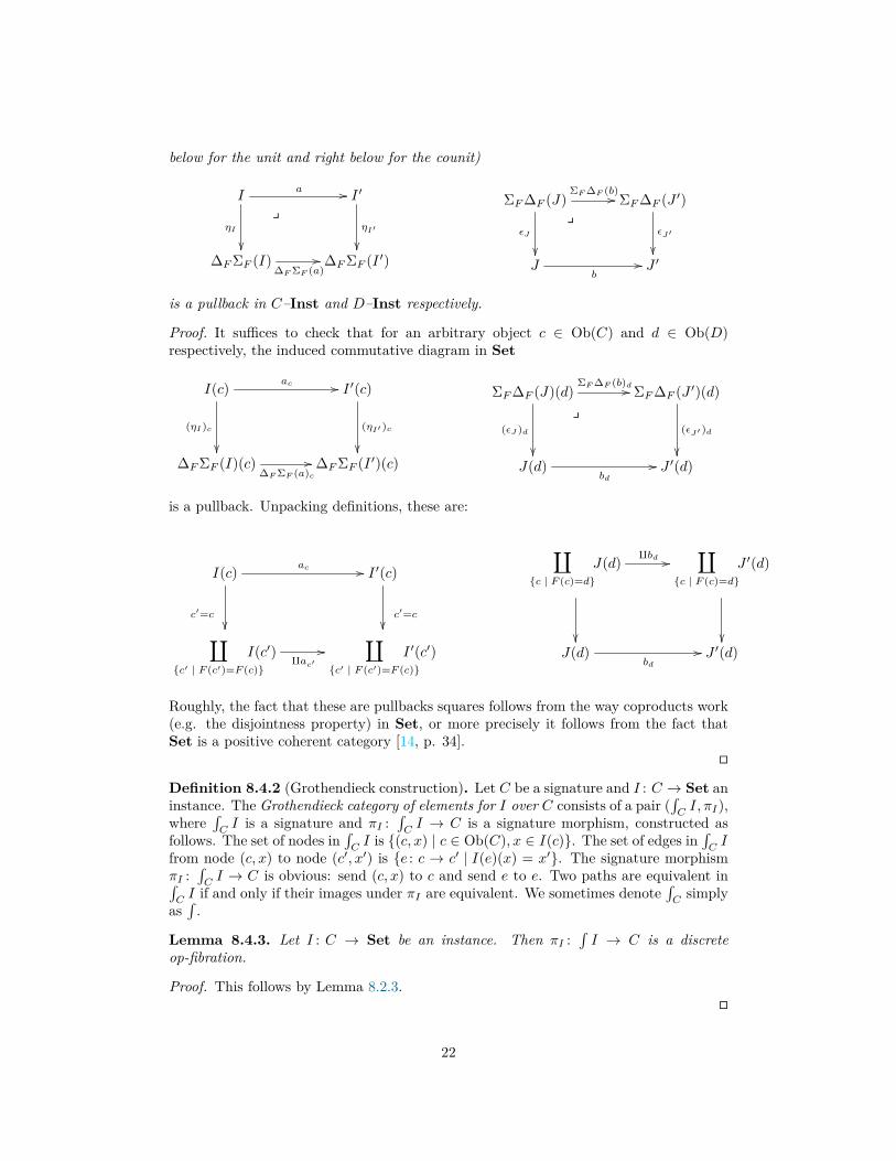
below for the unit and right below for the counit)

Ia //

ηI

��

yI ′

ηI′

��∆FΣF (I)

∆FΣF (a)// ∆FΣF (I ′)

ΣF∆F (J)ΣF∆F (b)//

εJ

��

yΣF∆F (J ′)

εJ′

��J

b// J ′

is a pullback in C–Inst and D–Inst respectively.

Proof. It suffices to check that for an arbitrary object c ∈ Ob(C) and d ∈ Ob(D)respectively, the induced commutative diagram in Set

I(c) ac //

(ηI)c

��

I ′(c)

(ηI′ )c

��∆FΣF (I)(c)

∆FΣF (a)c// ∆FΣF (I ′)(c)

ΣF∆F (J)(d)ΣF∆F (b)d//

(εJ )d

��

y

ΣF∆F (J ′)(d)

(εJ′ )d

��J(d)

bd

// J ′(d)

is a pullback. Unpacking definitions, these are:

I(c) ac //

c′=c��

I ′(c)

c′=c��∐

{c′ | F (c′)=F (c)}I(c′)

qac′//

∐{c′ | F (c′)=F (c)}

I ′(c′)

∐{c | F (c)=d}

J(d) qbd //

��

∐{c | F (c)=d}

J ′(d)

��J(d)

bd

// J ′(d)

Roughly, the fact that these are pullbacks squares follows from the way coproducts work(e.g. the disjointness property) in Set, or more precisely it follows from the fact thatSet is a positive coherent category [14, p. 34].

�

Definition 8.4.2 (Grothendieck construction). Let C be a signature and I : C → Set aninstance. The Grothendieck category of elements for I over C consists of a pair (

∫CI, πI),

where∫CI is a signature and πI :

∫CI → C is a signature morphism, constructed as

follows. The set of nodes in∫CI is {(c, x) | c ∈ Ob(C), x ∈ I(c)}. The set of edges in

∫CI

from node (c, x) to node (c′, x′) is {e : c → c′ | I(e)(x) = x′}. The signature morphismπI :

∫CI → C is obvious: send (c, x) to c and send e to e. Two paths are equivalent in∫

CI if and only if their images under πI are equivalent. We sometimes denote

∫C

simplyas∫

.

Lemma 8.4.3. Let I : C → Set be an instance. Then πI :∫I → C is a discrete

op-fibration.

Proof. This follows by Lemma 8.2.3.�

22

Lemma 8.4.4 (Acyclicity and finiteness are preserved under the Grothendieck construc-tion). Suppose that C is an acyclic (respectively, a finite) signature and that I : C → Setis a finite instance. Then

∫I is an acyclic (respectively, a finite) signature.

Proof. Both are obvious by construction.�

Definition 8.4.5 (DeGrothendieckification). Let π : X → C be a discrete op-fibration.Let {∗}X denote a terminal object in X–Inst, i.e. any instance in which every nodetable and edge table consists of precisely one row. Define the deGrothendieckification ofπ, denoted ∂π : C → Set to be ∂π := Σπ

({∗}X

)∈ C–Inst.

One checks that for a discrete op-fibration π : X → C and object c ∈ Ob(C) we havethe formula

∂π(c) = π−1(c),

so we can say that deGrothendieckification is given by pre-image.

Lemma 8.4.6 (Finiteness is preserved under DeGrothendiekification). If X is a finitesignature and π : X → C is any discrete op-fibration, then ∂π is a finite C-instance.

Proof. Obvious.�

Proposition 8.4.7. Given a signature C, let DopfC ⊆ Cat/C denote the full cat-egory spanned by the discrete op-fibrations over C. Then

∫: C–Inst → DopfC and

∂ : DopfC → C–Inst are functorial, ∂ is left adjoint to∫

, and they are mutually inverseequivalences of categories.

Proof. See [15, Lemma 2.3.4, Proposition 3.2.5].�

Corollary 8.4.8. Suppose that C and D are categories, that F,G : C → D are discreteop-fibrations, and α : F → G is a natural transformation. Then there exists a functorp : C → C such that F ◦ p = G, and Σα = ∂(p), where Σα : ΣG → ΣF is the naturaltransformation given in Proposition 8.2.17.

Proof. By Proposition 8.2.17 the natural transformation α : F → G induces a naturaltransformation ΣG → ΣF , and applying deGrothendieckification supplies a map ∂G →∂F . By Proposition 8.4.7 this induces a map p : C → C over D with the above properties.

�

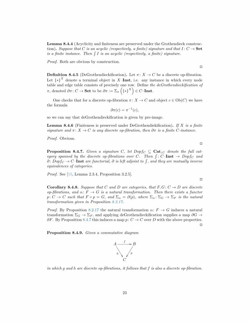
Proposition 8.4.9. Given a commutative diagram

Af //

h��

B

g��

C

in which g and h are discrete op-fibrations, it follows that f is also a discrete op-fibration.

23

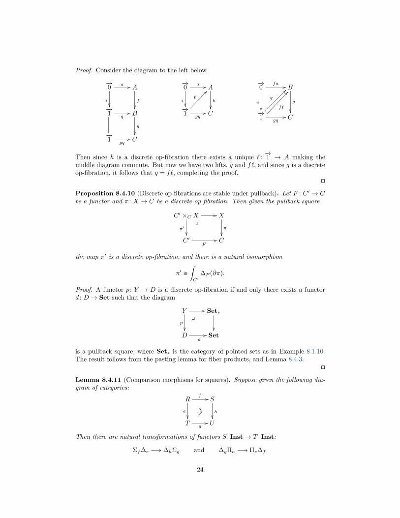
Proof. Consider the diagram to the left below

−→0 a //

i��

A

f

��−→1q// B

g

��−→1gq// C

−→0 a //

i��

A

h

��−→1

`

??

gq// C

−→0 fa //

i

��

B

g

��−→1

q

??

f`

??

gq// C

Then since h is a discrete op-fibration there exists a unique ` : −→1 → A making themiddle diagram commute. But now we have two lifts, q and f`, and since g is a discreteop-fibration, it follows that q = f`, completing the proof.

�

Proposition 8.4.10 (Discrete op-fibrations are stable under pullback). Let F : C ′ → Cbe a functor and π : X → C be a discrete op-fibration. Then given the pullback square

C ′ ×C X //

π′

��

yX

π

��C ′

F// C

the map π′ is a discrete op-fibration, and there is a natural isomorphism

π′ �

∫C′

∆F (∂π).

Proof. A functor p : Y → D is a discrete op-fibration if and only there exists a functord : D → Set such that the diagram

Y //

p

��

ySet∗

��D

d// Set

is a pullback square, where Set∗ is the category of pointed sets as in Example 8.1.10.The result follows from the pasting lemma for fiber products, and Lemma 8.4.3.

�

Lemma 8.4.11 (Comparison morphisms for squares). Suppose given the following dia-gram of categories:

Rf //

e

��

α

t

S

h��

Tg// U

Then there are natural transformations of functors S–Inst→ T–Inst:

Σf∆e −→ ∆hΣg and ∆gΠh −→ Πe∆f .

24

If hf = ge and α = id (i.e. if the diagram commutes) then, by symmetry, there arenatural transformations of functors T–Inst→ S–Inst:

Σe∆f −→ ∆gΣh and ∆hΠg −→ Πf∆e.

Proof. These arise from units and counits, together with Proposition 8.2.17.

Σf∆eηg−→ Σf∆e∆gΣg

∆α−−→ Σf∆f∆hΣgεf−→ ∆hΣg

∆gΠhηe−→ Πe∆e∆gΠh

∆α−−→ Πe∆f∆hΠhεh−→ Πe∆f .

The second claim is symmetric to the first if α = id. �

Definition 8.4.12. Suppose given a diagram of the form

Rf //

e

��

α

t

S

h��

Tg// U

We say it is exact if the comparison morphism Σf∆e → ∆hΣg is an isomorphism. Notethat this is the case if and only if the comparison morphism ∆gΠh → Πe∆f is anisomorphism.

Proposition 8.4.13 (Comma Beck-Chevalley for Σ,∆). Let F : C → D and G : E → Dbe functors, and consider the canonical natural transformation diagram (see Definition8.1.9)

(F ↓ G) q //

p

��

α

t

E

G

��C

F// D

(8)

Let ΣF be the generalized left push-forward as defined in Remark 8.2.12. Then thecomparison morphism (Lemma 8.4.11) is an isomorphism

Σq∆p�−→ ∆GΣF

of functors C–Inst→ E–Inst. In other words, (8) is exact.

Proof. The map is given by the composition

Σq∆pηF // Σq∆p∆FΣF

α // Σq∆q∆GΣFεq // ∆GΣF

To prove it is an isomorphism, one checks it on each object e ∈ Ob(E) by proving that

25

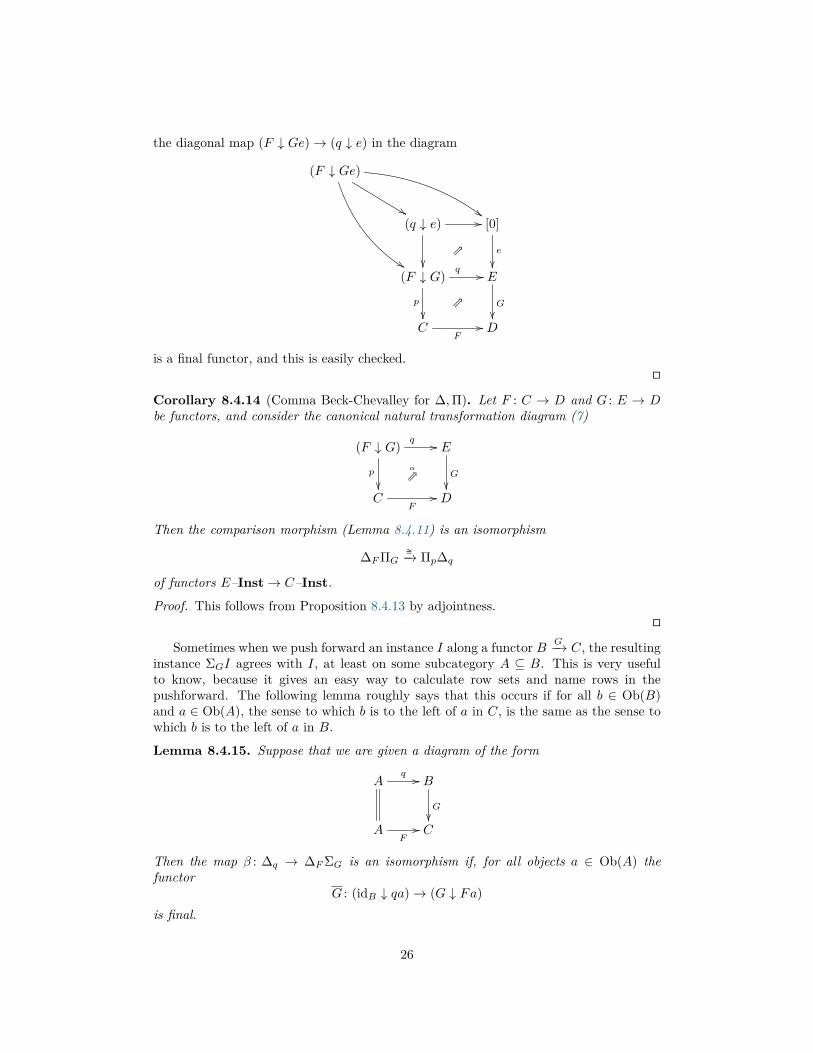
the diagonal map (F ↓ Ge)→ (q ↓ e) in the diagram

(F ↓ Ge)

##%%

%%

(q ↓ e) //

��t

[0]

e

��(F ↓ G)

tp

��

q // E

G

��C

F// D

is a final functor, and this is easily checked.�

Corollary 8.4.14 (Comma Beck-Chevalley for ∆,Π). Let F : C → D and G : E → Dbe functors, and consider the canonical natural transformation diagram (7)

(F ↓ G) q //

p

��

α

t

E

G

��C

F// D

Then the comparison morphism (Lemma 8.4.11) is an isomorphism

∆FΠG�−→ Πp∆q

of functors E–Inst→ C–Inst.

Proof. This follows from Proposition 8.4.13 by adjointness.�

Sometimes when we push forward an instance I along a functor B G−→ C, the resultinginstance ΣGI agrees with I, at least on some subcategory A ⊆ B. This is very usefulto know, because it gives an easy way to calculate row sets and name rows in thepushforward. The following lemma roughly says that this occurs if for all b ∈ Ob(B)and a ∈ Ob(A), the sense to which b is to the left of a in C, is the same as the sense towhich b is to the left of a in B.

Lemma 8.4.15. Suppose that we are given a diagram of the form

Aq // B

G��

AF// C

Then the map β : ∆q → ∆FΣG is an isomorphism if, for all objects a ∈ Ob(A) thefunctor

G : (idB ↓ qa)→ (G ↓ Fa)is final.

26

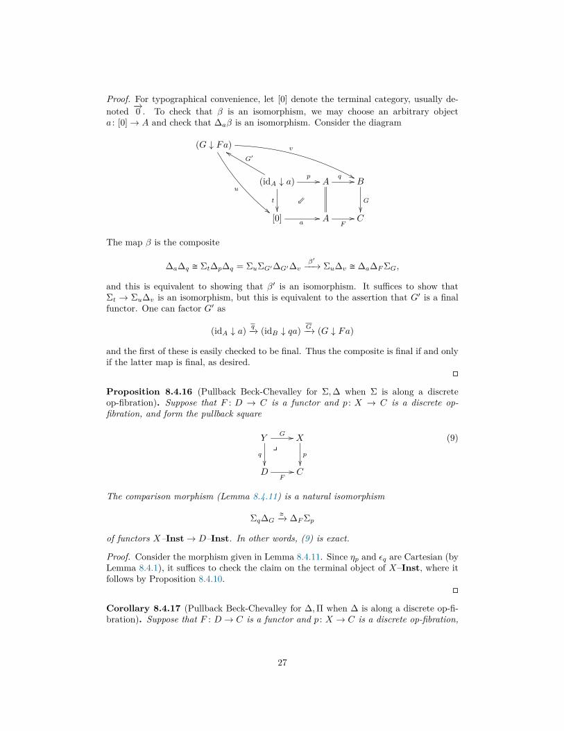
Proof. For typographical convenience, let [0] denote the terminal category, usually de-noted −→0 . To check that β is an isomorphism, we may choose an arbitrary objecta : [0]→ A and check that ∆aβ is an isomorphism. Consider the diagram

(G ↓ Fa) v

&&u

""

(idA ↓ a) p //

t

��

G′ff

w

Aq // B

G

��[0]

a// A

F// C

The map β is the composite

∆a∆q � Σt∆p∆q = ΣuΣG′∆G′∆vβ′−−→ Σu∆v � ∆a∆FΣG,

and this is equivalent to showing that β′ is an isomorphism. It suffices to show thatΣt → Σu∆v is an isomorphism, but this is equivalent to the assertion that G′ is a finalfunctor. One can factor G′ as

(idA ↓ a) q−→ (idB ↓ qa) G−→ (G ↓ Fa)

and the first of these is easily checked to be final. Thus the composite is final if and onlyif the latter map is final, as desired.

�

Proposition 8.4.16 (Pullback Beck-Chevalley for Σ,∆ when Σ is along a discreteop-fibration). Suppose that F : D → C is a functor and p : X → C is a discrete op-fibration, and form the pullback square

Yy

G //

q

��

X

p

��D

F// C

(9)

The comparison morphism (Lemma 8.4.11) is a natural isomorphism

Σq∆G�−→ ∆FΣp

of functors X–Inst→ D–Inst. In other words, (9) is exact.

Proof. Consider the morphism given in Lemma 8.4.11. Since ηp and εq are Cartesian (byLemma 8.4.1), it suffices to check the claim on the terminal object of X–Inst, where itfollows by Proposition 8.4.10.

�

Corollary 8.4.17 (Pullback Beck-Chevalley for ∆,Π when ∆ is along a discrete op-fi-bration). Suppose that F : D → C is a functor and p : X → C is a discrete op-fibration,

27

and form the pullback square

Yy

G //

q

��

X

p

��D

F// C

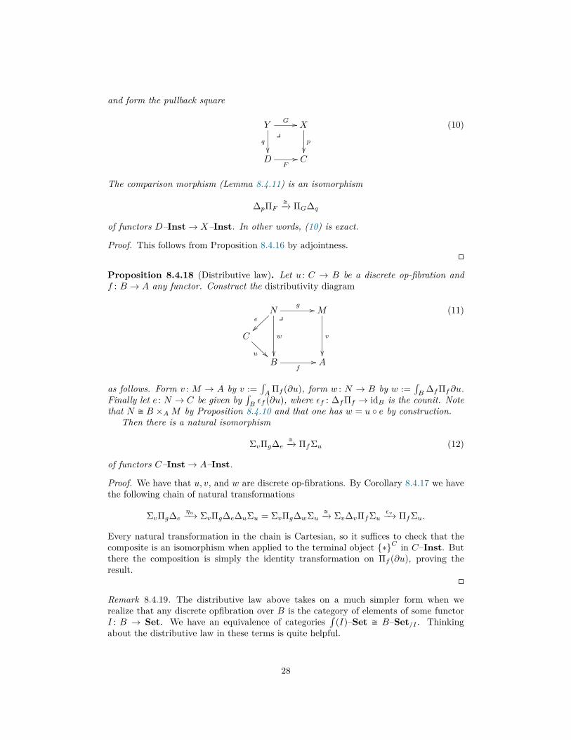
(10)

The comparison morphism (Lemma 8.4.11) is an isomorphism

∆pΠF�−→ ΠG∆q

of functors D–Inst→ X–Inst. In other words, (10) is exact.

Proof. This follows from Proposition 8.4.16 by adjointness.�

Proposition 8.4.18 (Distributive law). Let u : C → B be a discrete op-fibration andf : B → A any functor. Construct the distributivity diagram

Nye

~~

g //

w

��

M

v

��

C

u B

f// A

(11)

as follows. Form v : M → A by v :=∫A

Πf (∂u), form w : N → B by w :=∫B

∆fΠf∂u.Finally let e : N → C be given by

∫Bεf (∂u), where εf : ∆fΠf → idB is the counit. Note

that N � B ×AM by Proposition 8.4.10 and that one has w = u ◦ e by construction.Then there is a natural isomorphism

ΣvΠg∆e�−→ ΠfΣu (12)

of functors C–Inst→ A–Inst.

Proof. We have that u, v, and w are discrete op-fibrations. By Corollary 8.4.17 we havethe following chain of natural transformations

ΣvΠg∆eηu−→ ΣvΠg∆e∆uΣu = ΣvΠg∆wΣu

�−→ Σv∆vΠfΣuεv−→ ΠfΣu.

Every natural transformation in the chain is Cartesian, so it suffices to check that thecomposite is an isomorphism when applied to the terminal object {∗}C in C–Inst. Butthere the composition is simply the identity transformation on Πf (∂u), proving theresult.

�

Remark 8.4.19. The distributive law above takes on a much simpler form when werealize that any discrete opfibration over B is the category of elements of some functorI : B → Set. We have an equivalence of categories

∫(I)–Set � B–Set/I . Thinking

about the distributive law in these terms is quite helpful.

28

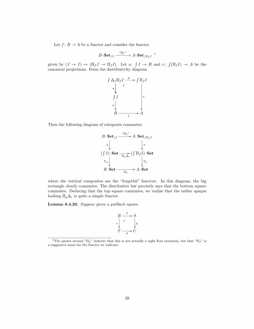
Let f : B → A be a functor and consider the functor

B–Set/I“Πf”−−−−−→ A–Set/Πf I 5

given by (J → I) 7→ (ΠfJ → ΠfI). Let u :∫I → B and v :

∫(ΠfI) → A be the

canonical projections. Form the distributivity diagram∫∆fΠfI

ye

��

g //

e

��

∫ΠfI

v

��

∫I

u

��B

f// A

Then the following diagram of categories commutes:

B–Set/I“Πf” //

�

��

A–Set/Πf I

�

��(∫I)–Set

Πg∆e

//

Σu��

(∫

ΠfI)–Set

Σv��

B–SetΠf

// A–Set

where the vertical composites are the “forgetful” functors. In this diagram, the bigrectangle clearly commutes. The distributive law precisely says that the bottom squarecommutes. Deducing that the top square commutes, we realize that the rather opaquelooking Πg∆e is quite a simple functor.

Lemma 8.4.20. Suppose given a pullback square.

Ry

f //

e

��

S

h��

Tg// U

5The quotes around “Πf” indicate that this is not actually a right Kan extension, but that “Πf” isa suggestive name for the functor we indicate.

29

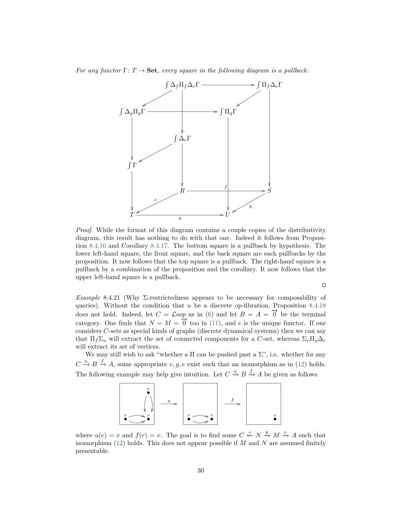
For any functor Γ: T → Set, every square in the following diagram is a pullback:∫∆fΠf∆eΓ

��

//

xx

∫Πf∆eΓ

��

yy∫∆gΠgΓ

��

//∫

ΠgΓ

��

∫∆eΓ

��

xx∫Γ

��

Rf //

e

ww

S

hxx

Tg

// U

Proof. While the format of this diagram contains a couple copies of the distributivitydiagram, this result has nothing to do with that one. Indeed it follows from Proposi-tion 8.4.10 and Corollary 8.4.17. The bottom square is a pullback by hypothesis. Thelower left-hand square, the front square, and the back square are each pullbacks by theproposition. It now follows that the top square is a pullback. The right-hand square is apullback by a combination of the proposition and the corollary. It now follows that theupper left-hand square is a pullback.

�

Example 8.4.21 (Why Σ-restrictedness appears to be necessary for composability ofqueries). Without the condition that u be a discrete op-fibration, Proposition 8.4.18does not hold. Indeed, let C = Loop as in (6) and let B = A = −→0 be the terminalcategory. One finds that N = M = −→0 too in (11), and e is the unique functor. If oneconsiders C-sets as special kinds of graphs (discrete dynamical systems) then we can saythat ΠfΣu will extract the set of connected components for a C-set, whereas ΣvΠg∆e

will extract its set of vertices.We may still wish to ask “whether a Π can be pushed past a Σ”, i.e. whether for any

Cu−→ B

f−→ A, some appropriate v, g, e exist such that an isomorphism as in (12) holds.The following example may help give intuition. Let C u−→ B

f−→ A be given as follows

e•

�� ��r• ((

66v•

u //

e•

r• ((66v•

f //

e•

r• v•

where u(e) = v and f(r) = v. The goal is to find some C e←− Ng−→ M

v−→ A such thatisomorphism (12) holds. This does not appear possible if M and N are assumed finitelypresentable.

30

Theorem 8.4.22 (Query composition). Suppose that one has Σ-restricted data migra-tion queries Q : S { T and Q′ : T { U as follows:

Bf //

s

��

A

t

��

Dg //

u

��

C

v

��S Q T T Q′ U

(13)

Then there exists a Σ-restricted data migration query Q′′ : S { U such that ~Q′′� �~Q′� ◦ ~Q�.Proof. We follow the proof in [9], as we have been throughout this section. We will formQ′′ by constructing the following diagram, which we will explain step by step:

Np //

n

~~(iv)

D′q //

e~~(ii)

M

w

��

B′r //

m

~~(iii)

A′

k

h

~~(i)B

s

��

f // A

t

D

u}}

g // Cv

S T U

(14)

First, form (i) by taking the pullback; note that k is a discrete op-fibration by Proposition8.4.10. Second, form (ii) as a distributivity diagram (see Proposition 8.4.18) and notethat w is a discrete op-fibration. Third, form (iii) and (iv) with B′ = (f ↓ h) andN = (r ↓ e).

By Proposition 8.4.16 we have ∆uΣt � Σk∆h. By Proposition 8.4.18 we have ΠgΣk �ΣwΠq∆e. By Corollary 8.4.14 we have both ∆hΠf � Πr∆m and ∆eΠr � Πp∆n. Pullingthis all together, we have an isomorphism

ΣvΠg∆uΣtΠf∆s � ΣvΠgΣk∆hΠf∆s � ΣvΣwΠq∆e∆hΠf∆s

� ΣvΣwΠq∆eΠr∆m∆s

� ΣvΣwΠqΠp∆n∆m∆s,

which proves that ~Q′′� � ~Q′� ◦ ~Q�, where Q′′ is the data migration functor given bythe triple of morphisms Q′ := (s ◦ m ◦ n, q ◦ p, v ◦ w), i.e. ~Q� = ΣvwΠqp∆smn. Thiscompletes the proof.

�

Corollary 8.4.23. Suppose that Q : S { T and Q′ : T { U are queries as in (13)and that both are (∆,Σ)-restricted. Then there exists a (∆,Σ)-restricted data migrationquery Q′′ : S { U such that ~Q′′� � ~Q′� ◦ ~Q�.Proof. We form a diagram similar to (14), as follows. First, form (i) by taking thepullback; note that k is a discrete op-fibration by Proposition 8.4.10. Second, form (ii)as a distributivity diagram (see Proposition 8.4.18) and note that w is a discrete op-fibration. Third, form (iii) and (iv) as pullbacks. Note that h, m, and n will be discreteopfibrations. Following the proof of Theorem 8.4.22, the result follows by Corollary8.4.17 in place of Corollary 8.4.14.

�

31

8.5 Syntactic characterization of query morphism and query equiv-alence

We continue to closely follow [9].

Definition 8.5.1 (Morphism of data migration queries). A morphism of (∆,Σ)-restricteddata migration queries from P = (u, g, v) to Q = (s, f, t), denoted (c, a, β) : P → Q, con-sists of two functors c, a and a natural transformation β, fitting into a diagram of theform

P : S Duoo g // C

v // T

B ×A C

β⇑a

OO

f ′ //

b

��

y

C

c

��Q : S B

soo

f// A

t// T

(15)

where blue arrows (u, v, s, t, c) are required to be discrete op-fibrations and every squarecommutes except for the top middle square in which β : f ′ → ga is a natural transfor-mation.

Note that for any diagram of the form (15), the maps a and b will automatically bediscrete op-fibrations too.Remark 8.5.2. Note that a morphism of queries P → Q involves a “backward” morphismsof schemas, a : B ×A C → D as in (15). In fact, this reversal happens in the conjunctivefragment only (see Lemma 8.5.9). This may not be surprising because a is a morphismof indexing categories, or “bound variables”, and thus the directionality is in line withclassical database theory.

Definition 8.5.3 (Composition of data migration queries). Suppose given data migra-tion queries P,Q,R : S { T and morphisms P → Q and Q → R as in Definition 15.Then they can be composed to give a query morphism P → R, as follows.

We begin the following diagram

S Fwoo h //

⇑

Ex // T

D ×C E

OO

//

��

yE

e

��S D

⇑

g //uoo Cv // T

B ×A Cf ′ //

b

��

a

OO

yC

c

��S B

f//

soo A

t// T

32

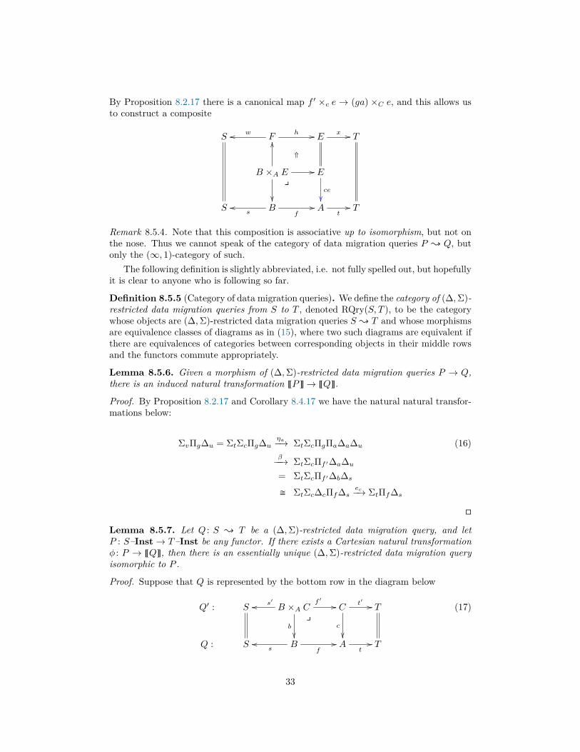
By Proposition 8.2.17 there is a canonical map f ′ ×c e → (ga) ×C e, and this allows usto construct a composite

S Fwoo h //

⇑

Ex // T

B ×A E //

��

OO

yE

ce

��S B

f//

soo A

t// T

Remark 8.5.4. Note that this composition is associative up to isomorphism, but not onthe nose. Thus we cannot speak of the category of data migration queries P { Q, butonly the (∞, 1)-category of such.

The following definition is slightly abbreviated, i.e. not fully spelled out, but hopefullyit is clear to anyone who is following so far.

Definition 8.5.5 (Category of data migration queries). We define the category of (∆,Σ)-restricted data migration queries from S to T , denoted RQry(S, T ), to be the categorywhose objects are (∆,Σ)-restricted data migration queries S { T and whose morphismsare equivalence classes of diagrams as in (15), where two such diagrams are equivalent ifthere are equivalences of categories between corresponding objects in their middle rowsand the functors commute appropriately.

Lemma 8.5.6. Given a morphism of (∆,Σ)-restricted data migration queries P → Q,there is an induced natural transformation ~P�→ ~Q�.

Proof. By Proposition 8.2.17 and Corollary 8.4.17 we have the natural natural transfor-mations below:

ΣvΠg∆u = ΣtΣcΠg∆uηa−→ ΣtΣcΠgΠa∆a∆u (16)β−−→ ΣtΣcΠf ′∆a∆u

= ΣtΣcΠf ′∆b∆s

� ΣtΣc∆cΠf∆sec−→ ΣtΠf∆s

�

Lemma 8.5.7. Let Q : S { T be a (∆,Σ)-restricted data migration query, and letP : S–Inst→ T–Inst be any functor. If there exists a Cartesian natural transformationφ : P → ~Q�, then there is an essentially unique (∆,Σ)-restricted data migration queryisomorphic to P .

Proof. Suppose that Q is represented by the bottom row in the diagram below

Q′ : S B ×A Cs′oo f ′ //

b

��

yC

t′ //

c

��

T

Q : S Bs

oof

// At// T

(17)

33

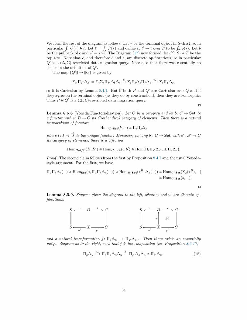
We form the rest of the diagram as follows. Let ∗ be the terminal object in S–Inst, so inparticular

∫TQ(∗) � t. Let t′ =

∫TP (∗) and define c : t′ → t over T to be

∫Tφ(∗). Let b

be the pullback of c and s′ = s ◦ b. The Diagram (17) now formed, let Q′ : S { T be thetop row. Note that c, and therefore b and s, are discrete op-fibrations, so in particularQ′ is a (∆,Σ)-restricted data migration query. Note also that there was essentially nochoice in the definition of Q′.

The map ~Q′�→ ~Q� is given by

Σt′Πf ′∆s′ = ΣtΣcΠf ′∆b∆s�−→ ΣtΣc∆cΠf∆s

ηc−→ ΣtΠf∆s,

so it is Cartesian by Lemma 8.4.1. But if both P and Q′ are Cartesian over Q and ifthey agree on the terminal object (as they do by construction), then they are isomorphic.Thus P � Q′ is a (∆,Σ)-restricted data migration query.

�

Lemma 8.5.8 (Yoneda Functorialization). Let C be a category and let b : C → Set bea functor with s : B → C its Grothendieck category of elements. Then there is a naturalisomorphism of functors

HomC–Set(b,−) � ΠtΠs∆s

where t : I → −→0 is the unique functor. Moreover, for any b′ : C → Set with s′ : B′ → Cits category of elements, there is a bijection

HomCat/C(B,B′) � HomC–Set(b, b′) � Hom(ΠtΠs′∆s′ ,ΠtΠs∆s).

Proof. The second claim follows from the first by Proposition 8.4.7 and the usual Yoneda-style argument. For the first, we have

ΠuΠs∆s(−) � HomSet(∗,ΠuΠs∆s(−)) � HomB–Set(∗B ,∆s(−)) � HomC–Set(Σs(∗B),−)� HomC–Set(b,−).

�

Lemma 8.5.9. Suppose given the diagram to the left, where u and u′ are discrete op-fibrations:

S Duoo g // C

S Xu′

oog′// C

S Duoo g //

β⇑

C

S X

a

OO

u′oo

g′// C

and a natural transformation j : Πg∆u → Πg′∆u′ . Then there exists an essentiallyunique diagram as to the right, such that j is the composition (see Proposition 8.2.17),

Πg∆uηa−→ ΠgΠa∆a∆u

β−→ Πg′∆a∆u � Πg′∆u′ . (18)

34

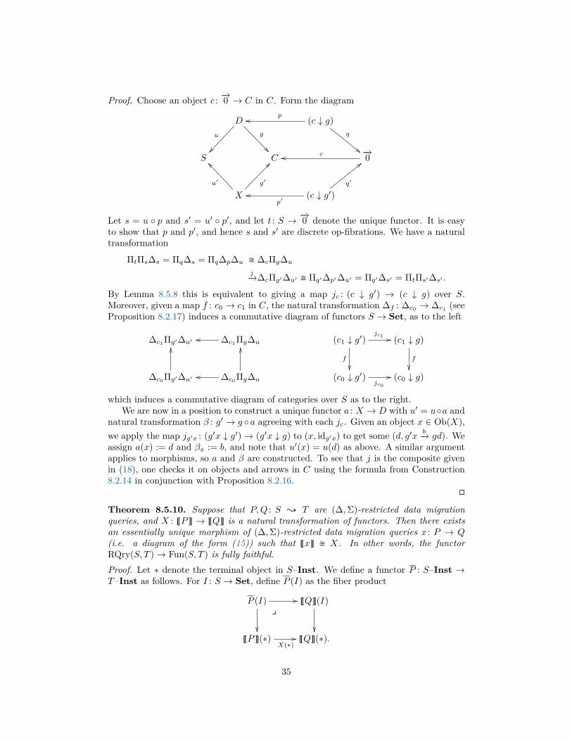
Proof. Choose an object c : −→0 → C in C. Form the diagram

D

u

��

g

��

(c ↓ g)poo

q

""S C

−→0coo

X

u′

^^

g′

@@

(c ↓ g′)p′

ooq′

<<

Let s = u ◦ p and s′ = u′ ◦ p′, and let t : S → −→0 denote the unique functor. It is easyto show that p and p′, and hence s and s′ are discrete op-fibrations. We have a naturaltransformation

ΠtΠs∆s = Πq∆s = Πq∆p∆u � ∆cΠg∆u

j−→∆cΠg′∆u′ � Πq′∆p′∆u′ = Πq′∆s′ = ΠtΠs′∆s′ .

By Lemma 8.5.8 this is equivalent to giving a map jc : (c ↓ g′) → (c ↓ g) over S.Moreover, given a map f : c0 → c1 in C, the natural transformation ∆f : ∆c0 → ∆c1 (seeProposition 8.2.17) induces a commutative diagram of functors S → Set, as to the left

∆c1Πg′∆u′ ∆c1Πg∆uoo

∆c0Πg′∆u′

OO

∆c0Πg∆u

OO

oo

(c1 ↓ g′)jc1 //

f

��

(c1 ↓ g)

f

��(c0 ↓ g′)

jc0

// (c0 ↓ g)

which induces a commutative diagram of categories over S as to the right.We are now in a position to construct a unique functor a : X → D with u′ = u◦a and

natural transformation β : g′ → g ◦ a agreeing with each jc. Given an object x ∈ Ob(X),we apply the map jg′x : (g′x ↓ g′)→ (g′x ↓ g) to (x, idg′x) to get some (d, g′x b−→ gd). Weassign a(x) := d and βx := b, and note that u′(x) = u(d) as above. A similar argumentapplies to morphisms, so a and β are constructed. To see that j is the composite givenin (18), one checks it on objects and arrows in C using the formula from Construction8.2.14 in conjunction with Proposition 8.2.16.

�

Theorem 8.5.10. Suppose that P,Q : S { T are (∆,Σ)-restricted data migrationqueries, and X : ~P� → ~Q� is a natural transformation of functors. Then there existsan essentially unique morphism of (∆,Σ)-restricted data migration queries x : P → Q(i.e. a diagram of the form (15)) such that ~x� � X. In other words, the functorRQry(S, T )→ Fun(S, T ) is fully faithful.Proof. Let ∗ denote the terminal object in S–Inst. We define a functor P : S–Inst →T–Inst as follows. For I : S → Set, define P (I) as the fiber product

P (I) //

��

y~Q�(I)

��~P�(∗)

X(∗)// ~Q�(∗).

35

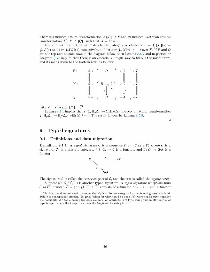
There is a induced natural transformation i : ~P�→ P and an induced Cartesian naturaltransformation X ′ : P → ~Q�, such that X = X ′ ◦ i.

Let v : C → T and t : A → T denote the category of elements v :=∫T~P�(∗) =∫

TP (∗) and t :=

∫T~Q�(∗) respectively, and let c :=

∫TX(∗) : v → t over T . If P and Q

are the top and bottom rows in the diagram below, then Lemma 8.5.7 and in particularDiagram (17) implies that there is an essentially unique way to fill out the middle row,and its maps down to the bottom row, as follows:

P : S Duoo g // C

v // T

P ′ : S B ×A Cs′oo f ′ //

b

��

yC

c

��

v // T

Q : S Bs

oof

// At// T

with s′ = s ◦ b and ~P ′� = P .Lemma 8.4.1 implies that i : ΣvΠg∆u → ΣvΠf ′∆s′ induces a natural transformation

j : Πg∆u → Πf ′∆s′ with Σvj = i. The result follows by Lemma 8.5.9.�

9 Typed signatures9.1 Definitions and data migrationDefinition 9.1.1. A typed signature C is a sequence C := (C, C0, i,Γ) where C is asignature, C0 is a discrete category, 6 i : C0 → C is a functor, and Γ: C0 → Set is afunctor,

C0i //

Γ !!

C

Set

The signature C is called the structure part of C, and the rest is called the typing setup.Suppose (C′, C0,′ i′,Γ′) is another typed signature. A typed signature morphism from

C to C′, denoted F = (F, F0) : C → C′, consists of a functor F : C → C′ and a functor6In fact, one does not need to assume that C0 is a discrete category for the following results to hold.

Still, it is conceptually simpler. To get a feeling for what could be done if C0 were not discrete, considerthe possibility of a table having two data columns, an attribute A of type string and an attribute B oftype integer, where the integer in B was the length of the string in A.

36

F0 : C0 → C′0 such that the following diagram commutes:

C0i //

Γ !!F0

��

C

F

��

Set

C′0

Γ′==

i′// C′

The category of typed signatures is denoted TSig.A C-instance I is a pair I := (I, δ) where I : C → Set is a functor, called the structure

part of I together with a natural transformation δ : I ◦ i→ Γ, called the data part of I.

C0i //

Γ !!

δ⇐

C

I~~Set

Suppose I ′ := (I ′, δ′) is another C-instance. An instance morphism from I to I ′, denotedα : I → I ′, is a natural transformation α : I → I ′ such that δ′ ◦ α = δ.

C0i //

Γ !!

δ′⇐

C

Ixx

α⇐I′

��Set

The category of C-instances is denoted C–Inst.

Proposition 9.1.2. Let C be a typed signature. Then the category C–Inst is a topos.

Proof. C–Inst is equivalent to the slice topos C–Set/ΠiΓ.�

Construction 9.1.3. Let C := (C, C0, i,Γ) be a typed signature. We set up the tablesfor it as follows. For every arrow in C we make a binary table; we call these arrow tables.For every object c ∈ Ob(C), let N = i−1(c) ⊆ C0. We make an 1 + |N | column table,where |N | is the cardinality of N ; we call these node tables. For each node table, onecolumn is the primary key column and the other N columns are called data columns.The data type for each n ∈ N is the set Γ(n).

Let (I, δ) be an instance of C. For each object c ∈ Ob(C) we fill in the primary keycolumn of the node table with the set I(c) ∈ Ob(Set). For each data column n ∈ N wehave a function δn : I(c) → Γ(n), which we use to fill in the data in that column. Forevery arrow f : c → c′ in C we fill in the primary key column of the arrow table withI(c), and we fill in the other column with the function I(f) : I(c)→ I(c′).

Example 9.1.4. If C0 = ∅ then for any category presentation C there is a unique functori : C0 → C and a unique functor Γ: C0 → Set, so there is a unique schema C = (C, ∅, i,Γ)with structure C and empty domain setup.

Given a functor I : C → Set, there is a unique instance I := (I, !) ∈ C–Inst with thatstructure part. The data part of I is empty.

37

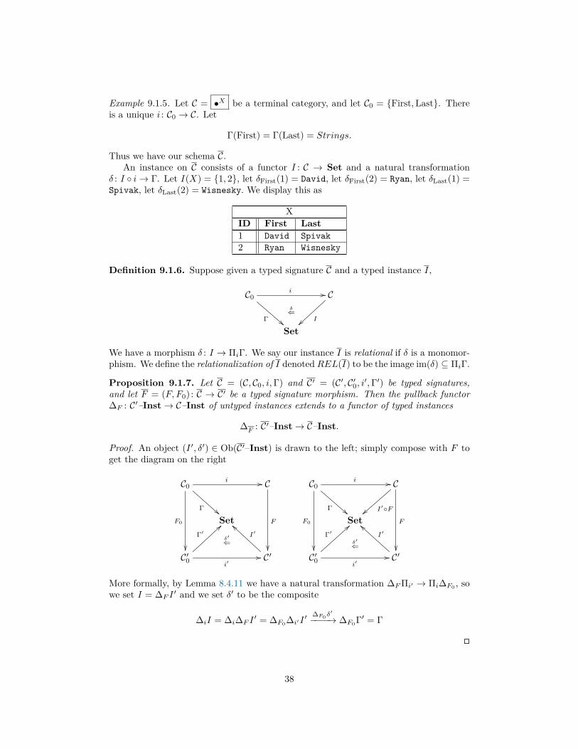
Example 9.1.5. Let C = •X be a terminal category, and let C0 = {First,Last}. Thereis a unique i : C0 → C. Let

Γ(First) = Γ(Last) = Strings.

Thus we have our schema C.An instance on C consists of a functor I : C → Set and a natural transformation

δ : I ◦ i→ Γ. Let I(X) = {1, 2}, let δFirst(1) = David, let δFirst(2) = Ryan, let δLast(1) =Spivak, let δLast(2) = Wisnesky. We display this as

XID First Last1 David Spivak2 Ryan Wisnesky

Definition 9.1.6. Suppose given a typed signature C and a typed instance I,

C0i //

Γ !!

δ⇐

C

I~~Set

We have a morphism δ : I → ΠiΓ. We say our instance I is relational if δ is a monomor-phism. We define the relationalization of I denotedREL(I) to be the image im(δ) ⊆ ΠiΓ.

Proposition 9.1.7. Let C = (C, C0, i,Γ) and C′ = (C′, C′0, i′,Γ′) be typed signatures,and let F = (F, F0) : C → C′ be a typed signature morphism. Then the pullback functor∆F : C′–Inst→ C–Inst of untyped instances extends to a functor of typed instances

∆F : C′–Inst→ C–Inst.

Proof. An object (I ′, δ′) ∈ Ob(C′–Inst) is drawn to the left; simply compose with F toget the diagram on the right

C0i //

Γ !!F0

��

C

F

��

Set

C′0

Γ′==

i′//

δ′⇐

C′

I′``

C0i //

Γ !!F0

��

C

F

��

I′◦F}}Set

C′0

Γ′==

i′//

δ′⇐

C′

I′``

More formally, by Lemma 8.4.11 we have a natural transformation ∆FΠi′ → Πi∆F0 , sowe set I = ∆F I

′ and we set δ′ to be the composite

∆iI = ∆i∆F I′ = ∆F0∆i′I

′ ∆F0δ′

−−−−→ ∆F0Γ′ = Γ

�

38

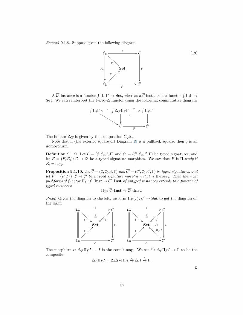
Remark 9.1.8. Suppose given the following diagram:

C0i //

Γ !!F0

��

C

F

��

Set

C′0

Γ′==

i′// C′

(19)

A C′-instance is a functor∫

Πi′Γ′ → Set, whereas a C instance is a functor∫

ΠiΓ→Set. We can reinterpret the typed-∆ functor using the following commutative diagram∫

ΠiΓ

%%

∫∆FΠi′Γ′

qoo

��

r //y

∫Πi′Γ′

��C

F// C′

The functor ∆F is given by the composition Σq∆r.Note that if (the exterior square of) Diagram 19 is a pullback square, then q is an

isomorphism.

Definition 9.1.9. Let C = (C, C0, i,Γ) and C′ = (C′, C0, i′,Γ) be typed signatures, andlet F = (F, F0) : C → C′ be a typed signature morphism. We say that F is Π-ready ifF0 = idC0 .

Proposition 9.1.10. Let C = (C, C0, i,Γ) and C′ = (C′, C0, i′,Γ) be typed signatures, andlet F = (F, F0) : C → C′ be a typed signature morphism that is Π-ready. Then the rightpushforward functor ΠF : C–Inst→ C′–Inst of untyped instances extends to a functor oftyped instances

ΠF : C–Inst→ C′–Inst.

Proof. Given the diagram to the left, we form ΠF (I) : C′ → Set to get the diagram onthe right:

C0i //

Γ !!

δ⇐

C

F

��

I}}Set

C0

Γ==

i′// C′

C0i //

Γ !!

δ⇐

C

F

��

I}}Set ε⇑

C0

Γ==

i′// C′

ΠF Iaa

The morphism ε : ∆FΠF I → I is the counit map. We set δ′ : ∆i′ΠF I → Γ to be thecomposite

∆i′ΠF I = ∆i∆FΠF Iε−→ ∆iI

δ−→ Γ.

�

39

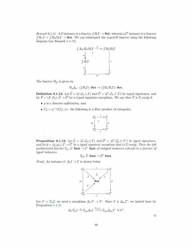
Remark 9.1.11. A C-instance is a functor∫

ΠiΓ→ Set, whereas a C′ instance is a functor∫Πi′Γ =

∫ΠFΠiΓ → Set. We can reinterpret the typed-Π functor using the following

diagram (see Remark 8.4.19).∫∆FΠFΠiΓ

ye

��

g //

e

��

∫ΠFΠiΓ

v

��

∫ΠiΓ

u

��C

F// C′

The functor ΠF is given by

Πg∆e : (∫

ΠiΓ)–Set→ (∫

ΠFΠiΓ)–Set.

Definition 9.1.12. Let C = (C, C0, i,Γ) and C′ = (C′, C0, i′,Γ) be typed signatures, andlet F = (F, F0) : C → C′ be a typed signature morphism. We say that F is Σ-ready if

• p is a discrete opfibration, and

• C0 = p−1(C ′0), i.e. the following is a fiber product of categories,

C0i //

p0

��

yC

p

��C′0

i′// C′

.

Proposition 9.1.13. Let C = (C, C0, i,Γ) and C′ = (C′, C′0, i′,Γ′) be typed signatures,and let p = (p, p0) : C → C′ be a typed signature morphism that is Σ-ready. Then the leftpushforward functor Σp : C–Inst→ C′–Inst of untyped instances extends to a functor oftyped instances

Σp : C–Inst→ C′–Inst.

Proof. An instance δ : ∆iI → Γ is drawn below

C0i //

Γ !!p0

��

δ⇐

C

p

��

I}}Set

C′0

Γ′==

i′// C′

Let I ′ = ΣpI; we need a morphism ∆i′I′ → Γ′. Since Γ � ∆p0Γ′, we indeed have by

Proposition 8.4.16∆i′ΣpI

�−→ Σp0∆iIΣp0δ−−−→ Σp0∆p0Γ′ ε−→ Γ′.

�

40

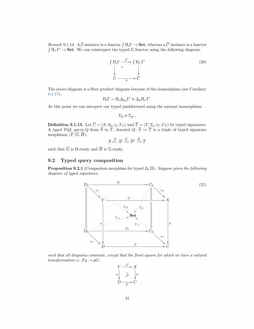
Remark 9.1.14. A C-instance is a functor∫

ΠiΓ→ Set, whereas a C′ instance is a functor∫Πi′Γ′ → Set. We can reinterpret the typed-Σ functor using the following diagram.

∫ΠiΓy

��

p′ //∫

Πi′Γ′

��C

p// C′

(20)

The above diagram is a fiber product diagram because of the isomorphism (see Corollary8.4.17):

ΠiΓ = Πi∆p0Γ′ � ∆pΠi′Γ′.

At this point we can interpret our typed pushforward using the natural isomorphism

Σp � Σp′ .

Definition 9.1.15. Let C = (S, S0, iS ,ΓS) and T = (T, T0, iT ,ΓT ) be typed signatures.A typed FQL query Q from S to T , denoted Q : S { T is a triple of typed signaturemorphisms (F ,G,H):

SF←− S′ G−→ S′′

H−→ T

such that G is Π-ready and H is Σ-ready.

9.2 Typed query compositionProposition 9.2.1 (Comparison morphism for typed ∆,Π). Suppose given the followingdiagram of typed signatures,

D0

ΓD$$

F0 //

iY

C0

ΓC��

iX

Y

G //

q

��

X

p

��

Set

D0

ΓD 44

F0 //

iD

C0

ΓC

aa

iC

D

F // C

(21)

such that all diagrams commute, except that the front square for which we have a naturaltransformation α : Fq → pG:

YG //

q

��

α

t

X

p

��D

F// C

41

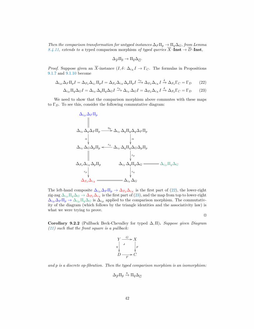
Then the comparison transformation for untyped instances ∆FΠp → Πq∆G, from Lemma8.4.11, extends to a typed comparison morphism of typed queries X–Inst→ D–Inst,

∆FΠp → Πq∆G.

Proof. Suppose given an X-instance (I, δ : ∆iX I → ΓC . The formulas in Propositions9.1.7 and 9.1.10 become

∆iD∆FΠpI = ∆F0∆iCΠpI = ∆F0∆iX∆pΠpIεp−→ ∆F0∆iX I

δ−→ ∆F0ΓC = ΓD (22)

∆iDΠq∆GI = ∆iY ∆qΠq∆GIεq−→ ∆iY ∆GI = ∆F0∆iX I

δ−→ ∆F0ΓC = ΓD (23)

We need to show that the comparison morphism above commutes with these mapsto ΓD. To see this, consider the following commutative diagram:

∆iD∆FΠp

∆iY ∆q∆FΠp

α

��

ηq // ∆iY ∆qΠq∆q∆FΠp

α

��∆iY ∆G∆pΠp ∆iY ∆qΠq∆G∆pΠp

εqoo

εp

��∆F0∆iX∆pΠp

εp

��

∆iY ∆qΠq∆G

εq

��

∆iDΠq∆G

∆F0∆iX ∆iY ∆G

The left-hand composite ∆iD∆FΠp → ∆F0∆iX is the first part of (22), the lower-rightzig-zag ∆iDΠq∆G → ∆F0∆iX is the first part of (23), and the map from top to lower-right∆iD∆FΠp → ∆iDΠq∆G is ∆iD applied to the comparison morphism. The commutativ-ity of the diagram (which follows by the triangle identities and the associativity law) iswhat we were trying to prove.

�

Corollary 9.2.2 (Pullback Beck-Chevalley for typed ∆,Π). Suppose given Diagram(21) such that the front square is a pullback:

YG //

q

��

yX

p

��D

F// C

and p is a discrete op-fibration. Then the typed comparison morphism is an isomorphism:

∆FΠp�−→ Πq∆G

42

Proof. By Corollary 8.4.17, the comparison morphism is an isomorphism,

∆FΠp�−→ Πq∆G.

The result follows from Proposition 9.2.1, where iY : D0 → Y is induced by the fact thatY is a fiber product.

�

Corollary 9.2.3 (Comma Beck-Chevalley for typed ∆,Π). Suppose given Diagram (21)such that the front square is a comma category:

Y = (F ↓ p) G //

q

��

α

t

X

p

��D

F// C

Then the typed comparison morphism is an isomorphism:

∆FΠp�−→ Πq∆G

Proof. By Corollary 8.4.14, the comparison morphism is an isomorphism,

∆FΠp�−→ Πq∆G.

The result follows from Proposition 9.2.1, where iY : D0 → Y is the induced map factor-ing through the canonical morphism F ×C p→ (F ↓ p).

�

Proposition 9.2.4 (Pullback Beck-Chevalley for typed Σ,∆). Suppose given the fol-lowing commutative diagram of typed signatures,

Y0

ΓY$$

G0 //

iY

q0

��

X0

ΓX��

p0

��

iX

Y

G //

q

��

X

p

��

Set

D0

ΓD 44

F0 //

iD

C0

ΓC

aa

iC

D

F // C

in which p : X → C is a discrete op-fibration, and the four side squares

Y0iY //

q0

��

yY

q

��D0

iD// D

Y0G0 //

q0

��

yX0

p0

��D0

F0

// C0

YG //

q

��

yX

p

��D

F// C

X0iX //

p0

��

yX

p

��C0

iC// C

43

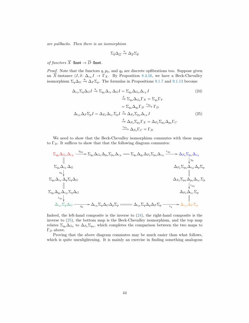
are pullbacks. Then there is an isomorphism

Σq∆G

�−→ ∆FΣp

of functors X–Inst→ D–Inst.

Proof. Note that the functors q, p0, and q0 are discrete opfibrations too. Suppose givenan X-instance (I, δ : ∆iX I → ΓX . By Proposition 8.4.16, we have a Beck-Chevalleyisomorphism Σq∆G

�−→ ∆FΣp. The formulas in Propositions 9.1.7 and 9.1.13 become

∆iDΣq∆GI�−→ Σq0∆iY ∆GI = Σq0∆G0∆iX I (24)

δ−→ Σq0∆G0ΓX = Σq0ΓY

= Σq0∆q0ΓDεq0−−→ ΓD

∆iD∆FΣpI = ∆F0∆iCΣpI�−→ ∆F0Σp0∆iX I (25)δ−→ ∆F0Σp0ΓX = ∆F0Σp0∆p0ΓCεp0−−→ ∆F0ΓC = ΓD

We need to show that the Beck-Chevalley isomorphism commutes with these mapsto ΓD. It suffices to show that that the following diagram commutes:

Σq0∆G0∆iX

ηp0 // Σq0∆G0∆p0Σp0∆iX Σq0∆q0∆F0Σp0∆iX

εq0 // ∆F0Σp0∆iX

ηp��

Σq0∆iY ∆G

ηq��

∆F0Σp0∆iX∆pΣp

Σq0∆iY ∆qΣq∆G ∆F0Σp0∆p0∆iCΣpεp0��

Σq0∆q0∆iDΣq∆G

εq0 ��

∆F0∆iCΣp

∆iDΣq∆G ηp// ∆iDΣq∆G∆pΣp ∆iDΣq∆q∆FΣp εq

// ∆iD∆FΣp

Indeed, the left-hand composite is the inverse to (24), the right-hand composite is theinverse to (25), the bottom map is the Beck-Chevalley isomorphism, and the top maprelates Σq0∆G0 to ∆F0Σp0 , which completes the comparison between the two maps toΓD above.

Proving that the above diagram commutes may be much easier than what follows,which is quite unenlightening. It is mainly an exercise in finding something analogous

44

to a least common denominator in the square above. We include it for completeness.

∆F0 Σp0 ∆iX

ηp // ∆F0 Σp0 ∆iX∆pΣp ∆F0 Σp0 ∆p0 ∆iCΣpεp0

��

Σq0 ∆q0 ∆F0 Σp0 ∆iX

εq0

OO

ηp// Σq0 ∆q0 ∆F0 Σp0 ∆iX∆pΣp

εq0

OO

Σq0 ∆q0 ∆F0 Σp0 ∆p0 ∆iCΣpεp0��

εq0

OO

Σq0 ∆G0 ∆iX

ηp0

OO

ηp // Σq0 ∆G0 ∆iX∆pΣp

ηp0

OO

Σq0 ∆q0 ∆F0 ∆iCΣpεq0 // ∆F0 ∆iCΣp

Σq0 ∆iY ∆G

ηq��

ηp // Σq0 ∆iY ∆G∆pΣpηq��

Σq0 ∆q0 ∆iD∆FΣpεq0 // ∆iD∆FΣp

Σq0 ∆q0 ∆iDΣq∆G

εq0��

ηp // Σq0 ∆q0 ∆iDΣq∆G∆pΣpεq0��

Σq0 ∆q0 ∆iDΣq∆q∆FΣp

εq

OO

εq0��

∆iDΣq∆G

ηp // ∆iDΣq∆G∆pΣp ∆iDΣq∆q∆FΣp

εq

CC

Every square in the above diagram clearly commutes, completing the proof.�

Proposition 9.2.5 (Typed distributivity). Suppose given the diagram of typed signa-tures

Set C0ΓCoo iC //

u0

��

yC

u

��B0

ΓB

aa

iB //

iA

77Bf // A

such that u is a discrete op-fibration and the square is a pullback. Note that u = (u, u0)is Σ-ready and that f = (f, idB0) is Π-ready. Construct the typed distributivity diagram

N0iN //

e0

��

yN

g //

e

��

yM

v

��

C0iC //

u0

��

yC

u

��B0

iB // Bf // A

as follows. First form the distributivity diagram as in Proposition 8.4.18, which is thebig rectangle to the right. Now take N0 to be the pullback of either the top-left square, thebig-left rectangle, or the big outer square — all are equivalent. The functors v and e arediscrete opfibrations. Note that g = (g, idN0) is Π-ready and v = (v, u0 ◦ e0) is Σ-ready.

Then there is an isomorphism

ΣvΠg∆e�−→ ΠfΣu

of functors C–Inst→ A–Inst.

Proof. By Proposition 8.4.18 we have a distributivity isomorphism

ΣvΠg∆e�−→ ΠfΣu (26)

45

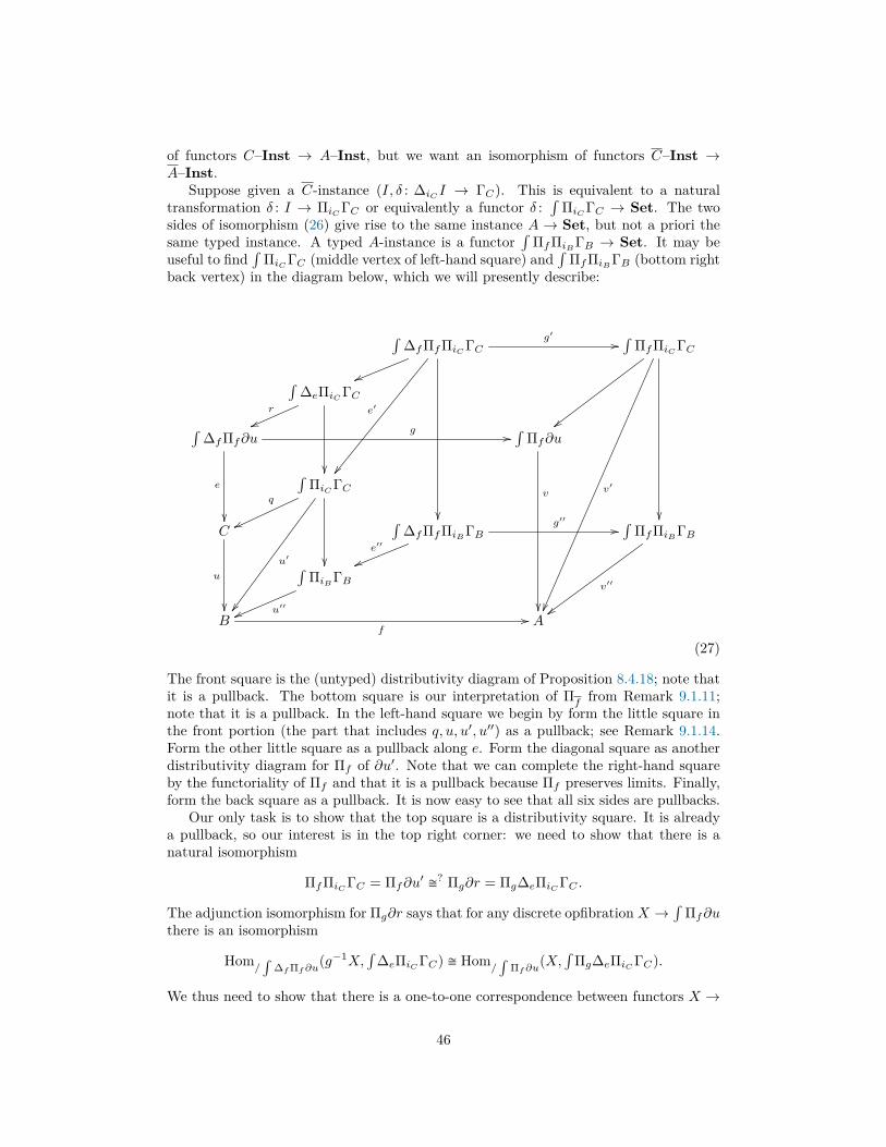
of functors C–Inst → A–Inst, but we want an isomorphism of functors C–Inst →A–Inst.

Suppose given a C-instance (I, δ : ∆iC I → ΓC). This is equivalent to a naturaltransformation δ : I → ΠiCΓC or equivalently a functor δ :

∫ΠiCΓC → Set. The two

sides of isomorphism (26) give rise to the same instance A → Set, but not a priori thesame typed instance. A typed A-instance is a functor

∫ΠfΠiBΓB → Set. It may be

useful to find∫

ΠiCΓC (middle vertex of left-hand square) and∫

ΠfΠiBΓB (bottom rightback vertex) in the diagram below, which we will presently describe:

∫∆fΠfΠiCΓC

g′ //

e′

��

vv

��

∫ΠfΠiCΓC

v′

��

{{

��

∫∆eΠiCΓC

��

r

vv∫∆fΠf∂u

g //

e

��

∫Πf∂u

v

��

∫ΠiCΓC

q

vv

u′

��

��

C

u

��

∫∆fΠfΠiBΓB

g′′ //e′′

vv

∫ΠfΠiBΓB

v′′

{{

∫ΠiBΓB

u′′vvB

f// A

(27)

The front square is the (untyped) distributivity diagram of Proposition 8.4.18; note thatit is a pullback. The bottom square is our interpretation of Πf from Remark 9.1.11;note that it is a pullback. In the left-hand square we begin by form the little square inthe front portion (the part that includes q, u, u′, u′′) as a pullback; see Remark 9.1.14.Form the other little square as a pullback along e. Form the diagonal square as anotherdistributivity diagram for Πf of ∂u′. Note that we can complete the right-hand squareby the functoriality of Πf and that it is a pullback because Πf preserves limits. Finally,form the back square as a pullback. It is now easy to see that all six sides are pullbacks.

Our only task is to show that the top square is a distributivity square. It is alreadya pullback, so our interest is in the top right corner: we need to show that there is anatural isomorphism

ΠfΠiCΓC = Πf∂u′ �? Πg∂r = Πg∆eΠiCΓC .

The adjunction isomorphism for Πg∂r says that for any discrete opfibration X →∫

Πf∂uthere is an isomorphism

Hom/∫

∆fΠf∂u(g−1X,

∫∆eΠiCΓC) � Hom

/∫

Πf∂u(X,

∫Πg∆eΠiCΓC).

We thus need to show that there is a one-to-one correspondence between functors X →

46

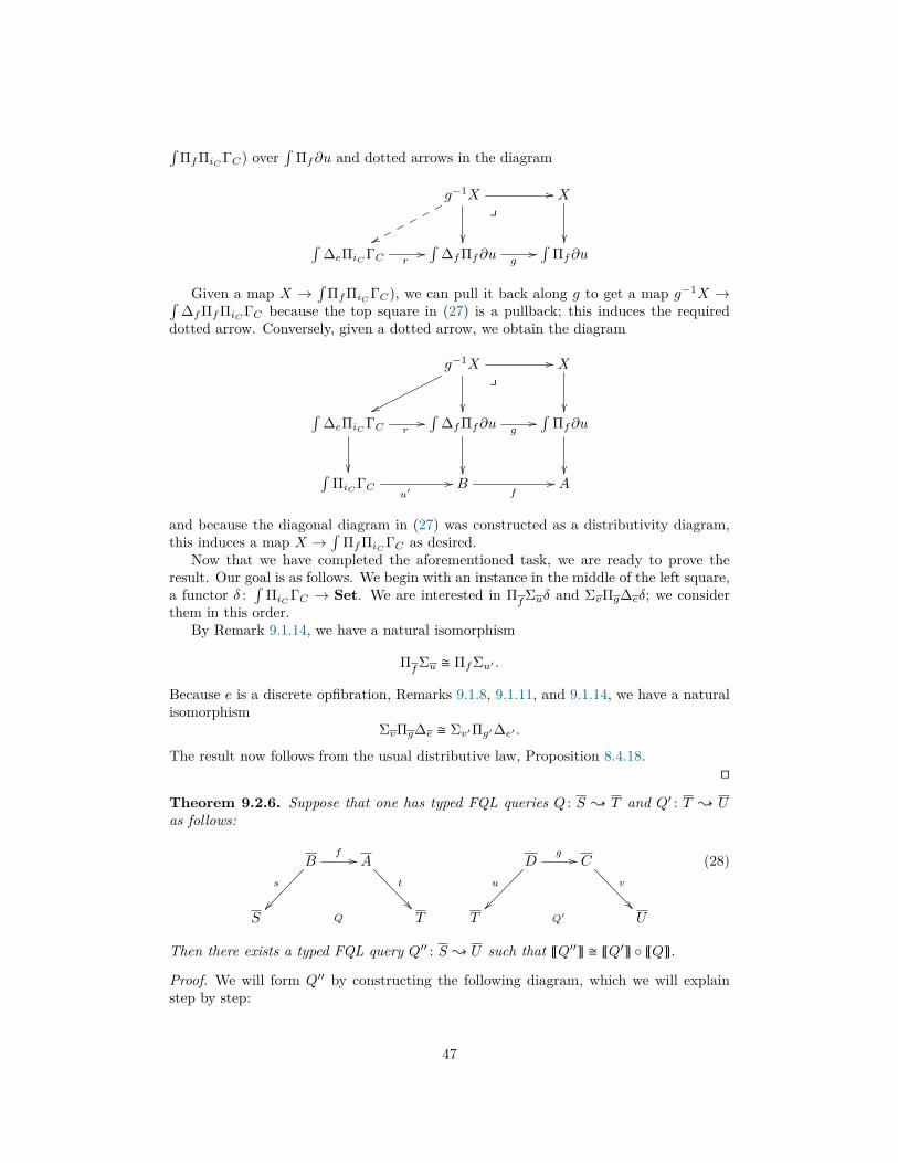
∫ΠfΠiCΓC) over

∫Πf∂u and dotted arrows in the diagram

g−1Xy

//

��ww

X

��∫∆eΠiCΓC r

//∫

∆fΠf∂u g//∫

Πf∂u

Given a map X →∫

ΠfΠiCΓC), we can pull it back along g to get a map g−1X →∫∆fΠfΠiCΓC because the top square in (27) is a pullback; this induces the required

dotted arrow. Conversely, given a dotted arrow, we obtain the diagram

g−1Xy

//

��ww

X

��∫∆eΠiCΓC r

//

��

∫∆fΠf∂u g

//

��

∫Πf∂u

��∫ΠiCΓC

u′// B

f// A

and because the diagonal diagram in (27) was constructed as a distributivity diagram,this induces a map X →

∫ΠfΠiCΓC as desired.

Now that we have completed the aforementioned task, we are ready to prove theresult. Our goal is as follows. We begin with an instance in the middle of the left square,a functor δ :

∫ΠiCΓC → Set. We are interested in ΠfΣuδ and ΣvΠg∆eδ; we consider

them in this order.By Remark 9.1.14, we have a natural isomorphism

ΠfΣu � ΠfΣu′ .

Because e is a discrete opfibration, Remarks 9.1.8, 9.1.11, and 9.1.14, we have a naturalisomorphism

ΣvΠg∆e � Σv′Πg′∆e′ .

The result now follows from the usual distributive law, Proposition 8.4.18.�

Theorem 9.2.6. Suppose that one has typed FQL queries Q : S { T and Q′ : T { Uas follows:

Bf //

s

��

A

t

��

Dg //

u

��

C

v

��S Q T T Q′ U

(28)

Then there exists a typed FQL query Q′′ : S { U such that ~Q′′� � ~Q′� ◦ ~Q�.

Proof. We will form Q′′ by constructing the following diagram, which we will explainstep by step:

47

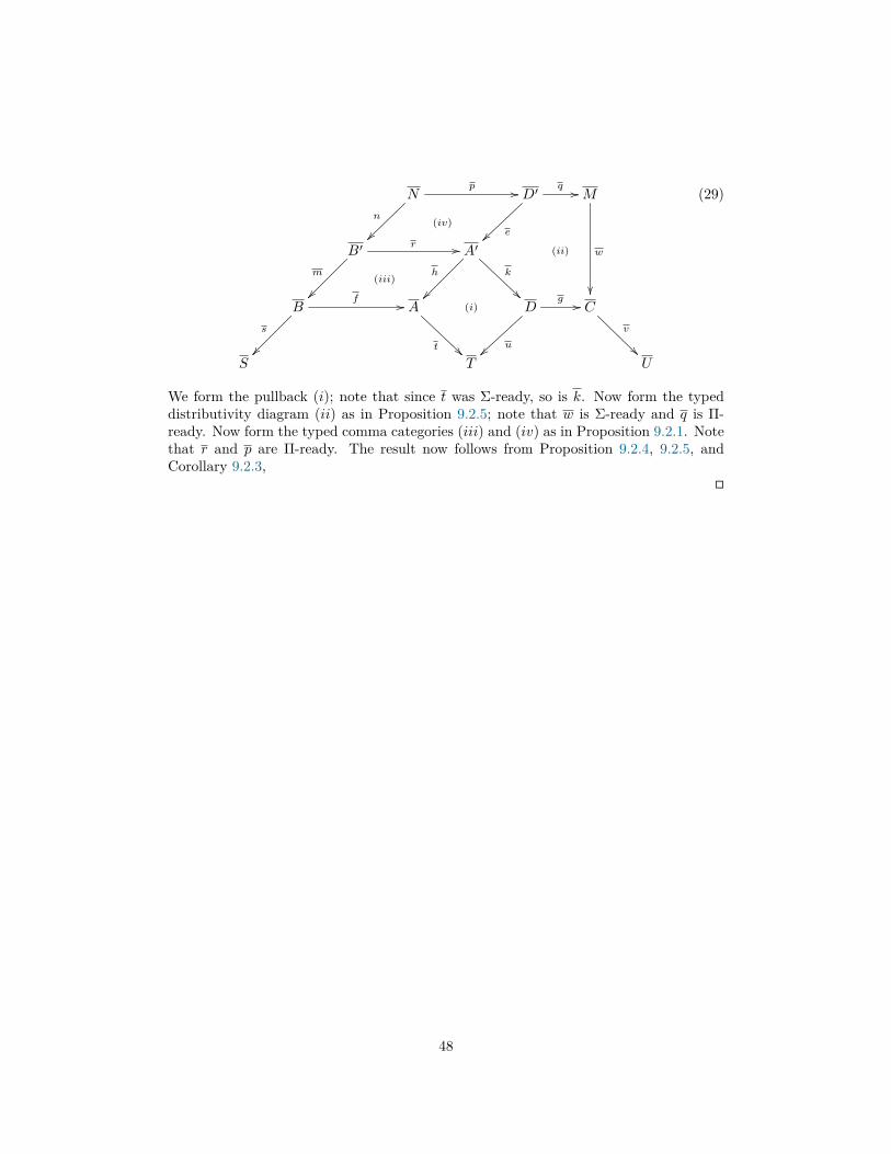
Np //

n

��(iv)

D′q //

e~~(ii)

M

w

��

B′r //

m

��(iii)

A′

k

h

��(i)B

s

��

f // A

t ��

D

u~~

g // C

v

��S T U

(29)

We form the pullback (i); note that since t was Σ-ready, so is k. Now form the typeddistributivity diagram (ii) as in Proposition 9.2.5; note that w is Σ-ready and q is Π-ready. Now form the typed comma categories (iii) and (iv) as in Proposition 9.2.1. Notethat r and p are Π-ready. The result now follows from Proposition 9.2.4, 9.2.5, andCorollary 9.2.3,

�

48