Relational Query Optimization

CS186R & G Chapters 12/15

Review

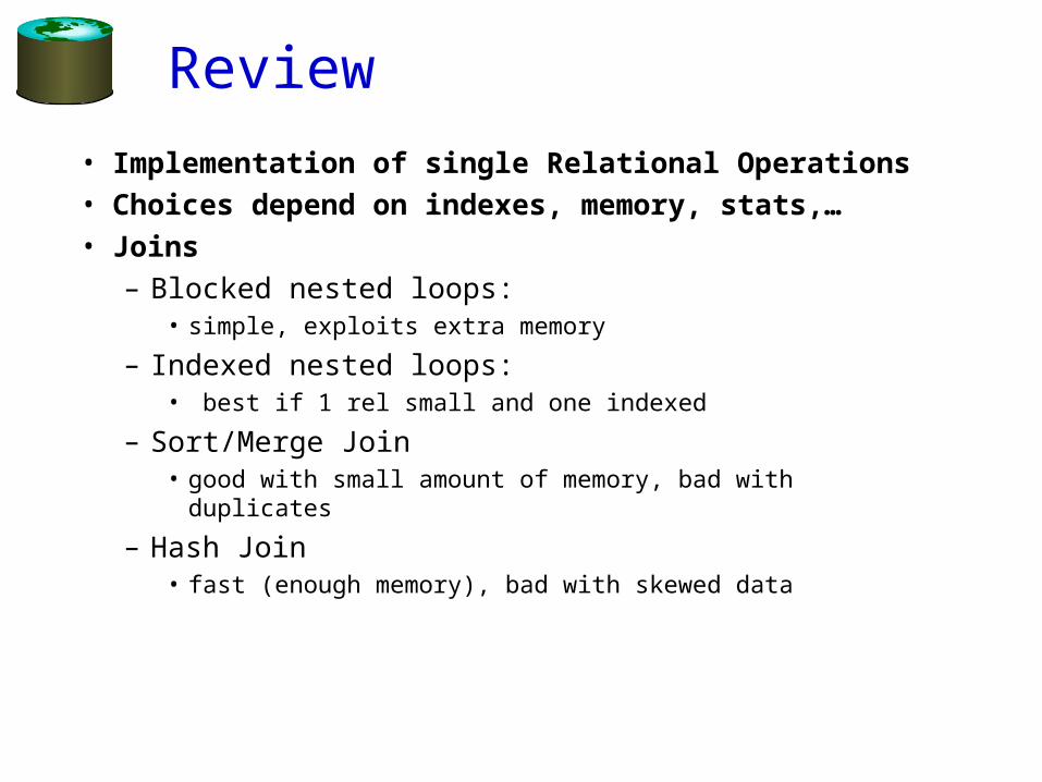
• Implementation of single Relational Operations• Choices depend on indexes, memory, stats,…• Joins

– Blocked nested loops:• simple, exploits extra memory

– Indexed nested loops:• best if 1 rel small and one indexed

– Sort/Merge Join• good with small amount of memory, bad with duplicates

– Hash Join• fast (enough memory), bad with skewed data

Query Optimization Overview

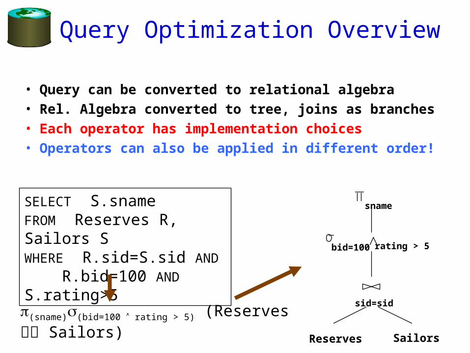
SELECT S.snameFROM Reserves R, Sailors SWHERE R.sid=S.sid AND R.bid=100 AND S.rating>5

Reserves Sailors

sid=sid

bid=100 rating > 5

sname

• Query can be converted to relational algebra• Rel. Algebra converted to tree, joins as branches• Each operator has implementation choices• Operators can also be applied in different order!

(sname)(bid=100 rating > 5) (Reserves Sailors)

Query Optimization Overview (cont.)

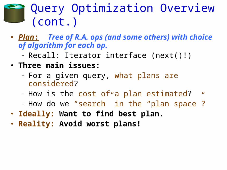
• Plan: Tree of R.A. ops (and some others) with choice of algorithm for each op.– Recall: Iterator interface (next()!)

• Three main issues:– For a given query, what plans are considered?– How is the cost of a plan estimated?– How do we “search” in the “plan space”?

• Ideally: Want to find best plan. • Reality: Avoid worst plans!

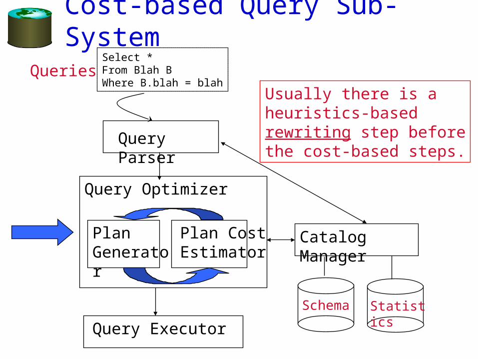
Cost-based Query Sub-System

Query Parser

Query Optimizer

Plan Generator

Plan Cost Estimator

Query Executor

Catalog Manager

Usually there is aheuristics-basedrewriting step beforethe cost-based steps.

Schema

Statistics

Select *From Blah BWhere B.blah = blah

Queries

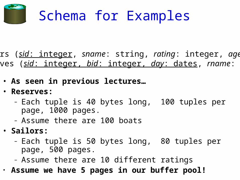
Schema for Examples

• As seen in previous lectures…• Reserves:

– Each tuple is 40 bytes long, 100 tuples per page, 1000 pages.

– Assume there are 100 boats• Sailors:

– Each tuple is 50 bytes long, 80 tuples per page, 500 pages.

– Assume there are 10 different ratings • Assume we have 5 pages in our buffer pool!

Sailors (sid: integer, sname: string, rating: integer, age: real)Reserves (sid: integer, bid: integer, day: dates, rname: string)

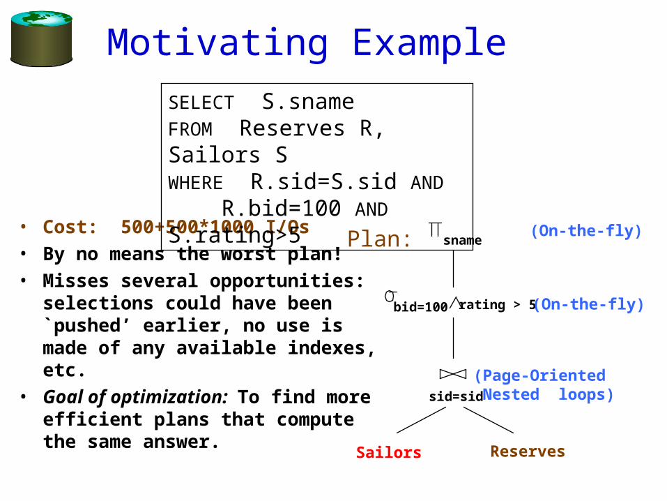
Motivating Example

• Cost: 500+500*1000 I/Os• By no means the worst plan! • Misses several opportunities:

selections could have been `pushed’ earlier, no use is made of any available indexes, etc.

• Goal of optimization: To find more efficient plans that compute the same answer.

SELECT S.snameFROM Reserves R, Sailors SWHERE R.sid=S.sid AND R.bid=100 AND S.rating>5

Sailors Reserves

sid=sid

bid=100 rating > 5

sname

(Page-Oriented Nested loops)

(On-the-fly)

(On-the-fly)Plan:

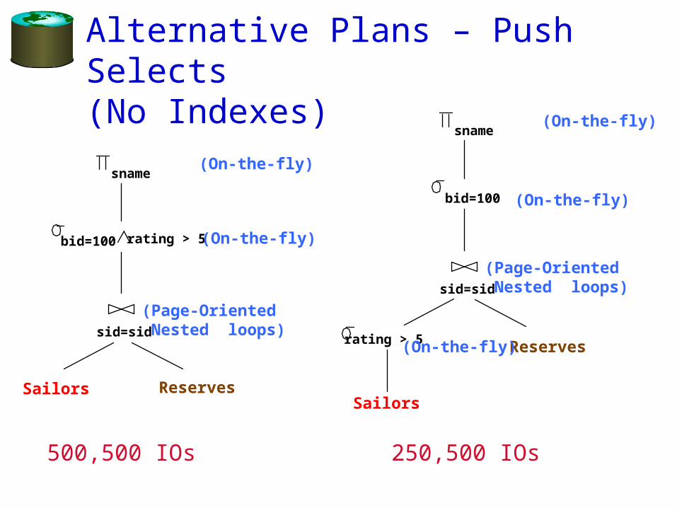
500,500 IOs

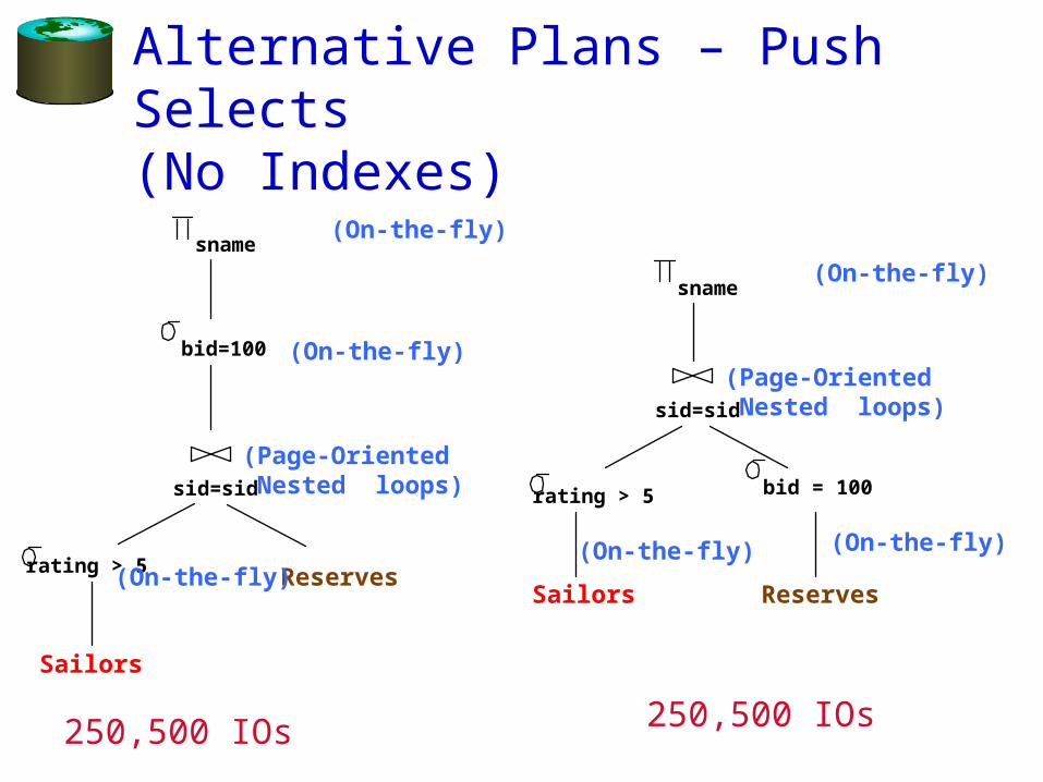
Alternative Plans – Push Selects (No Indexes)

Sailors Reserves

sid=sid

bid=100 rating > 5

sname

(Page-Oriented Nested loops)

(On-the-fly)

(On-the-fly)

Sailors

Reserves

sid=sid

rating > 5

sname

(Page-Oriented Nested loops)

(On-the-fly)

(On-the-fly)

bid=100 (On-the-fly)

250,500 IOs

Alternative Plans – Push Selects (No Indexes)

Sailors

Reserves

sid=sid

rating > 5

sname

(Page-Oriented Nested loops)

(On-the-fly)

(On-the-fly)

bid=100 (On-the-fly)

Sailors Reserves

sid=sid

bid = 100

sname

(Page-Oriented Nested loops)

(On-the-fly)

rating > 5

(On-the-fly)(On-the-fly)

250,500 IOs250,500 IOs

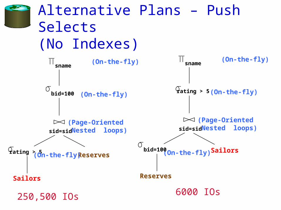
Sailors

Reserves

sid=sid

rating > 5

sname

(Page-Oriented Nested loops)

(On-the-fly)

(On-the-fly)

bid=100 (On-the-fly)

6000 IOs

Sailors

Reserves

sid=sid

rating > 5

sname

(Page-Oriented Nested loops)

(On-the-fly)

(On-the-fly)

bid=100

(On-the-fly)

250,500 IOs

Alternative Plans – Push Selects (No Indexes)

SailorsReserves

sid=sid

rating > 5

sname

(Page-Oriented Nested loops)

(On-the-fly)

bid=100

(Scan &Write totemp T2)(On-the-fly)

6000 IOs

Sailors

Reserves

sid=sid

rating > 5

sname

(Page-Oriented Nested loops)

(On-the-fly)

(On-the-fly)

bid=100

(On-the-fly)

Alternative Plans – Push Selects (No Indexes)

4250 IOs1000 + 500+ 250 + (10 * 250)

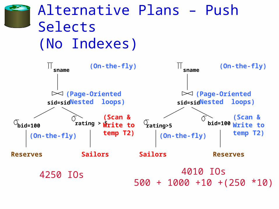
ReservesSailors

sid=sid

bid=100

sname

(Page-Oriented Nested loops)

(On-the-fly)

rating>5

(Scan &Write totemp T2)(On-the-fly)

Alternative Plans – Push Selects (No Indexes)

4010 IOs500 + 1000 +10 +(250 *10)

SailorsReserves

sid=sid

rating > 5

sname

(Page-Oriented Nested loops)

(On-the-fly)

bid=100

(Scan &Write totemp T2)(On-the-fly)

4250 IOs

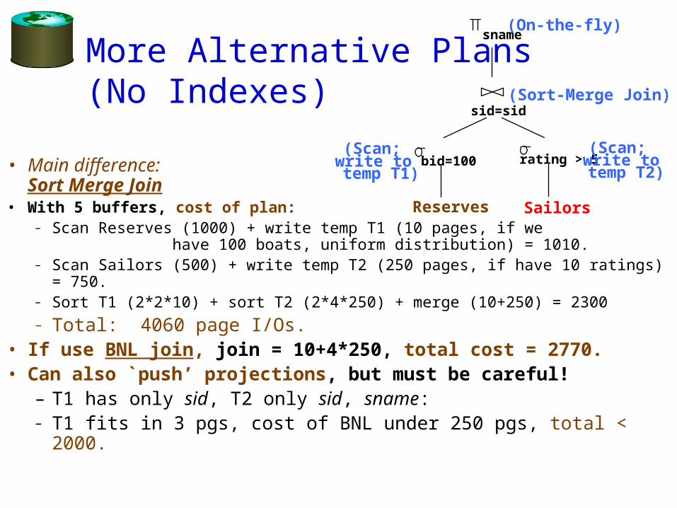
More Alternative Plans (No Indexes)

• Main difference: Sort Merge Join

• With 5 buffers, cost of plan:– Scan Reserves (1000) + write temp T1 (10 pages, if we

have 100 boats, uniform distribution) = 1010.– Scan Sailors (500) + write temp T2 (250 pages, if have 10 ratings) =

750.– Sort T1 (2*2*10) + sort T2 (2*4*250) + merge (10+250) = 2300– Total: 4060 page I/Os.

• If use BNL join, join = 10+4*250, total cost = 2770.• Can also `push’ projections, but must be careful!

– T1 has only sid, T2 only sid, sname:– T1 fits in 3 pgs, cost of BNL under 250 pgs, total < 2000.

Reserves Sailors

sid=sid

bid=100

sname(On-the-fly)

rating > 5(Scan;write to temp T1)

(Scan;write totemp T2)

(Sort-Merge Join)

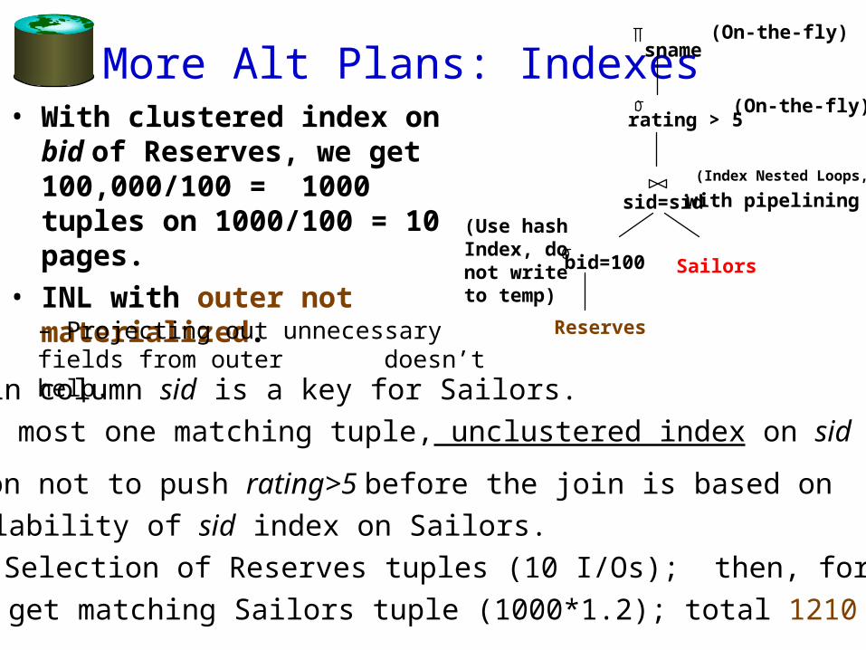
More Alt Plans: Indexes• With clustered index on

bid of Reserves, we get 100,000/100 = 1000 tuples on 1000/100 = 10 pages.

• INL with outer not materialized.

Decision not to push rating>5 before the join is based on availability of sid index on Sailors. Cost: Selection of Reserves tuples (10 I/Os); then, for each, must get matching Sailors tuple (1000*1.2); total 1210 I/Os.

Join column sid is a key for Sailors.–At most one matching tuple, unclustered index on sid OK.

– Projecting out unnecessary fields from outer doesn’t help.

(On-the-fly)

(Use hashIndex, donot writeto temp)

Reserves

Sailors

sid=sid

bid=100

sname

rating > 5

(Index Nested Loops,

with pipelining )

(On-the-fly)

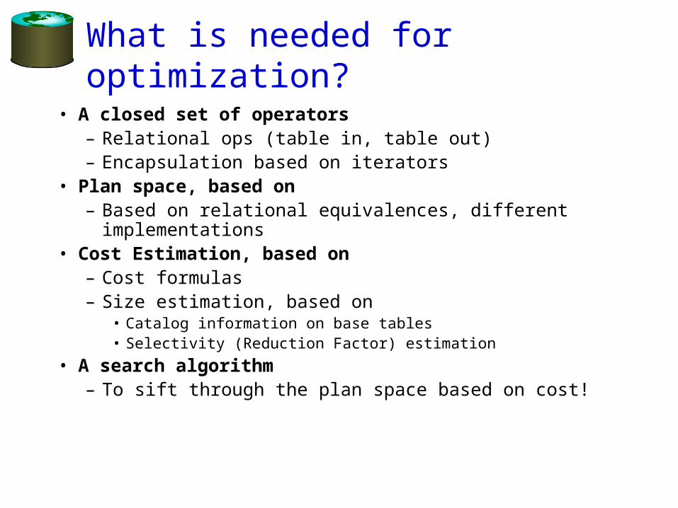
What is needed for optimization?

• A closed set of operators – Relational ops (table in, table out)– Encapsulation based on iterators

• Plan space, based on– Based on relational equivalences, different

implementations• Cost Estimation, based on

– Cost formulas– Size estimation, based on

• Catalog information on base tables• Selectivity (Reduction Factor) estimation

• A search algorithm– To sift through the plan space based on cost!

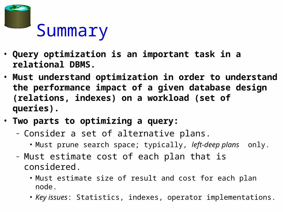
Summary• Query optimization is an important task in a

relational DBMS.• Must understand optimization in order to

understand the performance impact of a given database design (relations, indexes) on a workload (set of queries).

• Two parts to optimizing a query:– Consider a set of alternative plans.

• Must prune search space; typically, left-deep plans only.

– Must estimate cost of each plan that is considered.• Must estimate size of result and cost for each plan node.• Key issues: Statistics, indexes, operator implementations.

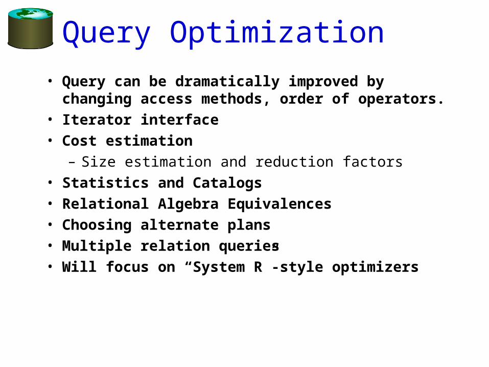
Query Optimization• Query can be dramatically improved by

changing access methods, order of operators.• Iterator interface• Cost estimation

– Size estimation and reduction factors• Statistics and Catalogs• Relational Algebra Equivalences• Choosing alternate plans• Multiple relation queries• Will focus on “System R”-style optimizers

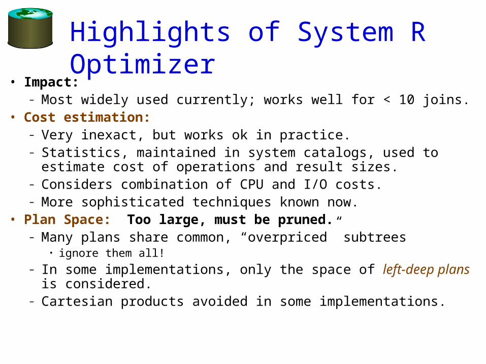
Highlights of System R Optimizer

• Impact:– Most widely used currently; works well for < 10 joins.

• Cost estimation:– Very inexact, but works ok in practice.– Statistics, maintained in system catalogs, used to estimate

cost of operations and result sizes.– Considers combination of CPU and I/O costs.– More sophisticated techniques known now.

• Plan Space: Too large, must be pruned.– Many plans share common, “overpriced” subtrees

• ignore them all!– In some implementations, only the space of left-deep plans is

considered.– Cartesian products avoided in some implementations.

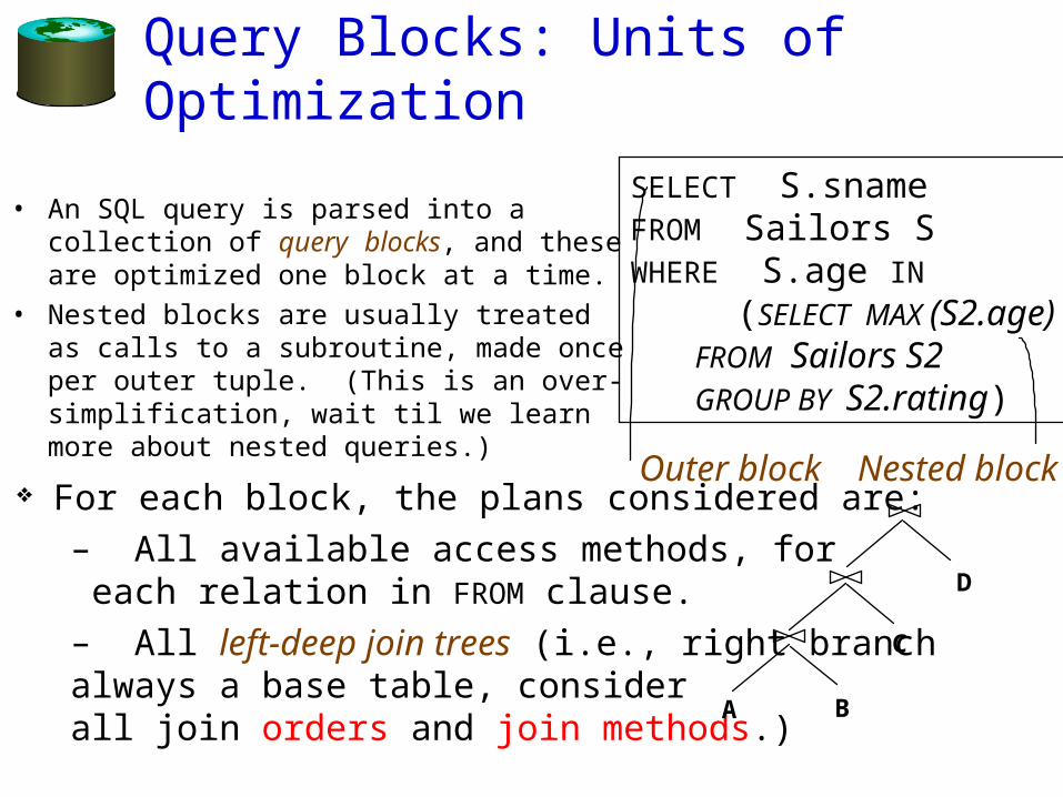
Query Blocks: Units of Optimization

• An SQL query is parsed into a collection of query blocks, and these are optimized one block at a time.

• Nested blocks are usually treated as calls to a subroutine, made once per outer tuple. (This is an over-simplification, wait til we learn more about nested queries.)

SELECT S.snameFROM Sailors SWHERE S.age IN (SELECT MAX (S2.age) FROM Sailors S2 GROUP BY S2.rating)

Nested blockOuter block For each block, the plans considered are:

– All available access methods, for each relation in FROM clause.– All left-deep join trees (i.e., right branchalways a base table, considerall join orders and join methods.)

BA

C

D

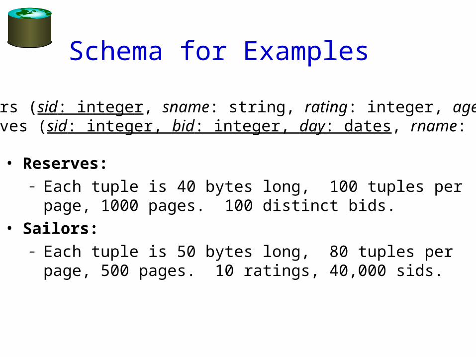
Schema for Examples

• Reserves:– Each tuple is 40 bytes long, 100 tuples per page,

1000 pages. 100 distinct bids.• Sailors:

– Each tuple is 50 bytes long, 80 tuples per page, 500 pages. 10 ratings, 40,000 sids.

Sailors (sid: integer, sname: string, rating: integer, age: real)Reserves (sid: integer, bid: integer, day: dates, rname: string)

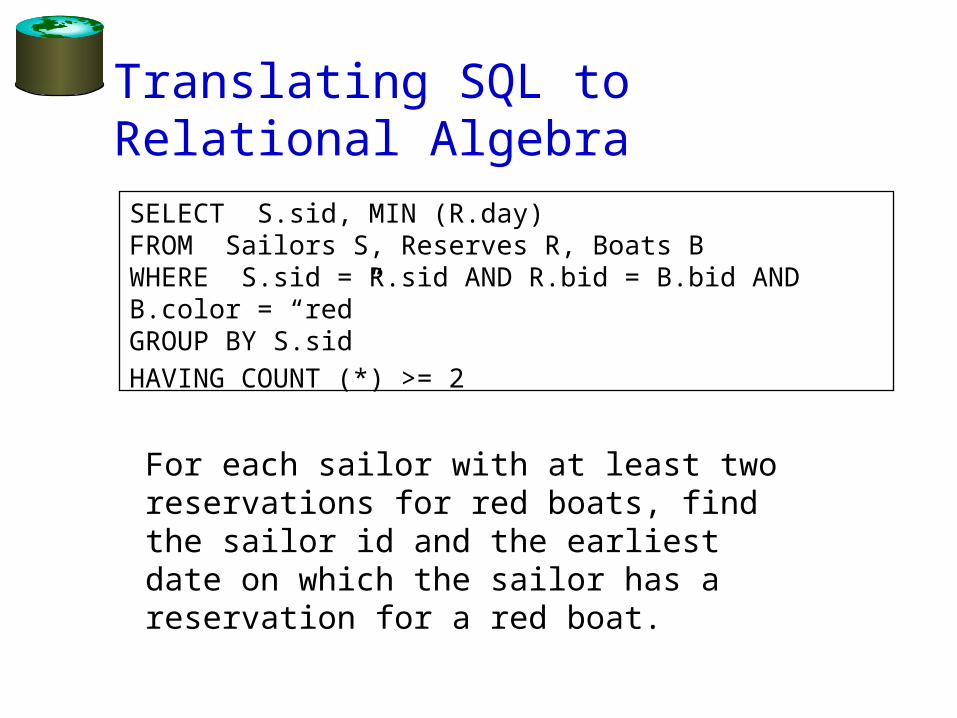
Translating SQL to Relational AlgebraSELECT S.sid, MIN (R.day)FROM Sailors S, Reserves R, Boats BWHERE S.sid = R.sid AND R.bid = B.bid AND B.color = “red”GROUP BY S.sidHAVING COUNT (*) >= 2

For each sailor with at least two reservations for red boats, find the sailor id and the earliest date on which the sailor has a reservation for a red boat.

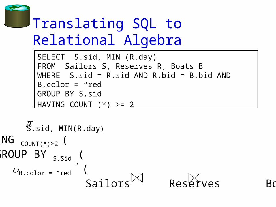
S.sid, MIN(R.day)

(HAVING COUNT(*)>2 ( GROUP BY S.Sid (B.color = “red” ( Sailors Reserves Boats))))

Translating SQL to Relational AlgebraSELECT S.sid, MIN (R.day)FROM Sailors S, Reserves R, Boats BWHERE S.sid = R.sid AND R.bid = B.bid AND B.color = “red”GROUP BY S.sidHAVING COUNT (*) >= 2

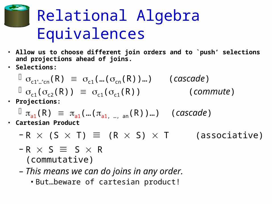
• Allow us to choose different join orders and to `push’ selections and projections ahead of joins.

• Selections:

c1…cn(R) c1(…(cn(R))…) (cascade) c1(c2(R)) c1(c1(R)) (commute)

• Projections:

a1(R) a1(…(a1, …, an(R))…) (cascade)• Cartesian Product

– R (S T) (R S) T (associative)

– R S S R (commutative)– This means we can do joins in any order.

• But…beware of cartesian product!

Relational Algebra Equivalences

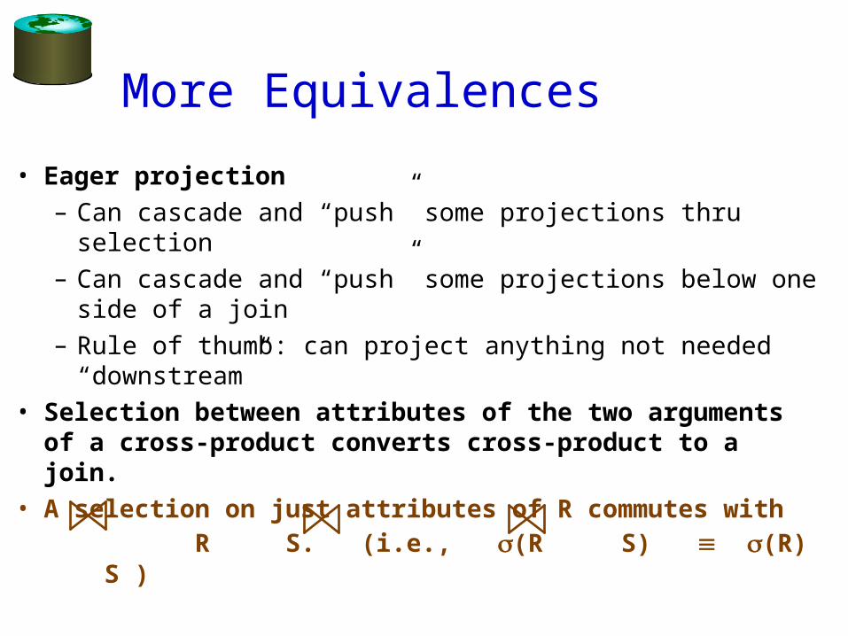
More Equivalences

• Eager projection– Can cascade and “push” some projections thru

selection– Can cascade and “push” some projections below one

side of a join– Rule of thumb: can project anything not needed

“downstream”• Selection between attributes of the two arguments

of a cross-product converts cross-product to a join.• A selection on just attributes of R commutes with

R S. (i.e., (R S) (R) S )

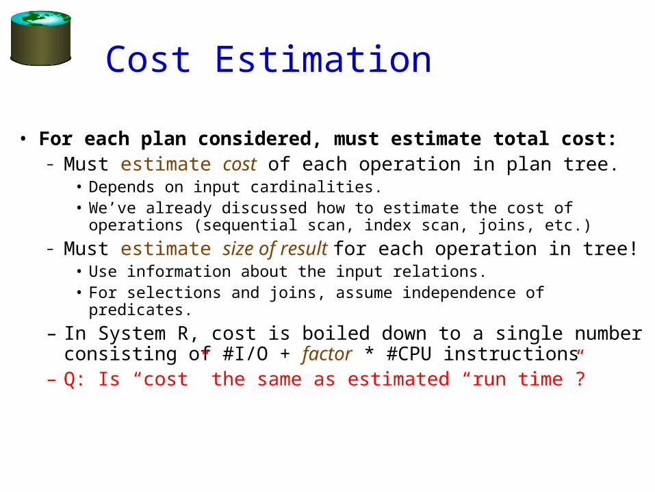
Cost Estimation

• For each plan considered, must estimate total cost:– Must estimate cost of each operation in plan tree.

• Depends on input cardinalities.• We’ve already discussed how to estimate the cost of

operations (sequential scan, index scan, joins, etc.)– Must estimate size of result for each operation in

tree!• Use information about the input relations.• For selections and joins, assume independence of

predicates.

– In System R, cost is boiled down to a single number consisting of #I/O + factor * #CPU instructions

– Q: Is “cost” the same as estimated “run time”?

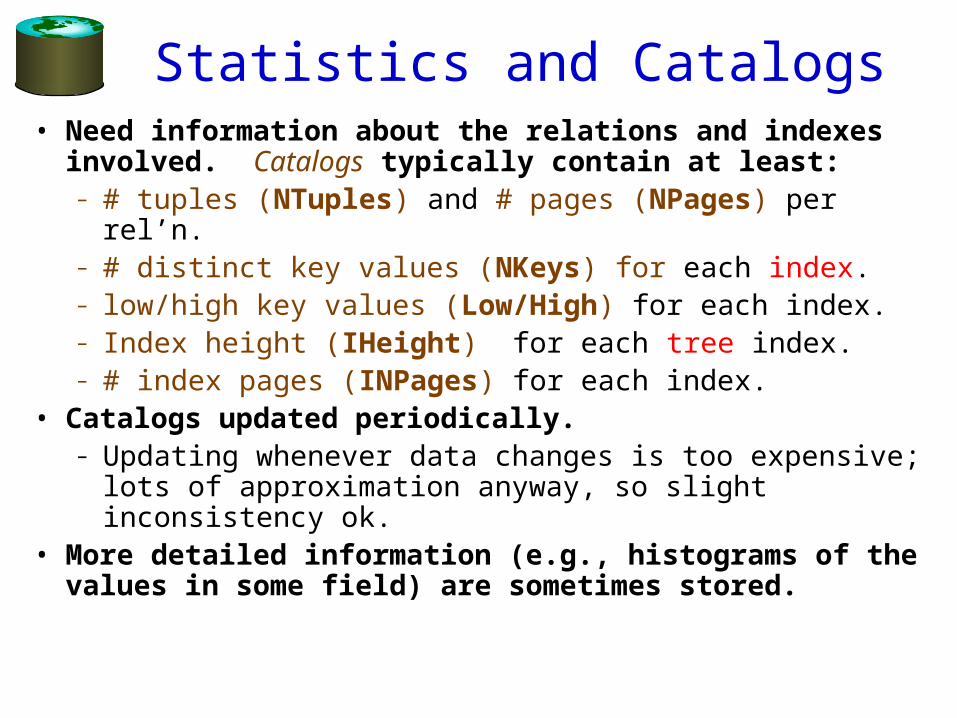
Statistics and Catalogs• Need information about the relations and indexes

involved. Catalogs typically contain at least:– # tuples (NTuples) and # pages (NPages) per rel’n.– # distinct key values (NKeys) for each index.– low/high key values (Low/High) for each index.– Index height (IHeight) for each tree index.– # index pages (INPages) for each index.

• Catalogs updated periodically.– Updating whenever data changes is too expensive; lots

of approximation anyway, so slight inconsistency ok.• More detailed information (e.g., histograms of the

values in some field) are sometimes stored.

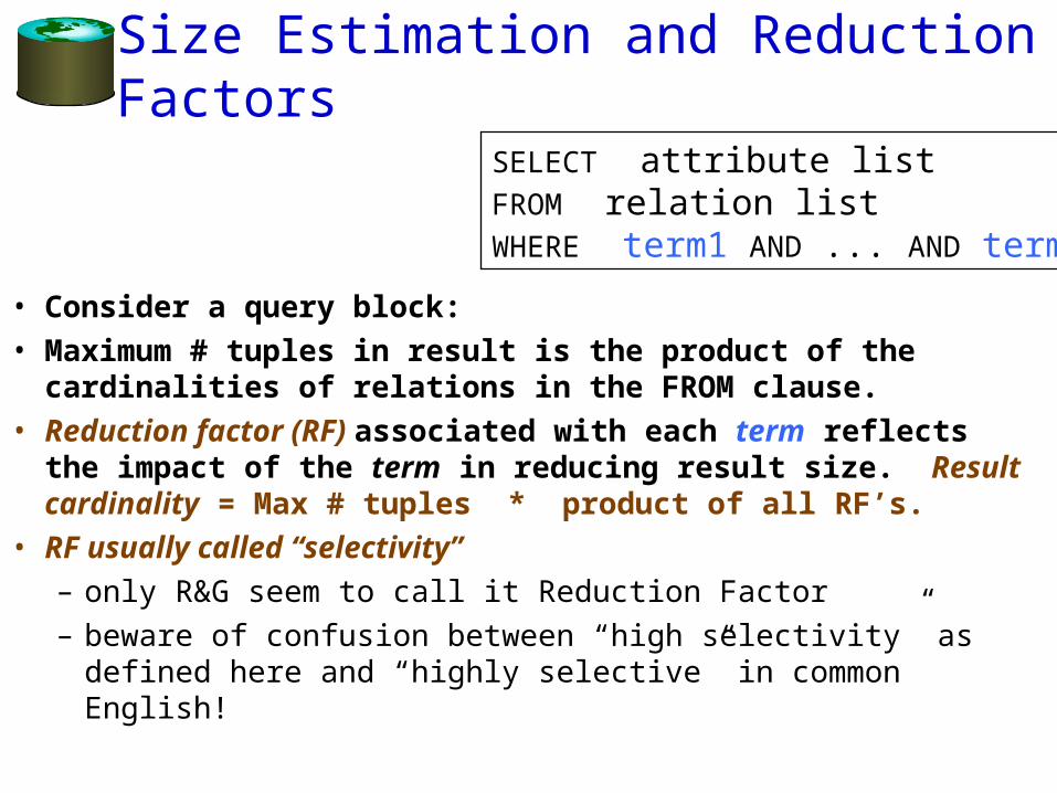
Size Estimation and Reduction Factors

• Consider a query block:• Maximum # tuples in result is the product of the

cardinalities of relations in the FROM clause.• Reduction factor (RF) associated with each term

reflects the impact of the term in reducing result size. Result cardinality = Max # tuples * product of all RF’s.

• RF usually called “selectivity”– only R&G seem to call it Reduction Factor– beware of confusion between “high selectivity” as defined

here and “highly selective” in common English!

SELECT attribute listFROM relation listWHERE term1 AND ... AND termk

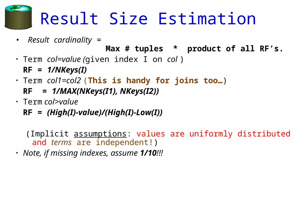
Result Size Estimation• Result cardinality = Max

# tuples * product of all RF’s.• Term col=value (given index I on col )

RF = 1/NKeys(I) • Term col1=col2 (This is handy for joins too…)

RF = 1/MAX(NKeys(I1), NKeys(I2))• Term col>value

RF = (High(I)-value)/(High(I)-Low(I))

(Implicit assumptions: values are uniformly distributed and terms are independent!)

• Note, if missing indexes, assume 1/10!!!

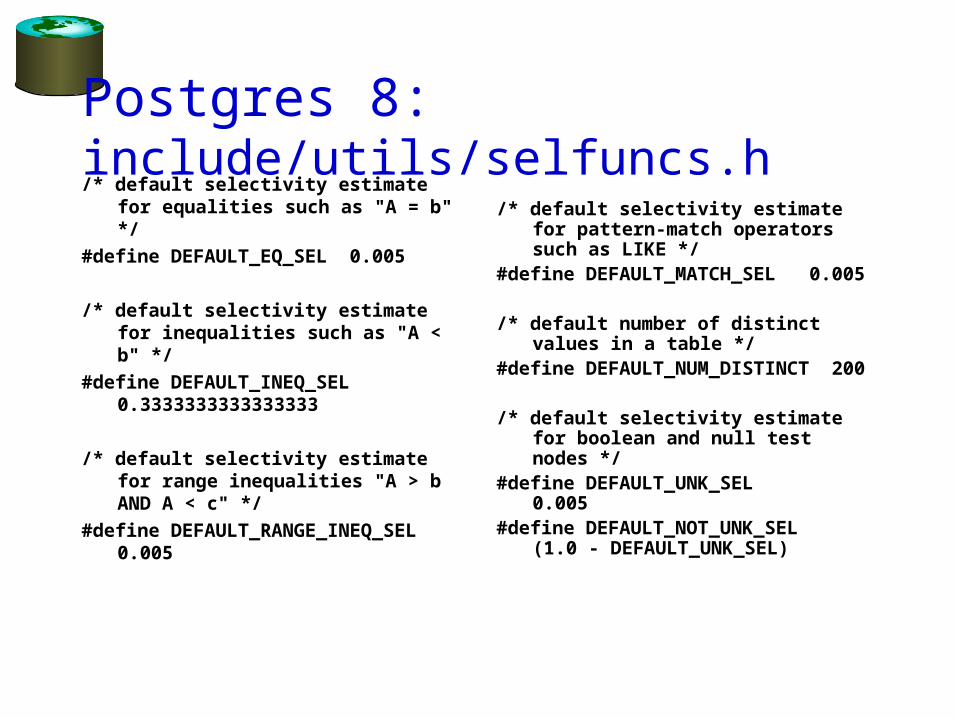
Postgres 8: include/utils/selfuncs.h/* default selectivity estimate

for equalities such as "A = b" */

#define DEFAULT_EQ_SEL 0.005

/* default selectivity estimate for inequalities such as "A < b" */

#define DEFAULT_INEQ_SEL 0.3333333333333333

/* default selectivity estimate for range inequalities "A > b AND A < c" */

#define DEFAULT_RANGE_INEQ_SEL 0.005

/* default selectivity estimate for pattern-match operators such as LIKE */

#define DEFAULT_MATCH_SEL 0.005

/* default number of distinct values in a table */

#define DEFAULT_NUM_DISTINCT 200

/* default selectivity estimate for boolean and null test nodes */

#define DEFAULT_UNK_SEL 0.005

#define DEFAULT_NOT_UNK_SEL (1.0 - DEFAULT_UNK_SEL)

Look what’s in Postgres 7.3!

/* * * THIS IS A HACK TO GET V4 OUT THE DOOR. * -- JMH 7/9/92 */s1 = (Selectivity) 0.3333333;

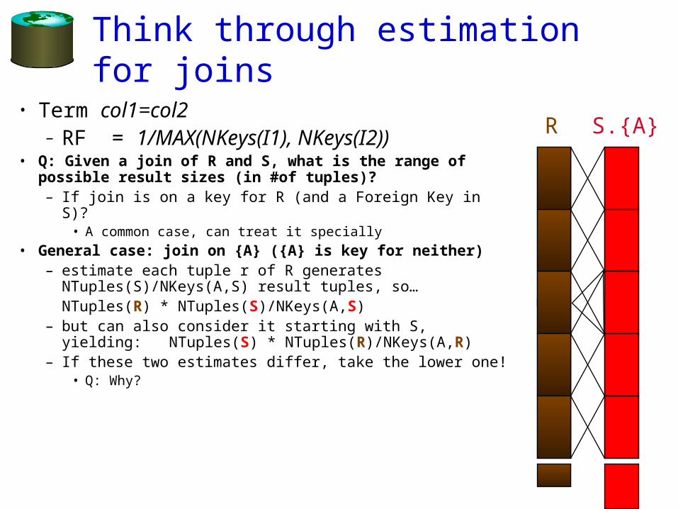
Think through estimation for joins

• Term col1=col2 – RF = 1/MAX(NKeys(I1), NKeys(I2))

• Q: Given a join of R and S, what is the range of possible result sizes (in #of tuples)?– If join is on a key for R (and a Foreign Key in S)?

• A common case, can treat it specially • General case: join on {A} ({A} is key for neither)

– estimate each tuple r of R generates NTuples(S)/NKeys(A,S) result tuples, so…

NTuples(R) * NTuples(S)/NKeys(A,S)– but can also consider it starting with S, yielding:

NTuples(S) * NTuples(R)/NKeys(A,R)– If these two estimates differ, take the lower one!

• Q: Why?

r

S.{A}R

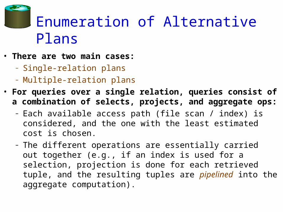
Enumeration of Alternative Plans

• There are two main cases:– Single-relation plans– Multiple-relation plans

• For queries over a single relation, queries consist of a combination of selects, projects, and aggregate ops:– Each available access path (file scan / index) is

considered, and the one with the least estimated cost is chosen.

– The different operations are essentially carried out together (e.g., if an index is used for a selection, projection is done for each retrieved tuple, and the resulting tuples are pipelined into the aggregate computation).

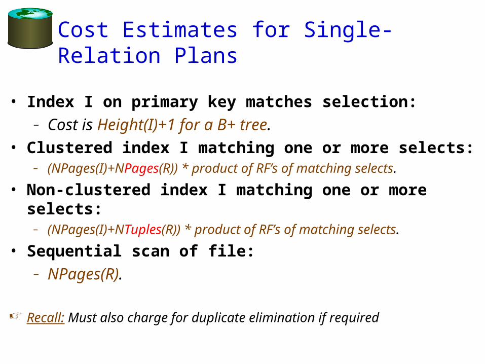
Cost Estimates for Single-Relation Plans

• Index I on primary key matches selection:– Cost is Height(I)+1 for a B+ tree.

• Clustered index I matching one or more selects:– (NPages(I)+NPages(R)) * product of RF’s of matching selects.

• Non-clustered index I matching one or more selects:– (NPages(I)+NTuples(R)) * product of RF’s of matching selects.

• Sequential scan of file:– NPages(R).

Recall: Must also charge for duplicate elimination if required

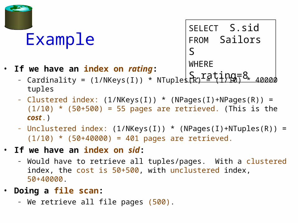
Example

• If we have an index on rating:– Cardinality = (1/NKeys(I)) * NTuples(R) = (1/10) * 40000 tuples – Clustered index: (1/NKeys(I)) * (NPages(I)+NPages(R)) = (1/10) *

(50+500) = 55 pages are retrieved. (This is the cost.)– Unclustered index: (1/NKeys(I)) * (NPages(I)+NTuples(R)) = (1/10) *

(50+40000) = 401 pages are retrieved. • If we have an index on sid:

– Would have to retrieve all tuples/pages. With a clustered index, the cost is 50+500, with unclustered index, 50+40000.

• Doing a file scan:– We retrieve all file pages (500).

SELECT S.sidFROM Sailors SWHERE S.rating=8

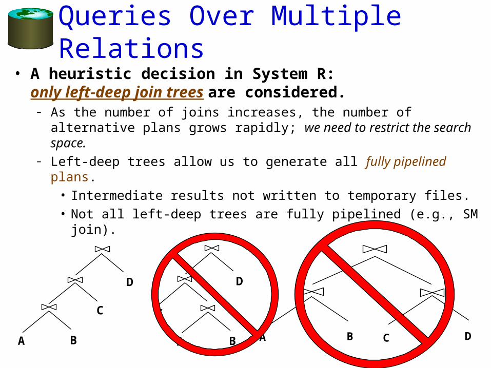
Queries Over Multiple Relations

• A heuristic decision in System R:only left-deep join trees are considered.– As the number of joins increases, the number of alternative

plans grows rapidly; we need to restrict the search space.– Left-deep trees allow us to generate all fully pipelined plans.

• Intermediate results not written to temporary files.• Not all left-deep trees are fully pipelined (e.g., SM join).

BA

C

D

BA

C

D

C DBA

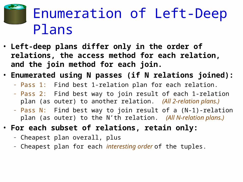
Enumeration of Left-Deep Plans

• Left-deep plans differ only in the order of relations, the access method for each relation, and the join method for each join.

• Enumerated using N passes (if N relations joined):– Pass 1: Find best 1-relation plan for each relation.– Pass 2: Find best way to join result of each 1-relation plan (as

outer) to another relation. (All 2-relation plans.) – Pass N: Find best way to join result of a (N-1)-relation plan (as

outer) to the N’th relation. (All N-relation plans.)

• For each subset of relations, retain only:– Cheapest plan overall, plus– Cheapest plan for each interesting order of the tuples.

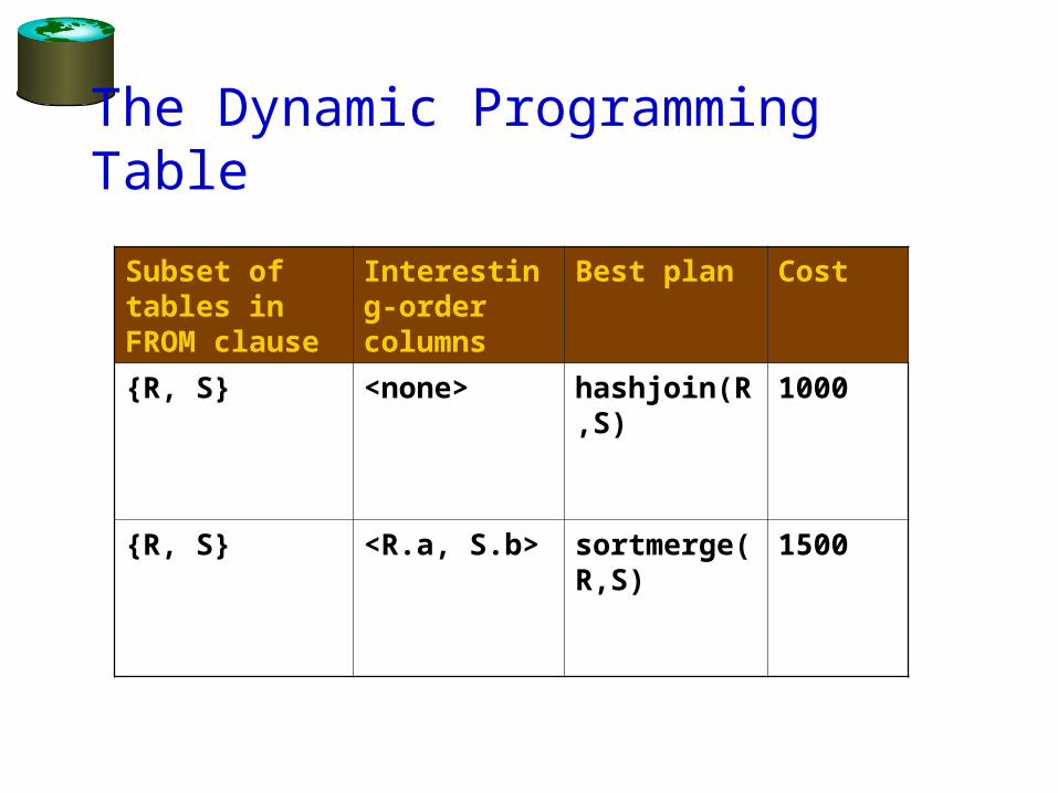
The Dynamic Programming Table

Subset of tables in FROM clause

Interesting-order columns

Best plan Cost

{R, S} <none> hashjoin(R,S)

1000

{R, S} <R.a, S.b> sortmerge(R,S)

1500

A Note on “Interesting Orders”

• An intermediate result has an “interesting order” if it is sorted by any of:

– ORDER BY attributes– GROUP BY attributes– Join attributes of yet-to-be-added

(downstream) joins

Enumeration of Plans (Contd.)

• An N-1 way plan is not combined with an additional relation unless there is a join condition between them, unless all predicates in WHERE have been used up.– i.e., avoid Cartesian products if possible.

• ORDER BY, GROUP BY, aggregates etc. handled as a final step, using either an `interestingly ordered’ plan or an additonal sort/hash operator.

• In spite of pruning plan space, this approach is still exponential in the # of tables.

• Recall that in practice, COST considered is #IOs + factor * CPU Inst

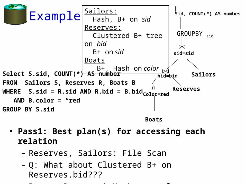
Example Sailors: Hash, B+ on sidReserves: Clustered B+ tree on bid B+ on sidBoats B+, Hash on color

Select S.sid, COUNT(*) AS numberFROM Sailors S, Reserves R, Boats BWHERE S.sid = R.sid AND R.bid = B.bid AND B.color = “red” GROUP BY S.sid

Reserves

Sailors

sid=sid

Boats

Sid, COUNT(*) AS numbes

GROUPBY sid

bid=bid

Color=red

• Pass1: Best plan(s) for accessing each relation– Reserves, Sailors: File Scan– Q: What about Clustered B+ on Reserves.bid???– Boats: B+ tree & Hash on color

Pass 1

• Best plan for accessing each relation regarded as the first relation in an execution plan– Reserves, Sailors: File Scan– Boats: B+ tree & Hash on color

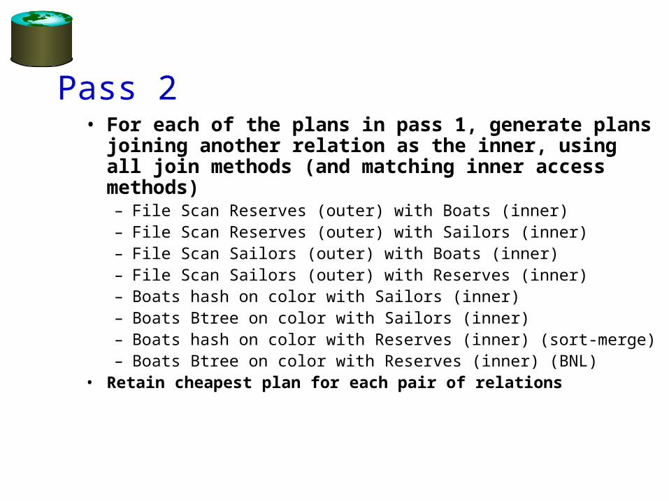
Pass 2• For each of the plans in pass 1, generate plans

joining another relation as the inner, using all join methods (and matching inner access methods)– File Scan Reserves (outer) with Boats (inner)– File Scan Reserves (outer) with Sailors (inner)– File Scan Sailors (outer) with Boats (inner)– File Scan Sailors (outer) with Reserves (inner)– Boats hash on color with Sailors (inner)– Boats Btree on color with Sailors (inner)– Boats hash on color with Reserves (inner) (sort-merge)– Boats Btree on color with Reserves (inner) (BNL)

• Retain cheapest plan for each pair of relations

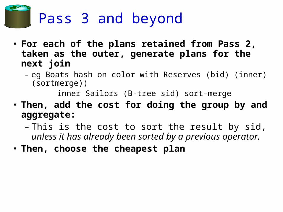
Pass 3 and beyond

• For each of the plans retained from Pass 2, taken as the outer, generate plans for the next join– eg Boats hash on color with Reserves (bid) (inner)

(sortmerge)) inner Sailors (B-tree sid) sort-merge

• Then, add the cost for doing the group by and aggregate:– This is the cost to sort the result by sid, unless it

has already been sorted by a previous operator.• Then, choose the cheapest plan

Points to Remember

• Must understand optimization in order to understand the performance impact of a given database design (relations, indexes) on a workload (set of queries).

• Two parts to optimizing a query:– Consider a set of alternative plans.

• Good to prune search space; e.g., left-deep plans only, avoid Cartesian products.

– Must estimate cost of each plan that is considered.• Output cardinality and cost for each plan node.• Key issues: Statistics, indexes, operator implementations.

Points to Remember

• Single-relation queries:– All access paths considered, cheapest is chosen.– Issues: Selections that match index, whether index

key has all needed fields and/or provides tuples in a desired order.

More Points to Remember

• Multiple-relation queries:– All single-relation plans are first enumerated.

• Selections/projections considered as early as possible.

– Next, for each 1-relation plan, all ways of joining another relation (as inner) are considered.

– Next, for each 2-relation plan that is `retained’, all ways of joining another relation (as inner) are considered, etc.

– At each level, for each subset of relations, only best plan for each interesting order of tuples is `retained’.

Summary

• Optimization is the reason for the lasting power of the relational system

• But it is primitive in some ways • New areas: Smarter summary statistics

(fancy histograms and “sketches”), auto-tuning statistics, adaptive runtime re-optimization (e.g. eddies)