relational representations
TRANSCRIPT

Relational Representations
Michael J. Minock
May 24, 2004
ii
Preface
While there has been much fanfare over alternative data representations to the relationalmodel1, the relational model has maintained an enduring impact without rival. For ex-ample banks use it to record transactions, airlines use it for reservations and bookings,small businesses use it for inventory and billing, hospitals use it for medical records,and the list goes on and on.
At a surface level the reason for this might seem to be the widely adhered to, some-what scrappy, SQL language and the large number of systems implemented aroundthat standard2. At a deeper level however, the success of the relational model stemsfrom its very direct rooting within first order logic. The assumption in this book isthat this trend will continue as SQL is extended to handle more complex modeling re-quirements inherent in emerging applications. However to achieve a unified approachthis extension must occur with proper respect to the well founded semantics that gaverelational databases their original success. Simply stated, data models rooted in welldefined semantics will, in the long run, triumph over data models born out of practicalexigencies or of a commercial, non-formal nature.
This book anticipates the wider application of relational representations to prob-lems of practical interest and use. The book assumes that the reader is already familiarwith relational databases. The focus here will be on how one may represent and rea-son over complex data models using ‘off-the-shelf’ relational systems. Some examplerequirements could be:
� We need to integrate information over a large complex, multi-concept informa-tion space with information at different levels of aggregation and of differenttypes (image, audio, text, web-page, attribute-based). (E.g. intelligence gather-ing, market analysis, environmental, demographic, virtual worlds, etc.)
� We need to be able to track both the times when financial transactions occurr andthe time that corrections to the transactions were issued. We wouls like to searchthis historical information looking for evidence of fraud.
� We have travel destination data and we wish to issue queries like finding all thenon-crowded beaches that are walking distance from a train stop and are greaterthan 5 km from a sewage treatment plant.
� We have complex ancestor, bill-of-material or graph reachability type queries.E.g:
– “Does ’Rhodes’ have any Swedish ancestors?”
– “Are there any parts within my car that were manufactured in Taiwan in thelate 1980’s?”
1These have included, over the years, the network, hierarchical, semantic-network, description logics,object-oriented, semi-structured and XML “tree” model
2Oracle, MicroSoft SQL Server, Sybase, DB2, PostrgreSQL, MySQL, Mimer, Informix and MicroSoftAccess are several prominent system that adhere to this standard, but there are at least dozens of more systemsthat adhere to the standard in part or whole.

iii
– “Is there a road block for all the roads out of an area?”� Incompleteness - We have some patches of complete information, some partial,
how do we track and report such incompleteness gaps.
In addition to these core representation problems, this book will look at standardtechniques to data mine relational databases for interesting patterns.
The emphasis in this book will not be on idiosyncrasies of specific relational sys-tems. There are many quality sources referenced that serve that function. Additionallythe focus of this book will be on conceptual and representational models. Issues in-volving the physical model of the data will largely be side stepped. It should be notedhowever, that the SQL examples in this book strive to be compatible with the opensource database PostgreSQL.
Organization of this Book
The first chapter of this book reviews SQL through an an example system and reviewsthe formal basis of relational databases. Importantly it presents a set of problems thatshould be successfully understood before reading the rest of the text. The second chap-ter looks at the problem of conceptual modeling and its translation into a relationalrepresentation. The third chapter focuses on generally supported extensions to therelational model that are available, in one syntactic form or another, in most current re-lational systems. It specifically discusses the SQL3 (or SQL1999) standard. The fourthchapter reviews special topics in representing time while the fifth chapter reviews spe-cial techniques to represent space. The sixth chapter looks at the representation andanalysis of multi dimensional data within data cubes - a primary service offered bythe so called ’Data Warehouse’. The seventh chapter reviews developments in logicdatabases. These databases go beyond the answering of standard relational queries andinclude notions of recursion. Interestingly, this chapter also considers interesting re-strictions of relational database query languages to less expressive, yet decidable forms.The eighth chapter addresses the efforts to store and query data encoded within XMLdocuments. XML, XML Schema, XQuery and XPath are important recent develop-ments in the area of providing structured access to the web distributed facts. The ninthchapter reviews special techniques to represent incompleteness and uncertainty withindatabases. Data mining is covered in the tenth chapter. Finally chapter 11 concludesthis book with some opinions about the future of relational databases.
iv

Contents
1 Relational Review 11.1 SQL Review . . . . . . . . . . . . . . . . . . . . . . . . . . . . . . . 1
1.1.1 Data Definition . . . . . . . . . . . . . . . . . . . . . . . . . 21.1.2 Data Manipulation . . . . . . . . . . . . . . . . . . . . . . . 41.1.3 Views . . . . . . . . . . . . . . . . . . . . . . . . . . . . . . 5
1.2 Theory Review . . . . . . . . . . . . . . . . . . . . . . . . . . . . . 61.2.1 Tuple Relational Calculus . . . . . . . . . . . . . . . . . . . 61.2.2 Relational Algebra . . . . . . . . . . . . . . . . . . . . . . . 71.2.3 Integrity Constraints . . . . . . . . . . . . . . . . . . . . . . 71.2.4 Normal Forms . . . . . . . . . . . . . . . . . . . . . . . . . 7
1.3 Bibliographical and Historical Remarks . . . . . . . . . . . . . . . . 101.4 Exercises . . . . . . . . . . . . . . . . . . . . . . . . . . . . . . . . 11
2 Conceptual Modeling 132.1 EER Diagrams . . . . . . . . . . . . . . . . . . . . . . . . . . . . . 13
2.1.1 Standard Entity-Relationship Diagrams . . . . . . . . . . . . 132.1.2 ISA . . . . . . . . . . . . . . . . . . . . . . . . . . . . . . . 142.1.3 Categories through the Union Operator . . . . . . . . . . . . 162.1.4 Directionality of Relationships . . . . . . . . . . . . . . . . . 172.1.5 Layout . . . . . . . . . . . . . . . . . . . . . . . . . . . . . 17
2.2 Mapping EER to Relational Schemas . . . . . . . . . . . . . . . . . . 182.2.1 The Algorithm . . . . . . . . . . . . . . . . . . . . . . . . . 192.2.2 The Adequacy of Relational Databases . . . . . . . . . . . . 20
2.3 Toward Ontologies . . . . . . . . . . . . . . . . . . . . . . . . . . . 212.3.1 Data Types and Domains . . . . . . . . . . . . . . . . . . . . 212.3.2 Relationship Inclusion and Exclusion . . . . . . . . . . . . . 212.3.3 Conceptual Aggregation . . . . . . . . . . . . . . . . . . . . 21
2.4 Bibliographical and Historical Remarks . . . . . . . . . . . . . . . . 212.5 Exercises . . . . . . . . . . . . . . . . . . . . . . . . . . . . . . . . 23
3 Extended Relational Databases 253.1 Object Databases . . . . . . . . . . . . . . . . . . . . . . . . . . . . 253.2 Object-Relational Databases . . . . . . . . . . . . . . . . . . . . . . 263.3 Extended Relational Databases . . . . . . . . . . . . . . . . . . . . . 26
v
vi CONTENTS
3.3.1 Extended Data Types . . . . . . . . . . . . . . . . . . . . . . 263.3.2 Table Inheritance . . . . . . . . . . . . . . . . . . . . . . . . 283.3.3 Active Databases . . . . . . . . . . . . . . . . . . . . . . . . 293.3.4 Stored Procedures . . . . . . . . . . . . . . . . . . . . . . . 293.3.5 Linear Recursion . . . . . . . . . . . . . . . . . . . . . . . . 29
3.4 Semantically Suspect Extensions . . . . . . . . . . . . . . . . . . . . 303.4.1 The Nested Model . . . . . . . . . . . . . . . . . . . . . . . 303.4.2 Reference Types . . . . . . . . . . . . . . . . . . . . . . . . 31
3.5 Bibliographical and Historical Remarks . . . . . . . . . . . . . . . . 313.6 Exercises . . . . . . . . . . . . . . . . . . . . . . . . . . . . . . . . 32
4 Temporal Databases 334.1 Time Representation . . . . . . . . . . . . . . . . . . . . . . . . . . 33
4.1.1 Calendar . . . . . . . . . . . . . . . . . . . . . . . . . . . . 344.1.2 Point and Interval Events . . . . . . . . . . . . . . . . . . . . 34
4.2 Valid Time and Transaction Time . . . . . . . . . . . . . . . . . . . . 344.2.1 Valid Time Databases . . . . . . . . . . . . . . . . . . . . . . 344.2.2 Transaction Time Databases . . . . . . . . . . . . . . . . . . 354.2.3 Bitemporal Databases . . . . . . . . . . . . . . . . . . . . . 35
4.3 Allen’s Interval Algebra . . . . . . . . . . . . . . . . . . . . . . . . . 374.4 Time Series Data . . . . . . . . . . . . . . . . . . . . . . . . . . . . 374.5 Bibliographical and Historical Remarks . . . . . . . . . . . . . . . . 384.6 Exercises . . . . . . . . . . . . . . . . . . . . . . . . . . . . . . . . 39
5 Spatial Databases 415.1 Vector-based spatial data . . . . . . . . . . . . . . . . . . . . . . . . 41
5.1.1 Geometric Primitives . . . . . . . . . . . . . . . . . . . . . . 445.1.2 Spatial Indices . . . . . . . . . . . . . . . . . . . . . . . . . 445.1.3 Affine Transformations . . . . . . . . . . . . . . . . . . . . . 46
5.2 Grid based spatial data . . . . . . . . . . . . . . . . . . . . . . . . . 475.2.1 Quad-trees . . . . . . . . . . . . . . . . . . . . . . . . . . . 47
5.3 Field Data . . . . . . . . . . . . . . . . . . . . . . . . . . . . . . . . 485.4 Bibliographical and Historical Remarks . . . . . . . . . . . . . . . . 485.5 Exercises . . . . . . . . . . . . . . . . . . . . . . . . . . . . . . . . 49
6 Multi-dimensional Data Models 516.1 Data Cubes . . . . . . . . . . . . . . . . . . . . . . . . . . . . . . . 51
6.1.1 Dimensions and abstraction hierarchies . . . . . . . . . . . . 526.2 OLAP . . . . . . . . . . . . . . . . . . . . . . . . . . . . . . . . . . 52
6.2.1 Pivot (rotation) operations . . . . . . . . . . . . . . . . . . . 536.2.2 Selection - slice (and dice) . . . . . . . . . . . . . . . . . . . 546.2.3 Roll-up/drill-down . . . . . . . . . . . . . . . . . . . . . . . 546.2.4 Operation Sequences . . . . . . . . . . . . . . . . . . . . . . 54
6.3 ROLAP: Representing the Cube with Relations . . . . . . . . . . . . 546.3.1 New SQL-1999 aggregate operators . . . . . . . . . . . . . . 556.3.2 ROLAP speed ups . . . . . . . . . . . . . . . . . . . . . . . 55

CONTENTS vii
6.4 Bibliographical and Historical Remarks . . . . . . . . . . . . . . . . 556.5 Exercises . . . . . . . . . . . . . . . . . . . . . . . . . . . . . . . . 56
7 Deductive Databases 577.1 Form of Datalog Programs . . . . . . . . . . . . . . . . . . . . . . . 58
7.1.1 Safety . . . . . . . . . . . . . . . . . . . . . . . . . . . . . . 597.2 Evaluation of Datalog Programs . . . . . . . . . . . . . . . . . . . . 59
7.2.1 Classical Techniques . . . . . . . . . . . . . . . . . . . . . . 597.2.2 Top-down Planning/ Bottom-up Evaluation . . . . . . . . . . 607.2.3 Optimization Techniques for Recursive Evaluation . . . . . . 607.2.4 Optimization though Rewriting . . . . . . . . . . . . . . . . 61
7.3 Semantics of Datalog Programs . . . . . . . . . . . . . . . . . . . . 627.4 Negation . . . . . . . . . . . . . . . . . . . . . . . . . . . . . . . . . 62
7.4.1 Negation as failure . . . . . . . . . . . . . . . . . . . . . . . 627.4.2 Stratified Negation . . . . . . . . . . . . . . . . . . . . . . . 627.4.3 Lists and Sets . . . . . . . . . . . . . . . . . . . . . . . . . . 63
7.5 Disjunction . . . . . . . . . . . . . . . . . . . . . . . . . . . . . . . 637.6 Non-monotonicity . . . . . . . . . . . . . . . . . . . . . . . . . . . . 647.7 Specializations of the Relational Model . . . . . . . . . . . . . . . . 647.8 Bibliographical and Historical Remarks . . . . . . . . . . . . . . . . 647.9 Exercises . . . . . . . . . . . . . . . . . . . . . . . . . . . . . . . . 66
8 Semi-Structured Databases and XML 678.1 Semi-structured Data . . . . . . . . . . . . . . . . . . . . . . . . . . 678.2 The basic constructs of XML . . . . . . . . . . . . . . . . . . . . . . 67
8.2.1 Semi-structured XML . . . . . . . . . . . . . . . . . . . . . 688.2.2 Structuring XML documents through DTDs . . . . . . . . . . 688.2.3 Attribute Data Types . . . . . . . . . . . . . . . . . . . . . . 708.2.4 XSchema . . . . . . . . . . . . . . . . . . . . . . . . . . . . 71
8.3 XQuery 1.0 + Xpath 2.0 . . . . . . . . . . . . . . . . . . . . . . . . 718.3.1 XPath 2.0 . . . . . . . . . . . . . . . . . . . . . . . . . . . . 718.3.2 XQuery 1.0 . . . . . . . . . . . . . . . . . . . . . . . . . . . 71
8.4 XML Meta Standards . . . . . . . . . . . . . . . . . . . . . . . . . . 728.5 XML - DTD types . . . . . . . . . . . . . . . . . . . . . . . . . . . 728.6 Exercises . . . . . . . . . . . . . . . . . . . . . . . . . . . . . . . . 74
9 Managing Uncertainty in Databases 759.1 Managing Data Uncertainty . . . . . . . . . . . . . . . . . . . . . . . 75
9.1.1 Incompleteness . . . . . . . . . . . . . . . . . . . . . . . . . 769.1.2 Imprecision . . . . . . . . . . . . . . . . . . . . . . . . . . . 779.1.3 Vagueness . . . . . . . . . . . . . . . . . . . . . . . . . . . . 77
9.2 Managing Query Uncertainty . . . . . . . . . . . . . . . . . . . . . . 789.2.1 Vagueness . . . . . . . . . . . . . . . . . . . . . . . . . . . . 789.2.2 Similarity . . . . . . . . . . . . . . . . . . . . . . . . . . . . 79
9.3 Bibliographical and Historical Remarks . . . . . . . . . . . . . . . . 799.4 Exercises . . . . . . . . . . . . . . . . . . . . . . . . . . . . . . . . 79
viii CONTENTS
10 Data Mining 8110.1 Induction of Classification Rules . . . . . . . . . . . . . . . . . . . . 81
10.1.1 Decision Trees . . . . . . . . . . . . . . . . . . . . . . . . . 8210.2 Clustering Values and Tuples . . . . . . . . . . . . . . . . . . . . . . 8210.3 Mining for Association Rules . . . . . . . . . . . . . . . . . . . . . . 83
10.3.1 Support and Confidence . . . . . . . . . . . . . . . . . . . . 8410.3.2 The Naive Algorithm for Mining Association Rules . . . . . . 8410.3.3 The Apriori Algorithm . . . . . . . . . . . . . . . . . . . . . 8510.3.4 Association Rules among Hierarchies . . . . . . . . . . . . . 8510.3.5 Negative Associations . . . . . . . . . . . . . . . . . . . . . 85
10.4 Towards Multi-Relation Data-mining . . . . . . . . . . . . . . . . . . 8610.4.1 Multi relational . . . . . . . . . . . . . . . . . . . . . . . . . 86
10.5 Bibliographical and Historical Remarks . . . . . . . . . . . . . . . . 8610.6 Exercises . . . . . . . . . . . . . . . . . . . . . . . . . . . . . . . . 86

Chapter 1
Relational Review
This chapter shall, by example, review SQL over a very simple class room database.The purpose is to refresh understanding and to illustrate good design practices. Inaddition a review of relational query languages and database deign theory will be un-dertaken. Of course this chapter does not address topics in physical database designand algorithms, transaction processing, recovery, security and distributed and paralleldatabases.
1.1 SQL Review
number
number
score
Completes
WorksOnTakes
StudentExercise
(0,3) (1,1)
(0,1)
(0,2)
(1,1) (1,4)
score
personNumber
firstName
lastName
ident
number
titlescoreextraCredit
ProjectExam
completedextraCredit
Figure 1.1: A simple ER (Entity-Relation) diagram.
The ER (Entity-Relationship) diagram in figure 1.1 shows the conceptual model fora simple application in which we record student grades. From this simple conceptualmodel the following representational model is derived:
Student(personNumber, ident, firstName, lastName,project)
Exercise( ident, number, score, extraCredit, completed)
1
2 CHAPTER 1. RELATIONAL REVIEW
Exam( ident, number, score)
Project (number, title, score, extraCredit)
The notation that we adopt underlines the primary keys and italicizes the foreignkeys. Relation names have the first letter capitalized and attributes do not.
1.1.1 Data Definition
The relations of the student example are defined within the following SQL statements:
CREATE TABLE Project (number INT NOT NULL CHECK (number >= 0 and number <= 20),title VARCHAR(30),score INT4 NOT NULL CHECK (score >= 0 AND score <= 400),extraCredit INT NOT NULL DEFAULT 0CHECK (extraCredit >= 0 AND extraCredit <= 100),
PRIMARY KEY (number));
CREATE TABLE Student (lastName VARCHAR(20) NOT NULL,firstName VARCHAR(20) NOT NULL,personNumber CHAR(11) UNIQUE,ident VARCHAR(10) NOT NULL,project INT REFERENCES ProjectON UPDATE CASCADE ON DELETE SET NULL DEFAULT NULL,
PRIMARY KEY(ident));
CREATE TABLE Exercise (number CHARACTER NOT NULL CHECK (number IN (1,2,3)),ident VARCHAR(10) REFERENCES StudentON UPDATE CASCADE ON DELETE CASCADE,
score INT NOT NULL CHECK (score >= 0 AND score <= 33),extraCredit INT NOT NULL DEFAULT 0CHECK (extraCredit >= 0 AND extraCredit <= 17),
completed DATE NOT NULL,PRIMARY KEY (ident, number));
CREATE TABLE Exam (ident VARCHAR(10) REFERENCES StudentON UPDATE CASCADE ON DELETE CASCADE,
number INT NOT NULL DEFAULT 1 CHECK (number IN (1,2,3)),score INT NOT NULL CHECK (score >= 0 AND score <= 500),PRIMARY KEY (ident, number));
Loosely speaking, aside for providing the actual table definitions, a set of legaldatabase states are also specified through the above declarations. These are the databasestates witch satisfy the various constraints as not null, simple key, foreign key con-straints and policies to maintain referential integrity are also specified. Finally let usconsider the case of legal attribute domains. Certainly data types specify some degree

1.1. SQL REVIEW 3
of ’limitation’. An exam number may not be the string ’bob’. But, for example, ifthere are only three exercises given, how do we disallow students to complete exercisenumber 53? Certainly such a capability could be achieved by creating dummy tablesof legal domains of values and specifying foreign key constraints into these domaintables. The CHECK facility gives us a way to provide such a constraint.
Additionally we may have what are termed cardinality constraints. To specify theconstraint that a maximum of 4 students may work on one project we may employ, ifavailable, the assertions functionality of SQL.
CREATE ASSERTION Only4ProjectMembersCHECK(NOT EXISTSSELECT project, count(*)FROM Student, ProjectWHERE Student.project = Project.numberGROUP BY projectHAVING COUNT(*)>4);
Though enforcing such constraints over a database may be expensive, it is a generalway of automatically maintaining integrity of the database. Unfortunately PostgreSQLdoes not support the standard assertion syntax above. To achieve the same functionalityin PostgreSQL, one may use the following declarations:
CREATE RULE Most4StudentProjectsInsert ASON INSERT TO StudentWHERE EXISTS (
SELECT project, count(*)FROM Student, ProjectWHERE Student.project = Project.number AND
Student.project = new.projectGROUP BY projectHAVING COUNT(*)>3)
DO INSTEAD NOTHING;
CREATE RULE Most4StudentProjectsUpdate ASON UPDATE TO StudentWHERE EXISTS (
SELECT project, count(*)FROM Student, ProjectWHERE Student.project = Project.number AND
Student.project = new.projectGROUP BY projectHAVING COUNT(*)>3)
DO INSTEAD NOTHING;
4 CHAPTER 1. RELATIONAL REVIEW
1.1.2 Data Manipulation
Inserts
Inserts within SQL are straight forward. The following set of inserts begins to populateour database.
INSERT into Student VALUES(’Bush’,’George’,’471010-2001’,’bush’);INSERT into Student VALUES(’Blix’,’Hans’, ’401111-2112’,’hans’);INSERT into Student VALUES(’Blair’,’Tony’,’451004-2112’,’blair’);
INSERT into Exercise VALUES(1,’hans’,33,17,CURRENT_DATE);INSERT into Exercise VALUES(2,’hans’,33,17,CURRENT_DATE);INSERT into Exercise VALUES(3,’hans’,33,17,CURRENT_DATE);INSERT into Exercise VALUES(1,’blair’,25,0,CURRENT_DATE);INSERT into Exercise VALUES(1,’bush’,12,0,CURRENT_DATE);
INSERT into Project VALUES(1,’Weapons Inspection’,400,0);INSERT into Project VALUES(2,’Iraqi Invasion’,200,0);
INSERT into Exam VALUES(’hans’, 1 ,500);INSERT into Exam VALUES(’blair’,1 ,251);INSERT into Exam VALUES(’bush’, 1 ,43);
Through updates, lets assign students to projects.
UPDATE StudentSET project = 1WHERE ident = ’hans’;
UPDATE StudentSET project = 2WHERE ident = ’blair’;
UPDATE StudentSET project = 2WHERE ident = ’bush’;
Select Queries
Now give the database state above, let us retrieve the students who have not doneexercise 2:
SELECT Student.firstName, Student.lastNameFROM StudentWHERE NOT EXISTS (SELECT *FROM ExerciseWHERE Exercise.number = 2 ANDStudent.ident = Exercise.ident);
Let’s get the students involved in a project that has ’Invasion’ in the title.

1.1. SQL REVIEW 5
SELECT *FROM Student AS XWHERE EXISTS (SELECT *FROM Project AS Y1WHERE X.project = Y1.number ANDY1.title LIKE ’%Invasion%’);
Aggregation Queries
Now let us get the average score of the exercises.
SELECT AVG(score)FROM Exercise;
Now lets get the ident and average score + extra credit of those who have completedall the exercises:
SELECT ident, AVG(score + extraCredit)FROM ExerciseGROUP BY ident HAVING Count(*) = 3;
Updates
OK now lets change Hans Blix’s ident from ’hans’ to ’blix’.
UPDATE StudentSET ident = ’blix’WHERE ident = ’hans’;
Deletes
DELETEFROM ProjectWHERE number = 2;
1.1.3 Views
OK this view presents the sum total of points for the student:
CREATE VIEW AllPoints ASSELECT ident,(SELECT SUM(score) FROM Exercise AS Y WHERE X.ident = Y.ident)+(SELECT SUM(score) FROM Project AS Y WHERE X.project = Y.number)AS assignmentPoints,
(SELECT SUM(extraCredit) FROM Exercise AS Y WHERE X.ident =Y.ident) +1 AS extraCredit,
(SELECT MAX(score) FROM Exam AS Y WHERE X.ident = Y.ident)AS exam
FROM Student AS X;
6 CHAPTER 1. RELATIONAL REVIEW
CREATE VIEW PointTotals ASSELECT ident, CASEWHEN exam < 249 THEN exam + assignmentPointsWHEN exam >= 250 THEN exam + extraCredit + assignmentPointsEND AS pointsFROM AllPoints;
CREATE VIEW FinalGrade ASSELECT lastName, firstName, student.ident, CASEWHEN points < 500 THEN 0WHEN points >= 500 AND points < 650 THEN 3WHEN points >= 650 AND points < 800 THEN 4WHEN points >= 800 THEN 5END AS gradeFROM PointTotals, StudentWHERE PointTotals.ident = student.Ident;
1.2 Theory Review
We assume the existence of three disjoint, countable sets: U, the universal domain ofatomic values, P , predicate names and A , attribute names. We shall assume that U istotally ordered so that arithmetic comparison operators (� , � , � , � , � and �� ) are welldefined. Let U be a distinct symbol representing the type of U. A relation schema Ris the sequence � A1 : U �� � � � An : U where n � 1 is called the arity of R and all Ai Aare distinct attribute names. A database schema D is a sequence � P1 : R1 �� � � � Pm : Rm ,where m � 1, Pi’s are distinct predicate names and Ri’s are relation schemas. A relationinstance r of R with arity n is a finite subset of Un. A database instance d of D is asequence � P1 : r1 �� � � � Pm : rm , where ri is an instance of Ri for i � 1� � m � .
1.2.1 Tuple Relational Calculus
Let Z be the set of all tuple variables and for z Z let z� A be the component reference toattribute A of the relation over which z ranges. Let θ denote an arithmetic comparisonoperator (� , � , � , � , � or �� ), let ε denote a set membership operator ( or ).
We define the set of tuple relational formulas. The atomic tuple formulas are:
1. Range Conditions: P � z � , where P is a predicate name and z Z.
2. Simple Conditions: XθY , where X is a component reference and Y U.
3. Join Conditions: XθY , where both X and Y are component references.
4. Set Conditions: XεY , where X is a component reference and Y is a set of con-stants drawn from U.
All atomic formulas are tuple relational formulas and if F1 and F2 are tuple rela-tional formula, where F1 has some free variable z, then F1� F2, F1� F2,� F1, �� z � F1
and �� z � F1 are also tuple relational formulas.

1.2. THEORY REVIEW 7
1.2.2 Relational Algebra
See [3]
1.2.3 Integrity Constraints
Functional Dependencies
As is common, primary keys are expressed through functional dependencies and func-tional dependencies are expressed as universally quantified tuple formulas. Specifi-cally the functional dependency W � A over the relation P where W is a set of mattributes and A is a single attribute of P is expressed as the universally quantified for-mula: �� x � �� y � � P � x �� P � y �� y� w1� x� w1� � � � � y� wm � x� wm� y� a� x� a. We shalluse the symbol F to denote the set of all of the functional dependencies that hold overthe database.
Inclusion Dependencies
πX � R �� πY � S � is the general form of the inclusion dependency between relation R andrelation S. This may specify foreign key constrains as well as set based containmentbetween relations.
Foreign key constraints are simply a special case of inclusion dependencies. Aninclusion dependency from the arbitrary sequence of attributes a1 �� � � � am in relationP to the arbitrary sequence of attributes b1 �� � � � bm in P� is expressed as the formula:
�� x � � P � x �� � � y � � P
�� y �� x� a1� y� b1� � � � � x� am� y� bm � � . We shall use the symbol I
to denote all of the inclusion dependencies that hold over the database.
Cardinality Constraints
At the representational level, cardinality constraints limit the number of tuples thatmay refer to a given tuple via foreign keys references. Typically databases do notenforce cardinality constraints though, as seen before, such constraints may be enforcedthrough assertions.
1.2.4 Normal Forms
Clearly, where possible we must avoid redundant storage and the associated update,insertion and deletion anomalies. The task of normalization is to achieve a lossless,dependency preserving decomposition of the relations of our database. In the followingsummarization it is crucial to recollect the formal definitions of super keys, candidatekeys, prime attributes and non-prime attributes.
A super-key is a set of attributes that functionally determine all of the attributeswithin the relation. A candidate key is a minimal super-key. An attribute is prime if itis within any candidate key. An attribute that not prime is non-prime. These notionsplay a critical role in the following definitions.
8 CHAPTER 1. RELATIONAL REVIEW
First Normal Form
This simply says that each attribute is atomically valued. As we shall see, the nestedrelational model and the XML data model violate first normal form.
Transaction(number, items)1 , {eggs, cheese, milk}
Second Normal Form
Second normal form simply states that no non-prime attribute is partially dependent ona key. That is a relation is in 2NF if for all functional dependencies X � A, where A isa non-prime attribute and X contains prime attributes of R, X is a super-key of R.
HasAccount(personNumber, accountNumber, address)
Third Normal Form
Third normal rules out non-prime attributes being transitively dependent on a candidatekey. A relation is in 3NF if for all functional dependencies X � A, either: 1.) X is asuper key; 2.) A is a prime attribute of R.
Person(personNumber, name, university, universityAddress)
Boyce-Codd Normal Form
BCNF says that all functional dependencies are obtained from super keys. Form for-mally, a relation is in BCNF if for all functional dependencies X � A, X is a super keyof R.
All sets of functional dependencies may be equivalently re-written in 3NF. This isnot so for BCNF. Take for example the relation R � A � B � C � with the functional depen-dencies AB � C and C � B.
Forth Normal Form
As we consider the normal forms beyond BCNF, consider the following table:
GarmentOption(Garment, Color, Size)Sweater blue XLSweater black XLSweater blue LSweater black LSweater blue MSweater black MSweater blue SSweater black S

1.2. THEORY REVIEW 9
Note that all the attributes together are the key and thus the table is in fact in BCNF.But note also that there is a redundancy in that each combination of color and sizeoccurs with Garment. Naturally the following decomposition seems to be remedy suchredundancies.:
GarmentColor(Garment, Color) GarmentSize(Garment, Size)Sweater blue Sweater XLSweater black Sweater L
Sweater MSweater S
To get a theoretical handle on this problem we introduce the notion of a multi-valued dependency. X� Y on R if t1 � X � � t2 � X � then there exists the tuples t3,t4 wheret1 � X � � t2 � X � � t3 � X � � t4 � X � , t3 � Y � � t1 � Y � , t4 � Y � � t2 � y � and t4 � Z � � t1 � Z � , t3 � Z � � t2 � Z � ,where Z is R� � X � Y � . In the GarmetOption example above, Garmet� Color or bysymmetry Garmet� Size.
A multi-valued dependency X� Y is trivial if Y� X or X � Y � R. A rela-tion is in fourth normal form is in 4NF if for all non-trivial multi-valued dependen-cies X� Y , X is a super key of R. Note that the decomposition into the relationsGarmentColor(Garment, Color) and GarmentSize(Garment, Size) is in 4NFbecause, over the decomposed schemas both MVDs are trivial.
Fifth Normal Form
Consider the following example:
CanBeAssigned(Organization, Equipment, Project)Ker Reactor EnergyDOE Reactor EnergyDOE Reactor WeaponsDOE Dam Energy
The above relation must not be under the multi-value dependency Organization�
Equipment � Pro ject because that would mean that the DOE would be using Dams tomake weapons. It could be that no dependencies govern this table. But in fact this tableis the three way join of the following three tables:
CanUse(Organization, Equipment) UsedOn(Equipment, Project)Ker Reactor Reactor WeaponsDOE Reactor Reactor EnergyDOE Dam Dam Energy
WorksOn(Organization, Project)Ker EnergyDOE EnergyDOE Weapons
Note that all three tables are necessary. For example if only the first two are used,we could conclude that Ker was authorized to work on weapons projects - which theyare not.
10 CHAPTER 1. RELATIONAL REVIEW
A join dependency is a generalization of a multi-valued dependency and we write
�� � XY � X � R� Y � � to represent the multi-valued dependency X� Y . In general a joindependency is expressed as �� � R1 �� � � � Rn � and it states that: πR1R �� � � � �� πRnR� R. Aschema is in 5NF if for every join dependency �� � R1 �� � � � Rn � that holds over R, either:Ri� R every Ri is a super key of R. Due to a theorem by Date and Fagin, If a relationalschema is in 3NF and each of its keys consist of a single attribute, it is also in 5NF.
1.3 Bibliographical and Historical Remarks
Codd[2] is recognized as the father of relational databases. Since Codd’s seminal work,a vast quantity of research and industrial work has been devoted to the relational ap-proach. In 1981 Codd was recognized with the Turning award, the highest award thata computer scientist may achieve.

1.4. EXERCISES 11
1.4 Exercises
1. Given is the following relational database schema:
Airport(code, country, latitude, longitude)Flight(fnum, carrier, from, to)Schedule(flight, date, departureTime, arrivalTime)Airline(name, web-site)Ticket(number, flight, date, cost)
In the above, note the following conventions:
– The primary keys are underlined.
– The foreign keys are shown in boldface. Specifically:
� The attributes from and to in the relation Flight are foreigns key fromthe relation Airport.
� The attribute carrier in the relation Flight is a foreign key from therelation Airline.
� The attribute flight in the relation Schedule is a foreign key from therelation Flight.
� The attribute flight in the relation Ticket is a foreign key from therelation Flight.
Find solutions to each of the following queries in both relational algebra and inrelational calculus. In your solutions you may not use functional operators suchas count.
a. Find the codes of the airports in Sweden
b. Find the names of airlines that have flights departing from the airport withcode ‘ARN’.
c. Find the schedules of the flights departing from the airport with the code‘ARN’ between 10.00 AM and 11:00 AM on 12-12-03.
d. Find the flight numbers of flights departing from the airport with the code‘ARN’ and arriving in a city in the USA.
e. Find the names of countries which have at least two airports.
f. Find the codes of airports which have flights to all of the airports in France.
g. Find the names of countries that have no airports with departing flights.
h. Find the codes of airports in France that have flights to every (other) airportin France.
i. Find the names of countries which have precisely two airports.
j. Find the tickets for flights scheduled to depart from the airport with code’ARN’ between 10am and noon on 12-12-03 to the airport with code‘UME’.
12 CHAPTER 1. RELATIONAL REVIEW
2. Consider the schema:
Agrees(Person1 , Person2, Witness)
Where Person1, Person2, and Witness are from the set � kim, mike, neil, al,ted, adam � . Note that a person may agree with themselves and be the witness aswell. So all combinations are possible.
a. How many distinct databases may be constructed over the schema? (Please,for your own sake, do not attempt to manually count this set – derive aformula.)
b. Now consider the integrity constraint that Person1, Person, and Witnessmust be distinct. How many distinct database states now?
c. Finally consider if Witness is the key to the relation. How many dis-tinct database states now? Please marvel at how many database states aresqueezed out when we include integrity constrains.
3. Possible WorldsConsider the schema:
Visits(Person, City)LivesIn(Person, City)
Where Person is from the set {mike,dave,jon,pat,eric} and city is from theset {LA, Detroit, Chicago}.
a.) How many distinct databases may be constructed over the schema withthese constants?
b.) Now consider the integrity constraint that a person may only visit and/orlive in at most one city. How many states now?
c.) Finally, under the constraints in b, consider if we have the inclusion depen-dency that LivesIn� Visits. How many possible database states now?

Chapter 2
Conceptual Modeling
In chapter 1 we illustrated a conceptual model for a simple student database with asimple Entity-Relationship (ER) diagram. Such diagrams are the classical method inwhich to specify a conceptual data model. The relational schema of chapter one, basedon an ER diagram, is a representational data model. Normally we expect a more orless formal correspondence between our conceptual and our representational model.Finally, the actual database in which the model is implemented, forms a physical modelof the data. This hierarchy from conceptual to representational to physical model ofthe data is well known and has the attendant notions of physical and representationaldata independence.
A natural question to ask, however, is whether ER diagrams are sufficient to repre-sent conceptual models in practice. The answer appears to often be ‘no’. We thus em-bark on the extension of ER models to handle more intricate conceptual models. Natu-rally the question of how far one should extend conceptual modeling language may beasked. Is there a natural completeness point in the specification of such diagrammaticlanguages? This question is wrapped up in the general question of ontologies, a topicthat we shall address at the end of this chapter.
In this chapter we shall introduce the diagrammatic notation of enhanced entityrelationship (EER) diagrams. Most notably these diagrams include distinguished ISAoperators, but we shall see that they include several other extensions as well. We willthen provide a mapping algorithm which translates such diagrams into relation databaseschemas. Finally we shall consider several important issues that become relevant asconceptual modeling stretches toward general ontological modeling.
2.1 EER Diagrams
2.1.1 Standard Entity-Relationship Diagrams
Figure 2.1 shows the basic atoms of the Entity-Relationship diagram along with a singlecomposition pattern. Entity types generally correspond to nouns and relationship typescorrespond to verbs. Attributes represent properties of entity or relationship types and
13
14 CHAPTER 2. CONCEPTUAL MODELING
R(min,max)
E
Entity Type
Weak Type
Relationship Type
Identifying RelationshipType Multivalued Attribute
Key Attribute
Attribute
Composition
Figure 2.1: The basic atoms of ER diagrams and their composition.
key attributes represent properties that identify a given entity. The entities that aremembers of weak entities types depend for their existence on some entity of a regularentity type. Given this, the key of a weak entity type is said to be partial. Theseexistence dependencies are signified through identifying relationship types. Finallywe allow for the specification of structural constraints on the edges connecting entitytypes to relationship types; the (min,max) notations indicates the bounds on how manyrelationships an entity of the entity type must participate.
2.1.2 ISA
What is absent from the basic entity-relationship modeling is the ability to representISA relationships between entity types. We introduce the special triangular ISA opera-tor, shown in figure 2.2, to achieve this. Figure 2.3 shows two common uses of the ISAoperator.
O
DISA − Disjoint
ISA − Overlapping Partial
Complete
Composition
Figure 2.2: Representing ISA relationships.

2.1. EER DIAGRAMS 15
GraduateStudent
UnderGraduate
Student
D
Student
O
ArtStudent
ScienceStudent
Figure 2.3: Two common uses of ISA.
Generalization and Specialization
Before we discuss the exact meaning of this operator it is important to note that theISA operator is introduced as a result of the design processes of specialization andgeneralization1. Through specialization one refines a general entity type into a set ofmore specific entity types. Specialization occurs because certain specific sub-types ei-ther: 1.) have attributes that are not applicable to all entities of the general-type; 2.)have relationships that are not applicable to all entities of the super-type. An exam-ple of specialization is the process of refining the entity type Student to the entitytypes UnderGraduateStudent and GraduateStudent. This may be interesting be-cause Graduate students have special attributes (such as thesisTitle) and specialrelationships (such as HasAdvisor). Generalization is the inverse of specialization.In generalization we have a set of entity types and we would like to combine them.We combine them because we wish to represent abstractly a relationship type in whichall the entity types may participate. An example of this would be to combine Car,Truck, and MotorCycle into the entity type Vehicle. Vehicle may be involved in arelationship type RegisteredTo.
Disjoint versus overlapping
Disjointness asserts that an entity that is a member of the super-type may be a memberof only one of the sub-types under the disjointness constraint. This is signified by ’D’within triangle symbol. If there is an ’O’ within the triangle, then overlaps are toleratedand entity may be a member of any subset of the sub-types.
Total versus Partial
Total specialization states that every entity that is a member of the super-type must bea member of at least one sub-type. Partial specialization allows an entity to not be amember of any of a sub-type. We use double lines to represent total and single lines torepresent partial specialization.
1Note that the generalization and specialization notions are design processes not graphical operators inthe diagram language. A resulting diagram may have been built through either or both processes.
16 CHAPTER 2. CONCEPTUAL MODELING
Primitive versus Non-primitive
Student
D
Student StudentMature Immature
Figure 2.4: Two derived entity types
By default all entity types are presumed to be primitive. That is one must explicitlystate an entity to be a member of the entity type. Alternatively the membership ina non-primitive entity type may, through one technique or another, may be decidedbased on the properties of the entity. At the representational level these, non-primitiveentity types are usually defined as views. We signify non-primitive entity types atthe conceptual level by coloring the box representing the entity type as in figure 2.4.Clearly such a specification is only partial and the exact conditions for membership inthe derived entity type must be specified in detail elsewhere. So while we represent thederived entity types of MatureStudent and ImmatureStudent in figure 2.4, we donot spell out the precise conditions of being decide a member of either sub entity type.
Informal Semantics of ISA
Of course one may compose multiple uses of the ISA operator. So an entity type mayhave a subtype which may in turn have further subtypes, etc. And this yields hierar-chies of entity types. The transitive closure of sub-type and super-type lets us definethe terms of descendent-types and ancestor types. A condition on this composition,however, is that there are no cycles in the hierarchy.
A member e of an entity type E is also member of all ancestor entity types of E,thus:
� e inherits all the attributes of the ancestors of E.
� e inherits all of the primary key constraints of the ancestors of E.
� e inherits all of the structural constraints of the ancestors of E.
2.1.3 Categories through the Union Operator
Sometimes only a subset of entity types may participate in a certain relationship typeand we would like to model this precisely. For example members of the entity typesCompany and Person may be a member of the entity type Litigant. A LitigantSues another Litigant. Although it might be tempting to simply generalize Company

2.1. EER DIAGRAMS 17
and Person to the entity type Litigant, this is wrong because not all Persons areLitigants; only some persons have that dubious distinction. What we would like itsay is that a Litigant is a special type which may have either persons or companiesas member entities. Such a special entity type is referred to as a category. Figure2.5 shows the general union operator which builds categories and figure 2.6 shows theoperator in use in the litigant example.
U Union Type CompletePartial
CompositionU
Figure 2.5: The definition of categories through the union operator
U
Person Company
Litigant
Sues(1,−)
(1,−)
Figure 2.6: The ’litigant’ example
2.1.4 Directionality of Relationships
As pointed out before, relationships generally correspond to verbs and entities corre-spond to nouns. Thus it is useful to specify which entities are playing the subject andobject roles on relationships. We achieve this with small arrow heads on the link be-tween entities and relationship diamonds. A subject entity has arrows pointing into therelationship diamond, while object entity has arrows pointing out of the diamond. Forthe relationship R, a secondary name may given the ‘against the arrows’ name of therelationship, denoted R � 1.
2.1.5 Layout
One of the limitation of EER in practice simply has to do with layout difficulties. Ifwe denote attributes as bubbles, then we will have a tendency to draw entity types with
18 CHAPTER 2. CONCEPTUAL MODELING
wide rectangles. Additionally if we denote ISA in the ’natural’ way with super-typesliterally above sub-types, we quickly yield cluttered diagrams that tend toward beingever wider.
We adopt a more UML-like notation for our EER diagrams. The diagram within2.7 shows this more modern notation. Note that the attributes are written in rows withinthe box representing entity types. The annotation (PK) signifies that the correspondingattribute(s) form a primary key. The bottom section of each entity is a spot that isreserved for inherited attributes. Finally the annotation (MV) signifies that the givenattribute is a multi-valued.
HighTechCompany
Person
agename
number (PK)
U
LitigantlitigantNum (PK)
ODefendent
Plantif
Companyname (PK)
O
claim
Sues/IsSuedBy
Fathers/IsFatherOf
industries (MV)
Entity name
Primary key attributes
Regular attributes
Derived attributes
(0,n)
(1,1)
(1,n)
(1,n)
Figure 2.7: Input into mapping algorithm
2.2 Mapping EER to Relational Schemas
The input to the mapping algorithm is a well formed EER diagram with primary keysspecified for the categories2. Figure 2.7 represents an input into the mapping algorithm.The output is a set of SQL table definitions corresponding to the input conceptualmodel.
2If categories are defined over a set of entity types which have a common ISA ancestor with a givenprimary key, the category should have a primary key of the same name.

2.2. MAPPING EER TO RELATIONAL SCHEMAS 19
2.2.1 The Algorithm
The mapping algorithm works in three phases: 1.) Preprocessing; 2.) Attribute Prop-agation; 3.) Table Definition. The preprocessing phase removes all many-to-manyrelationships through reification and transforms multi-valued attributes into identifyingrelationships. The attribute propagation phase propagates attributes through identify-ing relationships, ISA hierarchies and union types. The table definition phase producesa constrained relational schema as output. Interestingly we will see that the third phaseis only partially supported by current relational engines. There are inadequacies inhow constraints are handled and there are difficulties in the support for queries. Theseshortcomings are addressed by object relational systems discussed in chapter 3.
1: Preprocessing Phase
a. If a relationship R has more than 1 structural constraint of the type � 1 � n � or
� 0 � n � where n � 1, then:
1. Replace R with the weak entity type ER which has all of the attributesof R. This process is commonly called reifying the relationship.
2. Replace each structural constraint in which R had participated with acorresponding, nameless, binary identifying relationship.
b. Replace each multi-valued attribute M within an entity R with a namelessidentifying relationships to a weak entity type named RM with attributenamed M.
2: Attribute Propagation Phase – Apply rules, in any order, until there are no addi-tional applications that alter the diagram3.
a. ISA key propagation: If K is a primary key attribute of entity type Eparent
and Echild is a sub-type of Eparent , then K is a primary key of the entity typeEchild .
b. ISA attribute propagation: If A is a regular or inherited attribute of entitytype Eparent and Echild is a sub-type of Eparent , then A is an inherited at-tribute of entity type Echild .
c. Regular relationship propagation:
- If Esub ject participates as a subject in a � 0 � n � or � 1 � n � structural con-straint of the non-identifying relationship R and Eob ject participates asan object of R, then the primary key K of Esub ject , propagates to Eob ject
as a foreign key named R � Esub ject � K.
- If Eob ject participates as an object in a � 0 � n � or � 1 � n � structural con-straint of the non-identifying relationship R and Esub ject participatesas an subject of R, then the primary key K of Eob ject , propagates toEsub ject as a foreign key named R � 1
� Eob ject � K.
3The exhaustive execution of rules up to a zero change state, is commonly refereed to as the fixed pointapplication of the rules.
20 CHAPTER 2. CONCEPTUAL MODELING
d. Identifying relationship propagation: If Eowner is an owner within an iden-tifying relationship R, and Eweak is the weak entity type of the relationship,then a primary key attribute K is propagated as a primary key attribute ofEweak named R � Eowner � K.
e. Category propagation: If K is a primary key attribute of entity type Ecategory
and Emember is a entity type that is a union member of Ecategory, then theattribute Ecategory � K is a foreign key of Emember. Such an attribute oftencalled a surrogate key.
Phase 3: Spell-out to relational schema
a. Sort4 the entities in the hierarchy so that:
- Parent entities precede child entities- Union entities precede member entities- Owner entities precede their corresponding weak entities- Entities represented as foreign keys precede the entities that use such
foreign key.
b. Build tables for primitive entities. In sort order for each primitive entity E:
1. Create the table ’E’ with all keys and non inherited attributes of E.2. Add foreign key constraint from primary keys to an equivalent primary
key in parent5
3. Add normal foreign key constraints.
c. Build views for non-primitive entity types.
2.2.2 The Adequacy of Relational Databases
Constraints
Unfortunately, as alluded to in phase 3, the normal schema declaration facilities ofstandard SQL2 are inadequate to cover all the semantic constraints that may be im-posed within EER diagram. One example is that of multiple inheritance. This maynot be modeled by using SQL’s foreign key constraints, though inclusion dependenciesmay properly handle single inheritance. Another example is that of insuring mutualexclusion among several tables that are sub-classes of a disjoint concept. It should benoted that assertions may be shoe horned to meet all of these requirements. Of coursea problem with such an approach is that it is likely to be very inefficient.
Access
A more serious problem is that of uniform access. The approach above spreads infor-mation about a given entity over several tables. To select for or condition on inheritedattributes requires a join with the tables representing the abstract entity types. Anotherdifficulty is that of updates over non-primitive entities; most relational engines excludeupdates over views.
4This type of weak sorting is commonly referred to as a topological sort.5Problematic in the case up multiple parents.

2.3. TOWARD ONTOLOGIES 21
Possible Remedies
Many of the above difficulties are overcome through the direct incorporation of inheri-tance within SQL. These issues will be covered in the next chapter on object-relationalapproaches.
2.3 Toward Ontologies
In this section we briefly talk about the ‘holy grail’ of conceptual modeling. The notionof ontologically complete concept languages.
2.3.1 Data Types and Domains
The notion of a data types is central to relational databases. For example the data typesof VARCHAR(10) and INT are familiar to all. Often however, we would like to furtherconstrain types to be members of some coding scheme. Such domains encode thingssuch as measurements, vocabularies, standard nomenclatures, etc. Often domains maybe represented as single attribute relations.
2.3.2 Relationship Inclusion and Exclusion
Certainly we should be able to model the notion of relationships containing other rela-tionships. To Love a person one must Know a person. Thus we should be able to relatethese two relationships via ISA. Additionally we might wish to have the related notionof disjointness over relationships. For example one either Rents the home one is livingin, or one Owns the home one is living in - but not both.
2.3.3 Conceptual Aggregation
Often we wish to group a set of connected entities and relationships, to which we attacha relationship. For example in our example above where a plaintiff sues a defendant,we would like to perhaps group the two entities and relationship into a Lawsuit. Thisaggregated entity could then have a relationship Outcome that describes the judgesruling. In general aggregation is not handled in standard EER.
2.4 Bibliographical and Historical Remarks
Chen introduced entity relationship diagrams.A simple replacement of a ternary relationship with three binary relationships may
lose information. Assume that the table contains all entries except 1,1,1.
R(A, B, C)0, 0, 10, 1, 0...1, 1, 0)
22 CHAPTER 2. CONCEPTUAL MODELING
There is no way to represent this in three binary relations.
R(A,B), R(A,C), R(B,C)

2.5. EXERCISES 23
2.5 Exercises
D
O
(1,n) (0,n)
C1
C2 C3
C4 C5
C6
R1 D1
D
Figure 2.8: EER Diagram
1. Explain why ISA may not be represented with normal relationships.
2. Explain why identifying relationships may not be represented with normal rela-tionships.
3. State which of the following are models. Assume a closed world assumption –facts not expressly stated are false.
a. C1 � i1 �
b. C1 � i1 �� C3 � i1 �� C4 � i1 �� C6 � i1 �
c. C1 � i1 �� C2 � i1 �� D1 � i2 �� C3 � i1 �
d. C3 � i1 �� C1 � i1 �� C5 � i1 �� D1 � i2 �
e. R1 � i1 � i2 �� C1 � i1 �� C5 � i1 �� D1 � i2 �
4. Prove (or disprove) the following statement: For all n � 2, you may (may not)always represent the content of an n-ary relation with n, n� 1-ary relations.
5. A TV, a VCR, and a Stereo are all EntertainmentAppliances. TVs havescreen sizes, VCRs have number of heads, and Stereos have maximum deci-bel levels. All entertainment appliances have a unique serial number, are man-ufactured by a specific company and may Integrate/BeIntegratedWith anynumber of other entertainment appliances. Additionally TVs and Stereos maybe RegisteredDevices which are Registered to one and only one Person. Aperson has a number and may have an unlimited number of registered devices.
a.) Represent each Concept above as a entity, relationship, or category withinan EER diagram using the layout friendly notation of chapter 2.
24 CHAPTER 2. CONCEPTUAL MODELING
b.) Map the resulting EER diagram to a set of tables using the algorithm ofchapter 2.
c.) Discuss whether or not SQL is able to enforce all the constraints specifiedin your EER diagram.

Chapter 3
Extended Relational Databases
3.1 Object Databases
In the early 1990’s object-orientation, with its notions of instances, classes, inheri-tance, encapsulation and polymorphism made its seminal impact in programming lan-guages. And it was widely believed to be on the way toward making a similar impactin databases. Clearly, it was thought, object-oriented models were a much more naturalway to ‘model’ the world. All that seemed necessary was to add persistence, version-ing and perhaps concurrency mechanisms. The impedance mismatch between the hostlanguage and database language would be eliminated, and a new era of faster morenatural object-oriented databases would, without compromise, replace the older, ’stale’relational systems.
Several commercial systems were build1 in earnest and standardization started withODMG 1.2 (1993). ODMG 1.2 was a rather low level celebration of language bindingsand a rehash of classical object-orientation. ODMG 2.0 was a significant improve-ment and it solidified the ODL (Object Definition Language), OQL (Object QueryLanguage) and OML (Object Manipulation Language). The notions of persistence vianaming and persistence via reachability were introduced to handle the problems asso-ciated with indefinite extent of objects.
The problem of course, was that the query languages for object databases werehopelessly simple and, when extended, seemed to have difficulty of finding a wellfounded semantic model. That is a model that could be willingly shared by multiplevendors. Moreover such query languages tended to be very procedural (navigational).
When the original hype of object-oriented databases concept wore thin, therewas not much was left to show for the effort. Though there are specialized object-oriented databases operating in application domains where performance is critical (e.g.Telecommunication and CAD/CAM), the impact on database management in generalis limited.
1O2, Object Store, Objectivity, Gemstone, etc.
25
26 CHAPTER 3. EXTENDED RELATIONAL DATABASES
3.2 Object-Relational Databases
The response to object databases, at an industrial, if not at a semantic level, was torapidly extend the relational model to include more object like features as well as aplethora of new extensions to sell relational systems into new uses. The ‘objectifica-tion’ and extension of the relational model is commonly referred to as object-relationaldatabases.
Simple Data Complex Data
Simple
Queries
Complex
QueriesRelational
DBs
Object
Databases
Object−Relational
Databases
Excel
The above figure, due to Stonebreaker, gives a vision of the space that object-relational databases are positioned to cover. However the focus in this book is onstaying true to the relational core, while extending relational representations to covermore ground in a clean fashion. Thus we shall talk about extended relational databasesas being relational technology with added support for table inheritance and more com-plex data types (BLOBs and CLOBs), spatial primitives, temporal primitives, triggersand stored procedures. Each of these features will be covered in a subsequent sectionof this chapter. Additionally we shall discuss semantically suspect extensions in thelast section of this chapter.
3.3 Extended Relational Databases
3.3.1 Extended Data Types
Extended type systems enable non-traditional data to be stored within databases. Forexample audio, image and video data may be treated as attribute values. Such types areencapsulated offering a limited set of assessors, constructors, and miscellaneous meth-ods (or functions). Though these types may have considerable impact at the physicalmodel level, at the representational level their incorporation is rather straight forward.The following lists the data types available in PostgreSQL:
Character String: TEXT, VARCHAR(l), CHAR(l)Number: INTEGER, INT2, INT8, OID,
NUMBERIC(p,d), FLOAT, FLOAT4Temporal: DATE, TIME, TIMESTAMP, INTERVAL
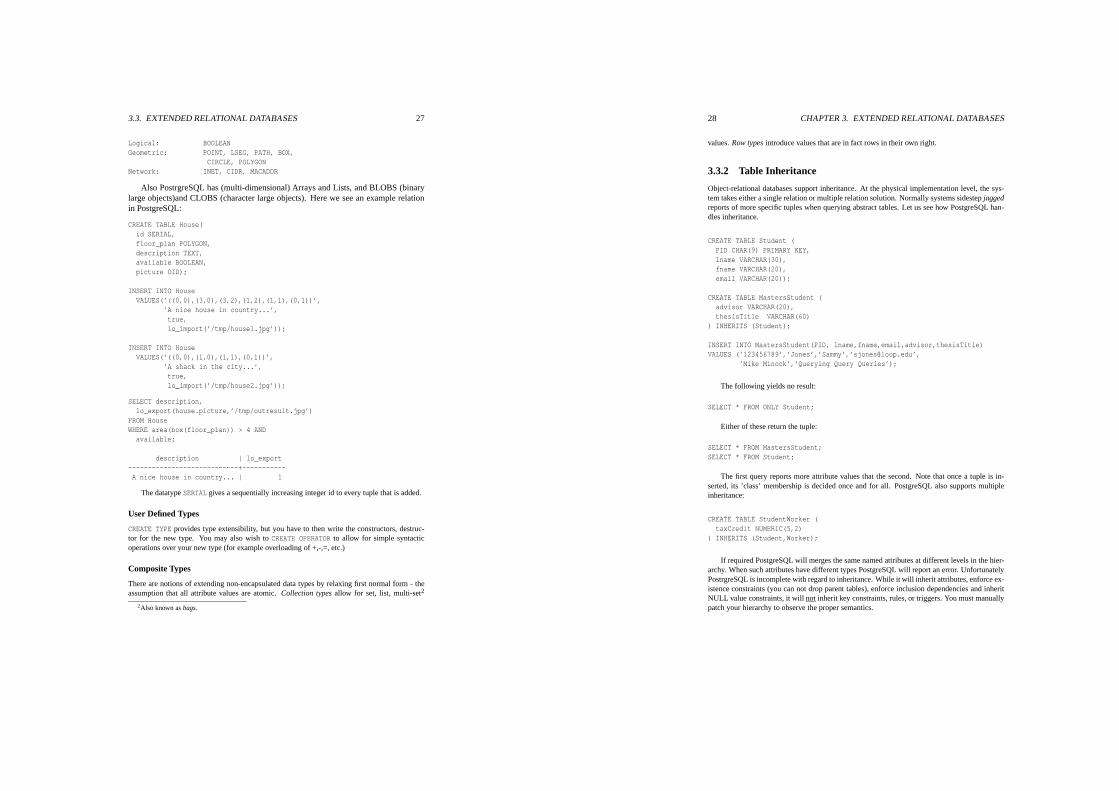
3.3. EXTENDED RELATIONAL DATABASES 27
Logical: BOOLEANGeometric: POINT, LSEG, PATH, BOX,
CIRCLE, POLYGONNetwork: INET, CIDR, MACADDR
Also PostrgreSQL has (multi-dimensional) Arrays and Lists, and BLOBS (binarylarge objects)and CLOBS (character large objects). Here we see an example relationin PostgreSQL:
CREATE TABLE House(id SERIAL,floor_plan POLYGON,description TEXT,available BOOLEAN,picture OID);
INSERT INTO HouseVALUES(’((0,0),(3,0),(3,2),(1,2),(1,1),(0,1))’,
’A nice house in country...’,true,lo_import(’/tmp/house1.jpg’));
INSERT INTO HouseVALUES(’((0,0),(1,0),(1,1),(0,1))’,
’A shack in the city...’,true,lo_import(’/tmp/house2.jpg’));
SELECT description,lo_export(house.picture,’/tmp/outresult.jpg’)
FROM HouseWHERE area(box(floor_plan)) > 4 ANDavailable;
description | lo_export----------------------------+-----------A nice house in country... | 1
The datatype SERIAL gives a sequentially increasing integer id to every tuple that is added.
User Defined Types
CREATE TYPE provides type extensibility, but you have to then write the constructors, destruc-tor for the new type. You may also wish to CREATE OPERATOR to allow for simple syntacticoperations over your new type (for example overloading of +,-,=, etc.)
Composite Types
There are notions of extending non-encapsulated data types by relaxing first normal form - theassumption that all attribute values are atomic. Collection types allow for set, list, multi-set2
2Also known as bags.
28 CHAPTER 3. EXTENDED RELATIONAL DATABASES
values. Row types introduce values that are in fact rows in their own right.
3.3.2 Table Inheritance
Object-relational databases support inheritance. At the physical implementation level, the sys-tem takes either a single relation or multiple relation solution. Normally systems sidestep jaggedreports of more specific tuples when querying abstract tables. Let us see how PostgreSQL han-dles inheritance.
CREATE TABLE Student (PID CHAR(9) PRIMARY KEY,lname VARCHAR(30),fname VARCHAR(20),email VARCHAR(20));
CREATE TABLE MastersStudent (advisor VARCHAR(20),thesisTitle VARCHAR(60)
) INHERITS (Student);
INSERT INTO MastersStudent(PID, lname,fname,email,advisor,thesisTitle)VALUES (’123456789’,’Jones’,’Sammy’,’[email protected]’,
’Mike Minock’,’Querying Query Queries’);
The following yields no result:
SELECT * FROM ONLY Student;
Either of these return the tuple:
SELECT * FROM MastersStudent;SELECT * FROM Student;
The first query reports more attribute values that the second. Note that once a tuple is in-serted, its ’class’ membership is decided once and for all. PostgreSQL also supports multipleinheritance:
CREATE TABLE StudentWorker (taxCredit NUMERIC(5,2)
) INHERITS (Student,Worker);
If required PostgreSQL will merges the same named attributes at different levels in the hier-archy. When such attributes have different types PostgreSQL will report an error. UnfortunatelyPostrgreSQL is incomplete with regard to inheritance. While it will inherit attributes, enforce ex-istence constraints (you can not drop parent tables), enforce inclusion dependencies and inheritNULL value constraints, it will not inherit key constraints, rules, or triggers. You must manuallypatch your hierarchy to observe the proper semantics.

3.3. EXTENDED RELATIONAL DATABASES 29
3.3.3 Active DatabasesTriggers are Event-Condition-Action (ECA) rules. Triggering events typically include insert,delete and update on a tuple (or table). For example external ’cron jobs’ engage triggers throughinsertions into tables. Conditions are usually predicates that may be evaluated over databasetables. Finally actions may either be SQL updates, external routines or stored procedures.
Triggers in the general sense are represented in PostgreSQL by either a TRIGGER or aRULE.The distinction between a rule and a trigger is that a rules have SQL statements as their actionswhereas triggers make calls to arbitrary procedures.
CREATE RULE integcon1 ASON INSERT TO OwnsWHERE NOT EXISTS(SELECT *FROM AssetWHERE Asset.symbol = new.asset)
DO INSTEAD NOTHING;
CREATE TRIGGER check_criticalAFTER INSERT OR UPDATE ON reactor_statusFOR EACH ROWEXECUTE PROCEDURE check_meltdown(new.temp, old.temp);
3.3.4 Stored ProceduresServer side functions improve performance and promote uniformity. There are already a largenumber of functions built in (issue \df) to list them all.
CREATE FUNCTION distance(numeric, numeric, numeric, numeric)RETURNS float8AS ’Select sqrt(($1 - $3)ˆ2 + ($2 - $4)ˆ2);’LANGUAGE ’sql’;
Note that the languages ’C’, ’JAVA’, ’PLPGSQL’ must be added with createlang commandline operation.
3.3.5 Linear RecursionPostgreSQL does not have any linear recursive features, but linear recursion is a part of the SQL1999 standard. To illustrate consider the table
PART_TABLE(Part1, Part2)
where Part1 contains Part2 as a component. For example “Volvo-121” contains “XY-Motor”.
Now let us consider the bill of materials type query: “give all the parts in a Volvo-121” Thisis solved with the following recursive query:
WITH RECURSIVEBILL_MATERIAL (Part1, Part2) AS(SELECT Part1,Part2FROM PART_TABLE
30 CHAPTER 3. EXTENDED RELATIONAL DATABASES
WHERE Part1 = ’Volvo-121’UNION ALL
SELECT PART_TABLE(Part1), PART_TABLE(Part2)FROM BILL_MATERIAL, PART_TABLEWHERE PART_TABLE.Part1 = BILL_MATERIAL(Part2))
SELECT * FROM BILL_MATERIALORDER BY Part1, Part2;
3.4 Semantically Suspect ExtensionsThe following extensions are more radical with respect to the basic relational model. Thus,from the point of view of this book, these extensions should be prohibited or at least stronglydiscouraged.
3.4.1 The Nested Model
The full generalization of collection and row types leads to the notion of the nested relationalmodel. The nested relational model gives a well-founded treatment of row and set collectiontypes. Essentially in the nested model we may ’nest’ an entire relation within an attribute. It isbest to consider an example:
MovieList = (list#, Movies)Movies = (title, year, director, Actors, Genres)Actors = (name)Genres = (genre)Seen = (person, Titles)Titles = (title)
list# Movies
title year director Actor Genres
person
actor genres
Titles
title
Seen
MovieList
1 Star Wars 1977 Lucas M. HamilH. Ford
Sci FiAdventure
1980Empire Lucas M. Hamil
H. Ford
Sci Fi
Adventure
Mike Start Wars
Empire
A nested attribute may be a multi-valued composite attribute (e.g. Movies), or a multi-valued simple attribute (e.g. Genres). Some models specifically treat single valued compos-ite attributes, but we will not. In the nested model we have external relational schemas (e.g.MovieList, Seen), internal relational schemas (e.g. Movies, Actors, Genres, Titles), and

3.5. BIBLIOGRAPHICAL AND HISTORICAL REMARKS 31
simple attributes (e.g. list#, title, year, director, name, person, genre). The nestedrelations represent independent information.
How do you represent the M:N relationship between people and directors of the movies thatthey have seen? This is difficult to capture in a hierarchical structure. But nested model is strictlymore expressive than relational – so just do it the standard way at the proper level of nesting.
The operator UNNEST flattens the Seen relation UNNESTTitles � � Title � Seen. This yieldthe first normal form relation with the attributes person and title. A similar operation:Πtitle � director UNNESTMovies � � title � director � MovieList generates a table with the attributes titleand director. These two tables may in turn be joined to form the table with attributes personand director.
We may also nest normal relations to a nested schema. From the flat tableSeenFlat(person,title) we build the Seen table through: NESTT IT LES � � T IT LE �� SeenFlat �
The operator NEST groups together the tuples with the same value for attributes not specified inthe NEST operation. This is similar to the GROUP BY construct in SQL.
3.4.2 Reference Types
OIDs
Every tuple receives an OID. This number in unique and immutable and thus identifies the tuple.
select oid,* from transactions;oid | tnum | items
-------+------+-------------19166 | 55 | {2,3,6,8}19173 | 56 | {6,7,22,88}19191 | 57 | {2}
OIDs are generated across a database installation and thus are not sequential. Nor are OIDsbacked up by default. This could potentially lead to problems if one uses such OIDs as objectreferences to tuples.
3.5 Bibliographical and Historical RemarksSQL was first specified in the 1970s SQL-86 (SQL1) was made an ANSI standard with tables,columns, views, basic relational operations, some integrity constraints, language bindings toCOBOL, FORTRAN, C, etc.
SQL-92 (SQL2) was made an official ANSI/ISO standard and has enjoyed tremendous suc-cess. It includes assertions, bit data type, case, character sets, connection management, DATE-TIME, domains, dynamic SQL, enhanced constraints (referential integrity), get diagnostics,grouped operations, information schema, natural character sets, natural joins (inner and outer),row and table constraints, schema manipulation, sub-queries in check clauses, table constraints,temporary tables, transactions, union and intersect.
SQL3 has had a slow, stormy and confused birth. But it has been born. The problem has beenthat proprietary approaches abound3 . It is unlikely that the Industry will converge. Additionallythe new names are now SQL1999 and subsequent improvements will be SQL200n. SQL1999and SQL200n are backward-compatible with SQL2.
3For example Informix offers a set of ’data blades’ and Oracle a set of ’catridges’ that, in essense, aresimply extended data types.
32 CHAPTER 3. EXTENDED RELATIONAL DATABASES
3.6 Exercises1. Assume the following nested definitions:
Person = (PersonNumber, Name, Age)HasJob = (PersonNumber, Job)Job = (Title, Duration)Duration = (StartYear, EndYear)
a. Name all of the external relations, internal relations, simple attributes in theschema above.
b. Using nested relational algebra, retrieve the person names for all those who haveworked as ’doctors’.
c. Using nested relational algebra retrieve the person name for those who worked as’singers’ in 1979.

Chapter 4
Temporal Databases
We have allowed for TIME and DATE attributes in our schemas. So we already have some expe-rience with time in databases. Still it is necessary to develop some general concepts around thedeeper modeling of temporal data. For example how would we support the following applica-tions:
� Health-care: Does this patient have any record of heart ailments? What about a familyhistory?
� Insurance: When is a policy in effect? Is a particular type of accident covered over aspecific period?
� Reservation Systems: When does a reservation expire?
� Scientific Databases: When was a measurement taken?
� Fraud Detection: Does a specific pattern of transactions indicate money laundering istaking place?
A common requirement for many temporal applications is the need to maintain an entirehistory of the changes to a tuple or object. Often we need to be able to support queries thatenable us to view ‘the state’ at any time in the past. We might also need to support more timebased queries as well. For example we might need to answer the query “Give the bank accountswhich had over a 1000% increase which was held for less than 2 days”. The technique by whichto do this is tuple versioning.
4.1 Time Representation
Under the non-relativistic, discrete case, time is an independent dimension arranged usuallyordered as sequence of points of some fixed granularity. For most applications this granularityis a second, a day, or a year, but they could just as easily be milli, micro, nano or pico seconds orcenturies,millenia, millions or billions of years.
Some, who want to respect the continuity of time, will speak in terms of the inter-pointdurations (termed a chronon) instead of points. Events occurring at the same point (or withinthe same chronon) will be seen as simultaneous. In any temporal application we speak of thegranularity as being the duration of a chronon. We speak of a duration as being an integernumber of chronons.
33
34 CHAPTER 4. TEMPORAL DATABASES
4.1.1 Calendar
A calendar is relative to a reference point and organizes time into different time units for con-venience. Some choices are Gregorian, Chinese, Islamic, Hindu, Jewish or Coptic. Of coursewe use the Gregorian calendar with its 12 irregular months and its extra day every fourth year1
Within SQL we have the DATE, TIME, and TIMESTAMP types, though their printed format maydiffer based on local convention.
� DATE (YYYY-MM-DD)
� TIME (HH:MM:SS)
� TIMESTAMP DATE and TIME together
4.1.2 Point and Interval Events
An event is an association between a fact and a given time value. Point events are associatedwith a single time points (or chronos). Interval events are associated with all the time points (orchronos) that lie between a beginning and an end time point inclusive of the start point, but notthe end time2
4.2 Valid Time and Transaction Time
There are two possible interpretations of the time value associated with a recorded fact: validtime or transaction time. Valid time represent the time the fact actually holds in the real world.Transaction time represents the time that the fact holds in the database. Some databases use thefirst notion (valid time database), some use the second (transaction time database) and some useboth time dimensions (bitemporal databases).
4.2.1 Valid Time Databases
Assuming that a tuple within a normal, non-temporal database records that a given fact is true inthe real world, then all that is needed to specify the interval over which fact is true is to supply avalid start time(VST) and a valid end time(VET). Thus all that is needed to make a non-temporaldatabase into a valid time database is to extend each tuple with the VST and VET attributes. Thusthe non-temporal schema:
LivesAt(personNumber, street, city, state)
becomes
LivesAt(personNumber, street, city, state, VST, VET)
We see here an example instance of this relation:
001, 122 Ford st., Chicago, IL, JAN-01-1989, MAR-16-1999001, 334 2nd st. , Los Angeles, CA, APR-12-1999, now
1With occasional leap seconds inserted at the beginning of January 1st.2By adopting this convention, we may have intervals meet exactly, but not overlap.

4.2. VALID TIME AND TRANSACTION TIME 35
The currently true fact has its valid end-time set to the special temporal variable now3.The total key now includes the time period values. A non-intersecting valid time points con-
straint may need to be observed as well. Also non-temporal keys may need to hold continuously,without gaps. In SQL2 this must be implemented using assertions. Most simple operations onrelations will need to be enclosed within transactions and must follow strict protocols.
Inserts
Inserts are straight forward and simply involve specifying the VST. Thus we may insert:
002, 10 Grant st., Lansing, MI, FEB-01-1995, now
Updates
On updates the system should close the current version and create a new version with the updatedvalues. So if person numbered 001 moves from LA to Austin in May 2003, we may alter thevalue now to MAY-12-2003 and add a tuple:
001, 10 State st., Austin, TX, MAY-12-2003, now
Note that one needs to state the valid time of the update and that relying on the current dateis often inaccurate; the update would need to be carried out precisely when person 001 arrivedin Austin. In other words often an update is a pro-active or retroactive update, but rarely is it asimultaneous update.
Deletes
On deletes one just closes the current version.
4.2.2 Transaction Time Databases
In a transaction time database, the actual state of the database through time is what may berecovered - unlike a valid time database where the state of the world is what is recorded. Thesedatabases are also called rollback databases. Such databases are useful in applications where wehave simultaneous updates - such as in many financial domains.
The treatment is almost identical to that for valid time databases. The difference howeveris that instead of valid start and end times we have transaction start times(TST) and transactionend times(TET). In addition the special constant now is replaced by the symbol uc - meaning untilchanged.
4.2.3 Bitemporal Databases
Sometimes we need to represent both transaction and valid time together. Tuples with TET as uc,represent currently valid information. The current version has TET = uc and VET = now.
3Often, in practice, one may use the value DEC-31-9999.
36 CHAPTER 4. TEMPORAL DATABASES
Inserts
Job(P#, Pos, Sal, VST, VET, TST, TET)13, CEO, 500k, 06-01-1999, now , 05-12-1999, uc
Here we see the insert if the 13th employee, a CEO into a small high tech company. Thetransaction was performed on May 12th and the contract terms are that the CEO is to start onJune 1st.
More abstractly, to insert an employee, create the tuple and set TST to the current time, andthe VST to whatever the valid start time should be, and the TET to uc and the VET to now.
Updates
Based on the semantics of bitemporal databases, no attributes may be changed on any tuple ex-cept TET on tuples with TET = uc. For this reason Bitemporal databases are sometimes referredto as append only databases.
Assuming that the CEO, as his first concrete action, decides to raise employee number 13salary by 400k, effective immediately. Further assume that this action is carried out on June13th. The resulting database contains:
Job(P#, Pos, Sal, VST, VET, TST, TET)13, CEO, 500k, 06-01-1999, now , 05-12-1999, 06-13-199913, CEO, 500k, 06-01-1999, 06-13-1999, 06-13-1999, uc13, CEO, 900k, 06-13-1999, now , 06-13-1999, uc
Assuming that v is the tuple which we are changing the salary of, newSalary is the newsalary, vst is when the new salary becomes effective, and tst is precisely when the function isexecuted, the following code performs our update:
changeSalary(v, newSalary){v2 = copy (v);v2.vet = vst; //immediately prior to VTv2.tst = tst); //transaction timev2.tet = uc;insert v2; // Current ’old’ version with old salary
v3 = copy (v);v3.vst = vst;v3.vet = now;v3.salary = newSalary;v3.tst = tst;v3.tet = uc;insert v3; // Current ’new’ version with new salary
v.tet = tst; // Non current version with old salary terms}
Deletes
In February of 2003 the board of directors finally wises up and realizes that the CEO has notbeen at work that year. They decide to fire the CEO effective December 31st, 2002. This givesthe database state:

4.3. ALLEN’S INTERVAL ALGEBRA 37
Job(P#, Pos, Sal, VST, VET, TST, TET)13, CEO, 500k, 06-01-1999, now , 05-12-1999, 06-13-199913, CEO, 500k, 06-01-1999, 06-13-1999, 06-13-1999, uc13, CEO, 900k, 06-13-1999, now , 06-13-1999, 02-10-200313, CEO, 900k, 06-13-1999, 12-31-2003, 02-10-2003, uc
More abstractly to delete the current valid tuple v, create a copy v2 of v. Set the VET to theproper end-time and the TST to the time of the transaction and the TET to uc. Then simply setTET on v from uc to the time of the delete transaction.
Note that a history of all the changes are computed. So I can, one year later, knock Smith’ssalary up for the last year. And the record of me doing this, and the previous and now updatedvalues of Smith’s salary will be kept.
Implementation and Other Issues
We could keep all the information is a single table, or we could keep the currently valid infor-mation in one table and the history a second. This later option, though complicated by joins andtriggers, is more efficient.
4.3 Allen’s Interval AlgebraThe interval x starts at x
� and ends at x� . (x � � x� ). Likewise the interval y starts at y
� andends at y� . (y � � y� )
Relation Symbol Example Conditions
x before y � XXX x� � y �
y after x � YYYx meets y m XXXX x� � y �
y met-by x m� YYYYx overlaps y o XXXX x � � y � � x� ,y overlaped-by x o� YYYY x� � y�
x during y d XX x � � y � ,y includes x d� YYYY x� � y�
x starts y s XXXX x � � y � ,y started-by x s� YYYYYYYY x� � y�
x finishes y f XXXX x� � y�
y finished-by x f� YYYYYYYY x � � y �
x equals y � XXXX x � � y � ,YYYY x� � y�
The general problem of determining the satisfiability of a set of n temporal relation state-ments in Allen’s Algebra is intractable.
Note that set operations on intervals, leads to an algebra of temporal elements. Coalescinginsures uniqueness of temporal elements.
4.4 Time Series DataTime series records data-values over a predetermined sequence of data points on a calendar.Queries are often temporal aggregation queries over larger granularities than the time seriescalendar.
38 CHAPTER 4. TEMPORAL DATABASES
4.5 Bibliographical and Historical RemarksTSQL2 is an extension to SQL-92 that allows temporal tables to be specified in the DDL. Theimplementation of the temporal aspects are thus largely hidden from the user.
CREATE TABLE AS VALID STATE <GRANULARITY>CREATE TABLE AS VALID EVENT <GRANULARITY>CREATE TABLE AS TRANSACTION
The operators INCLUDES, INCLUDED_IN, OVERLAPS, BEFORE, AFTER, MEETS_BEFORE,MEETS_AFTER are added to SQL.
[X.tst,x.tet] OVERLAPS [2001-9-0,2001-9-10]

4.6. EXERCISES 39
4.6 Exercises1. Sale(SNum, Cust, Item, Price, Date, TST, TET)
001, Stinky, A-XT, 1,200 USD, 06-23-89, 06-23-89, uc...
In SQL (or Datalog if you wish):
a.) Give the sales that did not get revised in any way.
b.) Give the sales that had a price revised downward.
c.) Give the sales that were canceled.
d.) Show the relevant tuples after we update the name ’Stinky’ to the name ’Corn Fed’on 01-01-93.
2. CashValue(AccountNumber, Cash, TST, TET)001 100 USD Dec-1992, uc002 1000 USD Apr-2000, uc...
In SQL (or Datalog if you wish):
a. Give the account numbers that currently have more than 1000 USD.
b. Give the account numbers that were opened in Apr-2000.
c. Give the account numbers that were active, then closed, and then were reactivated.
d. Give the account numbers that had less than 1000 USD, were then immediatelyraised to over a 1,000,000 USD, and were then closed within the next month.
3. For the events x,y, and z the following expression in Allen’s Algebra is satisfiable: � x �
y �� � z d y �� � x o z): _____ ___.
4. (FossilNum, Description , Species, Dated, TST, TET)001 Skull Fragment, Homo Erectus, 3500 , 1946, 1978001 Skull Fragment, Homo Habulus, 3780 , 1979, uc002 Leg Bone Home Sapien, 450, 1996, uc
...
In SQL (or Datalog if you wish):
a. Give the collection of fossils thought to belong to Homo Sapiens as of 1979.
b. Give the fossils that have been classified to two of more different species at differenttimes.
c. In pseudo code show how to update all the Skull fragments dated before 500 andclassified to Homo Sapien, to be classified to Homo Erectus. Assume this transac-tion to be carded out in 2002.
40 CHAPTER 4. TEMPORAL DATABASES
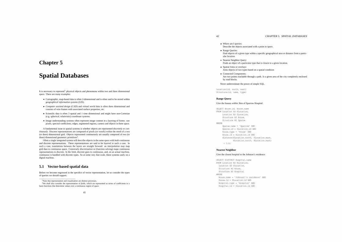
Chapter 5
Spatial Databases
It is necessary to represent1 physical objects and phenomena within two and three dimensionalspace. There are many examples:
� Cartographic, map-based data is often 2-dimensional and is often said to be stored withingeographical information systems (GIS).
� Computer assisted design (CAD) and virtual world data is often three dimensional andconsists of wire frames with associated surface properties, etc.
� Scientific data is often 3 spatial and 1 time dimensional and might have non-Cartesian(e.g. spherical, relativistic) coordinate systems.
� Image understanding systems often represent image content in a layering of forms: rawpixels, spectral coefficients, edges, segmented regions, camera and objects in three space.
A fundamental issue in spatial systems is whether objects are represented discretely or con-tinuously. Discrete representations are composed of pixels (or voxels) within the mesh of a two(or three) dimensional grid. Objects represented continuously are usually composed of two (orthree) dimensional geometric primitives2.
Often a single integrated system will describe objects in the same space with both continuousand discrete representations. These representations are said to be layered in such a case. Insuch a case, translations between the layers are straight forward: an interpolation may mapgrid data to continuous space. Conversely discretization or (function solving) maps continuousrepresentations to discrete. In the limit, discrete goes to continuous, and, on an actual machine,continuous is handled with discrete types. So at some very fine scale, these systems unify on adigital machine.
5.1 Vector-based spatial data
Before we become engrossed in the specifics of vector representation, let us consider the typesof queries we should support.
1Note that representation and visualization are distinct processes.2We shall also consider the representation of fields, which are represented as series of coefficients to a
basis functions that determine values over a continuous region of space.
41
42 CHAPTER 5. SPATIAL DATABASES
� Where am I queries:Describe the objects associated with a point in space.
� Range Queries:Find objects of a given type within a specific geographical area or distance from a partic-ular location.
� Nearest Neighbor Query:Finds an object of a particular type that is closest to a given location.
� Spatial Joins or overlays:Joins objects of two types based on a spatial condition
� Connected Components:Are two points reachable through a path. Is a given area of the city completely enclosedby road blocks.
Never underestimate the power of simple SQL.
Location(id, north, east)Structure(id, name, type)
Range Query
Give the houses within 3km of Sparrow Hospital:
SELECT House.id, House.nameFROM Location AS HLocation,
Location AS SLocation,Structure AS House,Structure AS Sparow
WHERESparow.name = ’Sparrow’ ANDSparow.id = SLocation.id ANDHouse.type = ’House’ ANDHouse.id = HLocation.id ANDdistance(SLocation.north, SLocation.east,
HLocation.north, HLocation.east)< 3.0;
Nearest Neighbor
Give the closest hospital to the Johnson’s residence:
SELECT DISTINCT Hospital.nameFROM Location AS HLocation,Location AS SLocation,Structure AS House,Structure AS Hospital
WHEREHouse.name = ’Johnson\’s residence’ ANDHouse.id = HLocation.id ANDHospital.type = ’Hospital’ ANDHospital.id = SLocation.id AND
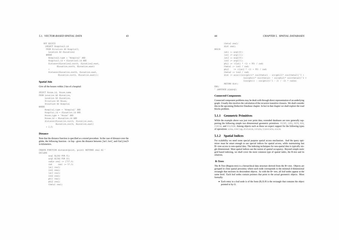
5.1. VECTOR-BASED SPATIAL DATA 43
NOT EXISTS(SELECT Hospital2.idFROM Structure AS Hospital2,Location AS SLocation2
WHEREHospital2.type = ’Hospital’ ANDHospital2.id = SLocation2.id ANDDistance(SLocation2.north, SLocation2.east,
HLocation.north, HLocation.east)<Distance(SLocation.north, SLocation.east,
HLocation.north, HLocation.east));
Spatial Join
Give all the houses within 2 km of a hospital:
SELECT House.id, House.nameFROM Location AS HLocation,
Location AS SLocation,Structure AS House,Structure AS Hospital
WHEREHospital.type = ’Hospital’ ANDHospital.id = SLocation.id ANDHouse.type = ’House’ ANDHouse.id = HLocation.id ANDdistance(SLocation.north, SLocation.east,
HLocation.north, HLocation.east)< 2.0;
Distance
Note that the distance function is specified as a stored procedure. In the case of distance over theglobe, the following function - in lisp - gives the distance between� lat1
�
lon1 � and� lat2
�
lon2 �
in kilometers.
CREATE FUNCTION distance(point, point) RETURNS real AS ’DECLARE
arg1 ALIAS FOR $1;arg2 ALIAS FOR $2;radie real := 1737.4;rad real := 57.3;lat1 real;lon1 real;lat2 real;lon2 real;phi1 real;phi2 real;theta1 real;
44 CHAPTER 5. SPATIAL DATABASES
theta2 real;dist real;
BEGINlat1 := arg1[0];lon1 := arg1[1];lat2 := arg2[0];lon2 := arg2[1];phi1 := ((lat1 * -1) + 90) / rad;theta1 := lon1 / rad;phi2 := ((lat2 * -1) + 90) / rad;theta2 := lon2 / rad;dist := acos(((sin(phi1)* cos(theta1) - sin(phi2)* cos(theta2))ˆ2 +
(sin(phi1)* sin(theta1) - sin(phi2)* sin(theta2))ˆ2 +(cos(phi1) - cos(phi2))ˆ2 - 2) / -2) * radie;
RETURN dist;END;’ LANGUAGE plpgsql;
Connected Components
Connected component problems may be dealt with through direct representation of an underlyinggraph. Usually this involves the calculation of the recursive transitive closures. We shall considerthis in the upcoming Deductive Database chapter. In fact in that chapter we shall explore the roadblocks problem.
5.1.1 Geometric PrimitivesWhile the example above was just over point data, extended databases are now generally sup-porting the following simple two dimensional geometric primitives: POINT, LSEG, PATH, BOX,CIRCLE, and POLYGON. Among objects such as these we expect support for the following typesof operations: area, overlap, distance, rotate, translate, scale.
5.1.2 Spatial IndicesFor scalability we need some special purpose spatial access mechanism. And the query opti-mizer must be smart enough to use special indices for spatial access, while maintaining fastB+-tree access to non-spatial data. The indexing techniques for non-spatial data is typically sin-gle dimensional. Most spatial indices use the notion of spatial occupancy. Beyond simple staticgrid based indexing, we shall cover the most common type of spatial index, the R-tree and itsrelatives.
R-Trees
The R-Tree (Region-tree) is a hierarchical data structure derived from the B+-tree. Objects aregrouped in close spatial proximity where each node corresponds to the minimal d-dimensionalrectangle that encloses its descendent objects. As with the B+ tree, all leaf nodes appear at thesame level. Each leaf nodes contain pointers that point to the actual geometric objects. Moreformally:
� Each entry in a leaf node is of the form (R,O) R is the rectangle that contains the objectpointed to by O.

5.1. VECTOR-BASED SPATIAL DATA 45
� Each entry in an interior node is a 2-tuple of form (R,P) where R is the smallest rectanglethat spatially contains the children on the descendents of the node pointed to by P.
� Aside from the root, all nodes must have more than some minimum number m entries.An R-tree is said to be of order (m,M) where m � � M � 2 � .
In the following example we have a 2-3 R-Tree over 8-objects.
R1 R2
R3 R5 R6R4
1 2 3 4 5 6 7 8
R2
R4
R5
R6
R1
1 2
34
5
6
7
8
R3
Insertion is made by traversing down the tree, picking the path that requires the minimumamount of enlargement (in terms of area) of the rectangles in each internal node. If there isoverfill of a leaf, node then we require node splitting. Node splitting is complex in R-Trees, butin general we wish to minimize the total area of the covering rectangles. Deletion cause an objectto be removed from a leaf node. Under-fill precipitates the re-insertion of the objects. Accessingpoints and regions is straight-forward. But the search may have to follow multiple paths.
PostgreSQL supports R-trees. The following command builds an index for the aboveschema.
create index HouseRtree on House using rtree (floor_plan);
The index will be used when certain operators are used in the query. For example a @ b(meaning a overlaps in b) and a << b (a is to the left of b) are used in the following query fororders of magnitude speed up.
46 CHAPTER 5. SPATIAL DATABASES
select *from House AS xwhere exists (select *from House ywhere y.floorplan @ ’(0,0),(100,0),(100,100),(0,100),(0,0)’
and y.floor_plan << x.floor_plan) and x.floorplan @ ’(0,0),(100,0),(100,100),(0,100),(0,0)’;
5.1.3 Affine TransformationsGive the set of two-dimensional points in our description of an object, we may apply affinetransformations to scale, translate (AKA move), or rotate the object.
Translation : ��
1 0 tx0 1 ty0 0 1
��
Scaling : ��
sx 0 00 sy 00 0 1
��
Rotation : ��
cos� θ �
� sin� θ � 0sin� θ � cos� θ � 0
0 0 1
��
A line segment, defined by endpoints (0,0) and (1,1) shrinks by 50%, rotates minus 45deg,and moves 4 units in the X direction and 2 units in the Y direction.
The endpoint (0,0) is transformed:
1 0 40 1 20 0 1
��� 71 71 0� 71 71 0
0 0 1
�� 5 0 0
0 5 00 0 1
��
001
����
355 355 4� 355 355 2
0 0 1
��
001
���
421
��
The endpoint (1,1) is transformed:
1 0 40 1 20 0 1
��� 71 71 0� 71 71 0
0 0 1
�� 5 0 0
0 5 00 0 1
��
111
����

5.2. GRID BASED SPATIAL DATA 47
��
� 355 � 355 4
� � 355 � 355 20 0 1
��
��
111
��
� ��
4 � 7121
��
Operations are often carried out relative to the centroid of the object. Thus the generalapproach is to: 1.) Find centroid of object; 2.) Translate each point defining the object such thatcentroid is on the origin. 3.) Apply scaling and rotation operations to each point defining theobject. 4.) Apply translation operations to each point defining the object. 5.) Re-translate objectback to original position of centroid.
5.2 Grid based spatial dataClearly two and three dimensional bit maps are the straight forward way to model grid-baseddata. In general they do not scale however. Not only are the space requirements large, but ’set’operations that intersect, subtract, and union bit maps are time expensive as well. The classicaltechnique to address these shortcomings are quad-trees.
5.2.1 Quad-treesTwo dimensional quad-trees successively sub-divide a two dimensional grid into four equal sizedquadrants. If quadrants are not homogeneous, then they are sub-divided recursively. In the worstcase this sub-division stops when the 1 � 1 blocks in the granularity of the grid is reached - acondition of homogeneity by definition. Quad trees generalize to three dimensions (and greater)in the obvious way.
1
2 3
4 56
7 8
9 1011
1
2 3 4 5
6
7 8 9 10
11
12 13
1415 16
17 18
19 20
21 2223
24 25
12 13 14
15 16 17 1819 20 21 22
23 24 25
(0 ((1110) 1 (1000) 0) (000 (1101)) ((0001)000)
Quad-trees are a variable resolution method; the resolution is variable depending on whatis required. Quad-trees are origin sensitive. One may rapidly perform set operation betweenquad-trees as well.
48 CHAPTER 5. SPATIAL DATABASES
The Quad Tree complexity theorem states that The average number of nodes in the quadtree representation is O� p � q � for a 2qx2q image with perimeter p. In an 8 � 8 quad-trees wethus have q � 3 and p � 32, so we should have, on average, 35 nodes. The savings are not soimpressive. But for a 1024x1024 grid. A bit map gives 1MG pixels. A quad-tree gives (onaverage) a 1024 * 4 + 10 nodes.
5.3 Field DataSometimes we have a continuous function that has a value for each point in space (E.g. Ther-mospheric Model or Heart models). In such a situation we have a set of basis functions pairedwith a set of coefficients (the data). The coefficients have been found through one technique oranother and the ’query’ is the solution of the (coefficient weighted) basis functions at a particularpoint. Common basis functions include, Fourier series, wavelets, Legendre polynomials, etc.Truncation schemes save time and space.
5.4 Bibliographical and Historical RemarksThere are many variations of R-Trees and Quad trees discussed in Sammet’s work on spatialdata. There is a special type of R-Tree named the packed R-Tree. Packed R-Trees are used forstatic arrangements of objects. Packed R-Trees are just R-Trees that are optimally full and arebuild the R-tree bottom up, relying on close spatial proximity. In R+ trees overlap is not allowedin the bounding rectangles of interior nodes. And a object that spans two interior node rectangleswill have a leaf node entry under both internal nodes. The height of tree grows quite a bit andkeeping nodes greater than 1/2 full is costly.
ARCGIS is a popular platform for doing GIS. The tool could perhaps be best described as“photoshop for map based data.”. However, from a database perspective the system has inter-operability problems. The OpenGIS http://www.opengis.org/ effort is probably a more pro-ductive and less expensive alternative.

5.5. EXERCISES 49
5.5 Exercises
Figure 5.1: EER Diagram
1. Following an “upper left quadrant and clockwise” fill-in protocol, fill the image abovewith the quad-tree:
(1 0 (1 0 (1 0 1 0) 1) (1 0 0 1))
2. Draw an image that causes a worst-case quad tree.
3. Justify (or refute) the following claim: “Intersection between two images is (on average)faster, if the two images are represented as quad-trees rather than as simple bitmaps.”
50 CHAPTER 5. SPATIAL DATABASES
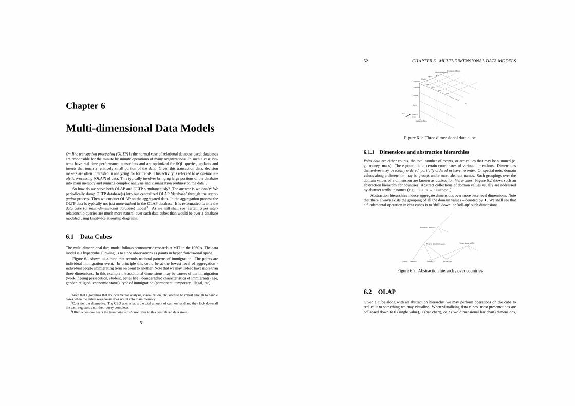
Chapter 6
Multi-dimensional Data Models
On-line transaction processing (OLTP) is the normal case of relational database used; databasesare responsible for the minute by minute operations of many organizations. In such a case sys-tems have real time performance constraints and are optimized for SQL queries, updates andinserts that touch a relatively small portion of the data. Given this transaction data, decisionmakers are often interested in analyzing for for trends. This activity is refereed to as on-line an-alytic processing (OLAP) of data. This typically involves bringing large portions of the databaseinto main memory and running complex analysis and visualization routines on the data1.
So how do we serve both OLAP and OLTP simultaneously? The answer is we don’t2 Weperiodically dump OLTP database(s) into our centralized OLAP ’database’ through the aggre-gation process. Then we conduct OLAP on the aggregated data. In the aggregation process theOLTP data is typically not just materialized in the OLAP database. It is reformatted to fit a thedata cube (or multi-dimensional database) model3. As we will shall see, certain types inter-relationship queries are much more natural over such data cubes than would be over a databasemodeled using Entity-Relationship diagrams.
6.1 Data Cubes
The multi-dimensional data model follows econometric research at MIT in the 1960’s. The datamodel is a hypercube allowing us to store observations as points in hyper dimensional space.
Figure 6.1 shows us a cube that records national patterns of immigration. The points areindividual immigration event. In principle this could be at the lowest level of aggregation -individual people immigrating from on point to another. Note that we may indeed have more thanthree dimensions. In this example the additional dimensions may be causes of the immigration(work, fleeing persecution, student, better life), demographic characteristics of immigrants (age,gender, religion, economic status), type of immigration (permanent, temporary, illegal, etc).
1Note that algorithms that do incremental analysis, visualization, etc. need to be robust enough to handlecases when the entire warehouse does not fit into main memory.
2Consider the alternative. The CEO asks what is the total amount of cash on hand and they lock down allthe cash registers until their query completes.
3Often when one hears the term data warehouse refer to this centralized data store.
51
52 CHAPTER 6. MULTI-DIMENSIONAL DATA MODELS
1980
1982
Imigrated too
Afganistan
Albania
Algeria
American Samoa
Afganistan
Albania
Algeria
AmericanSamoa
Emigrated From
Year
(y)
(x)
(z)
view
1981
1983
Figure 6.1: Three dimensional data cube
6.1.1 Dimensions and abstraction hierarchies
Point data are either counts, the total number of events, or are values that may be summed (e.g. money, mass). These points lie at certain coordinates of various dimensions. Dimensionsthemselves may be totally ordered, partially ordered or have no order. Of special note, domainvalues along a dimension may be groups under more abstract names. Such groupings over thedomain values of a dimension are known as abstraction hierarchies. Figure 6.2 shows such anabstraction hierarchy for countries. Abstract collections of domain values usually are addressedby abstract attribute names (e.g. REGION = ’Europe’).
Abstraction hierarchies induce aggregate dimensions over more base level dimensions. Notethat there always exists the grouping of all the domain values – denoted by � . We shall see thata fundamental operation in data cubes is to ’drill down’ or ’roll-up’ such dimensions.
SWEDEN DENMARK
Treaty Group: NATO
Country:
Region: SCANDINAVIA
EUROPEContinent:
NORWAY
Figure 6.2: Abstraction hierarchy over countries
6.2 OLAP
Given a cube along with an abstraction hierarchy, we may perform operations on the cube toreduce it to something we may visualize. When visualizing data cubes, most presentations arecollapsed down to 0 (single value), 1 (bar chart), or 2 (two dimensional bar chart) dimensions,

6.2. OLAP 53
although attempts have been made to present data in higher dimensions. In figure 6.3 we see alldata integrated over all dimensions and collapsed to the single time dimension.
�����������
�����������
���������
���������
�������
�������
���������
���������
����
����
�������������
�������������
� � � � � �
�������������
���������������
���������������
���������������
���������������
���������
���������
2000
Number
1990
VISAS GRANTED TO SCANDINAVIAN STUDENTS TO STUDY IN NORTHAMERICA
500
1000
2000
1500
Figure 6.3: Collapsed to single dimensional vector
Consider the output from 3 dimensional cube to be a 2 dimensional spread sheet.
YEAR 1990 1991 ...COUNTRYDenmark 231 223 ...Iceland 11 22 ...Norway 452 454 ...Sweden 891 980 ...
Our bar chart above did the further aggregation (summing up) among Scandinavians coun-tries. Collapsing the results to a one dimensional array.
To transform an input data-cube into such a projection, we execute a sequence of elementaryoperations over the data cube. The three fundamental types of operations are presented below.
6.2.1 Pivot (rotation) operations
Consider that we have a paired down the initial hyper-cube to the student visas granted to Scan-dinavians to study in the countries of North America. A pivot is turning the cube (also calledrotation).
The results of these rotations result in six different faces of the cube being show. The numberof faces of a hyper-cube is the factorial of the number of its dimensions: A two-dimensional arrayhas two views, a three-dimensional cube has six, a four-dimensional hyper-cube has 24 and a fivedimensional hyper cube has 120 views, etc.
TO USA Canada MexicoDenmark 5600 1232 1102Iceland 234 112 89Norway 8903 798 211Sweden 12342 1984 1090
54 CHAPTER 6. MULTI-DIMENSIONAL DATA MODELS
6.2.2 Selection - slice (and dice)This shaves the Hyper Cube down to a smaller cube through applying a predicate. Slice namesthe value to project out along one of the dimensions. Dice names a group of values to project out- often by using an abstract attribute, value pair.
6.2.3 Roll-up/drill-downRoll-up names a grouping along one dimension and calls for aggregation along that grouping(e.g. Region. Note that often the role-up will be called over all the values along a dimensions( � ). This is the technique we use to reduce the dimension of a hyper-cube by one.
So for example if we role-up both the countries into the Scandinavians in the first spreadsheet we get:
YEAR 1990 1991 ...COUNTRYScandinavia 1781 1893
6.2.4 Operation SequencesWe built our graph of student visas in the nineties through the following operations over thehypercube:
HCUBE[x][y][z]...
Assume that our spread sheet view consists of x columns and y rows.
HCUBE = Immigration(Year, From, To, Cause, Gender,Age, Religion, Economic Status, Type)
PIVOT_TO(dim1,dim2,...)ROLLUP(abstractAttribute)DRILL-DOWN(abstractAttribute)SLICE(attribute = value)
6.3 ROLAP: Representing the Cube with RelationsEarly systems tended to implement the data cube directly. This is now to referred to as MOLAP,however beginning in the mid nineties, efforts were made to efficiently support such capabilitiesin relational databases. This is referred to as ROLAP.
In ROLAP: The relations are either FACT or DIMENSION Tables. One must be carefulabout what dimensions that data is indexed on. For example indexing on a key would lead tonon-interesting sparse cubes. Remember that the dimensions are interesting to the extent thatthere are relationships between them.
ROLAP schemas are star schemas, or snowflake schemas. Star schemas have the fact tableas a central table and dimension tables are joined with each corresponding dimension. So, forexample, we have the table:
Immigrants(Number, Year, From, To, Cause, Gender,Age, Religion, EconomicStatus, Type)
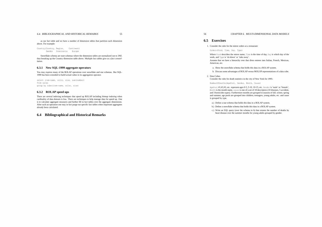
6.4. BIBLIOGRAPHICAL AND HISTORICAL REMARKS 55
as our fact table and we have a number of dimension tables that partition each dimensionabove. For example:
Country(Country, Region, Continent)Sweden Scaninavia Europe
Snowflake schema are start schemas where the dimension tables are normalized out to 3NF,thus breaking up the Country dimension table above. Multiple fact tables give us a fact constel-lation.
6.3.1 New SQL-1999 aggregate operatorsYou may express many of the ROLAP operations over snowflake and star schemas. But SQL-1999 has been extended to build actual cubes in its aggregation operator.
select item-name, color, size, sum(number)from salesgroup by cube(item-name, color, size)
6.3.2 ROLAP speed upsThere are several indexing techniques that speed up ROLAP including bitmap indexing whencardinality of data domain is low. There are techniques to help manage data for speed up. Oneis to calculate aggregate measures and further fill in fact tables over the aggregate dimensions.After such an operation one may in fact purge out specific fact tables when important aggregatesalready been calculated.
6.4 Bibliographical and Historical Remarks
56 CHAPTER 6. MULTI-DIMENSIONAL DATA MODELS
6.5 Exercises1. Consider the cube for the entree orders at a restaurant:
Orders(Food, Time, Day, Type)
Where Food describes the entree name, Time is the time of day, Day is which day of theweek, and Type is ’sit-down’ or ’take away’.
Assume that we have a hierarchy over that dives entrees into Italian, French, Mexican,American, etc.
a. Show the snowflake schema that holds this data in a ROLAP system.
b. Discuss some advantages of ROLAP versus MOLOP representations of a data cube.
2. Data CubesConsider the cube for death statistics in the city of New York for 1995:
NumberOfDeaths(AgePool, Gender, Month, Cause)
AgePool #1,#2,#3, etc. represent ages 0-5, 5-10, 10-15, etc. Gender is ’male’ or ’female’,Month is the month name, cause is one of a set of 18 descriptors (10 diseases, 5 accident,and 3 homicides types). Furthermore months are grouped in seasons of fall, winter, springand summer, age pools are grouped into children, teenagers, young adults, etc. and causeis grouped by type.
a.) Define a star schema that holds this data in a ROLAP system.
b.) Define a snowflake schema that holds this data in a ROLAP system.
c.) Write an SQL query (over the schema in b) that returns the number of deaths byheart disease over the summer months for young adults grouped by gender.
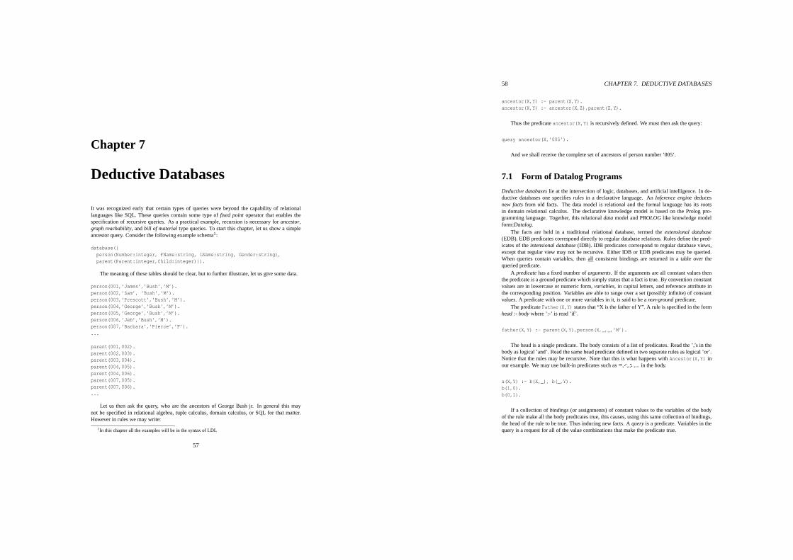
Chapter 7
Deductive Databases
It was recognized early that certain types of queries were beyond the capability of relationallanguages like SQL. These queries contain some type of fixed point operator that enables thespecification of recursive queries. As a practical example, recursion is necessary for ancestor,graph reachability, and bill of material type queries. To start this chapter, let us show a simpleancestor query. Consider the following example schema1:
database({person(Number:integer, FName:string, LName:string, Gender:string),parent(Parent:integer,Child:integer)}).
The meaning of these tables should be clear, but to further illustrate, let us give some data.
person(001,’James’,’Bush’,’M’).person(002,’Sam’, ’Bush’,’M’).person(003,’Prescott’,’Bush’,’M’).person(004,’George’,’Bush’,’M’).person(005,’George’,’Bush’,’M’).person(006,’Jeb’,’Bush’,’M’).person(007,’Barbara’,’Pierce’,’F’)....
parent(001,002).parent(002,003).parent(003,004).parent(004,005).parent(004,006).parent(007,005).parent(007,006)....
Let us then ask the query, who are the ancestors of George Bush jr. In general this maynot be specified in relational algebra, tuple calculus, domain calculus, or SQL for that matter.However in rules we may write:
1In this chapter all the examples will be in the syntax of LDL
57
58 CHAPTER 7. DEDUCTIVE DATABASES
ancestor(X,Y) :- parent(X,Y).ancestor(X,Y) :- ancestor(X,Z),parent(Z,Y).
Thus the predicate ancestor(X,Y) is recursively defined. We must then ask the query:
query ancestor(X,’005’).
And we shall receive the complete set of ancestors of person number ’005’.
7.1 Form of Datalog Programs
Deductive databases lie at the intersection of logic, databases, and artificial intelligence. In de-ductive databases one specifies rules in a declarative language. An Inference engine deducesnew facts from old facts. The data model is relational and the formal language has its rootsin domain relational calculus. The declarative knowledge model is based on the Prolog pro-gramming language. Together, this relational data model and PROLOG like knowledge modelform:Datalog.
The facts are held in a traditional relational database, termed the extensional database(EDB). EDB predicates correspond directly to regular database relations. Rules define the pred-icates of the intensional database (IDB). IDB predicates correspond to regular database views,except that regular view may not be recursive. Either IDB or EDB predicates may be queried.When queries contain variables, then all consistent bindings are returned in a table over thequeried predicate.
A predicate has a fixed number of arguments. If the arguments are all constant values thenthe predicate is a ground predicate which simply states that a fact is true. By convention constantvalues are in lowercase or numeric form, variables, in capital letters, and reference attribute inthe corresponding position. Variables are able to range over a set (possibly infinite) of constantvalues. A predicate with one or more variables in it, is said to be a non-ground predicate.
The predicate Father(X,Y) states that “X is the father of Y”. A rule is specified in the formhead :- body where ’:-’ is read ’if’.
father(X,Y) :- parent(X,Y),person(X,_,_,’M’).
The head is a single predicate. The body consists of a list of predicates. Read the ’,’s in thebody as logical ’and’. Read the same head predicate defined in two separate rules as logical ’or’.Notice that the rules may be recursive. Note that this is what happens with Ancestor(X,Y) inour example. We may use built-in predicates such as � , � , � ,... in the body.
a(X,Y) :- b(X,_), b(_,Y).b(1,0).b(0,1).
If a collection of bindings (or assignments) of constant values to the variables of the bodyof the rule make all the body predicates true, this causes, using this same collection of bindings,the head of the rule to be true. Thus inducing new facts. A query is a predicate. Variables in thequery is a request for all of the value combinations that make the predicate true.
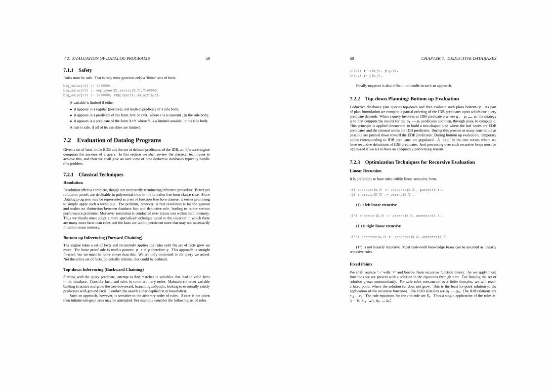
7.2. EVALUATION OF DATALOG PROGRAMS 59
7.1.1 SafetyRules must be safe. That is they must generate only a ’finite’ sets of facts.
big_salary(Y) :- Y>60000.big_salary(Y) :- employee(X),salary(X,Y),Y>60000.big_salary(Y) :- Y>60000, employee(X),salary(X,Y).
A variable is limited if either
� it appears in a regular (positive), not built-in predicate of a rule body.
� it appears in a predicate of the form X=c or c=X, where c is a constant , in the rule body.
� it appears is a predicate of the form X=Y where Y is a limited variable, in the rule body.
A rule is safe, if all of its variables are limited.
7.2 Evaluation of Datalog ProgramsGiven a set of facts in the EDB and the set of defined predicates of the IDB, an inference enginecomputes the answers of a query. In this section we shall review the classical techniques toachieve this, and then we shall give an over view of how deductive databases typically handlethis problem.
7.2.1 Classical Techniques
Resolution
Resolution offers a complete, though not necessarily terminating inference procedure. Better yetrefutation proofs are decidable in polynomial time in the function free horn clause case. SinceDatalog programs may be represented as a set of function free horn clauses, it seems promisingto simply apply such a technique. The problem, however, is that resolution is far too generaland makes no distinction between database fact and deductive rule, leading to rather seriousperformance problems. Moreover resolution is conducted over clause sets within main memory.Thus we clearly must adopt a more specialized technique tuned to the situation in which thereare many more facts than rules and the facts are within persistent store that may not necessarilyfit within main memory.
Bottom-up Inferencing (Forward Chaining)
The engine takes a set of facts and recursively applies the rules until the set of facts grow nomore. The basic proof rule is modus ponens: p � q, p therefore q. This approach is straightforward, but we must be more clever than this. We are only interested in the query we asked.Not the entire set of facts, potentially infinite, that could be deduced.
Top-down Inferencing (Backward Chaining)
Starting with the query predicate, attempt to find matches to variables that lead to valid factsin the database. Consider facts and rules in some arbitrary order. Maintain coherent variablebinding structure and grow the tree downward, branching subgoals, looking to eventually satisfypredicates with ground facts. Conduct the search either depth-first or breath-first.
Such an approach, however, is sensitive to the arbitrary order of rules. If care is not takenthen infinite sub-goal trees may be attempted. For example consider the following set of rules.
60 CHAPTER 7. DEDUCTIVE DATABASES
a(x,z) :- a(x,y), p(y,z).a(x,y) :- p(x,y).
Finally negation is also difficult to handle in such an approach.
7.2.2 Top-down Planning/ Bottom-up Evaluation
Deductive databases plan queries top-down and then evaluate such plans bottom-up. As partof plan formulation we compute a partial ordering of the IDB predicates upon which our querypredicate depends. When a query involves an IDB predicate q where q : � p1 �
� � ��
pn the strategyis to first compute the results for the p1 �
� � ��
pn predicates and then, through joins, to compute q.This principle is applied downward, to build a tree-shaped plan where the leaf nodes are EDBpredicates and the internal nodes are IDB predicates. During this process as many constraints aspossible are pushed down toward the EDB predicates. During bottom up evaluation, temporarytables corresponding to IDB predicates are populated. A ‘loop’ in the tree occurs where wehave recursive definitions of IDB predicates. And processing over such recursive loops must beoptimized if we are to have an adequately performing system.
7.2.3 Optimization Techniques for Recursive Evaluation
Linear Recursion
It is preferable to have rules within linear recursive form.
(1) ancestor(X,Y) :- ancestor(X,Z), parent(Z,Y).(2) ancestor(X,Y) :- parent(X,Y).
(1) is left linear recursive
(1’) ancestor(X,Y) :- parent(X,Z),ancestor(Z,Y).
(1’) is right linear recursive
(1’’) ancestor(X,Y) :- ancestor(X,Z),ancestor(Z,Y).
(1”) is not linearly recursive. Most real-world knowledge bases can be encoded as linearlyrecursive rules.
Fixed Points
We shall replace ’:-’ with ’=’ and borrow from recursive function theory. As we apply thesefunctions we are present with a solution to the equations through time. For Datalog the set ofsolution grows monotonically. For safe rules constructed over finite domains, we will reacha fixed point, where the solution set does not grow. This is the least fix-point solution to theapplication of the recursive functions. The EDB relations are q1 �
� � ��
qm. The IDB relations arer1 �
� � ��
rn. The rule equations for the i-th rule are Ei. Thus a single application of the rules is:ri � Ei� r1 �
� � ��
rn �
q1 �� � �
�
qm �
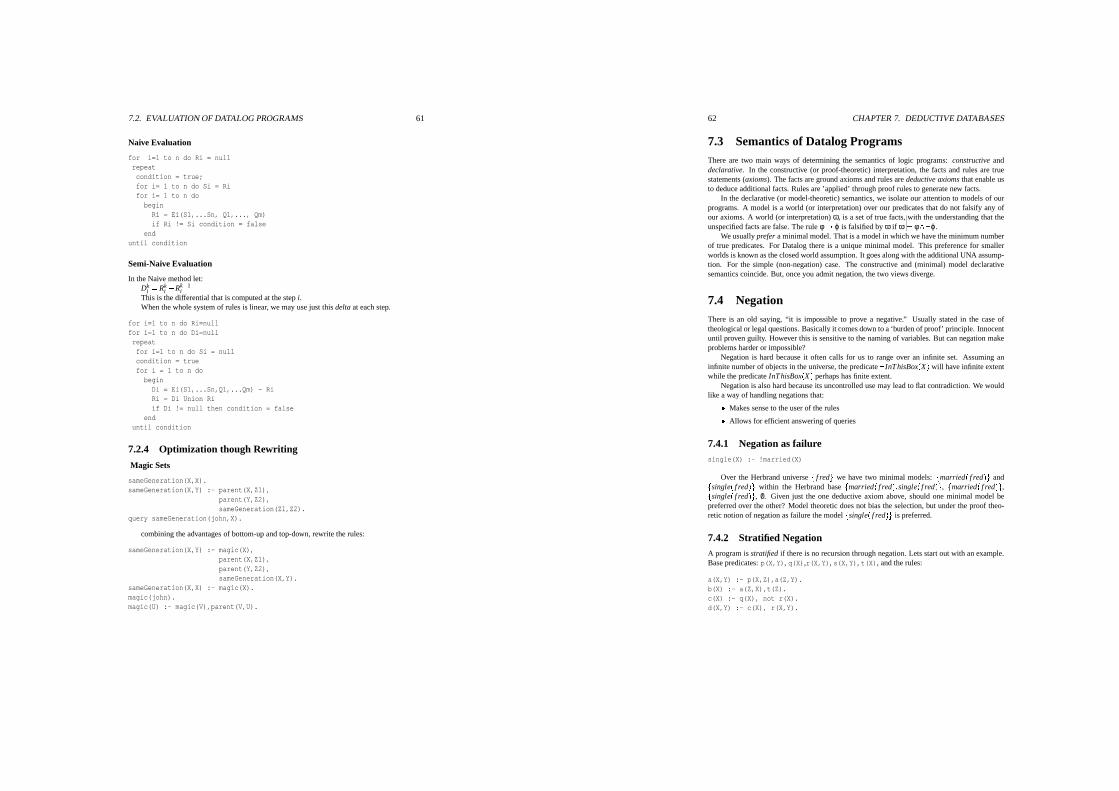
7.2. EVALUATION OF DATALOG PROGRAMS 61
Naive Evaluation
for i=1 to n do Ri = nullrepeatcondition = true;for i= 1 to n do Si = Rifor i= 1 to n dobeginRi = Ei(S1,...Sn, Q1,..., Qm)if Ri != Si condition = false
enduntil condition
Semi-Naive Evaluation
In the Naive method let:Dk
i
� Rki
� Rk � 1i
This is the differential that is computed at the step i.When the whole system of rules is linear, we may use just this delta at each step.
for i=1 to n do Ri=nullfor i=1 to n do Di=nullrepeatfor i=1 to n do Si = nullcondition = truefor i = 1 to n dobeginDi = Ei(S1,...Sn,Q1,...Qm) - RiRi = Di Union Riif Di != null then condition = false
enduntil condition
7.2.4 Optimization though Rewriting
Magic Sets
sameGeneration(X,X).sameGeneration(X,Y) :- parent(X,Z1),
parent(Y,Z2),sameGeneration(Z1,Z2).
query sameGeneration(john,X).
combining the advantages of bottom-up and top-down, rewrite the rules:
sameGeneration(X,Y) :- magic(X),parent(X,Z1),parent(Y,Z2),sameGeneration(X,Y).
sameGeneration(X,X) :- magic(X).magic(john).magic(U) :- magic(V),parent(V,U).
62 CHAPTER 7. DEDUCTIVE DATABASES
7.3 Semantics of Datalog ProgramsThere are two main ways of determining the semantics of logic programs: constructive anddeclarative. In the constructive (or proof-theoretic) interpretation, the facts and rules are truestatements (axioms). The facts are ground axioms and rules are deductive axioms that enable usto deduce additional facts. Rules are ’applied’ through proof rules to generate new facts.
In the declarative (or model-theoretic) semantics, we isolate our attention to models of ourprograms. A model is a world (or interpretation) over our predicates that do not falsify any ofour axioms. A world (or interpretation) ω, is a set of true facts, with the understanding that theunspecified facts are false. The rule φ � ϕ is falsified by ω if ω �
� φ� � ϕ.We usually prefer a minimal model. That is a model in which we have the minimum number
of true predicates. For Datalog there is a unique minimal model. This preference for smallerworlds is known as the closed world assumption. It goes along with the additional UNA assump-tion. For the simple (non-negation) case. The constructive and (minimal) model declarativesemantics coincide. But, once you admit negation, the two views diverge.
7.4 NegationThere is an old saying, “it is impossible to prove a negative.” Usually stated in the case oftheological or legal questions. Basically it comes down to a ‘burden of proof’ principle. Innocentuntil proven guilty. However this is sensitive to the naming of variables. But can negation makeproblems harder or impossible?
Negation is hard because it often calls for us to range over an infinite set. Assuming aninfinite number of objects in the universe, the predicate � InThisBox� X � will have infinite extentwhile the predicate InThisBox� X � perhaps has finite extent.
Negation is also hard because its uncontrolled use may lead to flat contradiction. We wouldlike a way of handling negations that:
� Makes sense to the user of the rules
� Allows for efficient answering of queries
7.4.1 Negation as failuresingle(X) :- !married(X)
Over the Herbrand universe � f red � we have two minimal models: � married� f red � � and
� single� f red � � within the Herbrand base � married� f red � �
single� f red � � , � married� f red � � ,
� single� f red � � , /0. Given just the one deductive axiom above, should one minimal model bepreferred over the other? Model theoretic does not bias the selection, but under the proof theo-retic notion of negation as failure the model � single� f red � � is preferred.
7.4.2 Stratified NegationA program is stratified if there is no recursion through negation. Lets start out with an example.Base predicates: p(X,Y), q(X),r(X,Y), s(X,Y), t(X), and the rules:
a(X,Y) :- p(X,Z),a(Z,Y).b(X) :- a(Z,X),t(Z).c(X) :- q(X), not r(X).d(X,Y) :- c(X), r(X,Y).

7.5. DISJUNCTION 63
d(X,Y) :- c(X), r(X,Z), d(Z,Y).e(X) :- c(X), s(X,Y), not d(X,Y).
We induce the relations � and � over the predicates such that p � q if we have the rule:p � � � �
�
q
�� � � and p � q if we have the rule: p � � � �
�
� q
�� � � . A program P is stratified if there is no
sequence of predicate symbols of P in the form p1θ1 p2� � � θk � 1 pk such that θ � � � �
� � , at leastone θ j �� �� and p1 � pk.
These partitions are called layers and there is a non-reflexive, anti-symmetric, transitiveordering � over these layers. Layers lower in the ordering � propagate their answers to higherlayers. Before we propagate results to a higher layer i we calculate the fixed-points for all groupsj where i � j.
7.4.3 Lists and SetsWe support lists with a special notation.
[] denotes the empty list[X|Y] is a list with the head X and the tail Y.[a,b,c,...] is short for [a|[b|[c...]]]
part(’socks’, [brown, black, blue]).
To create the unnested relation part_color(I,C)
subc(I,L) :- part(I, L).subc(I,T) :- subc(I, [H|T]).part_color(I,C) :- subc(I, [C|_]).
armed(’Natives’, {sticks, stones, spears}).armed(’Pilgrim’,{musket,sword}).armed(’Pirates’,{musket,sword}).
Notice that order is not important.
query armed(X,{sword,musket})
Nor is duplication:
query armed(X,{sword,musket,sword})
Here we show the use of a built in set predicate
has_arms(X,A) :- armed(X,S), member(A,S).query has_arms(X,’musket’)
we also have: subset, union, difference, intersection, and cardinality.
7.5 DisjunctionNote that we shall not adequately handle the notion of representing the plain unbiased disjunc-tion:
drinksSoda(X) or drinksBeer(X)
64 CHAPTER 7. DEDUCTIVE DATABASES
Under declarative (model theoretic) semantics this is captured in the rule:
drinksSoda(X) :- !drinksBeer(X).
Under constructive (proof theoretic) semantics we deduce that someone drinks soda if wefind that they do not drink beer. But we do not achieve the reverse deduction that someone drinksbeer if they are found to not be drinking soda. One solution would be to use two rules to expressthe disjunction. But this violates Stratified Negation.
7.6 Non-monotonicityOne final theoretical point to be made revolves around questions of monotonicity. In classicallogic the set of facts deduced grows monotonically as we learn new facts.
if p � q then p� r � q.Note that we have monotonicity for first order and simple programs. Negation kills these
monotonic properties. The non-monotonic formalism underlying stratified negation is callednegation by failure. It is in essence equivalent to the other first generation non-monotonic for-malisms like simple circumscription [?] and the closed world assumption [?].
7.7 Specializations of the Relational ModelWhile we are in the business of talking about extensions to the relational model, it is importantto highlight some specializations of the model. These specializations of the relational model areuseful for tasks such as query optimization, data integration, answering queries over views, etc.
One of the first specializations to be noted is the case of conjunctive queries. These arethe select-project-join queries of the relational algebra, the conjunctive queries with out nega-tion queries of tuple calculus and the safe datalog queries that are over single EDB and builtinpredicates.
There are algorithms that decide query containment and hence equivalence between thesequeries. There are also algorithms for equivalent rewritings of these queries as well as maximallycontained rewritings of such queries.
7.8 Bibliographical and Historical RemarksLDL stands for Logic Data Language. LDL was initially developed at MCC, Austin, TX. Fromthere LDL++ was thereafter developed at UCLA. LDL++ enables programs in all the levels ofthe following hierarchy2.
Updates, Procedural Extensions, Aggregrate Operations,Choice
First Order − no recursion
Simple − recursion, no negation
Evaluable Predicates, Constraints
Admissible − stratified negation
2Relational Algebra � Tuple Calculus � Domain Calculus � non-recursive + negation as failure.

7.8. BIBLIOGRAPHICAL AND HISTORICAL REMARKS 65
The term extensional and intensional come from the philosophy of language.
66 CHAPTER 7. DEDUCTIVE DATABASES
7.9 Exercises1. Datalog Queries
Consider the following schema:
database({subParts(id:number,subParts:any),description(id:number, desc:String),manufacturedBy(id:number, desc:String)
}).
With an example EDB:
subParts(001, {002,003})subParts(002,{004}).description(001, ’Motor Rocket’)manufacturedBy(001, ’King Weasel Inc.’)description(002, ’Tin Barrel’)manufacturedBy(002, ’King Weasel Inc.’)description(003, ’Duster Motor’)manufacturedBy(003,’Sappy Co.’)description(004, ’Tin Lid’).manufacturedBy(004, ’King Weasel Inc.’)....
a.) define the IDB predicate subPart(Part, SubPart) which flattens the SubPartsrelation.
b.) define the IDB predicate within(Part, SubPart) which is true when SubPart issomewhere within Part.
c.) define the IDB predicate soleyManufacturedBy(Part, Company).
2. Person(Name, Gender, DateOfBirth, DateOfDeath, Country)Parent(ParentName, ChildName)Worked(Name, Company, Title)
Note that for living individuals the date of death is now (kind of scary - ehh?)
a. Define the IDB predicate for Living(Name)
b. Define the IDB predicate Ancestor(X,Y)
c. Define the predicate that returns all living individuals who have worked at McDon-ald’s
d. Define the predicate that returns all living individuals who have never worked atMcDonald’s
e. Define the predicate for individuals who have a Swedish ancestor.
f. Define the predicate for Swedish individuals all of whose ancestors are Swedish.

Chapter 8
Semi-Structured Databases andXML
XML is Lisp’s bastard nephew, with uglier syntax and no semantics. Yet XMLis poised to enable the creation of a web of data that [in relative terms] dwarfsanything since the Library of Alexandria. (Phillip Wadler 2001, VLDB)
8.1 Semi-structured Data
Before we look at XML, let us look at a related notion of semi-structured data. Similar to oldfashioned semantic networks, semi-structured data is a collection of nodes, some leaf and someinternal connected by directed labeled edges. A root node is an internal node with no incomingedges. Edges have labels and leaf nodes have associated atomic data values.
Semi-structured data may be thought of as schemaless. Or, perhaps in a more positive sense,self-describing. It is in fact well suited to information integration tasks. It is also similar tospecific type of stand alone XML usage.
Querying semistructured data may be seen as a regular path querying. Let us adopt * as thekleene star of a set of labels. And let us use + as union of regular expressions. The semantics isclear enough. Given a node, define the function T� V
�
P � � 2P. The set of base path expressionsare defined as e the empty string, σ a simple label and ? a wild-card symbol. If p1 and p2 arepath expressions, then p1 p2, p� 1, p1 � p2 and p1&p2 are path expressions.
8.2 The basic constructs of XML
XML (Extensible Mark-up Language) was started by Tim Berners-Lee and the W3C in 1996 andis a tag-based standard that is a properly within SGML (Standardized General Markup Language)(1986), but more general than HTML (Hyper-Text Mark-up Language). XML is able to representdocument, semi-structured and structured data.
In the structured and document case, XML employs DTDs (Document Type Definitions)that specify constraints on recursively embedded tag-delineated expressions. Thus a DTD maybe viewed as a type of schema over a “tree-like” data model. A set of legal expressions saved ina file is a valid XML document of the DTD type.
67
68 CHAPTER 8. SEMI-STRUCTURED DATABASES AND XML
When XML is used without a DTD we say that it is being used in stand-alone mode. In sucha mode XML documents may be said to be schemaless or self-describing. In such a case, XMLis essentially giving a type of semi-structured data model.
8.2.1 Semi-structured XMLLet us start with the case where XML documents are schemaless. This type of use is indicatedin the document by:
<? XML VERSION = "1.0" STANDALONE = "yes" ?><BODY>...</BODY>
The only condition over such documents is that they are syntactically well-formed. So, as anexample we might just write a self describing document such as:
<? XML VERSION = "1.0" STANDALONE = "yes"?><BODY><FRIEND><NAME> Bob Smith </NAME><PHONE> 313-668-3242 </NAME>
</FRIEND>...
</BODY>
We may in fact have some more complexity in the semi-structured case:
<?xml version="1.0" encoding="ISO-8859-1"?><partlist><part partid="0" name="car"/><part partid="1" partof="0" name="engine"/><part partid="2" partof="0" name="door"/><part partid="3" partof="1" name="piston"/><part partid="4" partof="2" name="window"/><part partid="5" partof="2" name="lock"/><part partid="10" name="skateboard"/><part partid="11" partof="10" name="board"/><part partid="12" partof="10" name="wheel"/><part partid="20" name="canoe"/>
</partlist>
8.2.2 Structuring XML documents through DTDsLet us now consider the case of using XML with the DTD checks turned on. Before we speak ofthe actual documents of content we must define the ’schema’ in the DTD. The gross structure ofa DTD is:
<!DOCTYPE root-tag [<!ELEMENT element-name (components)>...]>

8.2. THE BASIC CONSTRUCTS OF XML 69
Elements define structures that must be blocked off by start and end tags of the elementname. The components specification names a set of sub-elements that are nested within speci-fication of the elements of documents of the DTD type. The special components specification(#PCDATA) specifies that the element is atomic and may have a set of printable characters asits value. The value EMPTY indicates that it is an empty element that consists of just attributes(see below). The ordering of components matters and special symbols indicate the number ofcomponents nested within the element: (0-1) is indicated with a ’?’, (0-X) is indicated with a ’*’,(1-X) is indicated with a ’+’.
Additionally we may wish to add attributes to the elements. Attributes are values that areset in the opening head tag of an element expression. We shall talk a bit more about attributesbelow. For now assume that they are declared in the DTD in a general form as:
<!ATTLIST element-nameattribute-name1 attribute-type1 attribute-default1...attribute-namen attribute-typen attribute-defaultn>
Movie Example DTD
Let us now show an example DTD.
<?xml version="1.0" encoding="ISO-8859-1"?><!DOCTYPE movielist [<!ELEMENT movielist (movie*)><!ELEMENT movie (title, releaseyear, director, cast?, genre+,
country, rating)><!ELEMENT title (#PCDATA)><!ATTLIST title subtitle CDATA #IMPLIED><!ELEMENT releaseyear (#PCDATA)><!ELEMENT director (#PCDATA)><!ELEMENT cast (actor+)><!ELEMENT actor (#PCDATA)><!ATTLIST actor role CDATA #REQUIRED><!ELEMENT genre (#PCDATA)><!ELEMENT country (#PCDATA)><!ELEMENT rating (#PCDATA)><!ATTLIST rating scale CDATA #FIXED "1">
]>
Movie Content File
Now let us continue and show an example document of the MovieList type.
<?xml version="1.0" encoding="ISO-8859-1" standalone="no"?><!DOCTYPE movielist SYSTEM"http://www.cs.umu.se/˜c97fno/movielist.dtd"><movielist><movie><title>2001: A Space Odyssey</title><releaseyear>1968</releaseyear><crew>
70 CHAPTER 8. SEMI-STRUCTURED DATABASES AND XML
<director>Stanley Kubrick</director><writer>Arthur C. Clarke</writer><producer>Stanley Kubrick</producer></crew><cast><character><actor gender="male">Keir Dullea</actor><role>David Bowman</role></character><character><actor gender="male">Douglas Rain</actor><role>HAL 9000</role></character></cast><genre>Sci-Fi</genre><country>UK</country><rating>8.1</rating></movie>...</movielist>
8.2.3 Attribute Data TypesLet us now return to the topic of attributes that modify elements. We recall that attributes aredefined in lists associated with an element.
<!ATTLIST element-nameattribute-name1 attribute-type1 attribute-default1...attribute-namen attribute-typen attribute-defaultn>
The basic types in XML DTDs are:
� ID. Unique ID only allowed once in the document.
� IDREF. Refers to elements with the given ID.
� IDREFS. The same as IDREF, but more than one ID is used.
� ENTITY. Declares the name of an entity.
� ENTITIES. Declares two or more entity names.
� NMTOKEN. Declares a name token. Is any mixture of name characters.
� NMTOKENS. The same as NMTOKEN but more than one name token is declared.
� ENUMERATION. Enumerated attributes can take one of a list of values declared.
� NOTATION. Declares the name of a notation.
� CDATA. String value.
Additionally the default modifiers are:
� #REQUIRED. The attribute must have a value.

8.3. XQUERY 1.0 + XPATH 2.0 71
� #IMPLIED. The attribute is optional.� #FIXED. The attribute has a value that is defined in the DTD.
8.2.4 XSchemaXSchema, uses name spaces, to enable the definition of abstract xsd:element, xsd:sequence,xsd:complexType xsd:unique, xsd:key, xsd:keyref constructs to give a much tighterdatabase like schema document type definition.
The validity check on database files of an XMLSchema document type undergo more ex-pensive integrity checks. Otherwise they are treated just like any other XML document.
8.3 XQuery 1.0 + Xpath 2.0XPath is a simple language to obtain elements from XML documents and XQuery is a fullerquery language that uses XPath as a sub-language.
8.3.1 XPath 2.0XPath specifies expressions that return elements within documents.
Several examples are: /movie/actor which returns all the actor el-ements within movie elements of a document. Thus the command/verb+doc(www.cs.umu.se/ mjm/movielist2.xml)/movie/actor+ achieves this. If one wished tofind any actor in the document at any level, then the XPath expression: //actor should be used.This option is especially useful with stand alone XML documents. Finally there are simplepredicates one may include in XPath queries. And example would be to get all of the maleactors. //actor [gender eq ’male’]. Note that these predicates may also appear along thepath to the elements. Thus /movied [year gt 1970]/actor returns the actors in films after1970.
8.3.2 XQuery 1.0More complex queries specified in so called FLWR (flower) expressions.
FOR <variable bound to individual nodes> INLET <variable bindings to collections of nodes>WHERE <qualifier conditions>RETURN <query result specification>
Several examples follow:
<bib>{for $b in $bib/bib//bookwhere ($b/publisher = "Addison-Wesley" and $b/@year > 1991)order by $b/title ascending empty greatestreturn <book>{$b/@year}{$b/title}</book>
}</bib>
72 CHAPTER 8. SEMI-STRUCTURED DATABASES AND XML
<bib><book year="1992"><title>Advanced Programming in the Unix environment</title>
</book><book year="1994"><title>TCP/IP Illustrated</title></book>
</bib>
<parttree>{for $p in $partlist//part[empty(@partof)] return one_level($p)}
</parttree>
<parttree><part partid="0" name="car"><part partid="1" name="engine"><part partid="3" name="piston"/></part><part partid="2" name="door">
<part partid="4" name="window"/><part partid="5" name="lock"/>
</part></part><part partid="10" name="skateboard"><part partid="11" name="board"/><part partid="12" name="wheel"/>
</part><part partid="20" name="canoe"/>
</parttree>
8.4 XML Meta StandardsThe whole W3C effort has been mired in an alphabet soup of (competing) standards. It lookspretty hopeless, but they are trying now to fuse the whole heap together.
� XSL, XSLT - more advanced style sheet language
� XLink - add hyperlinks to other XML documents.
� Xpointer - add links within an XML document
� CSS - style sheet language
� DOM - Document object model. Standard API to manipulating and XML document fromwithin a programming language
� XHTML - the new HTML in XML. Slight changes to HTML.
� RDF - Resource Description Framework
8.5 XML - DTD types
� Meat and Poultry XML (mpXML).
� MathML
� SOAP

8.5. XML - DTD TYPES 73
� VXML� UPnP
� SyncML
� Chemical Markup Language (CML)
� Bioinformatic Sequence Markup Language (BSML)
� ...
XML promises structured data on the web.
74 CHAPTER 8. SEMI-STRUCTURED DATABASES AND XML
8.6 Exercises1. XML DTDs
Consider the following schema:
SubParts(Part#, subParts)Description(Part#, Description)ManufacturedBy(Part#, Company)
With an example EDB:
SubParts(001, {002,003})Description(001, ’Motor Rocket’)ManufacturedBy(001, ’King Weasel Inc.’)Description(002, ’Tin Barrel’)ManufacturedBy(002, ’King Weasel Inc.’)Description(003, ’Duster Motor’)ManufacturedBy(003,’Sappy Co.’)...
a.) Define a DTD corresponding to the schema in problem 3.
b.) Create a document of this DTD type that captures the database state depicted inproblem 3.

Chapter 9
Managing Uncertainty inDatabases
Ignoring intrinsic uncertainty at the quantum level, we may assume that the world itself is certainand that uncertainty in databases arises from the database’s imperfect belief about the world.For this we use the term data uncertainty. Thus we shall always talk about data uncertaintywith respect to a given schema that captures relevant aspect of the world at some level of detail.Furthermore we stipulate that, in principle, we could have certain information over the givenschema. As an example, it seems reasonable to suppose that we could have certain informationover the schema:
Student (Number, FirstName, LastName, Height, Age, Gender, Major)
The reasons for data uncertainty are numerous.
� Unreliable Information Sources - faulty reading instrument, input forms filled out incor-rectly (intentionally or inadvertently)
� System Errors - transmission noise, delays in processing updates, system failures, cor-rupted data (failure or sabotage)
� Information Gathering - Process forces estimation or judgment
� Data Volume - too much to capture, must approximate
� Heterogeneous Database EnvironmentsCompleteness and consistency are not maintained between separate systems. Thus if weattempt to fuse two systems together there will be clashes resulting in uncertainties.
The problem of data uncertainty is orthogonal to the problem of query uncertainty. In queryuncertainty we may use approximate or vague terms which would introduce uncertainty over theway in which the system interprets and processes user queries. Thus even if we did have certaindata for the above schema, how would we answer the query “give the tall science students.”What is ’tall’?, what is a ’science’ student?
9.1 Managing Data UncertaintyThe strongest form of uncertainty is simply missing information, the case of being unable tosay whether a fact is true or not or an attribute value is such and such within a tuple. This is a
75
76 CHAPTER 9. MANAGING UNCERTAINTY IN DATABASES
result of the database being incomplete and thus missing any information pertaining to the factin question.
Another form of uncertainty is imprecision. In such a case the system lacks specificity, buthas some relevant information. Thus the system may record its belief that “John is between 21and 24 years old”. Often such data is said to be disjunctive when there is a set of possible valuesfor the data value, one of which must be true. If we tag each data value within the disjunct witha bit of probability density, such that all values across the disjunction sum to 1, then data is saidto be probabilistic.
Finally there is the notion of using vague terms to state belief over the domain of thedatabase. So, for example, we may assert that “John is a young adult”. When language is con-cerned, there is another problem of ambiguity. Ambiguity arises when there are several possibleinterpretations of a given symbol. For example ‘salary’ may mean yearly or nine month.
For relational systems, data uncertainty may be over attribute values (e.g. “when is JohnSmith’s major?”), tuple values (e.g. “is there a student names ’John Smith’?”).
9.1.1 Incompleteness
Null Values
The traditional method to signal incompleteness over attribute values is through the value NULL.Of course NULL usually means either: unavailability, non-existence or inapplicability.
Thus if we come across the student tuple:
Student (001, ’John’, ’Smith’, 170, 23, NULL)
This may mean that we do not know Smith’s major (unavailability), Smith does not have amajor (non-existence) or Smith is the type of student for which the major attribute is meaning-less1(inapplicability). Naturally the first notion is the one that applies to NULL values in thecontext of data uncertainty. A problem that comes up with respect to NULL values conceivedthis way, is how to interpret queries over databases with such NULL values.
Incompleteness Descriptions
NULL values are a way to represent incompleteness at the level of attribute values, but howare we able to handle the cases of incompleteness with respect to whole tuples? Often one isprepared to make very specific declarations of soundness and completeness in a database. Forexample one may be willing to say that a database has all the records for all of the students inTDBD15. In any case these declarations of local soundness and completeness are fine-grainedviews2 and are asserted as a dynamic part of populating or modifying the database.
The problem is that these declarations should be merged and managed so that when thedatabase is queried, a coherent description of the databases completeness (or incompleteness)may be provided with respect to the specific query. Thus when the user asks for all the studentsin TDBD15 and TDBC76, the user should be informed that their answer is complete for TDBD15and not so for TDBC76.
More abstractly, consider that we have a set of n views: � � �� � �
�
� � that describe the portion ofthe schema for which the database has complete coverage. The problem is, given a query � , cal-
1Smith may be a non-degree or visiting student2We shall assume that such views are sound. The notion of complete in this case corresponds to the
closed world assumption being applicable over the view.

9.1. MANAGING DATA UNCERTAINTY 77
culate the portion of � that may be answered with certainty3 using the views. The answer to thisproblem is a disjoint partition of the original query � into two queries �� � �� �� � and � � �� � �� � � �
where �� � �� �� � is the portion of the query that may be answered with certainty and � � �� � �� � � �
is the remainder that may not be answered with certainty over the views.
9.1.2 Imprecision
Disjunctive
Disjunctive databases are ones in which domain values may be represented as disjunctive sets.One may also include the capability of range constraints and negative information.
Probability
Probability is the classical approach to uncertainty. It can be viewed as an extension to thedisjunctive case where every bit of data gets some probability density, that, across all cases,sums to 1.
The easiest case for probabilistic databases is the case where each tuple represents an inter-pretation or possible world. Each tuple has a real variable that records the amount of probabilitydensity associated with the case represented by the tuple. In this way a full joint probabilitydistribution is represented in the relation.
Note that simple Bayesian network models give a structured way to generate such a distribu-tions. Note also that aggregation queries may be used to obtain answers to conditional queries.Thus we may answer arbitrary queries through P� A � B � � P� AB � � P� B � .
The probability case in the attribute value case is not as straight forward.
9.1.3 Vagueness
Often we wish to encode values in a database using descriptive terms. The general method to dothis at the representation level is through fuzzy sets.
Fuzzy Sets
A fuzzy sets are defined through ’graded membership’ functions over the actual domain of thevalue. We consider the piecewise linear case. In such a case there are well founded definitionsof complement, intersection, union, etc.
3The notion of certain answers here is that of certain answers in [1] under closed-world views. Specifi-cally an answer τ to query � is certain, if it is an answer to � over all complete databases where � � � � � � arecomplete views.
78 CHAPTER 9. MANAGING UNCERTAINTY IN DATABASES
1.0
0.5
YOUNG-ADULT
Age
Membership
10 20 30 40 50
In databases we may represent each tuple as being assigned a grade of membership in therelation
Fluent(Person, Language)
Fluent(’Mike M.’, ’English’): 1.0Fluent(’Mike M.’, ’Swedish’): 0.40Fluent(’Mike M.’, ’French’): 0.01
In another option, attribute values are given fuzzy category names.
People(Name,Age)
People(’Freddy’, ’YoungAdult’)People(’Jim’, ’Child’)
We may use both options simultaneously. The first option is easier to implement over stan-dard databases. The second notion requires the definition of fuzzy comparison operators (e.g.roughly-equal-to, much-larger-than, etc).
9.2 Managing Query Uncertainty
The basic types of query uncertainty stem from vague terms being used in the query, queriescalling for similar or near answers. Without loss of generality, we shall assume that the databaseover which we queries are applied is certain.
9.2.1 Vagueness
The techniques described for fuzzy sets may be applied for answering vague queries. In fact,it can be argued, that such notions of vagueness are best isolated to the language level, sittingabove belief.
9.3. BIBLIOGRAPHICAL AND HISTORICAL REMARKS 79
9.2.2 SimilaritySQL comes built in with one similarity type functionality. This is the LIKE operator.
A very common approach to similarity is to develop a distance function over the set tuplesbeing queried for. One may then of course issue similarity based queries. Give students similarto ’John Smith’. This type of querying is not so common in databases, but is the normal casein information retrieval. In such a case one looks for documents that are similar to those usingsuch and such keywords. The notions of precision (the proportion of relevant material withinthe answer set) and recall (the proportion of all relevant material obtained) are used to assess thequality of such information retrieval systems. Prototype systems have done the same for queryby image content, etc.
9.3 Bibliographical and Historical Remarks
9.4 Exercises
80 CHAPTER 9. MANAGING UNCERTAINTY IN DATABASES

Chapter 10
Data Mining
’Data mining’ is like saying ’dirt mining’, but the name stuck. Loosely speaking data miningis, ”the generation of useful knowledge from data”. Most data mining techniques originated instatistics and machine learning. KDD (Knowledge Discovery in Databases) is an overall processof which Data Mining is a component. KDD involves selection, preprocessing, translation, datamining, interpretation, evaluation and presentation.
In this book data is in relational form1. Knowledge is in the form of ‘rules’. One type ofrule is a classification rule which is used to judge tuples into or out of a target concept. A relatednotion is that of clustering tuples or attribute values into a number of classes. Additionally rulesmay also be express causal or evidence relationships within the domain. However, since it isdifficult to establish such knowledge from data alone, we usually settle for the weaker notion ofgenerating association rules.
We shall cover the basic techniques to induce classification, clustering and association rulesfrom relational data. Most techniques designed to do this are single relation techniques. We shallend this chapter with some comments about multi-table data-mining techniques and challenges.
10.1 Induction of Classification RulesWe are given a relational table with attributes. Of these attributes there exist a class attribute forwhich we would like to classify tuples, based on a set of relevant attributes.
Thus given data in the table:
Risk(personId, age, carType, gender, risk)001 33 Family M Low002 21 Sports M High...
We may induce the following classification rule which predicts insurance risk over a table ofpersonal information.
HighRisk(ID) :- PersonalInfo(ID, AGE, CARTYPE, GENDER),AGE > 16, AGE < 25, GENDER = ’Male’, CARTYPE = ’Sports’.
In this induction task, risk is the class variable and age, carType and carType are therelevant attributes.
1Note that this may include collection type attributes.
81
82 CHAPTER 10. DATA MINING
10.1.1 Decision Trees
The classical method to obtain classification rules is to induce a decision trees. A decision treefor the example above could be:
Age
Car Type
Gender
<25 >=25
Sport Sedan
Male Female
NO
NO
NOYES
Each internal node specifies a single relevant attribute. Each outgoing edge on an internalnode has a predicate involving the relevant attribute so that one and only one edge will apply toa given tuple. Each leaf is labeled with a value of the class attribute. Every path from root to leafdetermines a classification rule. Decision trees are well behaved because classification is fast,usually involving only a few simple questions, and the structure of the tree is easy to interpret.Additionally it is straight forward to translate decision trees into a set of classification rules.
Decision trees are usually built in a top-down, greedy manner. The core algorithm must pickfrom a set of possible splits. A split is a partition of the relevant training examples based on aset of conditions over an attribute. Normally splits that exhibit the highest information gain arethose that are picked. The resulting partition of the database into n subtables, are the inputs toa recursive call to the splitting algorithm. Splitting ceases once the best possible informationgain falls below a certain threshold. See 5, derived from the academic tool C4.5 is the leadingdecision tree induction tool.
10.2 Clustering Values and Tuples
Clustering is an unsupervised learning method where the input is a table of tuples with a set ofrelevant attributes marked. The output is a set of n cluster (or class) definitions which ‘nicely’partition the space of tuples. In general the tuples that lie in the same cluster should be similar,and tuples within distinct clusters should be dissimilar.
Clustering is often used as a preprocessing step for classification, especially with respect todiscretization of continuous attribute values. However it should be noted that clustering may beused as a tool in itself to identify natural groupings of the tuples. Finally it can also be used foroutliers detection.
So what constitutes a natural grouping, and how is it measured? The most often used mea-sure is distance. We of course want the distance between samples belonging to the same clusterto be less than the distance between samples in different clusters. When distance is used asmeasure, a metric is needed. A general form of is the Minkowski metric:
d � x � x �� �
�
d
∑k� 1
� xk� x �
k�
q
1 q

10.3. MINING FOR ASSOCIATION RULES 83
When q � 2 it is more known as Euclidean metric. Setting q � 1 gives the Manhattan or‘city block’ distance.
An example of a clustering algorithm is the k-means algorithm. It is given in 10.1. Thecomplexity of the algorithm is O� ndcT � , where n is the number of samples (tuples), d is thenumber of features (columns in the tuples), c is the number of clusters. T is the number ofiterations, in practice T will be much less than n.
Input n, number of clusters.Samples - Unlabeled data samples.
Output Cluster center.
1: Initialize all cluster-center µi to e.g. a random sample.2: repeat3: for all samples do4: Classify the sample according to nearest µ.5: end for6: for all µi do7: Recompute µi as the mean value of the samples belonging to that cluster.8: end for9: until No change in µ1 � µ2 �� � � � µn.
10: return µ1 � µ2 �� � � � µn.
Figure 10.1: k-means clustering
So how do we assess the result of a clustering algorithm. The simplest and most widely usedcriterion function for clustering is the sum-of-squared-error function.
Je �
c
∑i � 1
∑x � Di
� x � mi� 2�
The k-means algorithm is an example of an iterative optimization technique. Like all otheralgorithms in this category it is only guaranteed to find a locally optimal solution, but not theglobal optimum. A major drawback of the k-means algorithm is the need to specify the numberof clusters. A direct approach is to execute the algorithm for increasing values of k. By observingthe behavior of the error criterion a good value of k can often be determined if the data is wellbehaved. It is then expected that the error decreases rapidly until the optimal value, where afterit decreases much more slowly until the number of clusters equals the number of data points.
10.3 Mining for Association RulesOne of the most well known techniques in data mining is the mining of association rules. Sup-pose we have the following transaction database.
Transaction Basket-------------------------1 {milk, bread, juice}2 {milk, juice}
84 CHAPTER 10. DATA MINING
3 {milk, eggs}4 {bread, cookies, coffee}
An association rule is: X � Y where X at Y are sets of items and X � Y � /0. For example
� milk � � � juice � . “67% of those who buy milk also buy juice”.
10.3.1 Support and Confidence
There are two important measures associated with a rule, the rule’s support and the rule’s confi-dence. A rule’s support is the percentage of transactions where the association rule is verified2.A rule’s confidence is the proportion of transaction that verify the rule, to those that either falsify3 or verify the rule. Thus in the example above � milk � � � juice � has 50% support and 67%confidence. � bread � � � juice � has 25% support and 50% confidence.4 Note that the followingproperties hold for support.
1. if support� X � � β then support� Y � � β where Y � X .
2. if support� X � � β then support� X � Y � � β.
These properties will be exploited in algorithms that search out association rules over item sets.Support and confidence are the most commonly used measures of the importance of a rule.
There are also other useful measures, for example lift. Assume the following probabilities fortwo items X and Y in market basket data: P� X � � 0� 6
�
P� Y � � 0� 75
�
P� X � Y � � 0� 4 and thefollowing rule is then discovered: X � Y [support = 40%, confidence = 66%]. This rule can bemislead the user to believe that a purchase of X implies a purchase of Y . In fact X and Y arenegatively correlated, and thus a purchase of one of them decreases the likelihood of purchasing
the other. Correlation is measured by corrX � Y � P � X � Y �
P � X � P � Y �� P� Y � X � � P� Y � , also called the lift
of the rule X � Y . If this value is less than 1� 0 the occurrence of X is negatively correlatedwith the occurrence of Y . A value greater than 1� 0 means that the occurrence of X suggests theoccurrence of Y . If the lift equals 1� 0, then X and Y are independent.
10.3.2 The Naive Algorithm for Mining Association Rules
Over a set of m distinct objects there are O� 2 � 2m
� syntactically correct associations. (Thisbound is loose because X and Y are disjoint.) We wish to only report interesting rules - thoseover a confidence threshold α and over a support threshold β.
1. Compute all sets5 with sufficient ( � β) support.
2. Among each large item set X , consider the rules X � Y � Y where Y � X :
If support � X �
support � Y �� α then add X � Y � Y to the answer set 6.
Still we have all O� 2m
� large item sets to consider. Let us keep this algorithm, but considera more efficient method to compute the large itemsets..
2Both the antecedent and consequent sets are within the transaction3The antecedent set, but not the consequent set is in the transaction4Given that P � A � B
P � A � B
P � B , we may interpret the association rule X � Y as P � Y � S � X � S
P � X � Y � S
P � X � S
where S are the set of items in the transaction. Seen this way, P � X � Y � S is the “support” and P � Y � S
� X � S is the “confidence’.5Termed the“large item sets”6By property 1 such a rule will have proper support.

10.3. MINING FOR ASSOCIATION RULES 85
10.3.3 The Apriori Algorithm
By exploiting property 2 we can improve the naive algorithm:
1. Test support for item sets of size 1 and discard those with support less than β.
2. Generate all distinct pairwise combinations of 1-item sets (generating the 2-item sets).Discard those with support less than β.
3. Generate the k-th itemset by self joining the k � 1-th itemsets k � 1. Discard any sets withinsufficient support.
4. Repeat until no additional items sets have sufficient support.
This generates all of the large item sets. Requires k scans of the database. In addition wemay store pre-computed large item-set supports for quick confidence calculations.
The key observation is that any subset of a large itemset is also large. The first step whengenerating the large k-itemsets is to join itemsets with k � 1 items. These itemsets are calledpotentially large itemsets. The second step then, is to delete all itemsets from the potentiallylarge itemsets, that have a subset that is not large. As an example[?], let L3 �
� � 1
�
2
�
3 � � � 1
�
2
�
4 � �
� 1
�
3
�
4 � � � 1
�
3
�
5 � � � 2
�
3
�
4 � � . After step 3, C4 �� � 1
�
2
�
3
�
4 � � � 1�
3�
4
�
5 � � . The itemset � 1
�
4
�
5 �
is not in L3, it will therefore be pruned from C4 in step 5. The algorithm concludes a priorithat the only possible large itemset of size 4 is � 1
�
2
�
3
�
4 � without considering the transactions inthe database, thus the name ’a priori’. The Apriori algorithm scales linearly with the number oftransactions[?].
10.3.4 Association Rules among Hierarchies
We may obtain more general association rules if we group items into categories. But we shouldobviously exclude the intra-hierarchy associations (e.g. � crest � � � toothpaste � ). In contrast,the inter-hierarchy associations may be interesting � Du f f � Beer � � � Pain � Killers � .
The problem with hierarchies is that it is hard to find strong associations among items at deeplevels. On the other hand, rules discovered at the top levels of the hierarchies are more likely tojust represent common sense knowledge [?]. The way to mine rules across hierarchies is usuallyto start at the topmost level and move down. A problem is that items at deeper levels will occurless frequently, so it might be a good idea to have lower support thresholds at deeper levels. Thiscomplicates the search procedure however, because the child of a node that is ‘infrequent’ canbe ‘frequent’ if the threshold for the child level is lower than at the parent level.
10.3.5 Negative Associations
Consider the association rule, “85% of people who buy yogurt do not buy soda”. In general itis very hard not to get swamped with meaningless rules. For example the rule “100% of peoplewho buy toothpicks do not buy Trocadero.”
Using prior knowledge in the form of hierarchies can help determine what is an interestingrule. “40% of people who by cigarettes buy beer, but 10% of people who buy Camels, do notbuy Pripps”. You need access to the distribution of market share among beer and cigarettes todetermine if this is unexpected, and hence interesting. What about using the sample itself topredict market share. Would this work?
86 CHAPTER 10. DATA MINING
10.4 Towards Multi-Relation Data-mining
10.4.1 Multi relationalBecause performance is a high priority, data-mining has initially been applied over single tables.This works well because, a large body of prior work is available for the single table case (e.g. atuple may be seen as a feature vector[?]). Single relation approaches can often be successfullyextended to handle multi-relational databases. To upgrade an algorithm to the multi-relationcase, it is usually necessary to upgrade the key concepts. For example, to upgrade a clusteringalgorithm, it is necessary to define the notion of distance between tuples in the multi-relationcase. Once this is done, the rest of the algorithm can often be used more or less intact. It is oftenthe case that the multi relational algorithm has the propositional algorithm as a special case.
Moving up to a multi relational algorithm can have several advantages.
� There is no longer the need to translate the data, by joining and aggregation, so that thedata fits in a single table. Instead multi relational methods can be applied directly.
� Translation to a single table can cause loss of information.
� Translation may result in a table that is to large to handle.
10.5 Bibliographical and Historical RemarksThe most well known algorithm in the data mining field is the Apriori algorithm for findingassociation rules. It was developed by the Quest team at IBM. The first formulation of theproblem of finding association rules appears in Agrawal, Imielinski and Swami 93 [?].
From that research has then sprung a large number of research papers and patents. IBMcurrently holds around 40 patents related to data mining.
From the start, one of the major aims of the research have been to make mining of very large,real life databases practical. Very large can nowadays mean a Terra-byte or more. Traditionallymany algorithms in statistical methods and machine learning have made the assumption that alldata will fit in main memory. Therefore much effort has gone into handling larger databases [?].
10.6 Exercises

Bibliography
[1] S. Abiteboul and O. Duschka. Complexity of answering queries using materialized views.In Sym. on Principles of Database Systems, pages 254–263, 1998.
[2] E. Codd. Relational completeness of data base sublanguages. In R. Rustin, editor, DatabaseSystems, pages 33–64. Prentice-Hall, 1972.
[3] R. Elmasri and S. Navathe. Fundamentals of Database Systems 3rd edition. Addison Wesley,2000.
87