Scholars' Mine Scholars' Mine

Masters Theses Student Theses and Dissertations

1967

Relationships among the metallurgical condition, hardness, and Relationships among the metallurgical condition, hardness, and

the electrical conductivity of aluminum alloys the electrical conductivity of aluminum alloys

Richard A. Mueller

Follow this and additional works at: https://scholarsmine.mst.edu/masters_theses

Part of the Metallurgy Commons

Department: Department:

Recommended Citation Recommended Citation Mueller, Richard A., "Relationships among the metallurgical condition, hardness, and the electrical conductivity of aluminum alloys" (1967). Masters Theses. 6808. https://scholarsmine.mst.edu/masters_theses/6808

This thesis is brought to you by Scholars' Mine, a service of the Missouri S&T Library and Learning Resources. This work is protected by U. S. Copyright Law. Unauthorized use including reproduction for redistribution requires the permission of the copyright holder. For more information, please contact scholarsmine@mst.edu.

RELATIONSHIPS AMONG THE METALLURGICAL CONDITION,

HARDNESS t AND THE ELECTRICAL CONDUCTIVITY

OF AWMINUM ALIIJYS

BY

RICHARD A. MUELLER - / 1.3 f' -

A

THESIS

submitted to the faculty of

THE UNIVERSITY OF MISSOURI AT ROLLA

in partial fulfuUme:nt of the requirements for the

Degree of

MASTER OF SCIENCE IN METALLURGICAL ENGINEERING

ROLLA, MISSOURI

Approved by

~ M ~ (advisor) j)P?1d~i~ /. 4~ iliWlA

11

ABSTRACT

Electrical conductivity measurements (eddy current determined)

combined with indentation hardness measurements are now being used

throughout the aerospace 1ndustry for nondestruotive evaluation of the

metallurgical condition of commercial precipitation hardenable alumi­

num alloys. The review of literature and experiments with two alumi­

num alloys, 7178 and a 5% Zn-Al binary, have shown that skilled

interpretation of hardness-conductivity data depends not only upon a

qualitative understanding of the modern wave mechanical theories of

electron conduction, but also upon some knowledge of the precipitation

reaction kinetics. In particular, the effects of "quenched-in" vacan­

cies and retrogression upon the reaction kinetics must be considered.

Studies of conduotivity vs temperature in the range of 0 to 7 SOF.

show that the resulting conductivity changes do not result in increased

interpretative information and that Matthiessen's rule and Hansen's

equation both apply. Hansen's equation relates conductivity (K) of a

sample to its.temperature coeffioient .of resistance (ot.) in the form of

K = B~+ C where Band C are constants. The values of Band C depend

only upon the alloy system being considered. A practical result is

that the conductivity for an unknown sample can be evaluated at any

known ambient temperature and then corrected to its room temperature

value by calculating the sample's coefficient of resistance using

Hansen's equation. The inverse calculation could also be made.

Key words: Conductivity (Eddy Current); Resistivity: Non­

destructive Testing, AluminUm Alloys.

iii

PREFACE

In recent years, eddy current determined electrical conductivity

measurements have become an invaluable tool for nondestructive testing

commercial precipitation hardenable aluminum alloys for their heat

treat temper. Most of the related available literature contains

essentially empirical data. This thesis is, in part, a qualitative

study of the theoretical aspects of conductivity testing. The exten­

sive review of literature provides the reader with a qualitative under­

standing of the theory which underlies the empirical conductivity data.

The experimental portion of the thesis attempts to utilize the

theory to obtain more interpretive information through conductivity

testing techniques. The work was only partially successful in this

regard; however. a very useful concept was developed which removes the

present limitation of having to conductivity test only in the vicinity

of room temperature.

It is earnestly felt that conductivity testing will, eventually,

rank with indentation hardness testing as a nondestructive test

technique and that this work has contributed to that goal.

The author would like to thank and acknowledge the following:

Dr. A. deS. Brasunas,for his constructive criticism during the prepara­

tion of this thesis; Kaiser Aluminum Corporation, for their preparation

of the high purity binary alloy used in this work; and the McDonnell

Company, for the use of their equipment and facilities.

iv

TABLE OF CONTENTS

Page

LIST OF ILLUSTRATIONS • • • • • • • • • • • • • • • • • • • • •• v LIST OF TABLES • • • • • • • • • • • • • • • • • • • • • . • • •• vii

I.

II.

INTRODUCTION • • . . . . . . . . . . A. B.

Statement of Problem • • . . . . . . . . . . Reasons for Selection •••••••••••••••••

REVIEW OF LITERATURE • • • • . . .. . . .. . ..

A. > Practical Applications • •• B. The Electrical Conductivity of Alloys • •

1. m:p,i.rical"Nlea.. ..... . • . . • . 2. . M04e~n" theGl'y • •• • .. • • •• • • •

3. Factors affecting the conductivity of a.Alloying or impurity elements •• b. Lattice defect.s • • • • •• ;, ••

. . . . . .. , .. . . .

.. .. .. .. . ...

.. .. .. .. . . .. an alloy •• .. .. .. .. .. .... . .. .. .. . ...

o • .. Orderin'g • .. .. . ~ : • .. .. • .. .. • .. .. .. • • , ' .. , d. Temperature effects • • • • • • •• • •

Sp'ecial: Metallurgical Faotors • • • • • • • • • •• L VaCa.ncy effects • • • • • • • • 2. Retrogression effects • • • • • • • • .. . .. .. ..

1

1 2

4

4 11 11 14 15 15 16 16 19 26 26 28

III. DISCUSSrON. · ... • • • • • • • • • • • • • • • • • • •• 32

A. General Aspects • • • • • • • • • • • • • • • • • • •• 32 :8. Basic PTocedures and Eql1iplllsnt • • • • • • • • • • •• 34 c. 71ty3 Heat Treatments.. • ' . • • • • • .. • • • • • • •• )8 D. · dP/dT Studies • • • • • • • • • • • • ..• • • • • • • •• 45 E. · 5f, Zn-Al Heat Treatments • • • • • • • • • • • • • •• 55

IV. CONCLUSIONS.. • • • • • • • • • • • • • • • • • • • • •• . 57

BIBLIOGRAPHY • . . . APPENDIX • . . VITA •••• . .

. . . . .. .. . .. . .. , .. .. .. . . .. . .. .

. . .. .. .. • . • .. 9

60

6)

84

LIST OF ILLUSTRATIONS ILWSTRATIONS

1. CONDUCTIVITY METERS • • • • . . . 2. dP/dT APPARATUS

FIGURES .

. . . .

1. HARDNESS VS CONDUCTIVITY FOR CERTAIN COMMERCIAL A.WMINUM ALLOYS • • • • • • • • • • • • • • • •

2. HARDNESS VS CONDUCTIVITY, SCHEMATIC QUENCH DELAY CURVES FOR ALCLAD 7178 ALUMINUM ALIJJY • • • • •

. . . .

. . . . ..

. . . . .. :3. RESISTANCE VS DEGREE OF SHORT RANGE ORDER • . . . . . . . . . 4. HARDNESS VS CONDUCTIVITY FOR 7178 ALLOY

ROOM TEMPERATURE AGE (75°F.) •••••••

5. HARDNESS VS CONDUCTIVITY FOR 7178 ALIDY. COMPOSITE OF FIGS. 4, 6, 9, 10, 11 AND 12 PLUS ONE SAMPLE AGED AT 1500F. • ••••

6. HARDNESS VS CONDUCTIVITY FOR 7178 ALLOY

. . . . . . . .

. . . . . . . .. AGED AT 450 0 • • • • .. • • • • • • • • . ' • • • . . . . . .

7. RESISTIVITY VS TEMPERATURE FOR TYPICAL SAMPLES. THE 5~ ZINC-AWMINUM ALLOY CURVE IS AN AVERAGE CURVE FOR ALL SAMPLES OF THE ALLOY ••••

8. CONDUCTIVITY VS TEMPERATURE COEFFICIENT OF RESISTANCE FOR TYPICAL SAMPLES. LINE WAS CONSTRUCTED THROUGH USE OF THE METHOD OF LEAST SQUARES ANALYSIS • • • • • • • • • • . . .

. . . . .

. . . FIGURES (CONTAINED IN APPENDIX) • • • • • • • • • . . . . . . 9. HARDNESS VS CONDUCTIVITY FOR 7178 ALLOY

AGED AT 400°F. · · • · · · · · • · • · · · • · · · • · · . 10. HARDNESS VS CONDUCTIVITY FOR 7178 ALLOY

AGED AT 350°F. · · • · · • · · · · · · · · • · · · · • · . 11. HARDNESS VS CONDUCTIVITY FOR 7178 ALLOY

AGED AT 300°F. · · · · · · · • · · · · · · · · · • · · · . 12. HARDNESS VS CONDUCTIVITY FOR 7178 ALLOY

AGED AT 250°F. · · · · • · · · · · · · · · · · • · · · · .

v

Page

36

47

9

22

39

40

43

50

53

6)

64-

65

66

67

vi

LIST OF ILLUSTRATIONS Page

13. CONDUCTIVITY VS TEMPERATURE FOR SAMPLES INDICATED . · · · · • · · · · · · · · • · · · · · · · · · 68

14. CONDUCTIVITY VS TEMPERATURE FOR SAMPLES INDICATED • · · · · · · · · · · · · · · · · • · · · • · · 69

15. CONDUCTIVITY VS TEMPERATURE FOR SAMPLES INDICATED. · · · · · · · · • · · · · · · · · · · · · · · 70

LIST OF TABLES

ALL TABLES ARE CONTAINED IN APPENDIX

TABLES

. . . . . . . . . . . . . .

I AGING TIME, CONDUCTIVITY & HARDNESS FOR DIRECT AGED SAMPLES • . • • • • • • • . . . . . . . .

II AGING T~E, CONDUCTIVITY & HARDNESS FOR ROOM TEMPERATURE AGED SAMPLES • • • • • • • • • •

III AGING TIME, CONDUCTIVITY & HARDNESS FOR SAMPLES

. . . . . ..

vii

Page

71

73

AGED FROM T6 TEMPER • • • • • • • • • • • • • • • • • •• 74

IV dfJ/dT DATA FOR 7178 ALLOY SAMPLES • • • • • • • • • • • • •• 75

v ELECTRICAL PROPERTIES AT 75°F OF SAMPLES INDICATED. . . . . 81

VI dP/dT DATA FOR 5~ Zn-Al ALLOY AGED AT ROOM TEMPERATURE • • • • • • • . • • • • • • • • • • • •• 82

I. INTRODUCTION

A. statement of Problem.

Electrical conductivity measurements and its reciprocal,

electrical resistivity, have been used for many years to follow

second phase precipitation from supersaturated solid solutions. Any

physical property which is used to investigate solid state reactions

can often be used as a quality contrGl measurement. If enough of the

reaction kinetics are known and if extraneous effects upon that

property are eliminated or controlled, then that property has merit

as a quality control measurement. Also, if that property can be

measured nondestructively, it is extremely valuable as a quality

control measurement.

Only recently has eleotr~calconductivity* measurements become a

nondestructive test method. Eddy current conductivity meters are now

being used in the aerospace industry to inspect for proper heat

treatment tempers of certain aluminum alloys.

Most of the data used for evaluation are empirically derived for

each alloy and depend upon concurrent indentation hardness tests

and/or some knowledge of the thermal history of the items being

evaluated. This thesis is a study of the conductivities of two

aluminum alloys after various heat treatments, mostly various aging

cycles, to better understand the relationships among the alloys'

conductivities, indentation hardnesses, and metallurgical conditions.

* Hereafter referred to as "conductivity."

1

B. Reasons for Selection.

The data available for heat treat interpretation utilizing

eddy current conductivity and indentation hardness relationships

have many deviations and anomalies in actual practice. In ma~

cases, standard heat treatment practices are not followed. Quite

often precipitation hardening heat treatment (aging) cycles are

miss.ed. Quite often they are performed at the wrong temperature.

This often occurs due to erroneous alloy identification.

Many of the above are covered in the literature. They can be

classed as common improper heat treatments.

However, there are many uncommon improper heat treatments which

cause anomalies in the RB* indentation hardness, ~ I.A.C.S.**

conductivity, and metallurgical condition relationships. Due to

misSing a precipitation heat treatment (aging) cycle, occasionally

an alloy is subjected to a subsequent thermal process which can

change the conductivity. This same thermal process would not

significantly affect the alloy's conductivity if it were performed

after the proper aging cycle. A paint bake operation or a heated

"straightening" operation are two examples of an uncommon improper

heat treatment.

Therefore, in order to gain more information on various aspects

of conductivity testing, a more detailed study of the relationships

* RB is the "B" scale of a Rockwell indentation hardness

tester.

** lOO~ I.A.C.S. is the conductivity of the international

annealed copper standard.

2

among the metallurgical condition, hardness, and the electrical

conductivity of aluminum alloys is needed.

3

4

II. REVIEW OF LITERATURE

A. Practical Applications.

Recent literature on conductivity testing (1, Z, ), 4, 5, 6, 7~ 8,

9, 10, 11) presents many techniques and data for utilizing eddy ourrent

conductivity measurements for nondestructive evaluation of many alumi­

num alloys as to their proper heat treat temper. The inf'ormation

rendered is generally in the form of graphs which plot Conductivity VB

Time, Conductivity vs RB Hardness, Conductivity VB T~nsile Mechanical

Properties, RB Hardness vs Time or Tensile Mechinical Properties, etc.

It is interesting from a practical standpoint that in some instances

the conductivity is directly proportional to the tensile yield strength

of an alloy. Three typical graphs are shown in Figs. lAo and Z.

Following the 7075 curve on Figs. 1. and lA., it is evident that

the annealed "0',' temper is characterized by a high conductivity I

approximately 45 %I.A,C.S., and a low hardness, approximately RB ZO.

The aluminum alloy, in the annealed temper, is a multiphase mixture.

Approximately 88% by volume of the alloy is comprised of the aluminum

matrix which is a dilute solid solution. The remaining alloy volume is

composed of particles of intermetallic compounds which are dispersed

throughout the alloy. These phases can be classified into two groups.

The first group contains those phases whose elements exhibit sub­

stantially increased solid solubility in the aluminum matrix with an

increase :in temperature. These phases will thus dissolve in the

matrix if the temperature of the alloy is raised. MgZnZ particles

comprise the bulk of this group. Also, this group comprises most of

80

60

20

T6 --.. T6 T73 ,

T6

o

o

° O~ ____ ~ ______ ~ __ _

25 35 45

I:Q ~ .. II'J III CD

,§ H cd I:Q

T6 T73 Max. ... ~ <t- RB ,

80 \ I +- Over

Aged

60 w.

40 K' As Q.uenched

20 ° '-v--' K, Min. 0'--____ --'-_____ -'--_

25 35 45

5

Conductivity (K) % I.A.C.S. Conduotivity (K) ~ I.A.C.S.

Fig. 1 (AFTER HAGEMAIER)

Fig. lA

HARDNESS VS CONDUCTIVITY FOR CERTAIN ·COMMERCIAL ALUMINUM ALLOYS

Fig. 1 shows a composite plot of Conduotivity VB

RB Hardness for various commercial aluminum alloys

during various · stages of heat treatment (2).

Fig. lA shows the 7075 curve of Fig. 1 in greater

detail.

the remaining 12% by volume of the alloy. The other group is com­

prised of phases whose elements are essentially insoluble in the

aluminum matrix even at elevated temperature. Elevated temperatures

as used here are never high enough to induce melting of any portion of

the alloy, e.g., 920 oF. or lower.

Figs. 1 and lA show the basic changes which occur in an alloy's

hardness and conductivity as the alloy is heat treated to the various

tempers. Fig. lA shows the 7075 curve of Fig. 1 in more detail. The

tempers shown on Figs. 1 and lA are defined as follows:

"0" - annealed - This temper applies to the softest temper of a

wrought alloy. The "0" temper is usually accomplished, for 7075, by

furnace cooling from the solution heat treat temperature.

"W" - Unstable condition following solution heat treatment.

This designation, because of natural aging, is specific only when the

period of aging is indicated.

"As quenched" - Not a specific temper, but it can be considered

for aluminum alloys to be the start of the "W" temper condition. The

"as quenched" condition is then the "W" temper with no aging time.

It is also called the solution anneal temper.

"T4" - Solution heat treated and naturally aged (at ambient

temperature) to a substantially stable condition. 7075 alloy does not

have a "T4" temper, but 2024 alloy does exhibit this temper.

"T6" - Solution heat treated and then artificially aged at a

temperature above room temperature. Both 7075 and 2024 have this

temper designation.

"T7" - Solution heat treated and then stabilized. The "T7)"

6

7

temper is a specific T7 temper of the 7075 alloy ,whereby the alloy is

averaged past the peak hardness condition byia controlled aging cycle

which renders the alloy relatively immune to stress corrosion cracking.

The 7075 curve in Fig. LA. shows that after quenching from the

solution heat treating temperature, which is 870°F., the alloy develops

a lowered conductivity of about 33%I.A.C.S. and. a slightly higher

hardness o.f about RB26. The allay · in the "as quenched" condition is

essentially composed of the aluminum matrix alone. The matrix is now

supersaturated with elements from MgZn2 phases and other phases whose

elements were Boluble in the matrix at the solution heat treating

temperature. The preceding statements neglect the phases whose

elements are essentially insoluble in the aluminum matrix and assume

that all soluble elements are trapped.in solid solution by the

quenching operation.

During room temperature aging and/or during the early stages of

artificial aging the conductivity decreases slightly and the RB hard­

ness increases Significantly. Further aging produces a slight increase

in conductivity with greater increases of RB hardness. When the T6

temper is reached. typical conductivity values of 32 %I.A.C.S. and

hardness values of RB 86 or greater are achieved. Overaging increases

the conductivity and decreases the hardness as the T73 temper is

reached. Severe over aging decreases the hardness and increases the

conductivity with both approaching the~r respective values in the

annealed temper as a limit.

The preCipitates formed during aging progress from Guinier­

Preston zones to transition preCipitates and to the equilibrium phases

as overaging occurs. The actual sequence and occurrence of Guinier­

Preston zones, etc., varies with the alloy.

8

It is well to note that the conductivity progresses through a

minimum during the early states of aging and the hardness progresses

through a maximum during theintermediat.e stages of aging. For 7075

aluminum alloy, the hardness maximum occurs near the T6 temper. The

T6 temper has a minimum req~ired hardness of RB 86 for bare sheet

stock, and a corresponding conductivity range of 30., to 34.0 ~I.A.C.S.

The conductivity minimum occurs after several days of room temperature

aging. This statement assumes that room temperature is the lowest

aging temperature being considered. The conductivity at its minimum

is about 29 ~I.A.C.S., with a corresponding hardness range of about

60 to 7, RB.

Fig. 2. shows the effects of delayed quenching. As the time of

delay increases, the cooling rate decreases. Also, the temperature of

the alloy may fall below the solvus before the sample hits the water.

The slowest quench delay curve shown corresponds to an air cool. The

effects of a quench delay are best shown by considering three samples,

A, B, and C. Each ~amp~e was aged for the same length of time and at

the same temperature subsequent to quenching. Sample A, on the fast

quench curve, i.e., normal quench delay, has a high hardness of about

RB 86 and low conductivity of about )2 %I.A.C.S. Samples Band C,

respectively, each with increasing quench delays, will have higher

conductivities and lower hardnesses than the A sample, even though all

were aged in an identical manner. Therefore, the significant trend is

that samples with longer quench delays and thus slower cooling rates

Normal quench

80

Delay quencb

I!I 60 Air p::: cool

"' 01 fIl Q)

s:l 40 rei H cd II:t

20

o ~----~------~~ 25 35 45

Conductivity, %I.A.C.S.

Fig. 2.

HARDNESS VS CONDUCTIVITY, SCHEMATIC QUENCH DELAY CURVES FOR ALCLAD 7178 ALUMINUM ALLOY.

9

have lower hardnesses and higher conductivities than fast quenched

samples, even though all samples have equivalent aging cycles. Thus,

if the alloy is known and the aging time and temperature are both

known, then samples with slow or delayed quenches can be nondestruc­

tively identified.

The conductivity VB hardness relationships shown on Figs. 1. and

lA, can be used to identify the tempers of an alloy if the alloy is

known. Each temper of . each alloy has a definite conductivity and

hardness range combination. The various ranges overlap infrequently

so that nondestructive identification of mixed alloys is possible in

most instances. One could use conductivity measurements alone to

identify certain tempers, but RB measurements often help to pin point

the metallurgical condition of a given sample.

10

One could cite many instances of common improper heat treat con­

ditions which can be identified by using curves similar to Figs. 1, LA,

and 2, but a need still exists for more information to interpret

uncommon improper heat treatments. Therefore, a basic understanding

of the relationships involved is needed and is developed in the

following sections.

B. The Electrical Conductivity of Alloys.

1. Empirical r.ules.

Of the many references concerning various aspects of the origin

of electr~cal conductivity or resistivity, Jackson and Dunleavy's

work (12) provides a good starting point for this subject.

La Chat1ier and Guertler's empirical rules relating electrical con­

ductivity, temperature coefficient of resistance (in the vicinity of

room temperature), and the composition in volume per cent for the

various types of binary alloy systems are summari~ed by Jackson and

Dunleavy (12) as follows!

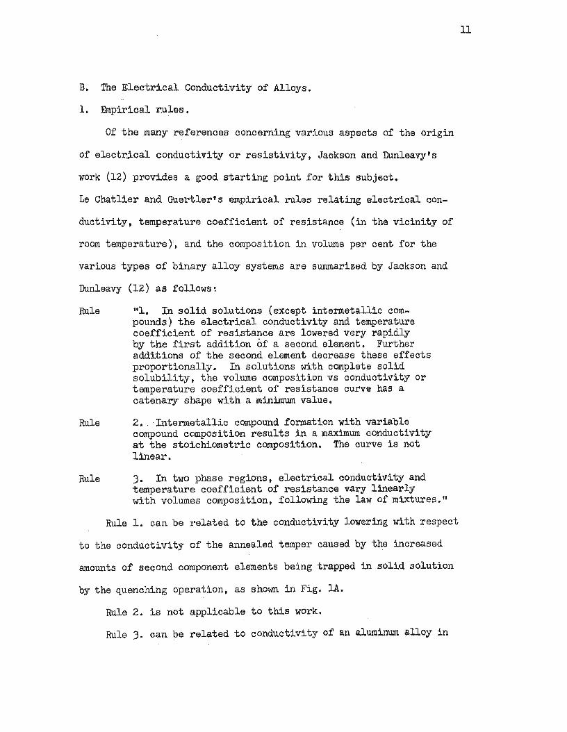
Rule "1. In solid solutions (except intermetallic com­pounds) the elec.trical conductivity and temperature coefficient of resistance are lowered very rapidly by the first addition of a second element. Further additions of the second element decrease these effects proportionally. In solutions with complete solid solubility, the volume composition vs conductivity or temperature coefficient of resistance curve has a catenary shape with a minimum value.

Rule 2. Intermetallic compound formation with variable compound composition results in a maximum conductivity at the stoichiometric composition. The curve is not linear.

Rule 3. In two phase regions, electrical conductivity and temperature coefficient of reSistance vary linearly with volumes oomposition, following the law of mixtures."

Rule 1. can be related to the conductivity lowering with respect

to the conductivity of the annealed temper caused by the increased

amounts of second component elements being trapped in solid solution

by the quenching operation, as shown in Fig. lAo

Rule 2. is not applicable to this work.

Rule 3. can be related to conductivity of ~n aluminum alloy in

11

12

the annealed. temper. It essentially states that the total observed

conductivity is the sum of the conductivities of each phase present in

the alloy. The conductivity contribution of eaoh phase to the total

conductivity is directly proportional to the amount of each phase

present.

In commeroial aluminum alloys, the precipitated phases are gener­

ally intermetallic compounds with relatively fixed compositions. In

addition, the conductivities of intermetallic compounds in aluminum

alloys are quite low when oompared with the conductivity of the matrix

solid solution. Also, the amount of the second phases present is

seldom over ten volume per cent so that the second phase contribution

to the observed total conductivity is quite small. Therefore, the

first assumption made is that the observed conductivity of oommercial

aluminum alloys can be attributed to the conductivity of the aluminum

matrix alone.

Another assumption can be made regarding commercial aluminum

alloys. The so called "impurity elements" are held to rather close

limits and are present in essentially small fixed amounts. Generally,

the impurity elements are not very soluble in the aluminum matrix with

Fe being the principal exception. Often they form stable inter­

metallic compounds. Therefore, their conductivity contributions are

either negligible or essentially constant so that their conductivity

contributions to the total conductivity of the alloy will be ignored.

This assumption when coupled with the prior assumption indioates that

only the all~ng elements which exhibit appreciable increasing solid

solubility with increasing temperature produce Significant conduc-

13

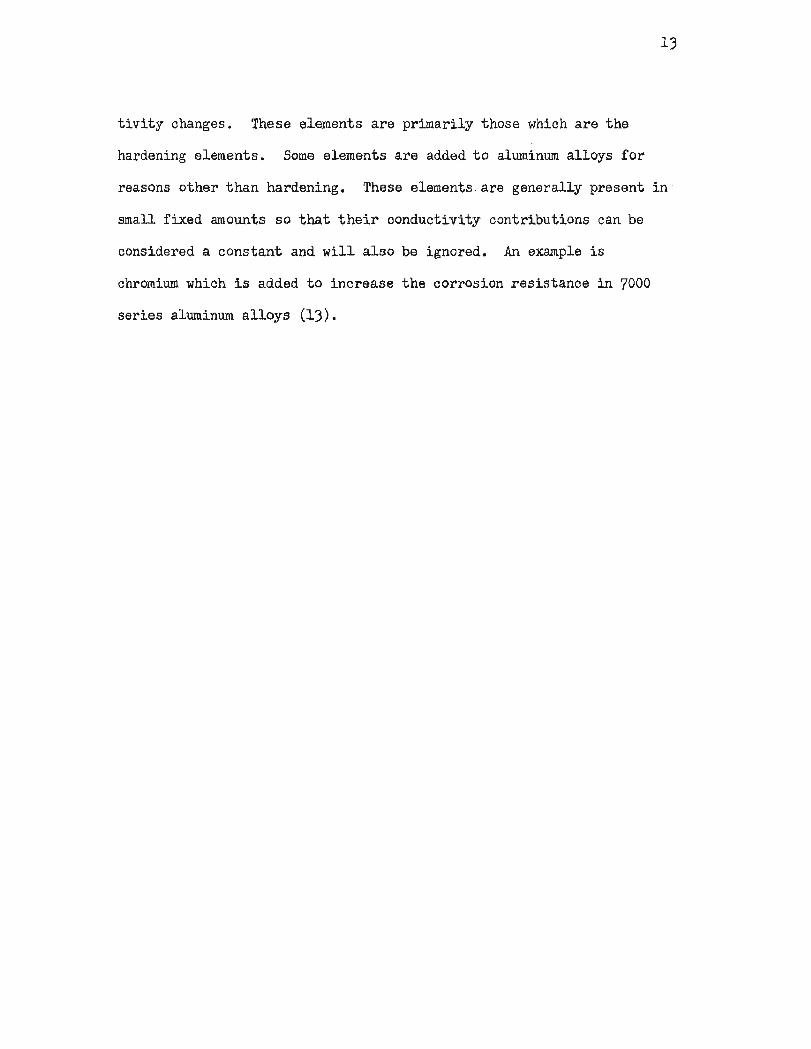
tivity changes. These elements are primarily those which are the

hardening elements. Some elements are added to aluminum alloys for

reasons other than hardening. These elements. are generally present in

small fixed amounts so that their conductivity contributions can be

considered a constant and will also be ignored. An example is

chromium which is added to increase the corrosion resistance in 7000

series aluminum alloys (13).

14

2. Modern theory.

Modern theories of electrical conduction are based upon wave­

mechanics (14, 15). These theories state, in essence, that the elec­

trons move through a metallic crystalline lattice not only as a

particle, but also as electron waves in an electrostatic field. The

electro statio field varies in potential, which can be related to the

periodicity of the lattioe and to the number and type of atoms present

on any given lattice site. A good treatment of the above. the Kronig­

Penney solution for Schrodinger' s wave equation, has been presented by

Azaroff and Brophy (14).

The practical result of the modern theor,y and the first assump­

tion is that the resistivity (or conductivity) of an aluminum alloy

can be related to the periodicity of the aluminum matrix lattice. A

lattice which is perfect~ periodical, such as a pure metal having a

perfect crystal lattice at absolute zero, will allow the electron wave

to travel through the lattice unimpeded. A perfect lattice, in theory,

would have no resistance. The converse is also important. A pertur­

bation in the lattice, which changes the electrostatic potential, will

cause an increase in resistivity. The magnitude of the increase will

be proportional to the amount and type of irregularities present. The

extra resistivity due to conduction electron wave scattering through

lattice interaction can be described by equations which are analogous

to Bragg type X-ray diffraotion equations.*

* Hereafter, this effect will be referred to as "electron

scattering."

3. Factors affecting the conductivity of an alloy.

a) Alloying or impurity elements.

15

Alloying or impurity elements present in the lattice disturb the

periodicity of the lattice (12). The atoms of the alloying phases

generally have a different atomic radius than the parent atoms; there­

fore, a lattice distortion occurs which gives rise to increased

electron scattering, thus decreasing the conductivity. The other main

factor which decreases the conductivity due to increased electron

scattering is the changed electrostatic field about an alloying atom.

A different valence atom at a lattice site has a different electro­

static potential. which changes the periodicity of the lattice at that

site.

The two effects above adequately explain the observed conduc­

tivity decrease of the 7075 alloy in Fig. lA when proceeding from the

annealed temper "0" to the "as quenched" condition, Le., approxi­

mately 46 %r.A.c.s. to 32 %r.A.C.S. respectively. The effects also

help explain w~ the delay quenched samples B and C have higher con­

duotivities than sample A as shown in Fig. 2. The slower cooling

rates trap less alloying elements in supersaturated solid solution,

thus causing less electron soattering. hence higher conductivities.

The effects also indicate that as second phase precipitation occurs

during aging. the conductivity should rise due to the removal of solid

solution atoms from the matrix.

The above effects have been utilized in other ways. e.g., Darn

and Robertson (16) have used the resistivity changes described above

to calculate the valence of aluminum atoms in their lattice and have

arrived at a valence of 2., electrons per metallic bond.

b) Lattice defects.

other factors which will produce electron scattering are lattice

16

defects, i.e., vacancies. interstitial atoms and dislocations. In each

of the three, the lattice period would be altered at the site of their

occurrence. Three references describing lattice defects 'effects upon

the conductivities of alloys are Broom (17), Simmons and Balluffi (18).

and DeSorbo (19). Considering these effects, Jackson and Dunleavy

(12) state:

"The magnitude of these effects is generally small compared with that observed as a result of alloying. The maximum increase in reSistivity produced by extensive hardening of these types is no more than that produced by 0 .l~ of an alloying additive."

Broom (17) found for copper that a change of about 5xl012 dis­

location lines/cm2 corresponds to a change in resistivity equal to

about 0.02 microhm-em. Simmons and Balluffi (18) found the change in

resistivity due to 10-3 vacancies is equal to about 0.01 to 0.001

microhm-em in high purity aluminum. Therefore, the contributions to

an aluminum a1loy's conductivity dUB to these types of lattice defects

are so small that they can be ignored. It is important to note that

these types of lattice defects, per se, are not being ignored. but

only their direct conductivity contributions are being ignored. This

topic is discussed in Section II, C, Special Metallurgical Factors.

c) Ordering.

Other factors affecting the conductivity of alloys are the

effects of long range order and short range order (12). Since long

range order is not involved in this work, attention will be given to

short range order effects. Clustering, a form of short range order,

is closely associated with the early stages of the precipitation

hardening process in aluminum alloys and affects an alloy's

conductivity.

17

Many references covering the formation of Guinier-Preston zones*

and transition precipitates (clustering is closely associated with

the two) during age hardening are available. The morphology and

sequence of occurrence are still somewhat controversial for many

alloys, but several aspects of the above relating to resistivity

changes have been investigated. If a G~P. zone is formed in such a

fashion that it distorts the lattice, then increased amounts of eleo­

tron scattering will occur. That such distortion occurs in a 4~-Al

age hardenable alloy was proven by Nicholson, et aI, through the use

of electron microscopy (20).

Matyas (21) theoretically predicted that the lattice strain and

accompanying valency effect associated with the formation of G.P.

zones and other coherent precipitates would cause a change in

resistivity due to electron scattering. Furthermore, the size and the

number of G.P. zones, and the number, valence and type of atoms in the

G.P. zones all must be considered when predicting the magnitude of the

resistivity changes.

Herman, et aI, (22, 23) and others (24. 25. 26) bear out Matyas'

theory. Asdente (27), however, disagreed. Herman (22) used Matyas'

theory to calculate the critical size of spherical G.P. zones neces­

sary for maximum eleotron scattering for a 5.3 at. %Zn-Al binary alloy.

* Hereafter called "G.P. zones."

18

o Theory predicted a critical size of about 8 A and the size found

o through electron microscopy was 9 A. These sizes are in good agree-

ment and show that clustering increases the resistivity. This is the

cause for the conductivity minimum shown on Fig. lAo Herman, at al,

also states that the critical size is independent of the aging temper­

ature. Therefore, the number of G.P. zones of critical size which are

present at a given aging temperature determines the magnitude of the

conductivity lowering.

Referring again to Fig. lA., it is now possible by analogy to

interpret qualitatively the conductivity minimum occurring in the

earlier stages of aging. Lmnediately after quenching, the conductiv­

ity is lowered to about )2 ~I.A.C.S. due to the change of lattice

period and minor lattice distortion of the now supersaturated solid

solution. As aging begins, clusters form which grow to the critical

size needed for maximum electron scattering. This tends to lower the

conductivity. The matrix is now becoming more periodical due to less

supersaturation, which tends to increase the conductivity~ The

observed conductivity is the integration of these two effects. (See

Herman, Cohen and Fine (22), (page 54). Obviously. since a conduc-

tivity minimum is observed, the clustering-induced conductivity

lowering is the dominant tendency during the earlier stages of aging.

As aging progresses, however, the decreasing supersaturation tendency

becomes dominant. Usually by this time the G.P. zones of critical

size are decreased in number with the remaining G.P. zones either ·

being too large or being transformed into a transition precipitate or .. ,

even into the equilibrium phase, i.e., loss of coherency.

The review of literature and referenoes up to this point provide

adequate practical and theoretical background to interpret or explain

most aspects of conductivity curves of aluminum alloys. When coupled

with the well known trends between hardness changes and precipitation

hardening, conductivity measurements are very useful for quality

control, material processing development, and failure analysis.

Rummel (28) bas summarized these topics for praotical use, but there

are some aspects of conductivity testing whioh are not treated

sufficiently for interpretive consideration. These are retrogression

and lattice imperfection effects upon reaction kinetics and will be

discussed in Section II, C. Special Metallurgical Factors.

d) Temperature effects.

Another factor which will produce conduction electron scattering

is an increase in temperature (12). As the temperature rises the

thermally induced fluctuations of tbe atoms about their lattice

sites ohange the period of the lattice. This results in increased

resistivities. This also changes the temperature coefficient of

resistance, since the entire electrostatic field of the lattice is

changing.

19

Matthiessen's rule states that for dilute solid solutions the

resistivity is campose~ of two portions. One part is due entirely to

thermal effects and the other temperature independent part is attri­

buted to all other effects. The resistivity at absolute zero is

termed the residual resistivity and is considered to be independent of

temperature effects. Precise work and modern theory have shown

Matthiessen's rule to be correct only over small temperature ranges

and then only as a first approximation (29). The temperature coeffi-

cient of resistivity of the residual resistivity does vary with

temperature.

starr has considered portions of the above and found that there

is a definite re~ationship between the conductivity of a solid

solution alloy and its temperature coefficient of resistance as pre-

dieted by Hansen's empirical equation (30). Hansen's equation states

that K = ~ C where K is the conductivity, 0( is the temperature

coefficient of resistance, and Band C are constants.

The physical basis for Hansen's equation is shown below as

derived by starr:

"The resistance of a metal or alloy is defined as: R = p1./A .

where R = resistance in..fl.. (J = resistivity in fA -om. ~ ::z len:gth in em. A = cross sectional area in sq. em.

[Note that his term for resistivity in fA-em is inconsistent.

R should either be in J'.n... or p should be in J'\.-cm.J

Differentiating with respect to temperature and re­arranging terms

(Eq. 4)

(Eq. 6)

whence

dR = d:. = K dP - a RdT dT

Where .~ = temperature coefficient of resistance. K = electrical conductivityljP. a :: linear coefficient of expansion. T = temperature.

'tRewr.::Lting Eq. 2 Hansen's equation as

c( = KC, - C2 Where ~ = 'IB and C2 ~ C/B

20

shows the relationship to Eq. (5) when (dP/dT)= G, and a = G2• That (d~7dT) = C" a constant for a given solute is to be expected for pure metals and dilute solid solutions that obey Matthiessen's rule. Matthiessen's rule states ••• Thus, for anyone alloy· system, dp/ dt is independent of K. and .. can be con­sidered a oonstantfor small changes in solute concentration in dilute solid solution alloys.

The second condition of equality of Eqs. (5) and (6) shows that the constant C2 is simply the linear ooefficient of expansion, Itali • While "a" will vary slightly for different concen~rations of solute in a metal solvent, the change is so small that it can be considered to be a constant and equal to the mean value for all alloys of a series. For an alloy that is heat treatable, the value of Ita" is again essentially in­dependent of the degree of heat treatment and can be considered constant."

starr covers conductivity effects of long range order and short

range order. Fig. 3 is taken from starr's work and in reference to

short range order, starr states:

"In Fig. 2 (jig. 3 in this thesis), where short range ordering or clustering is depicted, the equilib;r:oium. resistance increases with decreaSing temperature. When true equilibrium is attained, the resistance, (and henoe resistivity), change with temperature is negative. Beoause the time to establish equilibrium even in the case of short range ordering or clustering increases exponentially with a decrease in temperature, equilibrium is not established at low temperatures. As a result, experimental curves as shown .in Fig. 2 ~ig. 3) are obtained. That the shape of the ourves of dP/ dT near room temperature is caused by the previous high­temperature heat treatment is readily shown by taking a sample having a negative dP/ dT and heating it to 100°C. and holding it for a prolonged period of time. Since the equilibrium value of resistance in all cases is higher than the experimental values, the resistance should increase during an isothermal test. However. the resistance deoreases continuously during heating to IOOoC. and then remains constant during holding at this low temperature. Thus the change in resistance in this temperature region during the time interval under con­sideration is caused by electron interaction with the lattice and not atom migration ••• "

21

S"hort Range Order

M

R. T • TEMPERATURE FIG. ~. (AFTER STARR)

;: Theoret.i.,oal Curve ---- - Experimental curve

"R.T." - Approximate Room Temperature Position

"M" - Point of Convergence

RESISTANCE VS DEGREE OF SHORT RANGE ORDER

Fig. 3 shows the resistance of the

degree of short range order as a

temperature parameter.

22

starr'S last statement is somewhat confusing. He is alluding

to the conductivity minimum caused by electron scattering of G.P.

zones. Clustering is a diffusion controlled reaction; therefore.

atom migration does occur. The total observed oonductivity is the

integration of the two opposing tendencies as previously stated in

Section II. page 18 of this thesis. However. starr's work is

nevertheless valid.

In reference to Fig 3 and starr's discussion, note that in the

area of room temperature, dP/dT can be both positive and negative

depending upon the prior heat treatment of the sample. Note also·

point 11M" t which represents the small area where the bulk of the

experimental curves merge with the theoretical curve. If point "M"

is in the vicinity of room temperature, then a possibility exists

that samples having equal or nearly equal room temperature conduc­

tivities, but with different prior heat treatments, could be

distinguished from one another by examining their dP/dT curves below

room temperature to see if they diverge.

If point "M" is appreciably above room temperature, then one.

would expect that the dP/dT curves of the two samples would have very

similar slopes. Therefore. any measurable divergence of the curves

would probably occur. if at all. at very low temperatures. Thus a

separation of the samples would be unlikely • . The above statements

assume that the dP/dT curves are straight lines, i.e •• Matthiessen's

Rule is applicable over the temperature range being considered.

If Matthiessen's rule dOes not apply. thana possible means of

separation exists even if pOint ''M'' is significantly above room.

23

24

temperature. This possibility exists because Matthiessen's rule is

always qualified by limiting its use to dilute solid solutions. Many

of the heat treatments used for hardening aluminum alloys produoe

different degrees of supersaturated solid solutions. Therefore. each

sample's dP/dT ourve might exhibit a different temperature dependence,

thus effecting the samples' separation.

If both of the previous methods for effecting a separation of the

two samples do not work, then one would deduce . that point "M" is

appreciably above room temperature and that Matthiessen's rule is

applicable. If Hansen's equation adequately describes the behavior of ·

the aluminum samples, then it becomes possible to measure the conduc­

tivity of a 7178 sample at some known temperature T where T is other

than room temperature. Then by back-calculating using Hansen's or

starr's equation, one can deduce the temperature coefficient of resist­

ance for the sample. This assumes, of course, that Hansen's constants,

Band C, for the 7178 alloy system have been previously determined.

The conductivity of the unknown sample could then be corrected to its

room temperature value for determination of the sample's metallurgical

condition. The inverse calculation could also be made.

Therefore t a significant portion of this theSis will be devoted

to resolving the following questions:

-Is point M in Fig. 3 near room temper~tura for 7178 aluminum

alloys? And if so, can samples with different prior thermal histories

be separated?

-Do 7178 aluminum alloys follow Matthiassen's rule in all heat

treatment conditions? And, if they don't, can samples with similar ·

room temperature conductivities be separated? And if they do, does

Hansen's equation adequately describe their behavior?

25

26

C. Special Metallurgical Factors.

If the thermal history is unknown. or known but is not related to

a standard temper, then the kinetics of the solid state reactions

occurring during precipitation hardening are very important in relating

conductivity and hardness data to metallurgical changes of state. For

oertain heat treatments, the kinetics can be considered to be constant

parameters and thus ignored. However, one can ignore these effects

only if the alloy and its prior thermal histor,y are known and the

thermal histor,r falls under the classification of a standard heat

treatment or common improper heat treatment. Vacancy effects and

retrogression effects are two factors which affect second phase pre­

cipitation reaction kinetios and are discussed in the following

paragraphs.

1. Vacancy effects.

Herman has studied the kinetics of 5 ~ 3 at~Zn-Al binary alloy

during G.P. zone formatiQn(22). He found that early in the aging

process the kinetics of G.P. zone formation are dominated by the type

and number of vacancies present in the lattice. If the vaoancies aid

diffusion of the Zn atoms, then the increased vacancies present

increase the number of growing G.P. zones of critical size for maximum

conductivity lowering early in the aging process. A higher than normal

solution heat treating temperature creates the added number of vacan­

cies needed. A lower than normal solution heat treating temperature

has the opposite effect. All temperatures are above the solvus, so

the effect was not one of changing supersaturation of the matrix.

Herman also found that a much higher solution heat treat temper-

ature produced a reversal in the number of growing G.P. zones. He

speculated that this was caused by some vacancies going to permanent

sinks, possiply a micro-pore, which effectively reduced the number of

vacancies available for aiding Zn diffusion.

It has been found that 7178 bare aluminum alloys have lower con­

ductivities both in the 7.5°F. four day "W' temper and the T6 temper

sub~equent to solution heat treating at 920oF •• when compared with

7178 samples in the two tempers after solution heat treating at the

normal 870°F. solution heat treat temperature ()1). This is in agree-

ment with Hannan's findings. However. there is the possibility that

the higher temperature for solution heat treatment of the 7178 alloy

merely reflects more matrix supersaturation, since the solvus of the

commercial alloy was not known. However, the "as-quenched" conduc-

tivity of samples heat treated at 920°F. is not lower than the "as­

quenched" conductivity of samples heat treated at 870°F., which seems

to preclude different degrees of supersaturation. This effect should

not be ilnportant late in the aging process, because Hennan found that I

vacancy concentration effects were not ilnportant after over-aging.

Therefore. the solution heat treat temperature is a variable to

consider when interpreting hardness vs conductivity data early in the

aging process .becauseof different reaction kinetics attributable to

different vacancy concentrations in the matrix.

27

2. Retrogression effects.

The topics of coherent nucleation and growth, coarsening and

retrogression of second phase precipitates ina parent single phase

matrix are all interrelated phenomena which are still the subject of

much research. Cottrell (15) covers these topics quite well.

Without getting deeply involved in thermodynamic considerations,

retrogression phenomena can be briefly defined or ~xplained in the

follOwing manner: Consider an alloy which has been solution heat

treated and aged at a given temperature, Tl, for a given length Qf

time. Assume that this heat treat cycle has produced a coherent

28

second phase precipitate with a given mean particle size and given dis­

tribution. If this alloy is then subjected to a higher aging tempera­

ture, T2' one would expect some changes to occur with respect to the

precipitate's size, shape and distribution. Since the original pre­

cipitate is coherent, true equilibrium is not established. The higher

aging temperature would increase diffusion rates so that one would

expect solid solution atoms to diffuse towards the precipitate causing

it to grow, which would lower the free energy of the matrix. lfthia

occurs then the precipitate would undergo coarsening.

However, in many instances the particles do not grow, but dis- .

solve into the matrix. If the alloy is held at T2' the now dissolved

atoms may precipitate as a coherent particle, but with a larger size

and different distribution. The new precipitate may even be the non­

coherent equilibrium phase. If the original precipitate dissolves,

then this phenomenon is known as retrogression, restoration or

reversion.

29

Since some second phase precipitates dissolve and others grow,

i.e., retrogress and coarsen respectively, one must be able to explain

why some grow and others do not. This is best explained through the

concept of a critical particle size which is needed before growth can

occur.

Therefore, consider a small coherent precipitate. This precipi­

tate would have a high surface energy and a high strain energy, but a

low chemical free energy, i.e., a low volume free energy. If a solid

solution atom from the matrix were to attach itself to this particle,

the free energy increase because of the added surface and strain

energy would probably not be offset by an equal or greater free energy

decrease of the matrix; therefore, an increase in the system free

energy would result. Thus, the growth of the particle is not favored

from a thermodynamic standpoint. In fact, thermo~amic considerations

dictate that the particle should dissolve.

If the particle does dissolve, then its atoms would be free to

diffuse to another portion of the alloy where a different precipitated

second phase particle may exist. If this precipitate is a much larger

particle, it would have more volume free energy than surface or strain

energy. Therefore, if a solid solution atom were to attach itself to

this new larger particle, then the volume free energy lowering would

be greater than the surface and strain energy .increases. This would

result in a free energy decrease for the system, thus representing a

thermodynamically favored chain of events.

Thus, if the size of the original precipitate was smaller than

the critical size associated with TZ' then retrogression would occur.

If the opposite were true, then coarsening would occur.

The situation is not as simple as stated since the discussion did

not take into account the shape of the particle nor the quantitative

degree of coherency, nor preferred nucleation sites such as grain

boundaries, and many other important considerations. The net result

is that if retrogression occurs and the alloy is held at T2 so that a

new precipitate is formed which has a larger mean size, and different

distribution, then changes should occur in the alloy's hardness and

conductivity.

For example, a larger sized and less finely distributed precipi­

tate should offer less dislocation impediments, hence a lower hardness.

The larger particle size is probably associated with a less super­

saturated matrix, hence a higher conductivity should be apparent due to

less electron scattering.

If the new precipitate produced higher coherency stresses in the

matrix with respect to the original precipitate, a higher hardness and

a changed conductivity might result. This condition often produces

double or even triple hardness peaks on hardness versus aging time

curves.

If the alloy were held at T2 for the proper length of time needed

for retrogression to occur, but for precipitation not to occur, then

the alloy could revert back to a partial solution annealed temper.

This section's topics, if treated fully, could very well become a

major subject of investigation in itself. Furthermore, any experiments

in this area would require experimental techniques to separate the

various conductivity contributions to the total conductivity and also

necessitate a knowledge of particle sizes, shapes and distributions.

Therefore, one must recognize that retrogression effects are to be

expected and should be considered when interpreting hardness vs con­

ductivity data.

III. DISCUSSION

A. General Aspects.

It was decided to work with two alloys. 7178 aluminum alloy was

chosen because it represents a commercial alloy in extensive use

throughout the aerospace industr,y. Also, it is typical of the 7000

series allays. Some limited work was done with a high purity 5% Zn-Al

binary alloy.

The commercial 7178 alloy was obtained in 0.070 inch thick bare

32

sheet stock and sheared into one by two inch samples. All samples were

taken from the same sheet to eliminate, as far as possible, chemical

differences from sample to sample. The binary alloy was contributed as

sheet by the Kaiser Aluminum Corporation and was sheared into similar

sized samples. A spectrochemical check analysis of each alloy is given

below. Kaiser Aluminum Corporation ~alysis for the binary alloy is

also given.

Element

Si Mn CU Mg Zn Cr Fe others AI

Spectrochemistry (~)

7178 Zn-Al Binary

0.12 0.01 Trace N.D.* 1.82 0.04 2.82 No·D. 6 . .5 4.75 0.22 N.D. 0.14 N.D. 0.0.5 N.D. Bal. Bal.

* - Not Determined.

Kaiser Analysis (%)

Zn-Al Binary

0.003 N.D. 0.002

<0.01 4.97 N.D. 0.002

<0.001 Bal.

In order to evaluate the relationships previously discussed, it

was necessar,y to produce several series of samples all with system-

atically varying but known heat treatments. Since quench delays and

common improper heat treatments are relatively straightforward in

interpretation, it was decided to concentrate on different aging

cycles. Samples were heat treated as described in the following

sections.

33

B. Basic Procedures and Equipment.

All solution heat treatments were performed in commercial aluminum

heat treat nitrate salt baths operating to ~ lOaF. of the set tempera­

ture. All quenching was done into cold water with the delay quench

times being about 3 seconds. All aging treatments above room tempera­

ture were performed in a recirculating air furnace with the working

zone at ± 8oF. from the set temperatu~e. All specimens were inserted

into the furnace operating at the set temperature and were air cooled

after aging. A calibrated chromel-a1umel thermocouple with a Rubicon

potentiometer were used to substantiate all aging temperatures. All

room temperature aging was at 75°F. ± 5°F.

All aging times for samples aged above room temperature were

measured from the time they were inserted into the furnace until they

were removed. Aging times for room temperature samples were measured

from the time of quenching until the time that a given measurement was

taken. The precision of aging times was; ± one second for times stated

in seconds; ± five seconds for times stated in minutes up to 60 minutes;

and ± two minutes for all other units of time. One sample which had a

copper-constantan thermocouple imbedded in a hole drilled into the

side of a sample was used to detennine the length of time needed to

achieve a temperature of 250°F. The sample reached 250oF. 210 seconds

after insertion into the furnace •. Therefore, it is estimated that

each sample was at its. aging temperature 255 seconds after insertion

into the furnace, assuming Newton's law of heating applies.

All hardness measurements were the average · of two indentations.

The hardness tests were performed on a calibrated Rockwell Twin Tester.

The conductivity measurements were made using a commercial eddy

current device, called a Conductivity Meter as shown on Illustration

1. It is an Fin-100 meter manufactured by the Magna-Flux Corp. The

principle of operation is as follows: A probe, which is an induction

coil representing one arm of an impedance bridge, is placed on the

material to be measured. Actually t the coil is recessed about .030"

in the probe housing and the housing contacts the material. 'An alter-

nating current in the inductor creates a time varying magnetic field

which induces eddy currents in the material be:lhg tested. " The mutual

inductance between the coil and the samwle estaplishes , a.respense

voltage in ,the coil. This voltage may be reiat'd. to theed~ ~urrents

in the sample material by Lenz law. The net resll1t is that t)!J,e change

of impedance of the test coil and. the response voltage '4.s-pr~~'ortional '. .~ . '.( " , ,.'

to the conductivity of the material. The changed impedance of the

coil upsets the impedance bridge circuit. The bridge is rebalanced

by rotating a variable capacitor.! microammeter is provided as a

null point indicator. ,The variable capacitor is connected to a large

dial which is calibrated directly in ~I.A.C.S. There are. of course,

power supply circuits and other circuits which improve the stability

of the system. The unit is calibrated before each use with known

conductivity standards supplied by the manufacturer.

The precision of the calibration standards are t 3% from N.B.S.

standards. The manufacturer, however, claims that the instrument is

capable of ! It% of the indicated value on the dial; therefore, the

total preciSion of the readings are doubtful on an absolute basis.

However, since the data in this thesis was obtained using one machine

35

ILLUSTRATION 1. - CONDUCTIVITY METERS.

The larger unit shown is the FM-IOO Meter.

The portable unit shown is the FM 120 Meter.

The probes of both units are to the right of

the FM 120 Meter.

36

and one set of calibration standards, relative measurements should be

precise to about It% of the indicated value. A conductivity of 40.0%

will then be 40.0 : 0.6~ I.A.C.S. relative.

37

38

c. 7178 Heat Treatments.

All samples were solution heat treated at 870°F. and water

quenched. Groups of samples were then aged at 75°, 250°, 300°, 350°,

400°, and 450°F. The hardness and conductivity of each sample were

obtained. The results are shown in Tables I and II. The two tables

also show the length of time each sample was aged. The samples aged

at elevated temperatures were permitted to age at room temperature for

at least one week before artificial aging commenced. The one week of

natural aging produced a common starting point condition whioh is

essential~ reproducible for all samples subsequently artificially

aged. This common starting condition is denoted on all hardness vs

conductivity figures as "R.T.". The change of hardness and conduc­

tivity associated with the natural aging at room temperature, 75°F.,

is shown on Fig. 4.

Another group of samples was aged to the T6 temper, (24 hours of

aging at 250°F. after solution heat treating), and then subsequently

re-aged at 450°. 400°, and 350°F. These samples have code numbers

prefixed by aTe, TB, and TA, respectively. The hardness and conduc­

tivity of each sample were obtained. The code numbers and results are

shown in Table III. The re-aging times are also given.

The information contained in Tables I through III is best pre­

sented as hardness vs conductivity graphs. as shown in Figs. 5 and 6

and Figs. 9, 10, 11 and 12, with the latter figures appearing in the

appendix. Fig. 5 is a composite of Figs. 4. 6, 9, 10, 11 and 12.

Aging time or re-aging time is not shown on these graphs, but can be

mentally superimposed on the graphs by remembering that samples having

39

86

- R.T.

78

70

62

54

46

38

30

2~~5----~2L7----~2~9----~31------3~3------3L5----~37

CONDUCTIVITY, % I.A.C.S.

FIG. 4 • . HARDNESS VS CONDUCTIVITY FOR 7178 ALLOY ROOM TEMPERATURE AGE (75 0 F.)t R.T. - POSITION OF 7 DAY @ 75 0 Ft -W­TEMPER.

lOOT

92~

. p:\ 84 ll:: .. (/) til ;

6

R.!_ I 1

\ " . I '- ., \ ..........

\ \

\

\ \ \

\

AGE TEMPERATURE 0 lSOOF.

2S00F. -~- 300°F.

, ~.-:;>' ====0

-.- 350°F /

° • cro 400oF. Ar-IO. 4S0 F.

\

I I I , 1 I I J I I

26 28 ",... 32 34 36 38 40 42 44

CONDUCTIVITY, % I.A.C.S.

FIG. 5. HARDNESS VS CONDUCTIVITY FOR 7178 ALLO~. COMPOSITE OF FIGS. 4, 6, 9, 10, 11 AND 12 PLUS ONE SAMPLE AGED AT 150°F.

g

higher conductivities have longer aging times tor any given tempera-

ture. Also for any given conduotivity. samples aged at lower

temperatures have longer aging times.

As the samples age at room temperature, the oonductivity ap-

proaches a minimum value and the hardness increases as clustering.

i.e., second phase precipitation, occurs. The reasons have been

covered in Section II.. . After about four days of rOom temperature

aging, the rate of G.P. zone formation has slowed so that for all

practical purposes it can be considered zero, (See Fig. 4). SUbse­

quent aging then produces the ourves in Figs. 6, 9, la, 11, and 12.

The following list shows the approximate conductivity and hard-

41

ness associated with the hardness peak attained at each aging tampera-

ture after direct aging from the commonR.T. starting condition.

Aging Temperature . of ·

250 300 3~ ~o 450

Conductivity %r.A.C.S.

32.0 33.5 35.0 36.0 35.0

Peak Hardness RB

94 93 90 88 87

The above values are taken from Fig. 5. This figure represents a

family of aging curves. Note that one sample aged at l50oF. is con­

sistent in its position with its imaginary curve of the family of

curves.

Fig. 5 shows the following trends:

As the aging temperature is decreased

_ the maximum hardness obtainable is increased,

_ the time needed to attain the maximum hardness is increased,

_ the hardn~s6 maximum generally occurs at decreased oonduc-

tivities.

As the aging time and temperature increase

- conductivity approaches, as a limit, its value in the

annealed temper. This value is about 46 %r.A.C.S.

42

Note that the 450°F. hardness peak occurs at lower conductivity

values than what is consistent with other temperature hardness peaks.

This is probably due to resolution of the second phase elements in the

aluminum matrix at 450°F. and subsequent entrapment in solid solution

during the air cool to room temperature.

Referring to the curves in Fig. 6 where the samples were aged

directly at 4500 F. from the starting R.T. condition and the other

group of samples was re-aged from the T6 condition at 450°F., several

trends are evident. When the samples are direct aged from the room

temperature starting condition, the samples at first drop slightly in

hardness and gain slightly in conductivity, e.g., RB 80 to RB 74 and

27% to 29 %r.A.C.S. Samples Dll, Dl and D2 produced this effect.

This effect is also evident in Figs. 9, la, 11 and 12.

Again referring to Fig. 6, one can see that the samples aged at

450oF. from the T6 temper undergo a similar small drop in hardness

with a very small change in conductivity from the values of the T6

temper, e. g., RB 92 to RB 90 and 30 • .5% to 32.8% LA.C.S. Samples

TC1, TC2, and Tell produced the hardness decrease. This decrease on

re-aging is also evident in Figs. 9 and 10. However, a slight recovery

of the hardness is shown as aging progresses at the lower aging

temperatures.

This behavior can be attributed to retrogression effects followed

~ .. !1l C/]

~ <I! ::q

94

86

78

70

62

R.T.

\\ " \ "-\ "-\ "-\

\ \

\ \

\ \

T6

~

\ \

54' \ 25 27 29 31 33 35 37 39

CONDUCTIVITY, % I.A.e.s.

FIG. 6. HARDNESS VS CONDUCTIVITY FOR 7178 ALLOY AGED AT 450°.

• DIRECT AGE X RE-AGE FROM

T6 TEMPER

41 43

~ ~

by reprecipitation of phases which are stable at the new aging

temperature as discussed in the Review of Literature. Herman demon­

strates retrogression effeots in his work with a 5~ At. Zn-Al alloy

(22). The net result is that hardness-conductivity data interpretation

is very difficult if retrogression effects occur due to uncommon heat

treatments. The retrogression effects associated with common

improper heat treatments, however, are predictable and the data

rendered interpretable in most cases.

D. dP/dT Studies.

Interpretation of hardness-conductivity data is possible if the

thermal history of the item in question is known. One must always con­

sider the effects of retrogression and varying solution heat treat

temperatures. However, if one does not know the thermal history, then

difficulties of interpretation develop. Notice that in many instances

a given small range of hardness and conductivity could represent a

sample having one of several different thermal histories. Each of the

thermal histories of each sample in the rectangle on Fig. 5, which 1s

1 %r.A.C.S. units wide and 6 RB units tall, could impart to the sample

different mechanical properties, different corrosion resistances. or

some other important engineering property. Also, one could superimpose

the effects of a quench delay schematically shown in Fig. 2 on other

samples to arrive at the indicated range within the rectangle. There­

fore. it would be desirable to find some nondestructive means of

further identifying the prior heat treatment(s).

As discussed in the Review of Literature, a study of d~/dT

relationships may provide a means of separation of the samples des­

cribed above. Even if a separation is not possible. then Hansen's

equation, if applicable. would provide the basis for developing a

technique of conductivity testing at any outdoor temperature instead

of at room temperature as is now required by many specifications,

e.g., (9).

Certain samples representing several different conductivity ranges

were selected for dp/dT studies. Each range of conductivity was com­

prised of about five to eight samples with a total conductivity spread

of about 1 %I.A.C.S. The ranges selected were around 31, 35 and 38

%I.A.C.S. Several other samples with different conductivities were

also evaluated. Conductivity vs temperature data for the samples

tested is listed in Table IV and was obtained in the following manner

using the experimental apparatus shown in Illustration 2.

46

The 1 x 2 inch samples were affixed to a wooden block. A 28 gauge

copper-constantan thermocouple was placed between the sample and the

wooden bloak. The block was then immersed in a dewar containing dry

ice and methyl alcohol until the tempera~ure of the sample was _BOoF.

or below. Approximately five minutes were required to achieve -BOoF.

The block and samples were then removed from the dewar and allowed to

heat to room temperature.

The temperature was monitored by using a Rubicon porta.ble potenti-

ometer. The temperature compensator contained in the potentiometer was

used instead of an ice water bath for the reference junction. It was

previous~ determined t~t the temperature error would be less than

20F. when using the compensator. This was done by comparing the tem-

perature of boiling distilled water using both the temperature compen-

sator and an ice water reference junction. The temperature of the

boiling distilled water was as shown below.

Referenoe Junction

32°F. - ice water

75°F. - Temperature Compensator

Millivolts

4.26

4.30

Indicated Temperature

As the sample warmed, a conductivity rea.ding was taken in 10°F.

increments by simply placing the probe of the conductivity meter onto

the sample. The clamp acted as a heat sink which allowed the sample

Handle -

Clam.p Hole

Sample

Oonductivity Meter ~.u> ~ 00-0

~ 0 1) ==-= ::::.::. -___ --:-= 0.. 0 CI , 0

potenti·~meterl - Probe

I I I I I

Thermocouple I ___________ . __________ .J

ILLUSTRATION 2

dP/dT APPARATUS

Spring _ o lamp

to warm slowly. The meter was balanced and the conductivity was read

directly in ~I.A.C.S.

48

There are important considerations with regard to precision when

using this technique. The meter probe induces eddy currents into the

sample. This, of course, produces resistance heating which changes the

temperature of the sample as the conductivity measurement is taken.

This temperature error amounts to about 50F. for readings taken below

OOF. Readings taken above OOF.were less affected. Since the meter

detects impedance changes of the probe, which are related to the con­

ductivity of the material being tested, another problem arises. If the

probe changes temperature due to its contact with the cold sample, then

its own impedance may change due to the cooling effect. If a thermal

gradient existed in the sample, the actual t~perature and measured

temperature may not agree giving rise to small conductivity errors,

particularly at lower temperatures.

Therefore, to minimize these errors, the following technique was

used. Several samples were tested to obtain a "feel" for the approxi­

mate conductivities which would be encountered at each temperature.

Then during the actual runs, the meter dial was set to the anticipated

conductivity value for each sample at each temperature so that the

length of time needed to balance the bridge was thus held to a minimum,

less than one second, thus reducing the heating effects upon the sample

and the cooling effects upon the probe. Also, the thermocouple was

placed under the area of probe contact to minimize thermal gradient

errors.

It was readily apparent after plotting the dP/dT curves that one

of the above effects did influence the data in most instances, particu­

larly below OOF. The curves show slightly higher conductivities at low

temperatures than what is consistent with data taken at higher tem­

peratures. Some curves do not show these anomalies.

Since the deviations produce higher conductivities. the resistance

heating effect of the induced eddy currents can be discounted as the

cause since this would produce lower conductivity contributions.

Therefore, it was deduced that either the probe cooling effect or

thermal gradients caused the deViations.

In a separate experiment, the meter was standardized on a 61

%I.A.C.S. standard. The probe was cooled by placing it on a chilled

brass block and the conductivity of the 61% standard was remeasured as

60 ~I.A.C.S.; therefore, indicating that the probe cooling effect would

produce a decreased conductivity error. The probe cooling effect was

discounted as the cause for the deviations leaving small thermal

gradients as the suspected cause. This effect was neglible at tempera­

tures above OOF. Therefore, the practical lower temperature limit of

the apparatus appeared to be about OOF.

As the data in Table IV was plotted, it became apparent that the

samples with very similar room temperature conductivities had very

similar dP/dT curves so that no further interpretation, i.e., sepa­

ration of similar samples, could be accomplished. Fig. 7 shows

typical examples of the d pi dT curves.

The linearity of the dfJ/dT curves indicates that over the tempera­

ture range considered, Matthiessen's rule applies. If very precise

instrumentation could be used to effect a sepa.ration of samples having

7.00

~ 0 6.00 1

~ 0 ~ 0 H

5.001 :.;s

.. ~ H > H 8 4.00 tI.l H I ri)

r~

3.00

2.0Q50

Bll

Bl . TC2

~B2&TA5

------- ------------- __ B6

------------- ~ ~D5

~ ~. ___ Ann.

-30 -10

--------

10 30 50

. 0 TEMPERATURE, C •

~5% Zn-Al

70 90 110

FIG. 7. RESISTIVITY VS TEMPERATURE FOR TYPICAL SAMPLES. THE 5~ ZINC-ALUMINUM ALLOY CURVE IS AN AVERAGE CURVE FOR ALL SAMPLES OF THE ALLOY.

130

\n o

51

the same or nearly the same conductivities, the separation most likely

would be based upon deviations from Matthiessen's rule. The residual

resistivity in Matthiessen's rule can be considered to be the sum­

mation of all conditions producing the residual resistivity. The two

major resistivity contributions are those caused by the matrix solid

solution and those caused by the coherency stresses. If they are

designated Xl and Yl for sample land X2 and Y2 for sample 2, with

each having the same total residual resistivity, then

Xl + Yl = X2 + Y2.

This does not mean that Xl = X2 nor that Yl = Y2, but only that

their sums are equal. This could be the reason why two samples with

different heat treatments can develop the same conductivity at a given

temperature. This hypothesis would also explain why samples with

identical conductivities can have different hardnesses and, very

likely, different mechanical properties. Therefore, any separation

based mostly on conductivity measurements would depend upon the

relative temperature dependence of X and Y in· each sample as pre­

ciselymeasured over a larger temperature range.

The df/dT curves indicate that point "Mil in starr t s graph,

(Fig. 3), is well above room temperature. That point "w' is well

above room temperature is better illustrated in Fig. ? which shows the

same typical curves as Figs. 13, 14 and 15. which are contained in the

. appendix. Fig.? shows that the curves have essentially equivalent

slopes and, therefore, would not converge unless extrapolated well

above room temperature.

The data for several typical samples shown in Fig. 7 were

52

analyzed to determine whether Hansen's equation fits the data. Table

V. shows. in tabular form. the necessary calculations as developed by

Starr, to plot Fig. 8. The linear coefficient of expansion was taken

as an average value of 23.4 x 10-6 em/em/oC. It is also assumed that

dP/dT is equivalent toAf /LlT. Fig. 8 shows that the conductivity vs

temperature coefficient of resistance follows Hansen's equation.

The total equation for the 7178 alloy system is shown below:

K=Bo(,+C

K = 0.00621~ + 0.0819

when K is given in reciprocal microhm-em and ~is given

..n./.n../oc. x 104•

For K given in reciprocal . ,.1l.-cm and eX. given in..().. /...a./oC •• then

B = 0.00621 x 1010 and C = 0.0819 x 106 or K == 0.00621 x 1010 0( +

0.0819 x 106•

Using the above equations or Fig. 8. one only has to measure the

conductivity at any known temperature, calculate or find its corres-

ponding 0< t and correct the conduc:tivity to its room temperature value.

The corrected value thus determined can then be used for conductivity-

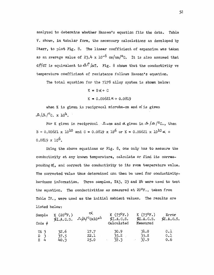
hardness information. Three samples. TA). D3 and E4 were used to test

the equation. The conductivities as measured at 20°F •• taken from

Table IV., were used as the initial ambient values. The results are

listed below:

Sample K (20oF.) eX.. K (7.5°F.) K (75OF.) Error ~I.A.C.S. ~ptj°CxJ..0+4 %r.A. C.S. %I.A. c. S. %I.A. C.S.

Code #: Calculated Measured

TA ) 32.6 17.7 30.9 31.0 0.1 D ) 37.5 22.1 35.2 3.5~2 0.1 E 4 40.3 2.5.0 37.3 37.9 0.6

::s o 0.5 I

&3 o 0:: o H :21 0.4 H < o o ex: Po.. H 0.3 o ~

... l:&:f -.. ~ H > H 8 o

~ o o

0.2

0.1

o

GfL5% Zn-Al

15 17 2l 33 37 4l

TEMPERATURE COEFFICIENT OF RESISTANCE, (eX.), ..n./..n./oCx l04

FIG. 8. CONDUCTIVITY VS TEMPERATURE COEFFICIENT OF RESISTANCE FOR TYPICAL SAMPLES. LINE WAS CONSTRUCTED THROUGH USE OF TEE METHOD OF LEAST SQUARES ANALYSIS.

I..n Iv.)

Note that the errors are 0.1, 0 and 0.6 %r.A.C.S. for samples T3,

D3 and E*. respectively. These errors are within the tolerances of

the conductivity meter itself.

55

E. 5% Zn-Al Heat Treatments.

It was attempted to obtain similar data for the 5% Zn-Al binary

alloy, but unfortunately the alloy was too low in Zn content to achieve

significant hardening, even though the Zn content was approximately the

same per cent by weight as the Zn content of 7075 alloy. The 7000

series alloys, however, contain CU and Mg. These atoms form inter­

metallic compounds such as MgZn2 which can be coherent phases. These

phases evidently are needed to develop the high coherency stresses to

produce the marked change of hardness exhibited in these alloys.

However, df/dT curves were obtained to provide some limited data.

The results of the df/dT tests are shown on Table VI. The procedure

for the conductivity changes with temperature was similar to those used

for the 7178 alloy. The binary alloy samples were annealed for six

hours at 3000 e. and furnace cooled to promote homogeneity in the

samples. The samples were then solution heat treated at 2500 e. for one

hour before water quenching. The solvus for the 5% by weight Zn-Al

binary alloy is approximately 125°C. Herman, Cohen and Fine (22) in

their work with a 5.3 at% Zn-Al binary al10y used solution heat

treating temperatures of both 250°C. and 3000 e. for a length of time

of one hour. After quenching, the samples were affixed to the wooden

block for subsequent dr/dT measurements after aging for the times

indicated in Table VI.

The dP/dT curves for the binary alloy samples formed a band.

Each individual sample's d~/dT curve could not be separated from its

closest neighboring curve; therefore, an average curve is depicted on

Fig. 7 and averaged data is used on Table V to produce the indicated

56

point on Fig. 8. Samples with higher Zn content would have to be used

to develop data similar to that developed for the 7178 alloy samples.

That similar data might be developed is based on the fact that the

de/dT curves are linear over the range tested which indicates that

Matthiessents rule applies; thus, indicating that Hansen's equation

might apply.

57

IV. CONCLUSIONS

The literature survey has shown that modern wave-mechanical

electron conduction theory provides a basis for tbe interpretation of

conductivity changes caused by chemical changes in the composition of

the matrix, which takes place during the heat treatment of aluminum

alloys. Rummel's theory for conductivity-hardness interpretation is

adequate for most practical situations. However, one must consider

the possible occurrence of retrogression effects upon hardness-con­

ductivity relationships and the effects of different solution heat

treating temperatures in conjunction with Rummel's theory for accurate,

logical interpretation of hardness-conductivity data.

The conductivity behavior of the 7178 alloy system can be des­

cribed by Matthiessen's rule and Hansen's empirical equation,

K=BcX+C

A practical result is that the conductivity of any 7178 sample can be

measured at any known temperature and then corrected to its room tem­

perature value for interpretation of the sample's metallurgical con­

dition. The inverse calculation could also be performed. Inverse

calculations could be used to construct a table giving the conduc­

tivity ranges corresponding to tbe standard tempers of the 7178 alloy

at any desired temperature.

POint "M" which is the area of convergence shown on Fig. J seems

to be well above room temperature. This suggests that the resistivity

due to clustering is not close to its theoretical value. However.

this may also mean that the clustering induced resistivity is only a

very small portion of the total observed resistivity. One would have

to be able to separate clustering resistivity effects from the matrix

resistivity effects to truly determine the temperature value of point

"M" with respect to room temperature.

58

No effective separation of samples having similar room tempera­

ture conductivities but different thermal histories could be achieved

through dP/dT studies. Very precise conductivity measurements over a

larger temperature range may produce df/dT curves which show devi­

ations from Matthiessen's rule, thus effecting the samples separation.

The deviations would depend upon the relative temperature dependence

of the two major residual resistivity components, i.e. t the clustering­

induced reSistivity and the matrix resistivity. However, more precise

instrumentation than what was available might also separate samples

having similar room temperature conductivities which appear to be

similar due to the inability of the conductivity meter to distinguish

slight conductivity differences.

It would be interesting if other workers could use the concepts

described in this thesis to evaluate other aluminum alloys, or other

nonaluminum base precipitation hardenable alloys. The concepts of oon­

ductivity testing in general could very well be extended to any

coherent second phase whioh is developed in a parent lattice. Suit­

able allowances would have to be made for the various kinetic effects

of various second phase reactions, e.g., tempering would be a factor

in a transformation hardening alloy system.

Some work has been accomplished in the above area. Conductivity

measurements have been used to follow the omega phase reaction in an

59

8~ Mn-Ti alloy, (32). In this particular application, conductivity

measurements separated samples having too much omega phase from those

with little or none present. The omega phase severely embrittles the

alloy if it is present in quantities above a certain threshold amount.

Other related work, (32), has shown that conductivity testing

concepts, utilizing commercially available eddy current conductivity

meters, did not produce usable results for other titanium alloys.

All of the other titanium. alloys tested had phases which were satu­

rated and/or supersaturated solid solutions at all times. no matter

what the heat treat condition. Therefore, it is speculated that any

resistivity changes caused by the second phase's coherency stresses

are masked by the essentially constant matrix resistivities. No real

effort has been made to date to define the necessary and suffioient

conditions needed for conductivity testing in generalj therefore,

this area would constitute another interesting subject for someone

to explore.

BIBLIOGRAPHY

1. HAGEMAIER, D. (1963) Verification of the -T73 heat treatment of 7075 aluminum alloy by non­destructive methods. Nondestruotive Testing Journal, Sept.-Dot., p. 7-11.

2. HAGEMAIER, D. and KLEINT, R. (1964) Evaluating aluminum alloys by nondestructive tests. Metals Progress, Nov., p. 15-18.

3. VAN DER VELDEN I R. (1965) Determination of aluminum alloy tempers through eleotrical conductivity measurement (.rudy Current) A.erospaoe recom­mended practice. (ARP891), SAE 6-3, Draft 13.

4. COSGROVE, L. (1955) Quality oontrol through nondestructive testing with eddy currents. Nondestruotive Testing, Sept.-Oct.

5. HUNTER, D. and JONES, R. R. and SELTZER, D. D. (1962) Effect of time and temperature exposures on the conductivity and meohanioal properties of 2024-T4 aluminum alloy sheet using eddy current methods. Prooeedings of the Third National Symposium on Nondestructive Testing of Aircraft and Missile Components. Sooiety tor Nondestructive Testing.

6. RUMMEL. W. D. (1966) Characterization and evaluation of 2014 aluminum alloy by eddy current oonduo­tivity teohniques. Materials Evaluation, June. p. 322-326.

7. HAGEMAIER, D. and BASL. G. J. (1967) Evaluation of mechanical properties of 20l4-T6 we1dments by non­destruotive (ed~ currant) methods. Materials Evaluation, Jan •• p. 1-7.

8. HAGl!MAIER t D. (1964) J.ilidy current, hardness t strength relations hips of 2024 aluminum alloy. . Inter­service Data Exchange Program. Report 502.30.l0.00-Gl-Ol, Rocketdyne.

9. Hardness and Conductivity Testing Manual. (Rev. F). McDonnell Co., St. LOOis, Mo.

60

10. MUELLER, R. A. (1965) Conductivity testing of aluminum alloys. McDonnell Co. Process Control Laboratory Report iMAC L 22028.

11. MUELLER, R. A. (1966) 7079 aluminum alloy forging (heat treat inspection). McDonnell Co. Process Control Laboratory Report #MAc L 22308.

12. JACKSON, C. M. and DUNLEAVY, J. G. (1962) The electrical conductivity of metals and alloys. Eleotro­Technology, Science and Engineering Series 41, May, p. 107-114.

13. COOK, M. (1951) Effect of elements in Al-Zn-Mg alloys. J. !nst. of Metals, vol. 79, p. 293.

14. AZAROFF, L. V. and BROPHY, J. J. (1963) Electronic processes in materials. MCGraw-HU1, New York, p. 1-193.

15. COTTRELL, A. H. (1962) Theoretical Structural Metallurgy, 2nd Ed., Edward Arnold, Ltd., London. p. 25-77 and p. 210-221.

16. ROBINSON, A. T. and DORN, J. E. (1951) Trans. Aime, Vol. 191, June, p. 457-460.

17. BROOM, T. (1954) Lattice defects and the electrical resistivity of metals. Advanoes in Physics. vol. 3, p. 26-83.

18. SIMMONS, R. O. and BALLUFFI, R. w. (1960) Measurement of the high-temperature electrical resistance of aluminum: resistivity of lattice vacancies. Physical Review, vol. 117, p. 62-68.

19. DESORBO, W. (1958) Quenched 1m.perfections and the electrical resistivity of aluminum at low temperatures. Physioal Review, vol. 111, Aug., p. 810-812.

20. NICHOLSON, R. B. and NUTTING, J. (1958) Direot observation of the strain field produced by coherent precipitated particles in an age-hardened alloy. Phil. Mag., vol. 3, p. 531-535.

21. MATYAS, Z. (1949) Change of electrical resistance of alloys during aging. Phil. Mag., vol. 40, Mar., p. 324-337.

61

22. HERMAN, H. and COHEN, J. B. and FINE, M. E. (1963) Formation and reversion of Guinier-Preston zones in AI-5.3 at.% Zn. Acta. Met., vol. 11, Jan., p. 43-56.

23. HERMAN, H. (1961) Resistivity changes due to formation of G-P zones. Nature, Vol. 191, p. 63-64.

24. FINE, M. E. (1959) Electrical resistivity change from formation of zones in aluminum alloys. Acta. Met., vol. 7 (3), p. 228-229.

25. HARRISON, W. A. (1960) The effect of solute precipitation on the resistivity of alloys. Acta. Met., vol. 8, No.3, Mar., p. 168-171.

26. MOULD, R. E. andMAPOTHER, D. E. (1961) Effect of precipita­tion hardening on the superconductivity properties of aluminum. Physical Review, vol. 125, Jan., p. 33-43.

27. ASDENTE, M. (1961) Theory of Al-Zn alloy resistivity during pre-precipitation. Acta. Met., vol. 9, June, p. 587-589.

28. RUMMEL, W. D. (1966) Theory of the use of eddy current conductivity devices to monitor alumirnwn alloys. Materials Evaluation, Sept., p • .507-511.

29. ALLEY. P. and SERIN, B. (1959) Deviations from Matthiessen's rule in aluminum, tin, and copper alloys. Physical Review, vol. 116 (2), p. 334-3)8.

30. STARR, C. D. (1963) Correlation of electrical conductivity and resistivity of solid solution alloys with temperature coefficient of resistance. Trans. Aime, Feb., vol. 227, p. 60-64.

31. MUELLER, R. A. (1967) 7000 series aluminum alloys solution heat treated at 920°F. McDonnell Co. Process Control Laboratory Report *MAC 1 22446.

32. MUELLER, R.A. Unpublished work, McDonnel Co., Process Control Laboratory.

62

63

APPENDIX --------

100

92

trl 84 ~ R.T." .. • ~

I

" ~ \ ~ 76 \ ~

~ \ \

6Bl- \

60~

26

"-"-

" _/

\ \

\ \

\ \.

\

T6

'" / /

x

• DIRECT AGE X RE-AGE FROM

T6 TEMPER

28 30 32 34 36 38 40 42

CONDUCTIVITY, ~ I~A.C.S.

FIG. 9. HARDNESS VS CONDUCTIVITY FOR 7178 ALLOY AGED AT 40001'.

0'> +=-

Jl .. til

f2 z

~

96

88

80

72

64

R.T· f I' \ '\. \ "'-\ \ \ \ \ \

\

"

\

"

\ \

T6

~ ~ >f x

)(

x~ •

• DIRECT AGE )( HE-AGE FROM

T6 TEMPER

56' I , ,

26 28 30 32 34 36 38 40

CONDUCTIVITY, % I.A.C.S.

FIG. 10. HARDNESS VS CONDUCTIVITY FOR 7178 ALLOY AGED AT 350oF.

42

0"­\J\

J:Q ~ .. CIl til

~ &:l

~

96

88

80

72

64

T6

FIG. 11.

• DIRECT AGE

• •

CONDUCTIVITY, % I.A.C.B.

HARDNESS VS CONDUCTIVITY FOR 7178 ALLOY AGED AT 3000F.

~ ~

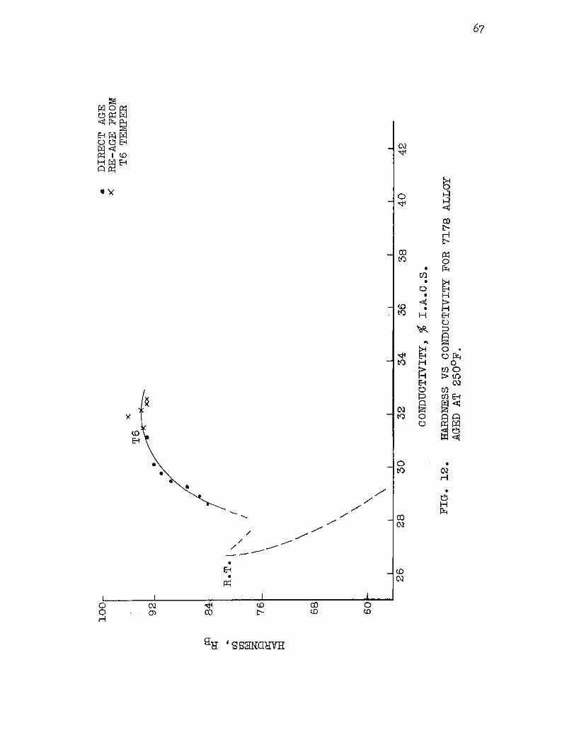
100r • DIRECT AGE >< RE-AGE FROM

x T6 TEMPER T6

92r ~

; rf 84

.. R.T·I" f rf.l rf.l

\ "" / ~ 76 \ ~

~ \ \ \

681- \ \

\ \

60~ \ \

I I 26 28 30 32 34 36 38 40 42

CONDUCTIVITY, % I.A.C.S.

FIG. 12. HARDNESS VS CONDUCTIVITY FOR 7178 ALLOY AGED AT 250°F.

()', ~

36

• O'l 34 •

o •

<4 •

H

~

•

~ 32\ ~ .• ~~ TA5

...:: ~ ~TC2 ~

.. ~ H :::­H 8 o

~ o o

30

28

26

-80 -60 -40 -20

FIG. 13.

o 20 32 40 60

TEMPERATURE, of.

CONDUCTIVITY VB TEMPERATURE FOR SAMPLES INDICATED.

Bl

Bll

80

0'\ co

36

-80 -60 -40 -20

FIG. 14.

2) 32 40 60

TEMPERATURE" of.

CONDUCTIVITY VS TEMPERATURE FOR SAMPLES INDICATED.

100

(j'. '-CJ

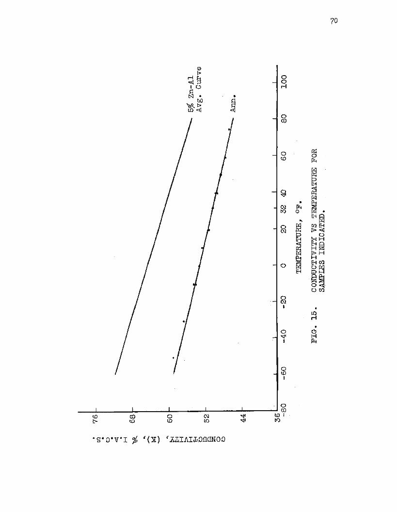
· 76 rIl •

0 •

< • H

~ 68 .. -~ -.. 60 ~ H >

I -H E-t t)

§ 52

0 0

I 44

36' . I .

-80 -60

~ 5% Zn-Al ~ Avg. Curve

------- .

-40 -20

FIG. 15.

o 20 32 .go 60

TEMPERATURE, of.

CONDUCTIVITY VS TEMPERATURE FOR SAMPLES INDICATED.

Ann.

80 100

~ o

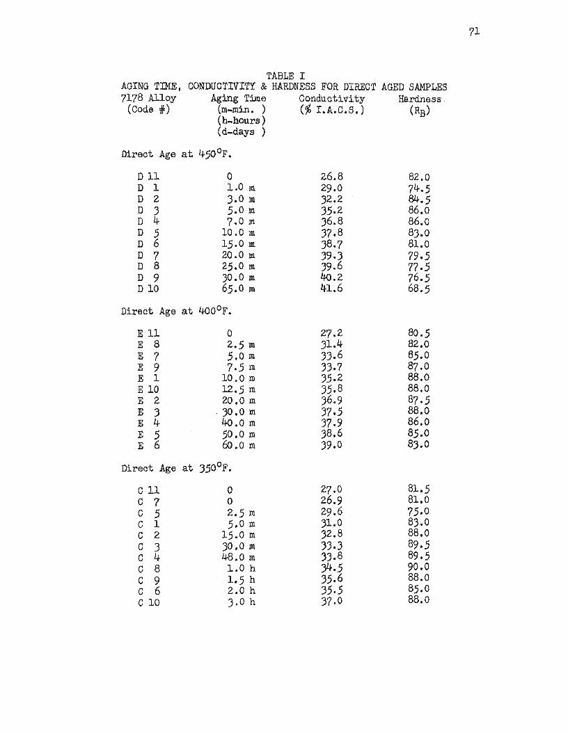
71

TABLE I AGING TDlE. CONDUCTIVITY & HARDNESS FOR DIRECT AGED SAMPLES 7178 Alloy Aging Time Conducti vi ty Hardness .

(Code if) (m-min. ) (% LA.C.S.) (RB) (h-hours) (d-days )

Direct Age at 4,OoF.

D 11 0 26.8 82.0 D 1 l.Om 29.0 74.5 D 2 3.0 In 32.2 84.5 D 3 5.0 m 35.2 86.0 D 4 7.0 In 36.8 86.0 D 5 10.0 In 37.8 83.0 D 6 15.0 m 38.7 81.0 D 7 20.0 m 39.3 79.5 D 8 25.0 m 39.6 77.5 D 9 30.0 m 40.2 76.5 D 10 6,.0 m 41.6 68.5

Direct Age at 400oF.

Ell 0 27.2 80.5 E 8 2.5 m 31.4 82.0 E 7 5.0 In 33.6 85.0 E 9 7.5 m 33.7 87.0 E 1 10.0 m 35·2 88.0 E 10 12.5 m 35.8 88.0 E 2 20.0 m 36.9 87.5 E 3 . )0.0 m 37.5 88.0 E 4 40.0 In 37.9 86.0 E 5 50.0 m 38.6 85.0 E 6 60.0 m 39.0 83.0

Direct Age at 350°F.

C 11 0 27.0 81.5 c 7 0 26.9 81.0 c 5 2.5 In 29.6 75.0 c 1 5.0 m 31.0 83.0 C 2 15.0 In 32.8 88.0 C 3 30.0 In 33.3 89.5 c 4 48.0 m 33. 8 89.5 C 8 l.Oh 34.5 90.0 c 9 1.5 h 35.6 88.0 c 6 2.0 h 35.5 85.0 c 10 3.0 h 37.0 88.0

TABLE I AGING TIME, 7178 Alloy

(Code iF)

CONDUCTIVITY & HARDNESS FOR DIRECT AGED SAMPLES Aging Time Conductivity · Hardness

(m-min. ) (% LA.C.S.) . (Ra) (h-hours) (d-days )

Direct Age at 300°F.

B 11 B 9 B 10 B 1 B 2 B 3 B 4 B 5 B 6 B 7 B 8

o .5.0 m 7.5 m

10.0 In

2.0 h 8.0 h

16.0 h 24.0 h 32.0 h 40.0 h 53. 0 h

26.9 29.7 29.9 29.8 31·5 33.0 33.9 34.8 3.5.2 36.4 37.1

Direct Age at 250oF. (24 Hours Produces T6 Temper)

A 7 A 8 A 9 A 10 A 11 A 12 A 1 A 2 A 3 A 4 A 5 A 6

15. 0 In

30.0 In

60.0 m 2.0 h 3.5 h 5.5 h

24.0 h 2.0 d 3.0 d 4.0 d 5.0 d 6.0 d

Direct Age at 140-16,S°F.

A 11 13.0 d plus l.Oh

28.6 28.9 29.3 29.5 29.8 30.1 31.1 31..5 31.9 32.1 32.4 32.5

29.1

81.0 78.0 77.0 82.5 91.0 93.0 91.5 92.0 90.5 90.5 90.5

84.0 85.0 87.0 89.5 91.0 92.0 93.0 93·5 96.0 94.0 93.0 93·0

93.0

All times in Table I are measured from insertion into the

aging oven. A "0" time indicates at least one week of room

temperature aging at 75°F.

72

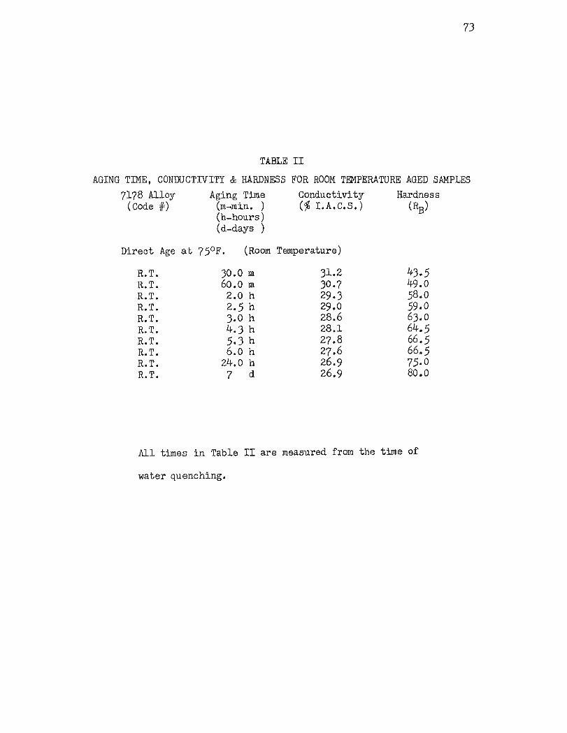
73

TABLE II

AGING TIME, CONDUCTIVITY & HARDNESS FOR ROOM TEMPERATURE AGED SAMPLES

7178 Alloy Aging Time Conductivity Hardness (Code if) (m-min. ) (% 1. A. C. S. ) (Ra)

(h-hours) (d-days )

Direct Age at 750F. (Room Temperature)

R.T. R.T. R.T. R.T. R.T. R.T. R.T. R.T. R.T. R.T.

30.0 m 60.0 m 2.0 h 2.5 h 3.0 h 4.3 h 5.3 h 6.0 h

24.0 h 7 d

31.2 30.7 29.3 29.0 28.6 28.1 27.8 27.6 26.9 26.9

43.5 49.0 58.0 59.0 63.0 64.5 66.5 66.5 75·0 80.0

All times in Table II are measured from the time of

water quenching.

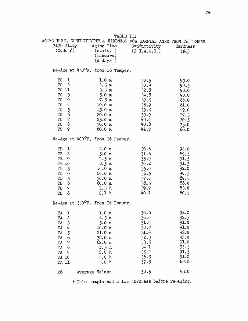
TABLE III AGING TTI1E, CONDUCTIVITY & HARDNESS FOR SAMPLES AGED FROM T6 TEMPER

7178 Alloy Aging Time Conductivity Hardness (Code ~) (m-min. ) (% I.A.C.S.) (RB)

(h-hours) (d-days )

Re-Age at 450°F. from T6 Temper.

TC 1 l.Om 30 • .5 93.0 TC 2 2.5 m 30.9 90.5 TC 11 3.5 m 32.8 90.0 TC 3 5.0 m 34.8 90.0 TC 10 7.5 m 37 • .5 86.0 TC 4 10.0 m 38.9 81.0 TC 5 15.0 m 39.5 79.0 TC 6 20.0 m 39.9 77.5 TC 7 25.0 m 40.4 70.5 TC 8 30.0 m 40.8 73.0 TC 9 60.0 m 41.7 66.0

Re-Age at 400°F. from T6 Temper.

TB 1 2.0 m 30.6 92.0 TB 2 5.0 m 31.6 89.5 TB 9 7.5 m 33·9 91.5 TB 10 8.5 m 34.2 91.5 TB 3 10.0 m 35.0 92.0 TB 4 20.0 m 36.5 90.5 TB 5 30.0 m 37.0 89.5 TB 6 60.0 m 38.5 86.0 TB 7 1.5h 39.7 83.0 TB 8 2.1 h 40.1 80.5

Re-Age at 350°F. from T6 Temper.

TA 1 l.Om 30.6 92.0 TA 2 2.5 m 30.4 92.5 TA :3 5.0 m 31.0 91.0 TA 4 10.0 m 30.9 91.0 TA 5 21.0 m 31.4 92.0 TA 6 38.0 m 32.3 92.0 TA 7 62.0 m 33.5 91.0 TA 8 1.5h 34.1 93.5 TA 9 2.0 h 35.2 91.5 TA 10 3.0 h 36.5 91.0 TA 11 5.0 h 37.5 89.0

T6 Average Values )0·5 93.0

* This sample had a low hardness before re-aging.

TABLE IV

dP/dT DATA FOR 7178 ALLOY SAMPLES

Temperature of.

Code 4F

-60 -50 -40 -30 -20 -10

o 10 20 32 40 50 60 75

-60 -50 -40 -30 -20 -10

o 10 20 32 40 50 60 75

Conductivity (% I. A. C • S • )

Run 1 Run 2

D 3

40.9 4<>.9 40.4 4<>.6 39.9 4<>.1 39.6 39.7 39.3 39.4 38.7 39.0 38.3 38.4 38.0 38.0 37.5 37·5 37.0 :37 .0 36.6 36.6 36.3 36.4 3.5.8 35.8

35.2

E 3

4.5.1 45.0 44.1

43.5 43.1 43.0 42.2 42.4 41.9 41..5 41.4 41.0 41.1 40.6 4<>.5 40.0 39.8 39.4 39.4 39.0 39.0 38 • .5 38.6 38.1 38.1

37.5

Conductivity · (~ LA.C.S.)

Run 1 Run 2

D 5

45.6 45.7 45.1 44.6 44.0 43.0 43.0 42.7 42.7 42.0 42.0 41.5 41.4 41.1 41.0 40.6 40.5 40.0 39.9 39.6 39.5 39.0 38.9 38.6 38.4

37.8

E 4

45.7 46.1 45.0

44.1 44.3 43.4 43.3 42.6 42.6 41.9 42.0 41.5 41.4 41.0 40.8 40.3 40.4 39.8 39.7 39.4 39.4 38.9 38.9 38.4 38.4

37.9

75

Temperature of.

Code #:

~60

-50 -40 -30 -20 -10

o 10 20 32 40 50 60 75

-60 -50 -40 -30 -20 -10

o 10 20 32 .40 50 60 75

76

TABLE IV d(>!dT DATA FOR 7178 ALLOY SAMPLES

Conductivity Conductivity (% LA.C.S.) (% LA.C.S.)

Run 1 Run 2 Run 1 Run 2

E 8 C 1

34.5 34.6 34.7 35.0 34.0 34.2 34.4 34.3 33.6 33.7 34.0 )4.2 33.6 33.6 33.7 33.8 33.2 33.2 33.2 33.0 32.8 32.9 32·9 32 . .5 32.5 32.6 32.7 32·3 32.1 32.3 32.4 31.9 31.8 32.0 32.0 31.6 31.5 31.7 31.8 31.3 31.3 31.4 31.3 31.0 31.0 31.0 31.1 30.7 30.7 30.8 30.7

31.4 31.0

C 10 B 1

43.5 43.7 42.6 42.7 32.8 32.8 42.2 42.2 32.3 32.2 41.8 IH.7 32.0 31.9 41.2 41.0 31.8 31.7 40.5 40.5 31.5 31.4 40.~ 40.1 31.3 31.2 39.7 39.7 30.9 31.0 39.0 39.1 30.6 38.6 38.6 30.2 30.3 38.1 38.3 30.1 30.1 37.8 37.9 29.8 29.9 37.4 37.5 29.5 29 . .5

37.0 · 29.8

77

TABLE IV del dT DATA FOR 7178 ALLOY SAMPLES

Temperature Conductivity Conductivity of. (~ I.A.C.S.) (% I.A.C.S.)

Run 1 Run 2 Run 1 Run 2

Code * B 2 B 5

-60 36.4 )6.3 -50 35.9 35.8 40.0 40.4 -40 35·3 35.3 39.8 39.7 -30 35.0 34.8 39.3 39.1 .. 20 34.6 34.6 38.6 38.7 -10 34.2 34.3 )8.4 38.4

0 33.9 33.8 37.8 37.8 10 33·5 33.5 37.5 37.6 20 33.1 33.1 37.1 37.1 32 )2.8 32.8 36.7 36.5 40 32.5 )2.5 36.4 36.2 50 32.2 32.1 36.0 35.9 60 31.9 31.9 35.4 35.5 75 31.5 34.8

B 6 B 8

... 60 41.5 41.2 44.2 44.1 -50 41.0 41.2 43.2 4}.2 -40 40.5 40.4 42.6 42.7 -30 40.0 42.0 42.0 -20 39.5 39.5 41.6 41.5 -10 39.0 41.1 41.1

0 38.5 38.6 40 • .5 40.6 10 38.0 38.3 40.0 40.0 20 37.6 37.8 39 • .5 39.6 32 37.2 )7.4 39.1 39.1 40 37.0 )7.0 38 • .5 38.6 50 )6.5 )6.5 38.0 38.1 60 36.2 36.2 37.6 37.7 75 3.5.2 37.1

78

TABLE IV de/dT DATA FOR 7178 ALLOY SAMPLES

Temperature Conductivity 'Conductivity of. (% I.A.C.S.) (% I.A.C.S.)

Run 1 Run 2 Run 1 Run 2

Code #: Armealed B 11

-60 -50 59.0 59.0 30.0 30.1 -40 ---- 29.6 29.8 -30 .56.8 56.2 29.6 29 • .5 -20 ---- 29.2 29.2 -10 54 • .5 54.0 28.9 28.9

0 .53 • .5 53.4 28.7 28.6 10 .52.5 52.4 28 • .5 28 • .5 20 .51.0 51.1 28.2 28.2 32 .50.2 49.9 28.0 27.9 40 49.6 49.2 27.7 27.7 50 48 • .5 48 • .5 27.5 27.5 60 47.5 47 • .5 27.3 27.3 75 46.5 26.9

TO 2 A 1

-60 35.0 35·1 35.6 35.5 -50 )4.8 34.7 34.7 35.0 -40 34.1 34 • .5 34.5 34.7 -30 )4.1 34.2 34.3 34.2 -20 34.0 34.0 34.0 -10 33.5 33.5 33.4 33·5

0 33.3 33.1 33.2 33.1 10 33·0 32.9 32.9 32.9 20 32 • .5 32.6 32.6 32 • .5 32 32.3 32.2 32.2 32.2 40 32.0 32.0 32.0 32.0 50 31.7 31 . .5 31.5 31.6 60 31.3 31.3 31.3 31.2 75 30.9 31.1

79

TABLE IV dtJ/dT DATA FOR 7178 ALLOY SAMPLES

Temperature Conductivity Conductivity of. (% I.A.C.S.) (% I.A.C.S.)

Run 1 Run 2 Run 1 Run 2

Code 4F TC 10 TB 2

-60 45.1 45.6 36.4 -50 44.4 4ll-.6 35.6 35.7 -40 43.9 43.5 35.3 35·2 -30 43.2 42.7 35.0 35·0 -20 42.5 42.3 34.6 34.5 -10 41.8 41.9 34.2 34.2

0 41.4 41.5 33.8 33.8 10 40.7 33.5 33 • .5 20 40.1 40.4 33.1 33.2 32 39.7 39.8 32.8 32.7 40 39.3 39.3 32 • .5 32.5 50 38.8 39.0 32.2 32.1 60 38.3 38.5 31.9 32.0 7.5 37.5 31.6

TB .5 TA 3

-60 44.4 44.4 3.5.3 35·7 -50 43.4 43.6 35.0 35.1 -40 43.0 42.6 34.6 34.8 -30 42.2 42.1 34.4- 34.4 -20 41.6 41.5 34.0 -10 41.0 40.9 33.6

0 40.5 40.3 33·3 33.2 10 40.0 40.0 33.0 33·0 20 39.4- 39.5 32.7 32.6 32 39.0 39.1 32.2 32.2 40 38.,5 38.6 31.9 31.9 50 38.0 38.1 31.7 31.7 60 37.6 37.7 31.4 31.3 7.5 37.0 31.0

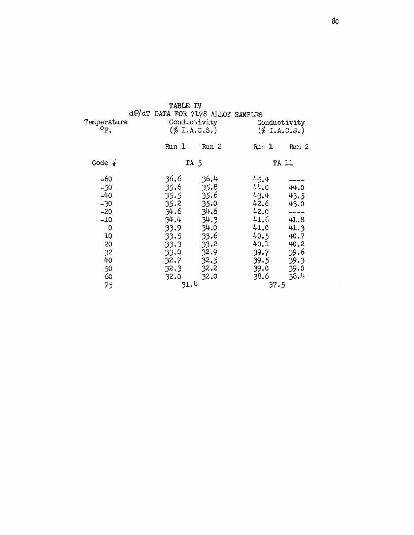
80

TABLE IV dP/dT DATA FOR 7178 ALLOY SAMPLES

Temperature Conductivity Conductivity of. (% I.A.C.S.) (% I.A.C.S.)

Run I Run 2 Run 1 Run 2

Code #= TA 5 TA 11

-60 36.6 36.4 45.4 -50 35.6 35.8 44.0 44.0 -40 35.5 35.6 43.4 43.5 -30 35.2 35.0 42.6 43.0 -20 34.6 )4.6 42.0 -10 34.4 )4.3 41.6 41.8

0 33.9 34.0 41.0 41.3 10 33.5 33.6 40.5 40.7 20 33.3 33.2 40.1 40.2 32 33.0 32.9 39.7 39.6 40 32.7 32.5 39.5 39.3 50 32.3 32 •. 2 39.0 39.0 60 32.0 32.0 38.6 38.4 75 31.4 37.5

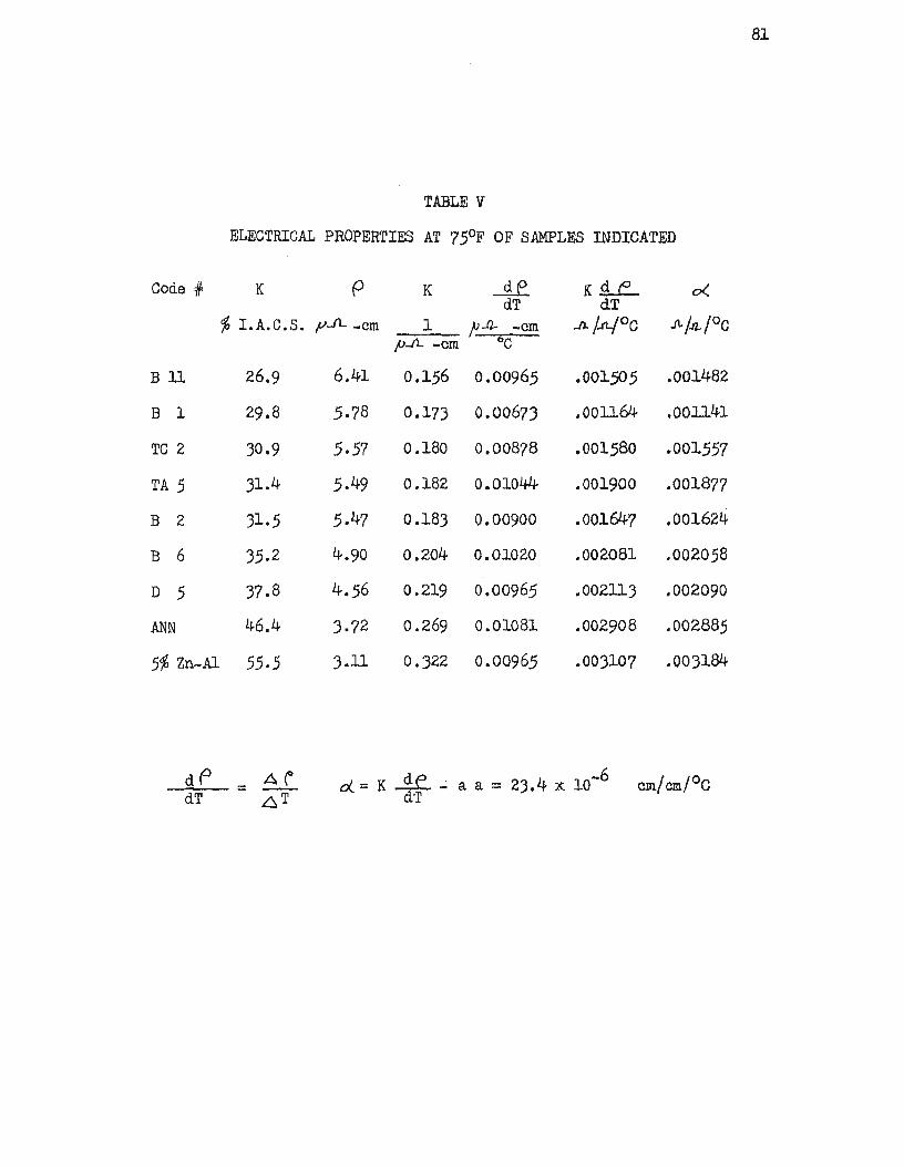
81

TABLE V

ELECTRICAL PROPERTIES AT 75°F OF SAMPLES INDICATED

Code #: K P K ~ K .sLe... 0< dT dT

~ LA.C.S. p.fL -em 1 fJ....Il--CIIl .n. /..tt/°C .fI. /4 /OC p..IL -em 60

B 11 26.9 6.41 0.156 0.00965 .001505 .001482

B 1 29.8 5.78 0.173 0.00673 .OOll64 .001l41

TC 2 30.9 5.57 0.180 0.00878 .001580 .001557

TA 5 31.4 5.49 0.182 0.01044- .001900 .001877

B 2 31.5 5.47 0.183 0.00900 .001647 .001624

B 6 3.5.2 4.90 0.204 0.01020 .002081 .0020.58

D 5 37.8 4 • .56 0.219 0.0096.5 .002113 .002090

ANN 46.4 3.72 0.269 0.01081 .002908 .002885

.5~ Zn-Al 5.5.5 3.ll 0.322 0.00965 .003107 .003184

= A('

~T

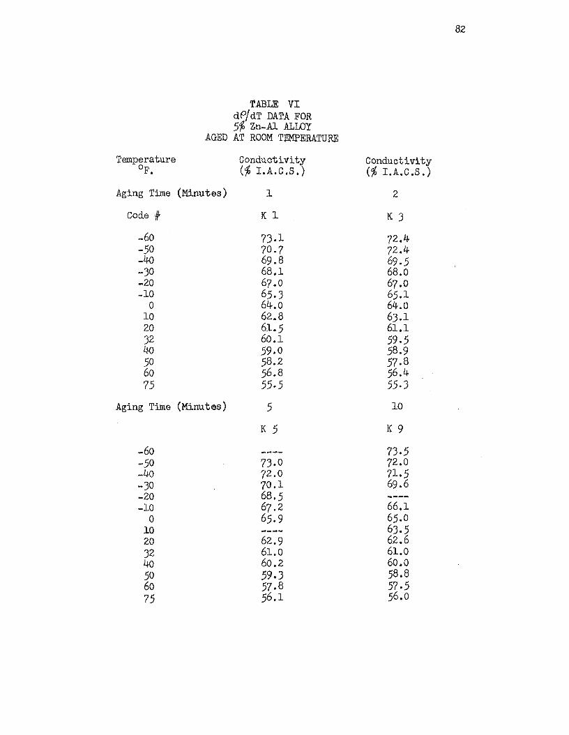
82

TABLE VI dP/dT DATA FOR 5% Zn-Al ALLOY

AGED AT ROOM TEMPERATURE

Temperature Conductivity Conductivity of. (% LA.C ,S.) (% LA.C.S.)

Aging Time (Minutes) 1 2

Code 1F K 1 K 3

-60 73·1 72.4 -50 70.7 72.4 -40 69.8 69.5 -30 68.1 68.0 -20 67.0 67.0 .10 65.3 65.1

0 64.0 64.0 10 62.8 63.1 20 61.5 61.1 32 60.1 59.5 40 59.0 58.9 50 58.2 57.8 60 56.8 .56.4 75 55.5 55.3

Aging Time (Minutes) 5 10

K 5 K 9

-60 73.5 -50 73.0 72.0 -40 72.0 71 • .5 -30 70.1 69.6 -20 68.5 -10 67.2 66.1

0 6.5.9 65.0 10 6) • .5 20 62.9 62.6 32 61.0 61.0 40 60.2 60.0 .50 59.3 58.8 60 .57.8 57 • .5 7.5 .56.1 56.0

83

TABLE VI

df'/dT DATA FOR 5% Zn-Al ALWY

AGED AT ROOM TEMPERATURE

Temperature Conductivity Conductivity Conductivity of. (% LA.C.S.) (% LA.C.S.) (% LA.C.S.)

Aging Time (Minutes) 1.5 2.5 60

Code #= K11 K 7 K 13

-60 74.5 74.3 -50 73.1 71.3 72.0 -40 70.5 70.1 69.6 -30 68.9 68.1 67.4 -20 67.3 68.2 66.5 -10 66.5 65.9 65.2

a 64.9 64.1 63.6 10 63.6 63.0 62 • .5 20 62.6 61.4 61.4 32 60.9 60.1 59.9 40 60.0 .58.8 58.8 50 58.8 57.7 57 • .5 60 .57.6 .56.6 57.0 7.5 56.0 .5.5.4 .55.2

VITA

The author was born on October 9, 1939, in st. Louis, M!ssouri,

where he received his primary and secondary education. He received

a Bachelor of Science Degree in Metallurgical Engineering-Nuclear

Option from the University of Missouri School of Mines and Metal.

lurgy in June, 1962.

He has been enrolled in the part time Graduate School of the

University of Missouri at Rolla - st. Louis Graduate Extension

Center since its inception in September, 1964. He previously was

enrolled in the Graduate School of Washington University, st. Louis,

Missouri.

He is presently employed by the McDonnell Company, st. Louis,

Missouri.

84

12952~