relationships of variables - connected mathematics project

UNIT OVERVIEW

GOALS AND STANDARDS

MATHEMATICS BACKGROUND

UNIT INTRODUCTION

UNIT PROJECT

Mathematics BackgroundRelationships of Variables

One of the central goals of algebra is describing and reasoning about relationships among quantitative variables. That goal has been addressed in many Connected Mathematics Units, as shown in the table below.

Unit Algebra Topic

Gr6 U4 Covering and Surrounding

Gr6 U7 Variables and Patterns

Gr7 U1 Shapes and Designs

Gr7 U5 Moving Straight Ahead,

Gr8 U1 Thinking With MathematicalModels

Gr8 U3 Growing, Growing, Growing

Connections among dimensions,perimeters, areas, and volumesof various figures

General techniques for representing quantitative relationships with words, pictures,tables, graphs, and symbols

Connections among sides andangles in regular polygons

An important family of quantitativerelationships: linear functions thatillustrate constant, additive rates ofchange

Linear patterns of change and howthose patterns contrast with inversepatterns of change

A family of useful nonlinearrelationships: exponential functions, which model exponentialgrowth and exponential decay

This algebra Unit, Growing, Growing, Growing, focuses students’ attention on exponential functions. Studies of biological populations, from bacteria and amoebas to mammals (including humans), often reveal exponential patterns of growth. Such populations may increase over time and at increasing rates of growth. Graphs of the (time, population) data curve upward. This same pattern of growth at increasing rates is seen when money is invested in accounts paying compound interest, or when growth of amoeba is tracked.

continued on next page

15Mathematics Background

CMP14_TG08_U3_UP.indd 15 05/09/13 5:57 PM

Look for these icons that point to enhanced content in Teacher Place

Time

Acc

ou

nt

Val

ue

Time

Pop

ula

tio

n

In a later Unit, Frogs, Fleas, and Painted Cubes, students will study quadratic functions.

The basic goals in Growing, Growing, Growing are for students to learn to recognize situations, data patterns, and graphs that are modeled with exponential functions and to use verbal descriptions, tables, graphs, and equations to answer questions about exponential patterns. This Unit is designed to introduce the topic of exponential functions and to give students a sound, intuitive foundation on which to build later.

Exponential Functions

An exponential pattern of change can often be recognized in a verbal description of a situation or in the pattern of change in a table of (x, y) values.

ApplicationSuppose you offer one of your classes a reward for days on which everyone works diligently for the entire class period. At the start of the year, you put 1 cent in a party fund. You promise that on the first good-work day, you will contribute 2 cents; on the second good-work day, you will contribute 4 cents; and on each succeeding good-work day, you will double the reward of the previous good-work day.

Good-Work Day

0 (start)

1

2

3

4

5

6

7

8

1

2

4

8

16

32

64

128

256

Reward (cents)

Class Party Fund

Growing, Growing, Growing Unit Planning16

Interactive ContentVideo

CMP14_TG08_U3_UP.indd 16 05/09/13 5:57 PM

UNIT OVERVIEW

GOALS AND STANDARDS


UNIT INTRODUCTION

UNIT PROJECT

Growth Factor and Exponential Functions

For each good-work day, the monetary reward doubles. In the table, you multiply the previous reward by 2 to get the new reward. If the x-values increase by 1 unit, this constant factor can also be obtained by dividing each successive y-value by the previous y-value: 21 = 2, 42 = 2, and so on. This ratio is called the growth factor of the pattern. The constant growth factor is the key feature in identifying exponential functions.

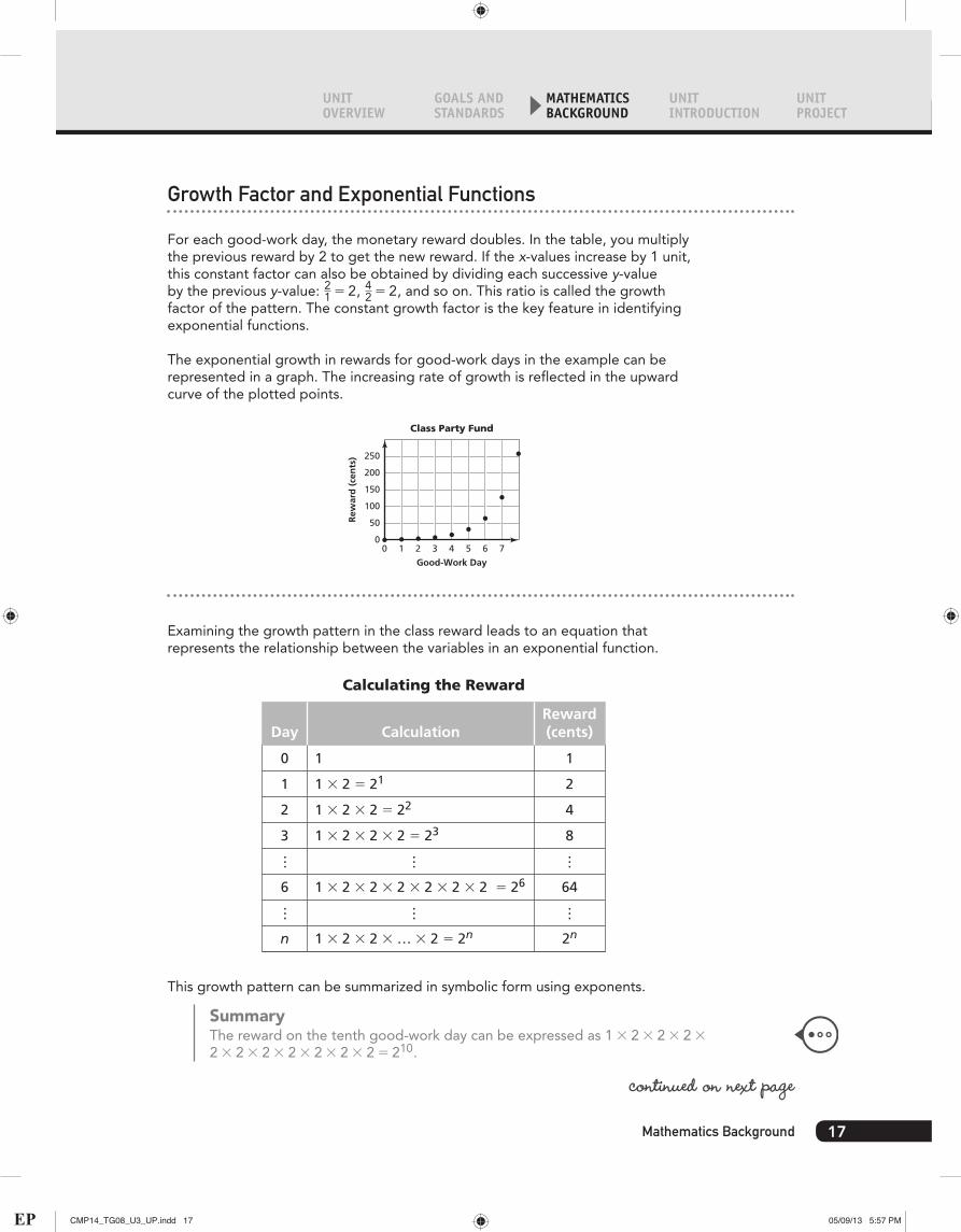
The exponential growth in rewards for good-work days in the example can be represented in a graph. The increasing rate of growth is reflected in the upward curve of the plotted points.

00

50

100

150

200

250

1 3 5 72 4 6

Good-Work Day

Rew

ard

(ce

nts

)

Class Party Fund

Examining the growth pattern in the class reward leads to an equation that represents the relationship between the variables in an exponential function.

Day

0

1

2

3

6

……

……

……

n

CalculationReward(cents)

1

1 × 2 = 21

1 × 2 × 2 = 22

1 × 2 × 2 × 2 = 23

1 × 2 × 2 × 2 × 2 × 2 × 2 = 26

1 × 2 × 2 × … × 2 = 2n

1

2

4

8

64

2n

Calculating the Reward

This growth pattern can be summarized in symbolic form using exponents.

SummaryThe reward on the tenth good-work day can be expressed as 1 * 2 * 2 * 2 * 2 * 2 * 2 * 2 * 2 * 2 * 2 = 210.



CMP14_TG08_U3_UP.indd 17 05/09/13 5:57 PM


On the nth good-work day, the reward r will be r = 2n. Because the independent variable in this pattern appears as an exponent, the growth pattern is called an exponential function, or sometimes just an exponential. The growth factor is the base, 2. The exponent n tells the number of times the 2 is a factor.

y-intercept or Initial Value

The class party fund began with only 1 cent, which means the y-intercept was (0, 1). The following example illustrates a y-intercept that is not equal to 1. Since exponential functions are often used to model situations that involve population growth over time, the y-intercept is also called the initial value.

ApplicationThe class party fund began with only 1 cent. That might strike students as a tiny seed for the fund, so suppose you made a more generous initial offer of 5 cents. The table for this new reward scheme follows; an equation (with the usual variable names, x and y) to represent it is y = 5(2x).

Good-Work Day

0 (start)

1

2

3

4

5

6

5

10

20

40

80

160

320

Reward (cents)

Class Party Fund

Note that the growth factor is still 2. In the table the reward on any given good-work day is twice that of the previous day. The reward is 5 times the reward for the same day in the original scheme, and the new starting amount is reflected in the equation by multiplying the original reward by 5.

The equation for the new plan is y = 5(2x). In the standard form for exponential equations, y = a(bx), a is the y-intercept, and b is the growth factor. Its graph on the next page.



CMP14_TG08_U3_UP.indd 18 05/09/13 5:57 PM

UNIT OVERVIEW

GOALS AND STANDARDS


UNIT INTRODUCTION

UNIT PROJECT

00

50

100

150

200

250

300

1 3 5 72 4 6

Good-Work Day

Rew

ard

(ce

nts

)

Class Party Fund

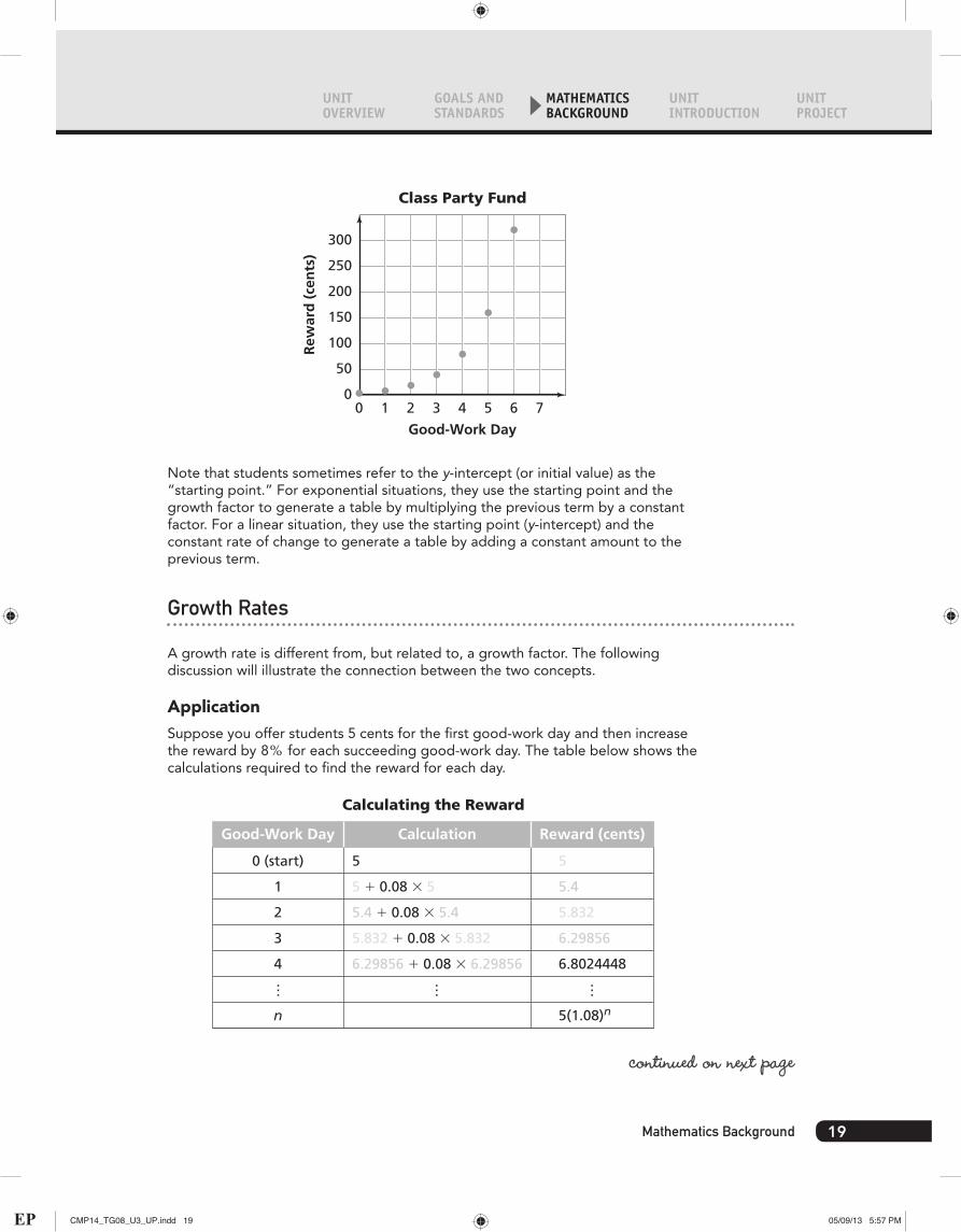
Note that students sometimes refer to the y-intercept (or initial value) as the “starting point.” For exponential situations, they use the starting point and the growth factor to generate a table by multiplying the previous term by a constant factor. For a linear situation, they use the starting point (y-intercept) and the constant rate of change to generate a table by adding a constant amount to the previous term.

Growth Rates

A growth rate is different from, but related to, a growth factor. The following discussion will illustrate the connection between the two concepts.

ApplicationSuppose you offer students 5 cents for the first good-work day and then increase the reward by 8, for each succeeding good-work day. The table below shows the calculations required to find the reward for each day.

Good-Work Day

0 (start)

1

2

3

…

4

n

… …

Calculation Reward (cents)

5

5 + 0.08 × 5

5.4 + 0.08 × 5.4

5.832 + 0.08 × 5.832

6.29856 + 0.08 × 6.29856

5

5.4

5.832

6.29856

6.8024448

5(1.08)n

Calculating the Reward



CMP14_TG08_U3_UP.indd 19 05/09/13 5:57 PM


The 8, increase is the growth rate. By examining the pattern in the reward column, you can see that the growth factor is 1.08. (Divide each reward value by the previous reward value.) The equation for the relationship between the work day n and reward r is r = 5(1.08)n.

Another way to find the growth factor is to apply the Distributive Property at each stage of the calculation, beginning with Day 1 and continuing to Day n.

Day 1: 5 + (0.08 × 5) = 5(1+ 0.08)

= 5 × (1.08)

Day 2: (5 × 1.08) + (0.08 ×(5 × 1.08)) = (5 × 1.08)(1+ 0.08)

= (5 × 1.08)(1.08)

= 5 × (1.08)2

Day n: 5 × (1.08)n

In general, a growth rate of r is associated with a growth factor of (1 + r). Similarly, if the growth factor is f, then the growth rate is (f - 1). Growth rates are often expressed as percents.

Exponential Decay

Exponential Functions also describe patterns in which the value of a dependent variable decreases as time passes. In this case, the constant multiplicative factor is referred to as the decay factor. Decay factors work just like growth factors, only they result in decreasing relationships because they are between 0 and 1.

ApplicationSuppose another teacher offers a different incentive for good-work days. At the start of the school year, the teacher puts +50 in a class party fund. For each day the class does not work diligently, she cuts the party fund in half. As the days pass, the class party fund will decrease in the pattern shown in the following table.



CMP14_TG08_U3_UP.indd 20 05/09/13 5:57 PM

UNIT OVERVIEW

GOALS AND STANDARDS


UNIT INTRODUCTION

UNIT PROJECT

Bad-Work Day

0 (start)

1

2

3

4

5

6

7

8

$50.00

$25.00

$12.50

$6.25

$3.13

$1.56

$0.78

$0.39

$0.20

Reward

Class Party Fund

Notice that, although half the amount is removed at each stage, the amount removed each time decreases.

The exponential decay pattern is also represented in the graph below. The plotted points begin at (0, 50) and drop from left to right.

$5

$10

$15

$20

$25

$30

$35

$40

Class Party Fund

Rew

ard

Bad-Work Day

$45

$50

$00 1 2 3 4 5 6 87

The decay factor for this exponential decay pattern is 12. The amount in the party

fund f after n bad-work days is given by the equation f = 50(12n). This exponential function is similar to that for exponential growth except that the repeating factor, the base, is a positive number less than 1. It is also called an exponential decay function.


CMP14_TG08_U3_UP.indd 21 05/09/13 5:57 PM


Graphs of Exponential Functions

The basic patterns of exponential growth and exponential decay involve change from one point in time to the next by some constant factor.

x

–1 0 1 2 3 4 5

5

10

y

y = 1.5x

x

–1 0 1 2 3 4 5

5

10

y

y = 10(0.7x)

For exponential growth, the change factoris a number greater than 1, and the graphcurves upward from left to right.

For exponential decay, the change factor is between 0 and 1,and the graph curves downward from left to right, approachingthe x-axis but never reaching it.

Exponential relationships can also be defined for negative and noninteger values of the exponent. The related graphs are continuous curves with shapes similar to those shown.

The focus of this Unit is primarily on positive integer exponents, so the graphs will generally be limited to the first quadrant. Rational number exponents are introduced in Investigation 5, but the focus is on the operations with exponents rather than their role in exponential functions. The formal definition of exponential functions for noninteger exponents is delayed until a later course.

Depending on the situation, the graph of an exponential will show discrete points (with or without a curve through the points) or a continuous curve. From Variables and Patterns in grade 6, students will recall the difference between graphs where the dots are connected and those where the dots are not connected. In this Unit, that distinction is not an important one. In fact, it is often useful to connect the dots to highlight a pattern. In such a case, though, it is important to remember that the points corresponding to noninteger values of x may not arise from the data of the problem at hand.



CMP14_TG08_U3_UP.indd 22 05/09/13 5:57 PM

UNIT OVERVIEW

GOALS AND STANDARDS


UNIT INTRODUCTION

UNIT PROJECT

Graph of plotted points Graph of related equation

It is illuminating to occasionally ask students what information the continuous graphs produced by graphing calculators communicate at noninteger points. For example, in many contexts where time is the independent variable, the corresponding y-values have quite natural interpretations.

Equations for Exponential Functions

In general, the equation y = a(bx) represents the relationship in an exponential function; a and b are positive. The y-intercept (or initial value) is a and the growth factor is b. If b is greater than 1, the function is increasing and represents an exponential growth pattern. If b is less than 1, the function is decreasing and represents an exponential decay pattern. If b is equal to 1, then the equation y = a(bx) does not represent an exponential function. It is a linear function with a graph that is a horizontal (slope 0). Visit Teacher Place at Mathdashboard.com/cmp3 to see the image gallery.

2468

1012141618

00 1 2 3 4

y = 2x

y = 1.75x

y = 1.5x

y = 1.25x

x

y

Exponential Growth: 1 6 b



CMP14_TG08_U3_UP.indd 23 05/09/13 5:57 PM


1

2

3

4

00 1 2 3 4

y = 1x

x

y

Constant Function: b = 1

0.10.20.30.40.50.60.70.80.9

00 1 2 3 4

y = 0.75x

y = 0.5xy = 0.25x

x

y

Exponential Decay: 0 6 b 6 1

Students can use tables or graphs to find the value of y if x is known. They can also evaluate the expression y = a(bx). If y is known, then students can use a table or graph to estimate the value of x. In a later course they will develop other methods for finding x, called logarithms. (See the last heading in this section, on logarithms, for more information.)

It is interesting to note that not all problems can be solved by applying standard algorithms. For example, there is no algebraic technique for finding the point of

intersection of an exponential relationship and a linear relationship. y = 12(2x) and

y = 5x + 15. The best we can do is estimate the intersection point of the graphs of the equations. Sophisticated estimation techniques exist, but it is impossible to solve such a problem directly.

Tables for Recursive, or Iterative, Processes

Students usually generate each value in their tables by working with the previous value. Either they add a constant to the previous value (in the case of linear relationships) or they multiply the previous value by a constant (in the case of exponential relationships). This process of generating a value from a previous value is called recursion, or iteration.



CMP14_TG08_U3_UP.indd 24 05/09/13 5:57 PM

UNIT OVERVIEW

GOALS AND STANDARDS


UNIT INTRODUCTION

UNIT PROJECT

Exponential and Linear FunctionsIt is important to distinguish between a constant growth factor (multiplicative), as just illustrated in an exponential function, and the constant additive pattern in linear functions. The animation here illustrates successive iterations for linear and exponential growth. Visit Teacher Place at mathdashboard.com/cmp3 to see the complete animation.

An exponential function represented by the equation y = a(bx) may increase slowly at first but grows at an increasing rate because its growth is multiplicative. The growth factor is b. The y-intercept of the linear function is b and the y-intercept of the exponential functions is a.

Equivalence

In Growing, Growing, Growing, equivalence occurs naturally as students generate two or more symbolic expressions for the dependent variable in an exponential function. Students use patterns from the table, graph, or verbal descriptions to justify the equivalence.

In Investigation 5, after the rules for operation with exponents are developed, students use properties of exponents and operations to demonstrate that two expressions are equivalent.

For example, in the first Investigation of this Unit, students may end up writing two different, but equivalent, exponential equations for this situation.



CMP14_TG08_U3_UP.indd 25 05/09/13 5:57 PM


ApplicationA king places 1 ruba on the first square of a chessboard, 2 rubas on the second square, 4 on the third square, 8 on the fourth square, and so on, until he has covered all 64 squares. Each square has twice as many rubas as the previous square.

By examining the patterns in a table, students write an equation for the number of rubas r on square n.

Square Number

1

2

3

4

5

1

2

4

8

16

Number of Rubas

Rubas on a Chessboard

Some students will note that the number of rubas on a given square n is a product of (n - 1) 2’s and write r = 2n-1.

Other students will reverse the pattern and find the number of rubas on “square 0,” by dividing the number of rubas on square 1 by 2. This gives them the y-intercept, 12. (Square 0 has no meaning in this context, but many students find it useful to use the y-intercept as a starting point when they write an equation.) They then note that the number of rubas on square n is half the product of n 2’s, so they write r = 1

2(2n).

It is important for students to recognize that the two forms, r = 2n-1 and r = 12(2n),

are equivalent. They can verify the equivalence by generating tables or graphs.



CMP14_TG08_U3_UP.indd 26 05/09/13 5:57 PM

UNIT OVERVIEW

GOALS AND STANDARDS


UNIT INTRODUCTION

UNIT PROJECT

Once students have developed the rules for operations with exponents, they can use them to work with exponentials having any value of the growth factor b. (In the chessboard example, b = 2.)

1b

1b

1b

• The equation y = bx–1 is equivalent to y = b x × b–1 .

• Because b –1 = , this is equivalent to y = (bx ) = (bx ).

1b

A general argument why b x–1 is equivalent to (bx ).

Rules of Exponents

Students begin to develop understanding of the rules of exponents by examining patterns in the table of powers for the first 10 whole numbers. Visit Teacher Place at mathdashboard.com/cmp3 to see the complete animation.

The rules for integral exponents are extended to include rational exponents by first noticing that in the graph of y = 4x, the value of y is 2 when x = 1

2. This means

that 14 = 412.

In an interesting optional labsheet, students discover that the ones digits for the powers repeat in cycles of 1, 2, or 4. They apply this observation to predict ones digits of powers and to estimate the value of exponential expressions.


CMP14_TG08_U3_UP.indd 27 03/02/14 7:08 PM


Scientific Notation

Since exponential growth patterns can grow quite fast, students may encounter scientific notation on their calculators. Therefore, scientific notation is introduced in Investigation 1 and then used throughout the Unit. The ACE exercises in every Investigation also continue to reinforce the skills need to work with scientific notation.

ExampleIf you enter (25,000,000,000,000)2, you might get a calculator screen that uses shorthand to indicate the value.

6.25E 26This notation represents 6.25 * 1026.

Sometimes if the numbers are very large or very small, you might get an approximation.

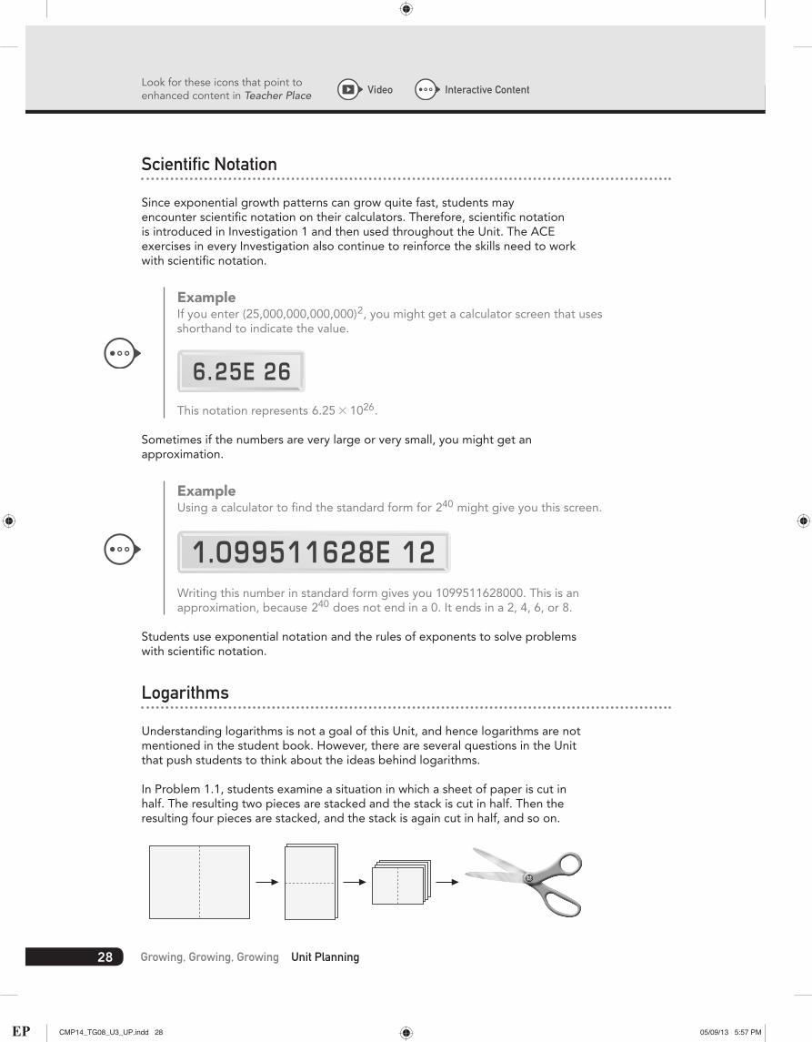
ExampleUsing a calculator to find the standard form for 240 might give you this screen.

1.099511628E 12Writing this number in standard form gives you 1099511628000. This is an approximation, because 240 does not end in a 0. It ends in a 2, 4, 6, or 8.

Students use exponential notation and the rules of exponents to solve problems with scientific notation.

Logarithms

Understanding logarithms is not a goal of this Unit, and hence logarithms are not mentioned in the student book. However, there are several questions in the Unit that push students to think about the ideas behind logarithms.

In Problem 1.1, students examine a situation in which a sheet of paper is cut in half. The resulting two pieces are stacked and the stack is cut in half. Then the resulting four pieces are stacked, and the stack is again cut in half, and so on.



CMP14_TG08_U3_UP.indd 28 05/09/13 5:57 PM

UNIT OVERVIEW

GOALS AND STANDARDS


UNIT INTRODUCTION

UNIT PROJECT

Students write the equation y = 2x to describe the relationship between the number of cuts x and the number of pieces of paper y. In one question, they are asked how many cuts it would take to create at least 500 pieces of paper. The answer is the solution to 500 = 2x.

Students will and should estimate the solution by using a guess-and-check method or by generating a calculator table or graph. In high school, they will learn to use logarithms to solve such an equation exactly.

A logarithmic function is the inverse of an exponential function, just as division is the inverse of multiplication. Taking a base 2 logarithm will undo raising 2 to a power, in the same way that dividing by 2 will undo multiplying by 2. So, taking log2 of both sides of 500 = 2x we get log2500 = x. You can rewrite this equation as x = log2500.

Some calculators can compute logarithms using any base (here the base is 2). Most scientific calculators are limited to the bases 10 and e. In that case, finding a logarithm for base 2 requires several steps.

Example500 = 2x

log10 (500) = log10 (2x)

log10 (500) = xlog10 (2) (by the rules of exponents)

So, .x = log10 500

log10 2

Remember that all of this is far beyond what we ask students to do in this Unit. Logarithms will be addressed in later mathematics courses.

Using Graphing Calculators

Connected Mathematics was developed with the belief that calculators should be available and that students should learn when their use is appropriate. For this reason, we do not designate specific exercises as “calculator exercises.”

Students will need access to graphing calculators for most of their work in this Unit. Ideally, the calculators should be able to display a function table. It is also helpful if you have an overhead display model of the calculator. Extensive exploration of exponential patterns with the assistance of graphing calculators, along with frequent class discussions to share observations and formulate explanations, will add a great deal to the effectiveness of this Unit.



CMP14_TG08_U3_UP.indd 29 05/09/13 5:57 PM


The instructions here are written for the TI-83 graphing calculator. If your students use a different calculator, consult the manual for instruction on these various procedures.

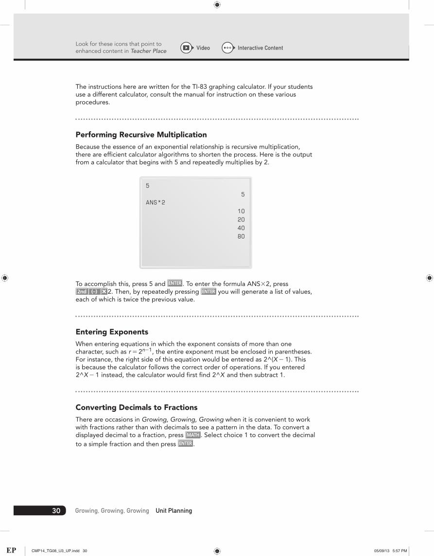
Performing Recursive MultiplicationBecause the essence of an exponential relationship is recursive multiplication, there are efficient calculator algorithms to shorten the process. Here is the output from a calculator that begins with 5 and repeatedly multiplies by 2.

5

ANS*25

10204080

To accomplish this, press 5 and . To enter the formula ANS * 2, press 2. Then, by repeatedly pressing you will generate a list of values,

each of which is twice the previous value.

Entering ExponentsWhen entering equations in which the exponent consists of more than one character, such as r = 2n-1, the entire exponent must be enclosed in parentheses. For instance, the right side of this equation would be entered as 2^(X - 1). This is because the calculator follows the correct order of operations. If you entered 2^X - 1 instead, the calculator would first find 2^X and then subtract 1.

Converting Decimals to FractionsThere are occasions in Growing, Growing, Growing when it is convenient to work with fractions rather than with decimals to see a pattern in the data. To convert a displayed decimal to a fraction, press . Select choice 1 to convert the decimal to a simple fraction and then press .



CMP14_TG08_U3_UP.indd 30 05/09/13 5:57 PM

UNIT OVERVIEW

GOALS AND STANDARDS


UNIT INTRODUCTION

UNIT PROJECT

Displaying a Function TableOnce an equation has been entered, you can display a table of (x, y) pairs that satisfy the equation. The values in the table can be displayed in decimal increments by changing the settings in the TABLE SETUP menu. Press to access the menu and enter a new value for △TBL.

TABLE SETUP TblStart=0 ∆TBL=1Indpnt:Auto AskDepend:Auto Ask

Then press to display the table. Below is a table for the equation y = 1.4x.

X0.1.2.3.4.5.6

Y111.03421.06961.10621.14411.18321.2237

X=0

Entering DataData given as (x, y) pairs can be entered into the calculator and plotted. To enter a list of (x, y) data pairs, press and then press to select the Edit mode. Then enter the pairs into L1 and L2 columns: Enter the first number and press , use the arrow keys to change columns, enter the second number and press , then use the arrow keys to return to the L1 column.

L1

1.099511628E 12

L1 (1)=0

01234

L2 L3 11001803255801050



CMP14_TG08_U3_UP.indd 31 05/09/13 5:57 PM


Plotting the PointsTo plot the data you have entered, use the commands in the STAT PLOT menu. Display the STAT PLOT menu, which looks like the following screen, by pressing .

STAT PLOTS1: Plot1...off L1 L22: Plot2...off L1 L23: Plot3...off L1 L24: PlotsOff

Press to select PLOT1. Use the arrow keys and to move around the screen and highlight the elements shown (ON, icon of discrete points, L1, L2, and open circle for mark).

Plot1 Plot2 Plot3On OffType:

Xllst: L1Yllst: L2Mark: +

Next, press which will display a screen similar to the one below. To accommodate the data you have for input, adjust the window settings by entering values and pressing .

WINDOW Xmin=0 Xmax=5 Xscl=1 Ymin=0 Ymax=1100 Yscl=100 Xres=1



CMP14_TG08_U3_UP.indd 32 05/09/13 5:57 PM

UNIT OVERVIEW

GOALS AND STANDARDS


UNIT INTRODUCTION

UNIT PROJECT

Press .

1.099511628E 12

Exploring Sums of SequencesThe sum of a geometric sequence is a bit beyond what we hope to accomplish in this Unit, but students can use their calculators to derive sums of sequences fairly easily.

The following screen shows how to find the sum of terms in the sequence 2n for n = 0 to n = 10. The calculation involves two operations. The SUM operation gives the sum of all elements in a list. This operation is found in the LIST MATH menu, which is accessed by pressing , selecting MATH, and choosing option 5, sum. (The SEQ operation defines a sequence. This operation is found in the LIST OPS menu. It is accessed by pressing , selecting OPS, and choosing option 5, SEQ.)

sum(seq (2^X, X, 0, 10, 1)) 2047


CMP14_TG08_U3_UP.indd 33 05/09/13 5:57 PM

relationships of variables - connected mathematics project

Documents