relative status indicator development and evolution of a
TRANSCRIPT
RELATIVE STATUS INDICATOR
Development and Evolution of a
Relative Measure of Condition
for Assessing the Status of
Water Quality and Biological Parameters Tracked in the
US/EPA Chesapeake Bay Program Long Term Monitoring
Programs
FINAL REPORT
Prepared by
Marcia Olson
Under contract to
The Interstate Commission for the Potomac River Basin
September 2009

ii
ICPRB Report 09-4
To receive additional copies of this report, please write
Interstate Commission on the Potomac River Basin
51 Monroe St., PE-08
Rockville, MD 20852
or call 301-984-1908.
Disclaimer
The opinions expressed in this report are those of the author and should not be construed
as representing the opinions or policies of the U. S. Government, the U. S. Environmental
Protection Agency, the several states, or the signatories or Commissioners to the
Interstate Commission on the Potomac River Basin.
Acknowledgements
Most of the thinking behind the relative status measure was done by Drs. Alden and
Perry. Dr. Ray Alden left Old Dominion University in 1997. Dr. Elgin Perry continued
to lead the work to its current state in conjunction with other Bay Program partner
analysts. He remains an independent consultant to the Chesapeake Bay Program.
Contact: 2000 Kings Landing Rd, Huntingtown, MD 20639, 410-535-2949,
[email protected]. Thanks also go to Mike Lane at Old Dominion for his interest
in the status method along the way and for taking the time to review and comment on this
document. Funding for this report was provided by the US EPA Chesapeake Bay
Program grant #CB97339103.

1
Introduction
In the Chesapeake Bay region, “Save the Bay” is a bumper-sticker call to action laden
with explicit and implicit meaning. That the Bay needs saving means the Bay is
threatened, it is already changed in some undesirable way or is on the brink of it, and that
the threatened state differs in various respects from our notion of an unthreatened, healthy
Bay. It implies that direct and/or indirect actions undertaken by the sticker-viewing
public can ward off the threat, and the viewer can infer that there are ideas out there about
what those Bay-saving actions are, their beneficial effects, and a vision of what a saved
Chesapeake Bay would look like.
The USEPA Chesapeake Bay Program arose from such a call to action. Under the broad
umbrella of its federal, state and local partnerships, the Bay Program has led efforts to
define quantitatively and qualitatively the conditions implied by the bumper sticker. The
initial work in the late 1970s and early 1980s was to gather available quantitative data
about the Chesapeake Bay environment, to characterize how it was THEN, at some point
in the past, and how it was NOW. The work included hypotheses on the causes of
change and proposals for their reversal. Since then, nutrient and sediment reduction
goals have been set; various restoration goals, habitat requirements and water quality
criteria have been established to define desirable endpoints; and management actions
have been implemented to reduce pollutants, to conserve and protect resources. A long
term monitoring program was established in 1984 to provide ongoing information about
water quality and certain biological groups that are sensitive to water quality changes that
could serve as early indicators of improvement or degradation.
The Chesapeake Bay Program is now 25 years old, and along the way we’ve asked, in
simple bumper-sticker terms: How’s the Bay doing? Are we making progress? The
answer to the deceptively simple questions aren’t simple, and a number of tools have
been developed to grapple with the complexity of the assessments as well as the mixed
results likely to be found in such assessments. Consequently, we have suites of
environmental indicators including, among others, indices of biological integrity, goal
and criteria attainment assessments, trend tests and status measures to help us articulate,
illustrate and contextualize how the Bay and its plant and animal inhabitants are doing--
how they’re coming along.
This paper focuses on the development and application of a relative status measure in the
Chesapeake Bay Program (CBP): the basis of its methodology and lessons learned from
its use in assessing the condition of water quality and biological parameters tracked in the
CBP long term monitoring programs. This status measure has been in use and in the grey
literature of the Bay Program analysts for over a decade, but has not been formally
published previously.

2
Relative versus reference status
The term status in the general sense is the condition of something, its relative position
within a range of conditions. In the context of water quality, for example, status is a
measure of current condition compared to some benchmark or point of reference. If the
reference condition is defined, e.g., if the characteristics of ‘healthy’ water quality were
precisely known, then a status assessment could determine if current water quality
characteristics met, failed or were borderline with respect to those ‘healthy’ reference
characteristics. Regulatory standards, restoration goals and habitat criteria are other
examples of reference points against which reference status assessments can be made.
In fact, in the Chesapeake Bay and its tributaries, precisely defined reference levels are
not available for many water quality and biological parameters, due in large part to the
high temporal and spatial variability inherent in estuaries where land-based fresh water
inputs intersect with salt water from the ocean, the dynamic nature of estuarine biological
processes, and also to the paucity of “pristine”, unaltered habitats in the estuary to serve
as exemplary reference sites. In this circumstance, a measure of relative status can be a
fallback. A relative status assessment determines where a parameter value lies within a
range of observed values. Usually, but not always, one end of the spectrum is believed to
be more desirable than the other and is reflected in the qualitative assessment
terminology. For example, a relative status assessment could determine if current
nutrient concentrations at a site were among the ‘best’ (with lower concentrations) or
‘worst’ (with higher concentrations) of all assessed locations or somewhere in between.
Here, ‘best’ may or may not be equivalent to healthy or desirable and ‘worst’ may or may
not be unhealthy or undesirable. We know only where the site condition lies within the
range of observed conditions.
The CBP measure of relative status
Early version
One of the charges of the group overseeing the CBP Water Quality and Biological
Monitoring Program--then called the CBP Monitoring Subcommittee--was to
communicate to management and the public the state of the Bay and tributaries and
progress toward their restoration. In the mid 1990s, failing reference points for many of
the monitored parameters, the Subcommittee’s Data Analysis Work group (DAWG)
found that it needed a measure of relative status in its assessment toolbox. Two work
group members, Dr. Ray Alden, a statistician at Old Dominion University, and
independent consultant statistician Dr. Elgin Perry proposed such a measure in their
white paper “Presenting Measurements of Status” (1997, Appendix 1). As the title
implies, the proposal includes both a detailed statistical assessment methodology and a
protocol for presenting results that would be easily understood, applicable across
different monitored groups, and would convey comparable qualitative interpretation of
the results across groups. The assessment methodology would be structured so that
positive results represent improvements and negative results represent degradation.

3
Other objectives and desirable characteristics of the status measure are also offered in the
paper.
The authors modified the first draft of the methodology and presentation protocol in
response to input from other work group members and issued a revised version in time
for the method to be exercised in status assessment analyses supporting the 1997 State of
the Bay and Re-Evaluation reports.
In brief, this assessment methodology
• defined a ‘current’ assessment period: the most recent 3-years for which there are
data;
• defined a benchmark or reference period: 1985 through 1996;
• defined ‘habitats’ within which comparisons are made based on salinity and depth
and which are applicable basin-wide;
• defined the most appropriate statistic to be analyzed for status: i.e., the median
value for physical and chemical parameters and the geometric mean value for
biological parameters. These values are computed for each station or segment
within month over the assessment and benchmark periods in order to balance
unequal sampling effort at different times of year. The monthly values are then
assembled to form the assessment and benchmark datasets;
• defined a linear scoring scale from 0 to 100, with 0 representing extreme,
undesirable values and 100 representing extreme desirable values. The scale
endpoints are the parameter’s 5th and 95
th percentile values in the benchmark
dataset within the salinity and depth category and these are assigned respectively
to the undesirable or desirable ends depending on whether low or high values are
desirable for the parameter. The 5th and 95
th percentiles are used instead of the
minimum and maximum values to lessen distortion from outliers. The median or
geometric mean assessment values are scored by proportionally adjusting the
values for representation on the 0-100 scale: e.g., where low values are
undesirable: score = [(value – pct05)/(pct95–pct05)] * 100; and where high values
are undesirable: score = [(value—pct95)/(pct05-pct95)]*100.
• defined the status indicator value for water quality as the median of the median-
based scaled scores in the 3-year assessment period; and for biological data, as
the arithmetic mean of the geometric mean-based scores in the 3-year assessment
period;
• translated the 0-100 numeric scale to a qualitative status measure by dividing the
scale into thirds such that if the indicator value fell in the upper third, the status
was “good”, “fair” if in the middle third and “poor” if in the lower third.;
4
• included a discussion of the influence on the status results of different censoring
strategies for below-detection level (bdl) values and put forward the protocol that
bdl-values be censored at one-half the laboratory method detection limit (MDL)
in place at the time of sample collection. This is in contrast to censoring at the
‘worst’ MDL in place during the assessment and benchmark periods, as is done
for CBP trend analyses.
Complaints, Experiments, Changes
The methodology was revisited over the next several years in light of the status results for
the 1997 reports. That exercise had revealed a number of unsatisfactory aspects to what
later would become known as the ‘linear scoring’ method:
• The benchmark period, 1985-1996, was essentially the full period of record at that
time and included the 1994-1996 three-year assessment period; that is, the
benchmark dataset included the test dataset. If this practice were to continue, then
if an assessment period were particularly bad, the less favorable score would be
mediated by the fact that the relevant endpoint, pct95 or pct05, would also likely
change in the same direction. The user community for this product also asked
that the benchmark period be made constant so that status could be compared
from year to year.
• The final scoring categories--upper, middle and lower thirds—were labeled as
“good”, “fair” and “poor” in order to help convey the scores’ meaning in terms of
environmental condition or health. However, there was no scientific basis for the
association; the categories were relative to the range of data in the benchmark
dataset, not to an empirically desirable endpoint. That disconnect was sometimes
disquietingly apparent.
• Indeed, it was observed that for many parameters--specifically for parameters
with an asymmetric distribution--the distribution of scores among the “good”,
“fair”, “poor” categories was uneven, tending to have more “fair” scores than
seemed right. The expectation for the relative status measure was that the scores
would be more evenly distributed among the categories.
• The collective results for individual stations compared to results for the segment
sometimes didn’t make sense. This seemed best explained by the fact that for
many parameters the variances of space and time are not equal. That is, stations
have only temporal variance, while segments have both temporal and spatial
variance.
A small “ad hoc” team of DAWG members led by Dr. Perry was formed to resolve the
issues. The group chose the 6-year period 1985-1990 as the new benchmark period
because it was early in the monitoring program, long enough to include a wide range of
climatic conditions (e.g., wet/dry years) and short enough to exclude later years in which

5
improvements, if any, from management actions would begin to be reflected in the data.
The choice was made recognizing that as time between the benchmark and assessment
periods increases, the status measure becomes more like a measure of trend. This
problem would have to be revisited sometime in the future.
To solve the asymmetric distribution problem, some research was done to determine the
best transformation for each parameter that would be symmetric and reasonably
approximate some standard statistical distribution. A log transformation produces
symmetry for most water quality parameters, and both the normal and logistic
distributions approximated the distribution of the transformed data as determined by the
probability plot correlation coefficient. The log-logistic was chosen because it is easier to
compute the cumulative distribution function (CDF) of the logistic distribution than for
the normal.
In the revised method, data in both benchmark and assessment datasets are log
transformed. A logistic CDF based on the mean and variance of the parameter in the
benchmark dataset grouped by depth and salinity category is used to perform a
probability integral transform on all parameter values in the benchmark and 3-year
assessment datasets similarly identified by depth and salinity category. Under the
assumption that the logistic distribution is a reasonable model for the log-transformed
data, the probability integral-transformed data in the interval (0,1) follow a uniform
distribution. The median of this 3-year assessment dataset is the status indicator for the
assessment period. For purposes of the status score, the indicator score is scaled to
between 0-100. The scale is divided into thirds and assigned to good-fair-poor categories
as before. This version would be known as the ‘CDF scoring method’. Dr. Perry likened
the procedure of scoring data using the logistic CDF to the classroom procedure of
“grading on a curve” often prayed for by high school and college students. In this case,
the “curve” is set by the mean and variance of the benchmark dataset whereas in
classroom applications, the “curve” is set by the mean and variance of test scores for the
class.
Trials using this CDF method revealed that the majority of scores still fell in the middle
of the range. Dr. Perry suggested two features of the new method that might be to blame,
both having to do with the way variance is computed for the benchmark dataset. One
feature is that the variance used to define the CDF is the variance of individual
observations in the benchmark data. The status indicator is a median of a 3-year period.
A 3-year median should exhibit less variance than individual observations, thus the 3-
year median should be, on average, closer to the center than the individual observations.
It follows that by being closer to the center, the median would fall in the middle category
more often. The second feature which should inflate the frequency of status indicators
falling in the middle category relates to seasonal variance. The variance computed for
the benchmark data and used in the above equation includes a seasonal component that
will make the CDF broader than one that represents the variation of seasonally adjusted
status indicators and result in over-representation of status scores in the middle category.

6
To adjust for seasonal variance, one could compute the variance for the benchmark
dataset with the seasonal trend removed using Analysis of Variance with a seasonal term.
The mean squared error from this ANOVA will estimate variance in the benchmark data
with season removed. This adjustment was ultimately not implemented. Instead, it was
decided to reduce the effects of seasonal variance somewhat by making status
assessments on the seasons most relevant to each parameter (e.g., summer months for
bottom dissolved oxygen, March-October for surface chlorophyll), not necessarily on the
full annual period as had been done previously.
To improve the distribution of the 3-year medians across status categories, i.e., to adjust
for 3-year medians inherently having less variance than the individual observations, an
adjustment factor was applied to the variance of the individual observations. It is known
that if the original data follow a log-logistic distribution, then data transformed as
described above will follow a uniform distribution on the interval (0, 1) (Roussas, 1973).
It is also known that the median of n observations taken from a uniform distribution will
follow a Beta(m,m) distribution where m=(n+1)/2 (Roussas, 1973). Thus, the medians of
the scored data follow a Beta(m,m) distribution. The distribution of 3-year medians from
the benchmark dataset can be partitioned into thirds according to the 66.7 and 33.3
percentiles of this Beta distribution to create the good-fair-poor status categories.
With this modification, the method now produced status assessments spread more evenly
across categories, but with the side-effect of variable cut points for the status categories--
something not easily explained to managers and the public. Using percentiles of the Beta
distribution as the cut points automatically adjusts for differences in sample size (since
m=(n+1)/2). This has the beneficial effect of evening the status results among categories,
but sample size can and does vary systematically and randomly within the Program,
resulting in different cut points, i.e., different definitions of what constitutes good-fair-
poor between assessment groups. It was further found that in most cases serial
dependence of the raw data resulted in the population of 3-year medians having greater
variance than expected if the distribution were Beta(m,m). To adjust for this, the
variance of the Beta density was increased by a function of the ratio of among-station
variance to within-station variance.
This is where the evolution of the CBP’s relative status measure stopped. The CDF
version with these last modifications adjusting for the effect of sample size and serial
correlation were incorporated into the relative status measure computer code (Appendix
2) distributed to Bay Program analysts. While the results became more internally
consistent and comprehensible with these methodological improvements, managers and
communicators remained frustrated by the fact that the relative status endpoints are
obtained from benchmark data and are not grounded in absolute values indicating health
or degradation. As restoration goals and habitat and water quality criteria were
developed within the Program, support for this indicator was discontinued in favor of
those reference-based measures. Relative status assessments may still be part of the suite
of regular reports to management, but they no longer play a major role in communicating
with the public. However, it has been and continues to be a useful tool in exploratory

7
analyses where little is known about the endpoints. Some applications are discussed in
the section below.
Abandoning this assessment approach was short-sighted in this author’s opinion. Dr.
Perry states that there is no reason why the mathematical machinery developed for this
method cannot be reframed as a reference status indicator by specifying the desired mean
and variance for a reference population and scoring the recently observed (test) data
against this reference standard rather than against an existing benchmark dataset. The
challenge remains, of course, to determine or formulate the desired mean and variance of
the reference population, but scoring/assessing a habitat relative to optimal distribution
criteria seems philosophically and scientifically superior to scoring on pass/fail or
distance-from single-point criteria, which is the path the Bay Program chose to take.
Applications of the relative status measure
Although other status measures have supplanted “relative status” as the direct measure of
condition, the methodology has been used in conjunction with other information to
explore and develop first-cut discriminatory categories for reference points:
In the late 1990’s, the Data Analysis Workgroup was working on Environmental
Indicators for total nitrogen and total phosphorus, both of which consisted of a plot of
concentration over time with an overlay of the trend line. They wanted to include a
reference line to indicate what a “healthy” or desirable endpoint concentration would be.
It was recognized that no single concentration could serve for all tidal waters of the
Chesapeake basin nor for all times of year, but healthy restoration levels of nitrogen and
phosphorus had not yet been defined for the various salinity zones and seasons. This
author was asked to research recent and historical nutrient data from the Chesapeake to
come up with empirically derived “healthy” concentrations, which then could be used in
conjunction with experimental data in the literature as basis for the reference lines.
The resulting analysis was documented in a report to DAWG (Olson, 2002). The
approach was first to identify instances of best overall water quality in the long term data
record based on relative status scores of a suite of parameters, then characterize the
nutrient concentrations in these best instances and evaluate them as reference
concentrations. The author believed that a single-parameter approach would not
necessarily yield “healthy” concentrations. In the eutrophic Chesapeake environment,
reducing nutrient loading is the general objective, but lowest concentrations are not
necessarily the same as optimum and low concentrations of a nutrient can occur in both
healthy and unhealthy environments for various reasons. Instead, the author chose to use
the CDF-based relative status assessment of multiple parameters to define and identify
instances of healthy water quality and to use these data to derive the reference
concentrations.
Four parameters were used in the analysis: total nitrogen (TN), total phosphorus (TP),
chlorophyll_a (CHLA) and suspended sediments (TSS). The long term data record
(1950-1999) constituted the test data and these were partitioned by parameter, decade,
8
season, salinity zone and depth layer (in the end, the analysis included only surface data).
Individual parameter values within these groups were scored between 0 and 100
according to the relative status method using the 1985-1990 period for the benchmark
dataset. The median scores within group were assessed as “good”, “fair”, or “poor” using
as status category cut points, the 66.7 and 33.3 percentiles of the Beta distribution of the
corresponding group in the benchmark dataset
Each decade/season/salinity zone was then evaluated to determine if it could represent
“healthy” nutrient and sediment levels. The qualifying rules were arbitrary: none of the
four parameters could have a “poor” assessment; only one parameter could have a “fair”
assessment, one or more parameters had to be “good”. If less than the full suite of four
parameters was available, as often occurred in the pre-1984 years, there was no penalty.
Then, to obtain the reference statistics for each individual parameter, the ‘healthy’ data
pool was further restricted by including only the data in which the status of the parameter
of interest was ‘good.’ Finally, from these “best of the best” data, the mean, median, 10th
and 90th percentiles were computed for each group, with the median serving as the default
proposal for the reference concentration.
The resulting reference concentrations were then compared to good-healthy
concentrations proposed by others. When the TN and TP reference concentrations from
the relative status method were compared to levels derived from nutrient limitation
experiments, it appeared that the relative status reference concentrations for all salinity
zones and seasons were, with one exception, near but still lower than the experimentally
derived levels. The relative status reference concentrations for CHLA and TSS were
considerably lower than maximum concentrations established as CBP restoration
requirements for healthy SAV habitats. As of the date of this publication, no further
action was taken by DAWG to formalize these or other proposals for the nutrient
reference levels. Work on chlorophyll and sediment reference levels continued on a
different track as part of the effort to develop biologically based water quality criteria for
Chesapeake Bay, which focused on chlorophyll, dissolved oxygen and water clarity.
A project to characterize phytoplankton reference communities in Chesapeake Bay
(Buchanan et al., 2005) used the relative status method (in conjunction with
Classification and Regression Tree (CART) analysis (Breiman et al., 1984)) to assist in
classifying samples from impaired and unimpaired phytoplankton habitats. Three
parameters were used in the habitat water quality assessments: concentrations of
dissolved inorganic nitrogen (DIN) and orthophosphate (PO4), and Secchi depth, a
measure of water clarity. The assessment classifications were: Worst, Poor, Better and
Best. Separate assessments were made for different season-salinity zone groupings. The
authors used the relative status method to define classification cutoff points, i.e., to
determine the classification criteria for Worst, Poor, Better and Best classes for Secchi
depth and for Worst nutrient classes. The Best, Better/Poor criteria for the nutrient
classes were not based on relative status scores, but on nutrient concentrations shown to
limit phytoplankton growth in bioassay experiments.

9
Based on the Worst-Poor-Better-Best classification results of the three water quality
parameters, six different classifications were ultimately defined that combined the three
status assessments: 1) Worst light--both nutrients in excess; 2) Poor and Worst light--both
nutrients in excess (including class 1); 3) poor light--mixed nutrient levels including
limiting, 4) better light--excess or mixed nutrient levels, 5) better light--limiting nutrient
levels (including class 6) and 6) best light--limiting nutrient levels. Once these
categories were defined, the long term phytoplankton data record was subjected to a
binning process, in which each phytoplankton sample was assigned to one of the 6
categories based on the classifications of the nutrient and water clarity parameters
measured at the time of sample collection. The data were then grouped by category,
season and salinity zone and the phytoplankton community characteristics of each group
analyzed.
The authors determined that the classification and binning processes were successful in
identifying distinct phytoplankton habitat categories in Chesapeake Bay, and that these
habitats yielded phytoplankton communities that were quantitatively and qualitatively
different from one another when multiple parameters are viewed as a whole. The
habitats with deeper light penetration and limiting or mixed nutrient concentrations
yielded phytoplankton communities with more desirable characteristics (such as
consistently low chlorophyll a and pheophytin concentrations, among others), thus the
communities from these habitats were chosen as the desirable or least-impaired
phytoplankton communities; less desirable communities came from habitats with low
light penetration and higher nutrients. Lacouture et al (2006) expanded on this work,
using the reference communities to develop a Phytoplankton Index of Biotic Integrity (P-
IBI) for Chesapeake Bay and its tributaries. The index is a management tool to assess
phytoplankton community status relative to habitat quality. In a validation exercise, the
P-IBI correctly classified 70.0-84.4% of the impaired and least-impaired samples in the
calibration dataset.
The Buchanan et al. (2005) paper includes a discussion of the validity of the light
classification criteria derived using the Relative Status Method. The authors believe
analyses of some of the phytoplankton community parameters support the light
classification criteria. Elsewhere, it has been shown that the range of chlorophyll a
concentrations as well as chlorophyll cell content (CHL:C) values decrease with
increasing Secchi depth to a point, then level off. In the analyses conducted for this
paper, the Secchi depths where these relationships leveled off corresponded
approximately to the Secchi depth classification criteria from the relative status method.
This is a reminder that the Relative Status Methodology can be very useful as a first cut
approach and that subsequent insights along the way can possibly provide feedback
validation or refinement of the initial results or be, in themselves, a better basis for
different reference points. The “relative” approach is at least a good way to get started.
Supplemental information about the relative status measure is available in several
appendices:

10
• Appendix 1 is the initial paper by Ray Alden and Elgin Perry, “Presenting
Measurements of Status”.
• Appendix 2 contains a SAS® computer program that computes relative status
using the Cumulative Distribution Function (CDF) methodology, including the
last improvements.
• Appendix 3 contains an exchange between Dr. Perry and Mike Lane, a statistician
at Old Dominion University and member of DAWG on the subject of the CDF
method. It includes a brief step-by-step description of the method and schematic
of the assessment process.
• Appendix 4 is an excerpt from a DAWG methods document, “Assumptions and
Procedures for Calculating Water Quality Status and Trends in Tidal Waters of
the Chesapeake Bay and its Tributaries – A cumulative history” which describes
data preparation and method implementation for Bay Program partner analysts.
Note: The Monitoring Subcommittee was supplanted by the Monitoring and Analysis
Subcommittee (MASC) in November 2001; the Data Analysis Work Group (DAWG)
was supplanted by the Tidal Monitoring and Analysis Work Group (TMAW).
References
Alden III, Raymond W. and Elgin Perry. 1997. “Presenting Measurements of Status,” a
white paper prepared for the Data Analysis Work group, Monitoring Subcommittee,
USEPA Chesapeake Bay Program.
Breiman, Leo, J. H. Friedman, R. A. Olshen, and C. J. Stone. (1984)
Classification and Regression Trees. Chapman & Hall, New York.
Buchanan, Claire, Richard V. Lacouture, Harold G. Marshall, Marcia Olson and
Jacqueline M. Johnson. 2005. “Phytoplankton Reference Communities for Chesapeake
Bay and its Tidal Tributaries,” Estuaries Vol. 28, No. 1 p 138-159.
Lacouture, Richard V., Jacqueline M. Johnson, Claire Buchanan, and Harold G.
Marshall. 2006. “ Phytoplankton Index of Biotic Integrity for Chesapeake Bay and its
Tidal Tributaries” Estuaries and Coasts Vol. 29, No. 4, p. 598-616.
Olson, Marcia M. (2002, updated and amended 2009) “Benchmarks for Nitrogen,
Phosphorus, Chlorophyll and Suspended Sediments in Chesapeake Bay”, a white paper
prepared for the Data Analysis Work group, Monitoring Subcommittee, USEPA
Chesapeake Bay Program.
Roussas, George G. (1973) A First Courst in Mathematical Statistics. Addison-Wesley,
Reading, Mass.

Appendices
Pg - 1
Appendix 1
Presenting Measurements of Status
Prepared for the
Chesapeake Bay Program Data Analysis Workgroup
by
R. W. Alden III and E. Perry


Appendices
pg 17
Appendix 2
SAS Language Computer Program (STATMAC.SAS)
to Compute Relative Status Indicator

Appendices
pg 18
************************************************************************** statmac(4) .SAS A macro to compute status based on logit centiles of the benchmark data set. programmer: Elgin S. Perry, Ph. D. date: 4/99 Modified by Marcia Olson, 5/99,and again 6/2000 to provide status reports for stations and segments. Note: her modifications are NOT to the fundamental method of determinng Relative Status. address: 2000 Kings Landing Rd. Huntingtown, Md. 20639 voice phone: (410)535-2949 fax/modem: (410)257-2937 (by arrangement on voice line) email: [email protected] ************************************************************************** Documentation -- The user must supply a benchmark data set and a monitoring data set. The macro assumes that both SEGMENT and STATION identifiers are in both data sets, and the user must indicate whether status is to be scored by segment or by station. The user must indicate the period within that monitoring data set for which status is to be evaluated, a variable defining salinity zone, a depth zone variable, which can be any set of categories, a parameter to evaluate (name must be the same in benchmark and monitoring data), "GOOD" or "BAD" depending on whether high values of the parameter are rated as good or bad, a filename for an external results file, and the units of the untransformed parameter. If no external file is to be created a dummy name should be entered. The variable for defining salinity zone can be based on fixed station or segment zones or sample salinity. It must be defined by the user in both the monitoring and the benchmark data before calling this macro, and the variable name for salinity zone must be the same in both data sets. There could be an option for using the salinity zone implied in the segment name if other salinity designation is not available. The macro assumes that benchmark and status data sets are similarly summarized prior to input. As written, the macro assumes that data are summarized by station year month and depth-zone, and median calculations are made with all data pooled by segment or station and depth-zone without further summarization. If individual sample values are included in the data sets, then the additional step to calculate median values by month (to improve the seasonal balance of the data) needs to be added to the code, before the median score is calculated. On completion, the macro can produce several kinds of output: 1) a print file for data checking with the values of intermediate variables, cut points and status, and the distribution within status categories, 2) a formatted formal results table with a limited number of variables and status, and 3) a comma-delimited ascii file of results. The user may select any or all them by adding or removing the asterisk preceding the macro call. STATSTAT - is a final data set that has a record for each station or segment with the variables: SEGMENT, STATION (if selected), &layvar N, MEDVALU CUT1, CUT2, MEDSCORE, STATUS. MEDVALU - is the median value of the original, untransformed parameter

Appendices
pg 19
MEDSCORE - is the median score for the status period CUT1 - is the 1/3 centile=poor-fair cutpoint if a high score for param is good, or fair-good, if a high score is bad. CUT2 - is the 2/3 centile=fair-good cutpoint if a high score for param is good, or poor-fair, if a high score is bad. STATUS - is the status rating Arguments for the macro STATUS (segsta,bmdata,mondata,statper,salvar,layvar,param,gob,filenam). &segsta is either SEGMENT or STATION, Upper Case sensitive &bmdata is the input benchmark data set &mondata is the monitoring data set &statper is a boolean expression that defines the status period eg ('01jan96'd <= date <= '31dec98') &salvar is the variable name for salinity regimes &layvar is the variable name for layers ¶m is the parameter being evaluated &gob is a variable that indicates whether high values of the parameter are Good Or Bad. Enter good or bad. &filenam is the name of an output text file. &unit is the units of measure of the original parameter, for example ug/L for CHLA, mg/L for TN, and m for Secchi depth. Search for "Edit" to find the lines of code which require User input. End of documentation ; */ options CENTER linesize = 78 pagesize = 55 replace ; option symbolgen MPRINT; *Option to Print out raw information for internal use; %MACRO PRNTRAW (data); PROC SORT DATA=&data OUT=PRNT; BY descending &layvar; PROC FREQ DATA=PRNT; by descending &layvar; TITLE "Distribution of categories for ¶m by &bycat and layer"; TITLE2 "Assessment period &statper, Season = &seas"; TABLES STATUS; RUN; * PROC PRINT DATA=&data; * TITLE "Statistics for ¶m by &bycat" ; * VAR SEGMENT &bycat &layvar N B AN F MEDSCORE CUT1 CUT2 STATUS; %MEND; %MACRO STAT; ** A submacro of the macro STEP1; * find median score by segment or station, depending on choice; PROC SORT DATA=SCORE; BY sortord &bycat &layvar; PROC means DATA=SCORE NOPRINT; BY sortord &bycat &layvar; ID SEGMENT; VAR LCDF; OUTPUT OUT=STATSTAT MEDIAN = MEDSCORE N = N; RUN; DATA STATSTAT; SET STATSTAT; BY sortord &bycat &layvar; IF N=0 THEN DELETE; * compute F-statistic for segments or stations to measure dependence within station; PROC SORT DATA=BENCHMARK; BY &layvar;

Appendices
pg 20
PROC GLM OUTSTAT = FSTAT DATA=BENCHMARK NOPRINT; BY &layvar; CLASS &salvar &bycat; MODEL LCDF = &salvar &bycat(&salvar); *proc print; RUN; * subset to station F-statistic and compute exponent to use in adjusting sample size as a function of F; DATA FSTAT (KEEP = &layvar f b); SET FSTAT; PUT "&bycat(&salvar.)"; AGGROUP="&bycat"; IF _SOURCE_ = "&bycat(&SALVAR.)" AND _TYPE_ = 'SS1'; IF AGGROUP = 'SEGMENT' THEN b = 0.01 + 0.001*f; ELSE IF AGGROUP='STATION' THEN b = 0.02 + 0.003*f; RUN; *PROC PRINT DATA=FSTAT; *TITLE "¶m"; * Compute 33% confidence intervals for medians by station/segment; PROC SORT DATA=STATSTAT; BY &layvar; DATA STATSTAT; MERGE STATSTAT (IN=A) FSTAT; BY &layvar; IF A; M = (N+1)/2; AN = N /(N - ((N-1)/F**B)) ; IF F < 1.5 THEN AN = N; AM = (AN + 1)/2; MEDVAR = 1/(4*(AN+2)); C1 = 1/3; C2 = 2/3; CUT1 = BETAINV(C1,AM,AM); CUT2 = BETAINV(C2,AM,AM); %IF (&gob=&good) %then %do; IF MEDSCORE < CUT1 THEN STATUS = '1POOR'; IF CUT1 <= MEDSCORE < CUT2 THEN STATUS = '2FAIR'; IF CUT2 <= MEDSCORE THEN STATUS = '3GOOD'; %END; %IF (&gob=&bad) %THEN %DO; IF MEDSCORE < CUT1 THEN STATUS = '1GOOD'; IF CUT1 <= MEDSCORE < CUT2 THEN STATUS = '2FAIR'; IF CUT2 <= MEDSCORE THEN STATUS = '3POOR'; %END; PROC SORT; BY SORTORD &bycat DESCENDING &layvar; RUN; %MEND; /* of STAT macro; */ %MACRO STEP1(bmdata,mondata); ** A submacro of macro STATUS; %LET GOB = %UPCASE(&gob); %LET SALVAR = %UPCASE(&salvar); %LET GOOD = GOOD; %LET BAD = BAD; PROC SORT DATA=&mondata OUT=STATUS; BY &salvar &layvar; * get mean and variance for each salinity zone x depth stratum; PROC SORT DATA=&bmdata;

Appendices
pg 21
BY &salvar &layvar; PROC MEANS NOPRINT MEAN VAR DATA=&bmdata; BY &salvar &layvar; VAR ¶m; OUTPUT OUT=MNVAR MEAN(¶m) = MNPARM VAR(¶m) = VARPARM; RUN; DATA BENCHMARK; MERGE &bmdata MNVAR; BY &salvar &layvar; IF ¶m NE .; BETA = SQRT(VARPARM*3/(3.1415*3.1415)); LCDF = 1/(1+EXP(-(¶m-MNPARM)/BETA)); * merge mnvar with status data and compute scores; DATA SCORE; MERGE STATUS MNVAR; BY &salvar &layvar; IF ¶m NE .; BETA = SQRT(VARPARM*3/(3.1415*3.1415)); LCDF = 1/(1+EXP(-(¶m-MNPARM)/BETA)); RUN; %STAT; %MEND; /* of STEP1 macro ; */ %MACRO FILTER ; SEGMENT=SEGMNT98; IF ¶m. GT . ; IF SEASON="&seas"; PARNAME="¶m"; IF PARNAME='SECCHI' AND ¶m LT 0.001 THEN DELETE; IF PARNAME='DO' AND LAYER='S' THEN DELETE; ; IF SEASON=:'SAV' AND LAYER='B' THEN DELETE; IF PARNAME='CHLA' THEN ¶m=¶m + 0.05; ¶m = log(¶m); AGGROUP = "&bycat"; %MEND; %MACRO STATUS(bycat,bmdata,mondata,statper,seas,salvar,layvar,param, gob,filenam,unit); *Baseline data set; DATA benchmark; LENGTH PARNAME $8; SET IN.&bmdata (KEEP=SORTORD SEGMNT98 STATION &layvar ¶m YEAR MONTH SEASON &salvar); IF SEGMNT98='ELIMH' THEN DO; SEGMNT98='ELIPH'; SORTORD=77; &SALVAR='PH'; END; %FILTER; RUN; *Current data to be assessed; DATA mondata; LENGTH PARNAME $8; SET IN.&mondata (KEEP=SORTORD SEGMNT98 STATION &layvar ¶m YEAR MONTH SEASON SALREGIM); &SALVAR=SALREGIM;

Appendices
pg 22
IF &statper; MEDVALU=¶m; %FILTER; RUN; *Call the main macro; %STEP1(benchmark,mondata); *Calculate the median of the original parameter; PROC SORT DATA=mondata OUT=MEDFILE; BY SORTORD &bycat descending &layvar YEAR MONTH; *this step is unnecessary, but harmless, if data are already aggregated to station/layer monthly means; PROC MEANS NOPRINT DATA=MEDFILE; BY SORTORD &bycat descending &layvar YEAR MONTH; ID SEASON SEGMENT AGGROUP PARNAME &salvar; VAR MEDVALU; OUTPUT OUT=MEDFILE MEDIAN=MEDVALU; RUN; PROC MEANS NOPRINT; BY SORTORD &bycat descending &layvar; ID SEASON SEGMENT AGGROUP PARNAME &salvar; VAR MEDVALU; OUTPUT OUT=MEDFILE MEDIAN=MEDVALU; RUN; *Merge the median parameter value with the status statistics; PROC SORT DATA=STATSTAT; BY SORTORD &bycat descending &layvar; DATA STATSTAT; MERGE STATSTAT (IN=A) MEDFILE; BY SORTORD &bycat descending &layvar; IF A; RUN; *Preparing for printing out data; PROC SORT DATA=STATSTAT; BY &salvar; PROC SORT; BY SORTORD &bycat descending &layvar; %PRNTRAW(statstat); *Prints raw data; %MEND; /* EDIT the macro call statements with these arguments: (bycat,bmdata,mondata,statper,salvar,layvar,param,gob,filenam,unit). Note that values for bycat and layvar are case sensitive - need to be upper case; */ %MACRO SEGORSTA (bycat,segsta); /* These statements tell where to put the spreadsheet (.csv) and printable output files (.lis) and the statmac4.log file; */ FILENAME NEWDAT "\\nas\Users\molson\alpha\home\work\status\&yr\&tmpdir\ST&outfile._&segsta..csv"; FILENAME NEWLIS "\\nas\Users\molson\alpha\home\work\status\&yr\&tmpdir\ST&outfile._&segsta..lis"; FILENAME LOGOUT "\\nas\Users\molson\alpha\home\work\status\&yr\&tmpdir\statmac4.log"; PROC PRINTTO NEW LOG=LOGOUT PRINT=NEWLIS; RUN;

Appendices
pg 23
DATA _NULL_; /* Star this out if not invoking the MAKEFILE macro for the web-format, spreadsheet file, below; */ FILE NEWDAT; PUT "*&bycat,STRTY,ENDY, PARAM, SEASON, LAYER, DATATYPE, STATUSTYPE, VALUE, SCORE, STATUS, VERSION,CALC-AG,SOURCE" ; RUN; /* TN ; */ %status (&bycat,BNCHSEAS,&dtfile,&strtyr <= YEAR <= &endyr,ANNUAL,&segsta.regim, LAYER,TN,BAD,TNSEANN,mg/L); %MEND; %MACRO PERFILE (dtfile,yr,strtyr,endyr,tmpdir,outfile,calcag,colag); %SEGORSTA (SEGMENT,seg); PROC PRINTTO; RUN; %SEGORSTA (STATION,sta); PROC PRINTTO; RUN; QUIT; %MEND; /* Program execution starts here ; */ LIBNAME IN '\\nas\Users\molson\alpha\home\work\status'; %perfile (BAS0204,04,2002,2004,BAY,0204BAY,CBPO,MD-VA);
Appendices
pg 24
Appendix 3
An exchange
on the subject of the CDF scoring method,
including a schematic of the
status assessment method
Appendices
pg 25
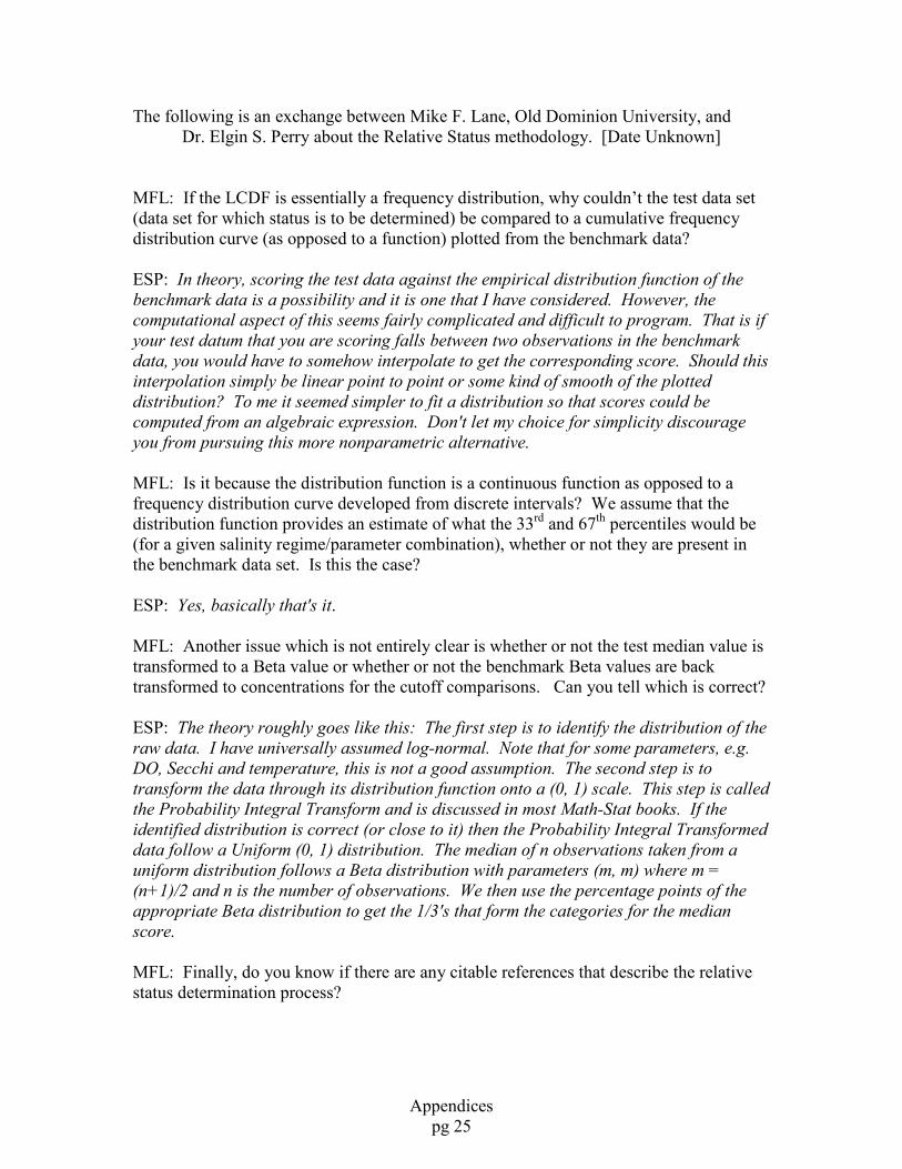
The following is an exchange between Mike F. Lane, Old Dominion University, and
Dr. Elgin S. Perry about the Relative Status methodology. [Date Unknown]
MFL: If the LCDF is essentially a frequency distribution, why couldn’t the test data set
(data set for which status is to be determined) be compared to a cumulative frequency
distribution curve (as opposed to a function) plotted from the benchmark data?
ESP: In theory, scoring the test data against the empirical distribution function of the
benchmark data is a possibility and it is one that I have considered. However, the
computational aspect of this seems fairly complicated and difficult to program. That is if
your test datum that you are scoring falls between two observations in the benchmark
data, you would have to somehow interpolate to get the corresponding score. Should this
interpolation simply be linear point to point or some kind of smooth of the plotted
distribution? To me it seemed simpler to fit a distribution so that scores could be
computed from an algebraic expression. Don't let my choice for simplicity discourage
you from pursuing this more nonparametric alternative.
MFL: Is it because the distribution function is a continuous function as opposed to a
frequency distribution curve developed from discrete intervals? We assume that the
distribution function provides an estimate of what the 33rd and 67
th percentiles would be
(for a given salinity regime/parameter combination), whether or not they are present in
the benchmark data set. Is this the case?
ESP: Yes, basically that's it.
MFL: Another issue which is not entirely clear is whether or not the test median value is
transformed to a Beta value or whether or not the benchmark Beta values are back
transformed to concentrations for the cutoff comparisons. Can you tell which is correct?
ESP: The theory roughly goes like this: The first step is to identify the distribution of the
raw data. I have universally assumed log-normal. Note that for some parameters, e.g.
DO, Secchi and temperature, this is not a good assumption. The second step is to
transform the data through its distribution function onto a (0, 1) scale. This step is called
the Probability Integral Transform and is discussed in most Math-Stat books. If the
identified distribution is correct (or close to it) then the Probability Integral Transformed
data follow a Uniform (0, 1) distribution. The median of n observations taken from a
uniform distribution follows a Beta distribution with parameters (m, m) where m =
(n+1)/2 and n is the number of observations. We then use the percentage points of the
appropriate Beta distribution to get the 1/3's that form the categories for the median
score.
MFL: Finally, do you know if there are any citable references that describe the relative
status determination process?

Appendices
pg 26
ESP: I don't know if there is a reference that chains these theorems together like this.
That may be my own creation, but I've not researched this enough to know. The
individual theorems are all in:
Roussas, George G. (1973), A First Course in Mathematical Statistics. Addison-Wesley, Reading, Mass.
MFL: Our current explanation of the process is provided below. Is it accurate? Also
take a look at the figure below and let us know if it accurate as well.
“Relative status scores are determined by comparing median values of the segment,
parameter and time period of interest against values derived from a benchmark data set
consisting of the first ten years of water quality data in Chesapeake Bay. A logistic
cumulative frequency distribution curve was developed for each parameter within each of
four salinity regimes: tidal freshwater, oligohaline, mesohaline and polyhaline using data
from the benchmark data set. The logistic cumulative frequency distribution curve was
used to generate a Uniform probability density distribution which ranged from 0 to 1 such
that higher values in the distribution represented poorer or less desirable water quality
conditions. Transformed median values from the test data are distributed according to a
Beta distribution and were assigned a score based on their location along the Beta density
distribution. If high values of a parameter are considered to be indicative of poor water
quality (nutrients, chlorophyll a, and suspended solids) then median values with a
corresponding Beta value greater than the 67th percentile of the Beta density distribution
(approximately) are classified as poor. Median values less than the 33rd percentile
(approximately) are classified as good and all values between these two cutoffs are
considered fair. If high values of a parameter are considered to be indicative of good
water quality (Secchi depth) then median values with a corresponding Beta value less
than the 33th percentile (approximately) are classified as poor. Median values greater
than the 67th percentile (approximately) are classified as good and all values between
these two cutoffs are considered fair. See the figure below for what we believe is the
status determination process.” [ESP edits in Italics and underlined]
ESP: The above is pretty close - here is my [version]:
“The status of each station is determined by comparison to a benchmark data set
comprised of all data for the years 1985-1990 collected by both Virginia and Maryland
programs.
Each station is rated as poor, fair, or good relative to the benchmark data. For each
salinity zone the ratings are obtained by the following steps:
1) For each parameter in the benchmark data set, a transformation is chosen that yields a
distribution that is symmetric and reasonably well approximated by the logistic
cumulative distribution function (CDF). In most cases, the logarithm transformation is
satisfactory.

Appendices
pg 27
2) A logistic CDF based on the mean and variance of each parameter of the benchmark
data set is used to perform a probability integral transform on all data in the most recent
3-year period. This results in data in the interval (0, 1) which follows a uniform
distribution (Roussas, 1973).
3) The 3-year median of this 0-1 data is computed as an indicator of status in the current
3-year period. The median of n observations taken from a uniform distribution follows a
Beta distribution with parameters (m, m) where m = (n+1)/2 and n is the number of
observations (Roussas, 1973).
4) Based on the Beta density, the distribution of 3-year medians from the benchmark
data is divided into thirds. If the median of the current 3- year period is in the upper
third (where upper is chosen as the end of the distribution that is ecologically desirable),
then the status rating is “good”, a median in the middle third is rated “fair”, and a median
in the lower third is rated “poor”.”
In most cases, serial dependence of the raw data resulted in greater than expected
variance in the Beta density of the medians. To adjust for this, the variance of the Beta
density is increased by a function of the ratio of among-station variance to within-station
variance.
ESP: I think [the figure below] works.

Appendices
pg 28

Appendices
pg 29
Appendix 4
Excerpt from
Assumptions and Procedures for Calculating
Water Quality Status and Trends
In Tidal Waters of the
Chesapeake Bay and its Tributaries
A cumulative history
Prepared for the Tidal Monitoring and Analysis Workgroup
(previously the Data Analysis Workgroup)
Chesapeake Bay Program
by
Elizabeth Ebersole, MD/DNR
Mike Lane, VA/Old Dominion University
Marcia Olson, NOAA Chesapeake Bay Office
Elgin Perry, Statistical Consultant
Bill Romano, MD/DNR
Updated January 2002

Appendices
pg 30
Introduction
The Chesapeake Bay Monitoring Program Analysis Methods were compiled at the direction of
the Tidal Monitoring Analysis Work Group (TMAW, formerly the Data Analysis Work Group–
DAWG) of the Monitoring Subcommittee. This document summarizes the data analysis methods
used by the Monitoring Program investigators to determine status (current condition) and trends
(overall increases or decreases over time). This document also describes the adjustments made
over time and as necessitated by the individual peculiarities associated with analyzing water
quality, living resource or benthic data.
Status
Status is a measure of current condition compared to some benchmark. For some water quality
and living resource parameters, reference levels such as restoration target levels or goals have
been established and the current condition of an area can be assessed with respect to that level.
Status assessment determines if current levels "meet," "fail," or are “borderline” with respect to
the target level. Because reference levels are not available for many parameters and because
there is some interest in how areas compare to others of similar type, efforts to develop a relative
measure of status have been ongoing. Relative status compares recent data for a specific
parameter at a particular station or segment to all stations and segments of the same salinity
regime in a benchmark dataset. Based on this comparison, the station or segment is given a
ranking of "good", "fair" or "poor" for the parameter in question. For most measures of status in
the TMAW analyses, using either reference or relative benchmarks, "recent" or "current" data are
those collected during the most recent three years.
Reference status – The number of water quality parameters and living resources that
have specific goals, target levels, or regulatory criteria is limited, but growing. Methods of
assessing status with respect to these levels are different, depending both on the parameter and
how the reference level is defined. For example, habitat requirements for submerged aquatic
vegetation (SAV) have been determined, and acceptable levels of five parameters critical to SAV
growth (light, DIN, DIP, chlorophyll, and suspended solids) established for the various salinity
zones during the SAV growing season. The requirements apply only to surface waters. Initially,
status was assessed by comparing the 3-year seasonal median values to the requirement value.
For example, the requirement for suspended solids is met if seasonal median concentrations are
at or below 15/mg/L. More recently, a more rigorous approach has been used in order to give
statistical confidence to the assessment. The Wilcoxon Signed Rank Test uses the individual
monthly values to determine if the location is signficantly (p<0.05) above or below the
requirement level or not significantly different (borderline).
Goals for dissolved oxygen (DO) have also been established. These apply to spring spawning
and summer seasons and set target levels specific to above- and below-pycnocline waters. The
goals and methods for assessing attainment are described in (ref). However, new DO criteria and
compliance measures currently being developed as part of the TMDL (Total Minimum Daily
Load) process will no doubt supercede thoe habitat restoration goals.
Appendices
pg 31
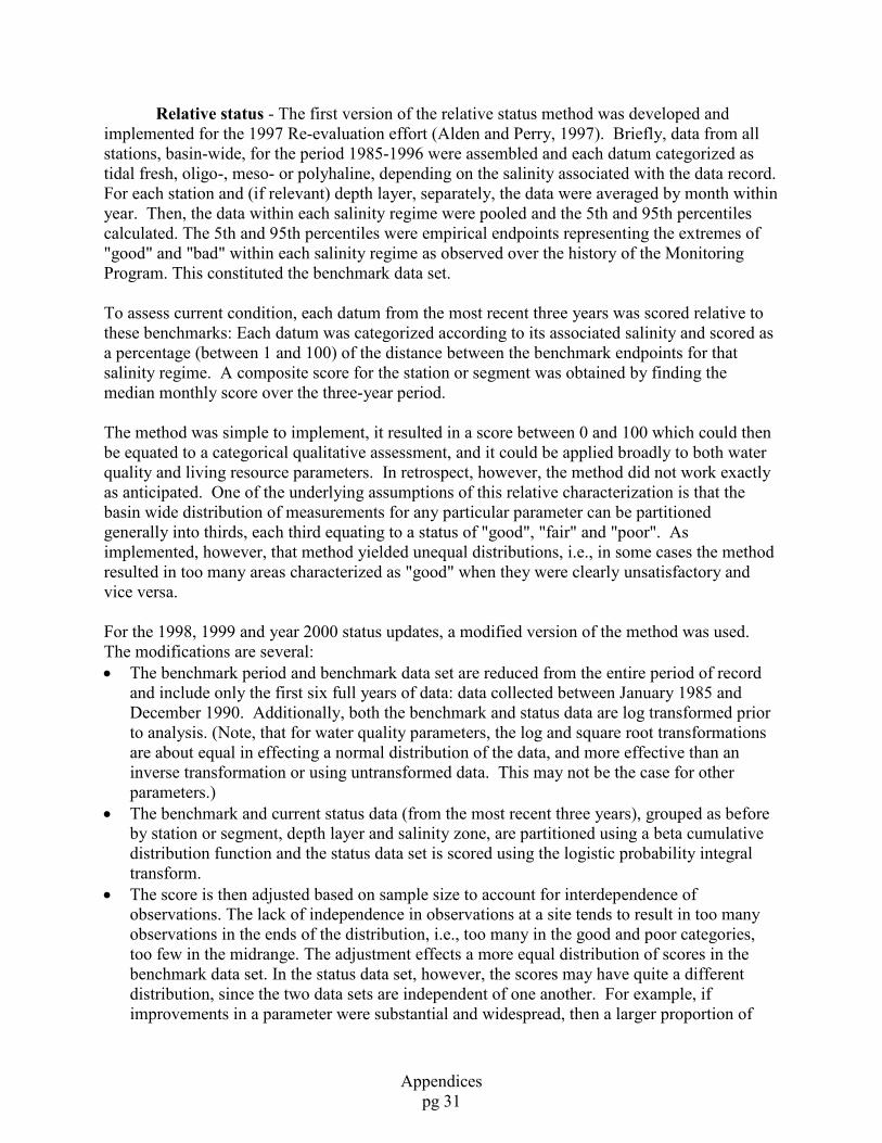
Relative status - The first version of the relative status method was developed and
implemented for the 1997 Re-evaluation effort (Alden and Perry, 1997). Briefly, data from all
stations, basin-wide, for the period 1985-1996 were assembled and each datum categorized as
tidal fresh, oligo-, meso- or polyhaline, depending on the salinity associated with the data record.
For each station and (if relevant) depth layer, separately, the data were averaged by month within
year. Then, the data within each salinity regime were pooled and the 5th and 95th percentiles
calculated. The 5th and 95th percentiles were empirical endpoints representing the extremes of
"good" and "bad" within each salinity regime as observed over the history of the Monitoring
Program. This constituted the benchmark data set.
To assess current condition, each datum from the most recent three years was scored relative to
these benchmarks: Each datum was categorized according to its associated salinity and scored as
a percentage (between 1 and 100) of the distance between the benchmark endpoints for that
salinity regime. A composite score for the station or segment was obtained by finding the
median monthly score over the three-year period.
The method was simple to implement, it resulted in a score between 0 and 100 which could then
be equated to a categorical qualitative assessment, and it could be applied broadly to both water
quality and living resource parameters. In retrospect, however, the method did not work exactly
as anticipated. One of the underlying assumptions of this relative characterization is that the
basin wide distribution of measurements for any particular parameter can be partitioned
generally into thirds, each third equating to a status of "good", "fair" and "poor". As
implemented, however, that method yielded unequal distributions, i.e., in some cases the method
resulted in too many areas characterized as "good" when they were clearly unsatisfactory and
vice versa.
For the 1998, 1999 and year 2000 status updates, a modified version of the method was used.
The modifications are several:
• The benchmark period and benchmark data set are reduced from the entire period of record
and include only the first six full years of data: data collected between January 1985 and
December 1990. Additionally, both the benchmark and status data are log transformed prior
to analysis. (Note, that for water quality parameters, the log and square root transformations
are about equal in effecting a normal distribution of the data, and more effective than an
inverse transformation or using untransformed data. This may not be the case for other
parameters.)
• The benchmark and current status data (from the most recent three years), grouped as before
by station or segment, depth layer and salinity zone, are partitioned using a beta cumulative
distribution function and the status data set is scored using the logistic probability integral
transform.
• The score is then adjusted based on sample size to account for interdependence of
observations. The lack of independence in observations at a site tends to result in too many
observations in the ends of the distribution, i.e., too many in the good and poor categories,
too few in the midrange. The adjustment effects a more equal distribution of scores in the
benchmark data set. In the status data set, however, the scores may have quite a different
distribution, since the two data sets are independent of one another. For example, if
improvements in a parameter were substantial and widespread, then a larger proportion of

Appendices
pg 32
recent data would be "fair" or "good" relative to the benchmark period and a smaller
proportion would be "poor."
References
Alden, R. W. III, and E. S. Perry 1997. Presenting Measurements of Status. A “white paper”
written for and presented to the Chesapeake Bay Program Data Analysis Workgroup; 15 pp.

Appendices
pg 33
Maryland and Virginia Mainstem and Tidal Tributaries
A Little History
Over the years of the Monitoring Program, analytical methods have changed or been modified.
Some of the changes have been due to changes in parameters and laboratory techniques, others
have been due to new statistical techniques and/or new thinking; still other changes have
followed because of technological advances in data management and communications. In the
wake of such change, comparability and consistency issues have been and will continue to be
challenges to the workgroup.
Historically, responsibility for water quality status and trend analyses was divided among the
primary Monitoring Program partners, albeit under the auspices and guidance of the analytical
workgroup. Maryland state staff or grantees performed the analyses for Maryland tidal
tributaries; Virginia commonwealth staff or grantees performed the analyses for Virginia tidal
tributaries; and USEPA Bay Program staff performed the analyses for the mainstem Bay.
Although analyses were performed by different entities, the same methods, conceptually, were
used and modified as necessary to conform to the individual sampling programs. With the
advent of the CIMS data base and universal access to data through the web, it was thought that
cost efficiencies and consistency could be gained by centralizing the analyses. In year 2000,
preliminary data preparation was performed by the separate partners, but the status and trend
analyses (covering data through 1999) for the Bay and tributaries were all done by Bay Program
staff. Although benefits were derived from that exercise, the responsibility for review and
interpretation of the results still resided, rightly, with the separate partners, and the back and
forth of data sets and results proved cumbersome and time-consuming. In 2001, Maryland staff
performed the analyses for the Maryland tributaries and Bay Program staff performed the
analyses for the mainstem and Virginia tributaries. Both groups used the same computer
programs for all aspects of analysis and reporting.
Note: in the following sections, terms such as “1997 update” refer to analyses of data records
that have been updated with data collected in the year named, e.g., 1997. The analyses were
actually performed and the results reported in the following year.
Parameters
The core parameters for which status and trend analyses are conducted each year are listed
below.
Four nutrient parameters:
• total nitrogen (TN);
• dissolved inorganic nitrogen (DIN);
• total phosphorus (TP); and
• dissolved inorganic phosphorus (DIP).
Eight additional parameters:

Appendices
pg 34
• total suspended solids (TSS);
• active chlorophyll a (CHLA), as a response indicator of nutrient enrichment and habitat
quality;
• bottom dissolved oxygen (DO), as a response indicator of nutrient enrichment and habitat
quality;
• Secchi depth (SECCHI), as a measure of water clarity;
• "percent light at the leaf (PLL)," a calculated estimate of light reaching submerged aquatic
vegetation (SAV) at various depths. PLL is derived from the measurements of DIN, DIP and
TSS. For this update, PLL at 0.5 m and at 1m were analyzed.
• KD, a measure of light penetration; and
• salinity and
• water temperature.
Similar analyses for additional parameters may be available as well: e.g., particulate phosphorus
(PP), nitrite/nitrate (NO23), ammonia (NH4), silicate (SI) and carbon compounds (e.g. PC) ; also
nutrient ratios, such as TN:TP and DIN:DIP.
Flow-adjusted trend analyses have been conducted only on the four nutrient parameters TN,
DIN, TP, and DIP, and on TSS, CHLA and bottom DO. The most recent flow-adjusted trends
for water quality are for the 1985-1998 period. The flow-adjustment methodology is currently
under review.
Spatial and Temporal Scales
Water samples for laboratory analysis of nutrients, chlorophyll and suspended solids are
collected at surface and bottom and at 1 m above and 1 m below the pycnocline, if one exists.
For status and trend analyses, where both surface and above-pycnocline samples are collected,
measurements are averaged, resulting in one value for the surface-mixed layer. Likewise, where
both bottom and below-pycnocline samples are collected, measurements are averaged, resulting
in one value for the bottom-mixed layer. Trend analyses are done separately for surface-mixed
and bottom-mixed layers. In the Virginia tributaries, chlorophyll is measured only at the surface
and in some regions, the number of missing values for other parameters preclude analysis of
bottom measurements.
[Note: in 1997 and 1998, status assessments for surface chlorophyll used only surface
measurements, even when above-pycnocline measurements were available. Chlorophyll is
measured only in surface waters in the Virginia tributaries, and this was intended to equalize data
handling among segments. In subsequent years, it was decided to use all available data and treat
as indicated above. ]
Water temperature, salinity and dissolved oxygen are measured in-situ at 1- to 2-m intervals
through the water column. In the case of dissolved oxygen, only bottom concentrations are
analyzed for status and trends. For salinity and water temperature, only surface and bottom
measurements are analyzed for trends; status is not evaluated for these two parameters.

Appendices
pg 35
Annual routine status and trend analyses are conducted using water quality data collected from
the Chesapeake Bay mainstem and tidal tributaries from January 1985 (or from the beginning
date if the program began later) through December of the most recent year. The core seasonal
analyses include:
• the annual season or calendar year (months 1-12);
• the SAV growing season (months 4-10 in tidal fresh, oligohaline and mesohaline regions,
and months 3-5 and 9-11 in polyhaline regions);
• spring (months 3-5 in polyhaline regions and 4-6 in other salinity zones); and
• summer, which is defined differently for different parameters. For dissolved oxygen,
summer includes months 6-9; for chlorophyll a, summer includes months 7-9. For most
parameters, analyses are done for all season definitions.
The flow-adjusted data are analyzed for trend only over the annual season (months 1-12). Flow-
adjusted data are not assessed for status.
For a regional picture of status and trends, stations are aggregated for analysis into segments.
Prior to 1997, by-segment analyses used the original CBP segmentation scheme. The
segmentation was modified for the1997 Reevaluation Effort to reflect more closely the salinity
conditions of the evaluation period, i.e., 1985 and subsequent years. Status and trend analyses
for the 1997 update used this station aggregation. In 1998, the segmentation scheme was further
modified slightly. This scheme is the basis for 1998 to present by-segment analyses.
Documentation of the chronology and definition of the several schemes (Olson, 2000) is
available on line in the TMAW Source Library.
Status Calculations
As described in the introduction (page 1)
Trend Analysis and Flow-Adjusting Procedures
As described in the introduction (page 1), with the following additional details.
Flow adjustment in the mainstem Bay – The mainstem Bay receives discharges from
large and small tributaries up and down its length and it is difficult to remove the effects of flow
for main Bay stations in the same way as done for the tributary stations. At the request of the
data analysis workgroup, Ray Alden and colleagues developed a flow-adjustment for the main
Bay in time for the 1997 trend update. Like the flow adjustment procedure for the tributaries,
this method is also currently under review. The flow-adjusted analysis was not performed for the
2000 update.
The “adjustment” for the mainstem is, in fact, segment-specific regression models that include a
flow factor as well as various pre-selected month, depth, salinity and/or water temperature
factors, if they added significantly to the model fit. The input value for daily flow is the sum of
the daily flows of the major tributaries discharging to the Bay at or north of the segment being
analyzed. Similar to the procedure applied in the tributaries, the procedure finds the best
predictive flow variable among several and removes the variance associated with flow and

Appendices
pg 36
associated variables by subtracting the least squares prediction from the observed response.
Copies of these programs are archived online in the TMAW Source Library.
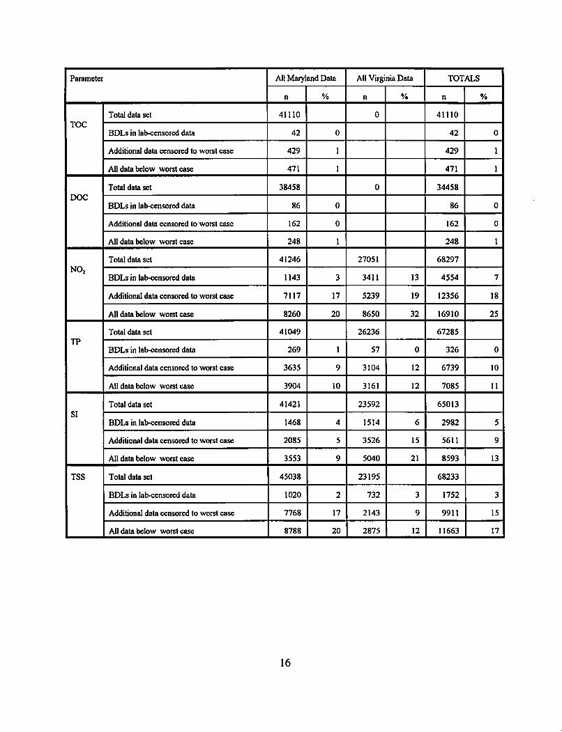
Decision Rules for Reporting Trends With Observations Below Detection Limit - In
the CBP water quality monitoring database, parameters whose levels are below the detection
limit of the analytical method are assigned the value of the detection limit. Over the history of
the Monitoring Program, many of the laboratory analytical techniques have changed or improved
and lowered their limit of detection. An artifact of this advance is that the lower values of the
BDL measurements later in the data record may be falsely detected as a downward trend. To
avoid this, water quality values are censored to the highest detection limit of the analysis period
as part of the data handling prior to analysis. Censoring is based on the detection-limit history of
each station for the individual station analyses. For segment analyses, however, where stations
within a single segment are monitored by different organizations and have different detection
limits, the censoring level is the highest detection limit of the stations in the segment. After
censoring, all censored data are set to one-half the detection limit value.
Data sets having large numbers of values below detection limit (BDLs) may create statistical
problems for trend analyses. The Seasonal Kendall test for trend, and similar sign tests such as
the Van Belle and Hughes test, adjust variance estimates upward for ties in magnitude. Since
BDL values in the raw data set produce such ties, trend analyses of data sets with high
percentages of BDLs will be based upon greater variances than those without BDLs, all else
being equal. Thus, the power of the trend analyses for the data sets with BDLs will be reduced
compared to those without detection limit censoring.
There is an additional wrinkle to flow-adjusted data. When a data set with BDL values is flow-
adjusted by the procedures previously described, many ties in magnitude disappear, since each
datum is adjusted based upon the flow measurement from the day of collection. As a result, the
trend analyses conducted after flow adjustment will, in all probability, have fewer ties in
magnitude, lower variances and an artificial increase in power compared to the trend analysis
based upon the observed data. This increase in power is an artifact of the flow adjusting process
and is not based on changes in the magnitude of trends that are due to flow.
The DAWG guidelines for reporting Seasonal Kendall trend test results, with respect to BDLs,
have changed over the years. For the 1985-1997, -1998 and –1999 updates, the following rules
applied:
• If a significant trend result is obtained and more than 5% of the data are below the worst case
detection limit, then report the direction of trend, but not the magnitude (percent change).
• If more than 20% of the data is censored, then report neither the direction nor magnitude of
trend.
• If results are significant only for flow adjusted data and more than 5% of which are BDL,
confirm the results through the use of a Tobit analysis procedure (Tobin,1958). Tobit
analysis is a regression-based procedure that is designed to handle left censoring such as
occurs with lower detection limits.
For the 1985-2000 trend updates, DAWG adopted different decision rules:

Appendices
pg 37
• If the percentage of BDL observations is 15 or less, report the Seasonal Kendall trend test
p-value and direction as well as the Sen Slope estimator of the magnitude of the trend (e.g.,
35 %).
• If the percentage of BDL observations is greater than 15 and less than or equal to 35, report
the Seasonal Kendall trend test p-value and direction, but do not report the Sen Slope
estimator of trend magnitude.
• If the percentage of BDL observations is greater than 35 and less than or equal to 50 and the
Seasonal Kendall trend test p-value indicates a significant trend, report the Seasonal Kendall
trend test p-value and direction, but do not report the Sen Slope estimator of trend magnitude.
• If the percentage of BDL observations is greater than 35 and less than or equal to 50 and the
Seasonal Kendall trend test p-value does not indicate a significant trend, report nothing,
noting that there are too many observations below the detection limit to determine the
presence or absence of trend.
• If the percentage of BDL observations is greater than 50, report nothing, noting that too
many observations were below the detection limit to determine the presence or absence of
trend.
Rationale - The rationale for these rules is based on findings demonstrated by simulation
analysis for the Seasonal Kendall test and Sen slope estimator (Alden, Perry and Lane, 2000) and
is briefly summarized here: 1) The false positive rate of the Seasonal Kendall test does not seem
to be affected by the level of censoring of the data; 2) The power of the Seasonal Kendall test
begins noticeably to decline when censoring exceeds 35 %; 3) The Sen slope estimator begins
noticeably to exhibit bias when censoring exceeds 15%. At levels of censoring of 15% or less,
both the Seasonal Kendall test results and the Sen slope estimator are reliable and should be
reported. At levels of censoring greater than 15%, the Sen slope estimator should not be
reported because it becomes biased. The Seasonal Kendall test retains a robust type I error rate
and a flat power response up to 35% censoring and thus should be reported up to that level. If
the Seasonal Kendall test produces a significant result when the level of censoring exceeds 35%,
one may infer that this result is obtained in spite of the loss of power and therefore is a valid
result and should be reported. If the Seasonal Kendall procedure fails to produce a significant
result when censoring is in the 35% to 50% interval, this failure may have resulted from a loss of
power and should be reported as a non-significant result, which carries the implication that the
trend is below the level that we have power to detect with an uncensored data set. While the
Seasonal Kendall procedure continues to exhibit the nominal type I error rate for levels of
censoring that are greater than 50%, and thus significant results for these high levels of censoring
might be judged reliable, the risk that the uncensored data are unduly influenced by a large scale
stochastic event (e.g. drought, hurricane, etc.) becomes large and these results should not be
reported.
Determining percent BDL – This aspect of the analytical methodology seemed self-
evident at first and was not formally discussed or delineated in detail. The several reporting
entities used the same censoring procedure for each datum (i.e., setting values lower than the
highest theoretical detection limit to one-half the detection limit value), but otherwise each “did
their own thing.” For the 1998 and 1999 updates, the workgroup defined a more detailed
procedure. It was modified somewhat for the 2000 update.

Appendices
pg 38
• Flag and censor each value below the highest detection limit over the trend period.
For parameters that are directly measured during the whole time period, the detection limit is
simply the highest measured detection limit used for that parameter over the time period. For
example, the highest detection limit for orthophosphate (PO4) at stations in Maryland minor
tributaries between 1985 and the present is 0.01 mg/L. This was the detection limit at the
analytical laboratory from 1985 to May 31, 1986.
For calculated parameters, i.e., parameters derived by addition or subtraction from directly
measured parameters, the theoretical detection limit is the sum of the detection limits of the
constituent parameters. The highest theoretical detection limit, then, is the highest of such
sums over the trend period. For example, total nitrogen (TN) is obtained from
TKNW+NO23 and/or from PN + TDN, depending on which constituents are measured.
Both methods have been used over the history of most stations in the Monitoring Program.
For example, at mainstem Bay stations, TN was obtained by the first method from the
beginning until October 1987, and by the second thereafter. At a station in the lower Bay
sampled, say, by VIMS, the highest detection limits for TKNW and NO23 at any given time
in those years sum to 0.11 mg/L; the highest for PN+TDN is 0.10. Thus, the data are
censored to one half of the higher of the two methods, to 0.11/2 mg/L.
• Censor monthly mean values. The Seasonal Kendall trend test is performed on monthly
mean values for separate depth layers of various definition, e.g., surface, surface-mixed,
lower-mixed, and bottom layers. In the first version of the procedure, the monthly value for
each layer was considered BDL if the number of censored (flagged) measurements was >=
50% of the individual sample values. For example, 2 sampling events at a deep water station
in July yields 4 total values in the mean for the surface-mixed layer: 1sample each from
surface and above-pycnocline layers, times 2 events. If 2 or more of those 4 values are BDL,
then the monthly value was considered BDL in this version.
This decision rule was modified in the 2000 update. Since the BDL issue is actually an issue
of “ties” between months in the Seasonal Kendall test, the possibility of a tie due to
censoring is eliminated if any one of the values in the monthly mean is not BDL. Thus, in
the modified version, a monthly mean value is flagged as BDL only if all of the values in the
mean are BDL.
• Compute BDL percentage based on station/segment-layer-season group. The trends are
calculated either by segment or by station for a given layer for various defined seasonal
groupings. The percent BDL for a parameter is the number of BDL monthly mean values
divided by the total number of monthly mean values in the station/segment-layer-season
group of values for that parameter. The results, with respect to BDLs, are reported or
suppressed based on the decision rules given above.
Reporting Rules for Non-homogeneous Trend Results - The procedure by van Belle and
Hughes (1984) is used to test for homogeneity of trend among months to see if the trend is
consistent across months within seasons and across stations within segments. Homogeneity
within seasons is tested and considered significant at p<= 0.01. If trends among months within

Appendices
pg 39
seasons for a given station are not homogeneous, then the analyst reviews the data and uses
professional judgment to determine if the overall annual trend is considered valid and can be
reported with confidence. The default rule is to report the trend. If the analyst finds reason for
no confidence, then "no trend" is reported.
Related Information
For details on water quality field sampling or laboratory analysis methods in Maryland, see
http://www.dnr.state.md.us/bay/tribstrat/status_trends methods.html or contact Elizabeth L.
Ebersole, Tidewater Ecosystem Assessment, Maryland Department of Natural Resources, 580
Taylor Avenue, Annapolis, MD 21401, [email protected]. In Virginia, contact F. A.
Hoffman, VA Dept. of Environmental Quality, P.O. Box 10009, Richmond, VA 23240,
References
Alden, R. W., E. S. Perry, and M. F. Lane. 2000. A Comparison of Analytical Techniques for
Determining Trends in Chesapeake Bay Water Quality Monitoring Program Data. AMRL
Technical Report # 3114. Applied Marine Research Laboratory, Norfolk, Va.
Olson, M. M. 2000. Analytical Segmentation Scheme for the 1997 Re-evaluation and Beyond,
prepared for the USEPA Chesapeake Bay Program Office by the Monitoring Subcommittee Data
Analysis Workgroup.
Tobin, J. 1958. Estimation of Relationships for Limited Dependent Variables. Econometrica.
26:24-36.