relatorio final de projecto - estudo geral: home report 5th year graduation in biomedical...
TRANSCRIPT
Departamento de Física
Universidade de Coimbra
Cardioaccelerometery
The assessment of Pulse Wave Velocity using Accelerometers
Project Report 5th year
Graduation in Biomedical Engineering
Helena Catarina de Bastos Marques Pereira
Setembro de 2007

Faculdade de Ciências e Tecnologia da Universidade de Coimbra
Faculdade de Medicina da Universidade de Coimbra
This report is made in fulfillment of the
requirements of Project, a discipline of the 5th
year of the Biomedical Engineering graduation.
Supervisors
Prof. Dr. Carlos M. Correia
Prof. Dr. Luís Requicha Ferreira
Physics Department FCTUC
External
Supervisor
João Maldonado, MD
Instituto de Investigação e Formação Cardiovascular

iii

iv
“…Pedras no caminho?
Guardo todas, um dia vou construir um castelo…”

v

vi
ABSTRACT
In the past recent years, great emphasis has been placed on the role of arterial stiffness in
the development of cardiovascular diseases, recognized as the leading cause of death in the
world. This hemodynamic parameter, generally associated to age and blood pressure increase,
can be assessed by the measurement of the pulse wave velocity (PWV), i.e., the velocity at which
the pressure wave propagates along an artery. Although PWV measurement is accepted as the
most simple, non-invasive, robust and reproducible method to determine arterial stiffness over
the carotid-femoral region, the devices available in the market for this purpose are extremely
expensive.
This research project aims at developing alternative instrumental methods for the aortic
PWV’s hemodynamic characterization and, at a later stage, a software application for acquisition
and interpretation of this information. The proposed instruments are constituted by one
accelerometric probe and a multisensor acquisition module, which includes classic electrodes of
electrocardiography, piezoelectric (PZ) transducers and, foreseen, one pressure sensor.
Up to now, in its research usage, it has proved effective in the prolonged follow up of
hypertensive patients without and with drug treatment, allowing the study of correlations
between the different types of signals. A valuable contribution to this study has been given by
the bench models developed in laboratory for the ADXL203 accelerometer calibration and
pulsatory system simulation.
This report describes not only the aspects related with the overall instrument
architecture, the successive developed versions and the results obtained, under medical control,
for each of the input signals, but also the calibration and pulsatory models and respective
results.
Keywords: Cardiovascular Diseases, Aortic Stiffness, Pulse Wave Velocity, Accelerometer based
Probe, Multisensor Acquisition Module, Clinical Research Tests.
vii
RESUMO
Nos últimos anos, tem sido dada grande ênfase ao papel da rigidez arterial no
desenvolvimento de doenças cardiovasculares, reconhecidas como a principal causa de morte
mundial. Este parâmetro hemodinâmico, associado normalmente ao aumento da idade e da
pressão arterial, pode ser avaliado pela medição da velocidade de onda de pulso (VOP), ou seja, a
velocidade com que a onda de pressão se propaga ao longo de uma artéria. Embora a medição da
VOP seja aceite como o método mais simples, não-invasivo, robusto e reprodutível para determinar
a rigidez arterial ao longo da região carótida-femoral, os equipamentos disponíveis no mercado
para este efeito são extremamente dispendiosos.
Este projecto de investigação pretende desenvolver métodos instrumentais alternativos para
a caracterização hemodinâmica da VOP aórtica e, numa fase mais avançada, uma aplicação
informática que permita a aquisição e a interpretação dessa informação. Os instrumentos
propostos são constituídos por uma ponta de prova acelerométrica e um módulo de aquisição
multisensor, que incorpora eléctrodos clássicos de electrocardiografia, transdutores piezoeléctricos
e, como previsão, um sensor de pressão.
Até agora, o seu uso em testes clínicos, provou ser eficaz no seguimento prolongado de
pacientes hipertensivos sem e com tratamento de fármacos, permitindo o estudo de correlações
entre os diferentes tipos de sinais. Para este estudo contribuiram ainda os modelos de bancada
desenvolvidos em laboratório, com vista à calibração do acelerómetro ADXL203 e à simulação de
um sistema pulsatório.
Neste relatório são descritos não só os aspectos ligados à arquitectura do instrumento, as
sucessivas versões desenvolvidas e os resultados obtidos, sob supervisão médica, para cada um dos
canais de informação, mas também, os modelos de calibração e pulsatório e, respectivos resultados.
Palavras-chave: Doenças Cardiovasculares, Rigidez Arterial, Velocidade de Onda de Pulso, Ponta
de Prova Acelerométrica, Módulo de Aquisição Multisensor, Testes Clínicos.

viii

ix
ACKNOWLEDGEMENTS
This academic project has been a great personal learning experience and I would like to
thank everyone who helped me throughout this year.
First and foremost, I am very grateful to my supervisors, Prof. Dr. Carlos Correia and
Prof. Dr. Requicha Ferreira by their continuous guidance, support, assistance and friendship.
Prof. Dr. Carlos Correia is the author of this project idea and was a great counsellor throughout
my graduation. Prof. Dr. Requicha Ferreira, due to his technical expertise and creative mind, was
essential in this project fulfilment.
Special thanks go to the other member of this team: Dr. João Maldonado, who supervised
all clinic tests and without his medical knowledge and helpful discussions this work would not
have been possible. Thanks to the staff that work at Instituto de Investigação e Formação
Cardiovascular for their invaluable collaboration and sympathy.
The Centro de Electrónica e Instrumentação has a great environment and I must thank
all for the kindness and availability, not forgetting for sure my work colleagues, Ana and Edite,
for their group effort.
I would like to express my gratitude also to Engº Augusto, who gave an important
assistance, as far as the mechanical part of this project is concerned.
My deepest thanks go to my parents, brothers and friends for their constant support and
encouragement. They have always allowed me to keep my mental and physical shape
throughout my studies, particularly one person, Paulo, who always has been there.

x
xi
CONTENTS
Abstract ................................................................................................................................................. vi
Resumo ................................................................................................................................................. vii
Acknowledgments .......................................................................................................................... ix
List of Figures .................................................................................................................................... xiii
List of Tables ...................................................................................................................................... xv
1. Introduction .................................................................................... 1
1.1 Motivation ..................................................................................................................................... 1 1.2 Objectives ....................................................................................................................................... 2 1.3 Hemodynamic project team ................................................................................................... 3 1.4 Overview of the report ............................................................................................................. 4
2. Theoretical Background ............................................................. 4
2.1 Arterial Stiffness and Pulse Wave Velocity ...................................................................... 4 2.1.1 General Concepts ........................................................................................................... 4 2.1.2 PWV Measurement ....................................................................................................... 5 2.1.2.1 State of the art ................................................................................................. 6
2.2 Accelerometric Sensors ........................................................................................................... 8 2.2.1 Introduction ..................................................................................................................... 8 2.2.2 General Concepts ........................................................................................................... 8
2.3 Electrocardiography .................................................................................................................. 11 2.3.1 Introduction ..................................................................................................................... 11
2.3.2 Components of the ECG ...................................................................................... 12 2.3.3 Instrumentation Requirements ............................................................................... 13
3. Process Methodology .................................................................... 17
3.1 Introduction .................................................................................................................................. 17 3.2. Measurement System Architecture .................................................................................... 17 3.3 Clinical Trials ............................................................................................................................... 19
3.3.1 Data Acquisition ............................................................................................................. 19 3.2.2 Data Processing .............................................................................................................. 19
3.4 Discussion ...................................................................................................................................... 21
4. Measurement Probes .................................................................... 23
4.1 Introduction .................................................................................................................................. 23

xii
4.2 Spring-Loaded Probe ............................................................................................................... 24 4.3 Differential Probe ....................................................................................................................... 25 4.4 Hybrid Probe ................................................................................................................................ 27
5. Acquisition Modules ...................................................................... 29
5.1 Introduction .................................................................................................................................. 29 5.2 Module A ........................................................................................................................................ 29 5.3 Module B ........................................................................................................................................ 30 5.4 Module C ......................................................................................................................................... 31 5.5 Module D ........................................................................................................................................ 32 5.6 Module E ......................................................................................................................................... 33
6. Accelerometer Calibration .......................................................... 34
6.1 Introduction .................................................................................................................................. 34 6.1.1 Slider Crank Mechanism ............................................................................................. 34
6.2 Methods ……. ................................................................................................................................. 36 6.2.1 Experimental Configuration …… ............................................................................. 36 6.2.2 Experimental Measurements .................................................................................... 37
6.3 Results and Discussion ............................................................................................................. 37 6.3.1 Experience A ................................................................................................................... 37 6.3.2 Experience B ................................................................................................................... 38
6.4 Conclusions ................................................................................................................................... 40
7. Pulsatory model ............................................................................. 42
7.1 Bench Model Set-up ................................................................................................................... 42 7.2 Results ............................................................................................................................................. 43 7.3 Data Processing ........................................................................................................................... 43
8. Clinical Research Tests ................................................................ 46
8.1 CTs Procedures ............................................................................................................................ 46 8.2 Data Pre-Processing .................................................................................................................. 47
9. Conclusions and future work ..................................................... 51
9.1 Conclusions ............................................................................................................................. 51 9.2 Future Work .......................................................................................................................... 52
Appendices ............................................................................................ 53
Appendix A ..................................................................................................................................... 53 Appendix B ..................................................................................................................................... 57

xiii
LIST OF FIGURES
Figure 1 Measurement of PWV with the foot-to foot method.. ...................................................................... 6
Figure 2 Complior®. ........................................................................................................................................................ 6
Figure 3 Sphymocor® .................................................................................................................................................... 6
Figure 4 The basic spring mass system accelerometer . .................................................................................. 9
Figure 5 Flip Calibration ............................................................................................................................................. 10
Figure 6 Form of a normal ECG signal .................................................................................................................. 12
Figure 7 Cardiac Cycle Diagram. .............................................................................................................................. 12
Figure 8 Heart’s electrical activity .......................................................................................................................... 13
Figure 9 Typical single-channel electrocardiograph.. .................................................................................... 15
Figure 10 General measurement system architecture................................................................................... 18
Figure 11 NI USB-6008©. .......................................................................................................................................... 18
Figure 12 Developed Instrument. .......................................................................................................................... 19
Figure 13 Original Signals of a young and healthy subject, obtained with the accelerometer
based instrument and visualized in Matlab®. .................................................................................................... 20
Figure 14 Overlap of eight selected peaks and mean of these overlapped peaks. ............................. 21
Figure 15 Pulse wave Contour in some arteries. .............................................................................................. 22
Figure 16 SLP .................................................................................................................................................................. 24
Figure 17 Schematic of the forces applied on the SLP during data acquisition. .................................. 25
Figure 18 DP. ................................................................................................................................................................... 26
Figure 19 Hybrid Probe. ............................................................................................................................................ 28
Figure 21 DAQ Module B. ........................................................................................................................................... 30
Figure 22 Block Diagram of the linear power supply design. ..................................................................... 31
Figure 23 DAQ Module C. ........................................................................................................................................... 32
Figure 24 DAQ Module D. ........................................................................................................................................... 32
Figure 25 DAQ Module E. ........................................................................................................................................... 33
Figure 26 Crank Mechanism. .................................................................................................................................... 35
Figure 27 Graphic representation of the piston movement (blue) and MHS (red). .......................... 36
Figure 28 Experimental set-up of accelerometer calibration. .................................................................... 36
Figure 29 Data Pre Processing ................................................................................................................................ 39
Figure 30 Accelerometer’s Curve Calibration ................................................................................................... 40
xiv
Figure 31 Set-up of the developed bench model. ............................................................................................. 42
Figure 32 Accelerometric, PZ and pressure signals acquired in the pulsatory model..... ................ 44
Figure 33 Accelerometric and Double Differentiate PZ Signals ................................................................. 45
Figure 34 Signals acquired by the SLP/Module B in one patient. ............................................................. 47
Figure 35 Signals acquired by the SLP/Module C in one patient. ............................................................. 48
Figure 36 Signals acquired by the DP/Module D in one patient. ............................................................... 49
Figure 37 Functions of a piezoelectric sensor. .................................................................................................. 53
Figure 38 The Heart. .................................................................................................................................................... 54
Figure 39 Location of the precordial leads. ........................................................................................................ 55
Figure 40 Location of the electrodes in the Standard Limb Leads and Augmented Limb leads. . 55
Figure 41 ECG components: waves, segments and intervals. ..................................................................... 56
Figure 42 Measurement probe’s circuit schematic. ........................................................................................ 57
Figure 43 PZ Single Channel of DAQ Module B ................................................................................................. 57
Figure 44 PZ channel of DAQ Module C ................................................................................................................ 58
Figure 45 SPL Electronic Circuit Schematic. ...................................................................................................... 59
Figure 46 HP Electronic Circuit Schematic. ........................................................................................................ 60
Figure 47 Electrocardiograph Electronic Circuit Schematic. ...................................................................... 61
xv
LIST OF TABLES
Table 1 Team members of the project ‘Hemodynamic Parameters - New Instrumentation and
Methodologies’ and its contributions. ....................................................................................................................... 2
Table 2 Clinical conditions associated with increased arterial stiffness.. ................................................. 5
Table 3 Types of ECG leads. ....................................................................................................................................... 11
Table 4 Some NI USB-6008 Specifications . ........................................................................................................ 18
Table 5 Summary of the developed modules and its main features......................................................... 33
Table 6 Comparison between piston motion and SMH equations ........................................................... 35
Table 7 Amplitude, peak voltage and peak acceleration values ................................................................. 39
Table 8 Acquisition types performed with the various probes/modules. ............................................. 46

xvi
1
CHAPTER 1
INTRODUCTION
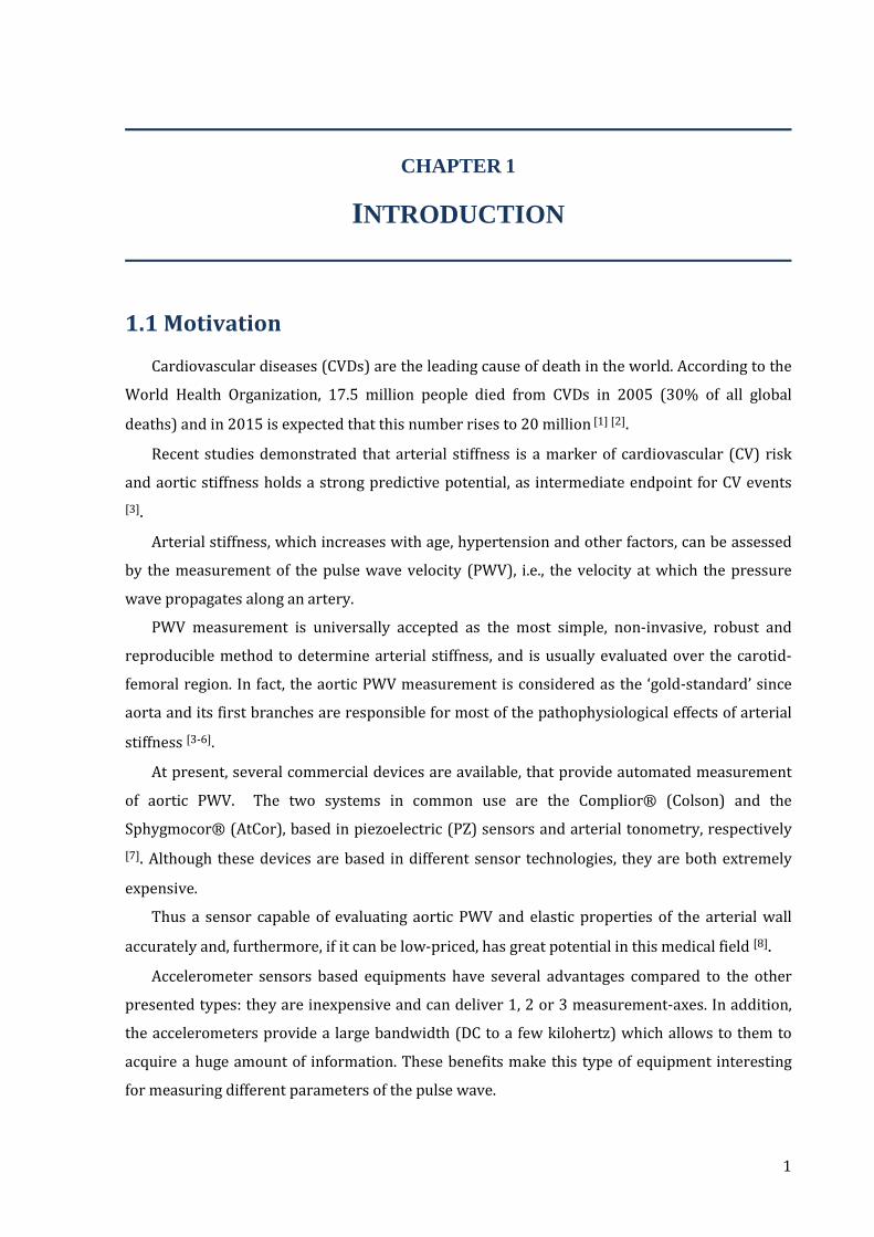
1.1 Motivation
Cardiovascular diseases (CVDs) are the leading cause of death in the world. According to the
World Health Organization, 17.5 million people died from CVDs in 2005 (30% of all global
deaths) and in 2015 is expected that this number rises to 20 million [1] [2].
Recent studies demonstrated that arterial stiffness is a marker of cardiovascular (CV) risk
and aortic stiffness holds a strong predictive potential, as intermediate endpoint for CV events
[3].
Arterial stiffness, which increases with age, hypertension and other factors, can be assessed
by the measurement of the pulse wave velocity (PWV), i.e., the velocity at which the pressure
wave propagates along an artery.
PWV measurement is universally accepted as the most simple, non-invasive, robust and
reproducible method to determine arterial stiffness, and is usually evaluated over the carotid-
femoral region. In fact, the aortic PWV measurement is considered as the ‘gold-standard’ since
aorta and its first branches are responsible for most of the pathophysiological effects of arterial
stiffness [3-6].
At present, several commercial devices are available, that provide automated measurement
of aortic PWV. The two systems in common use are the Complior® (Colson) and the
Sphygmocor® (AtCor), based in piezoelectric (PZ) sensors and arterial tonometry, respectively
[7]. Although these devices are based in different sensor technologies, they are both extremely
expensive.
Thus a sensor capable of evaluating aortic PWV and elastic properties of the arterial wall
accurately and, furthermore, if it can be low-priced, has great potential in this medical field [8].
Accelerometer sensors based equipments have several advantages compared to the other
presented types: they are inexpensive and can deliver 1, 2 or 3 measurement-axes. In addition,
the accelerometers provide a large bandwidth (DC to a few kilohertz) which allows to them to
acquire a huge amount of information. These benefits make this type of equipment interesting
for measuring different parameters of the pulse wave.

CARDIOACCELEROMETERY CHAPTER 1: INTRODUCTION
2
1.2 Objectives
The objectives of this project are to develop alternative instrumental methods, based in
accelerometery, for the PWV’s hemodynamic characterization and, at a later stage, also a
software application for acquisition and interpretation of this information. Both the developed
instrumental prototypes and the application must be conceived for use by staff technicians in a
clinical environment.
1.3 Hemodynamic project team
This project was carried out in the Centro de Electrónica e Instrumentação da
Universidade de Coimbra (CEI) in the framework of a partnership with Instituto de Investigação
e Formação Cardiovascular (IIFC). It is a part of the research project ‘Hemodynamic Parameters
- New Instrumentation and Methodologies’, which aims the development of instrumental
methods (prototypes and computer applications) for the assessment of blood perfusion in
microcirculation and pulse wave velocity.
The work team involved in this global project and its contributions are summarized in
Table 1.
Table 1 Team members of the project ‘Hemodynamic Parameters - New Instrumentation and
Methodologies’ and its contributions.
Team Members Main Contribution Institution
Prof. Dr. Carlos Correia Scientific and Technical
Supervisors
General Software Development
CEI Prof. Dr.Requicha
Ferreira General Hardware
Development
Dr. João Maldonado Clinical
Supervisor Clinical Research
Trials/Prototypes validation IIFC
Catarina Pereira Biomedical Engineering
Project Students
Assessment of PWV Departamento de Física da
Universidade de Coimbra
Ana Ferreira Assessment of Blood Perfusion in
Microcirculation Edite Figueiras
A webpage was also created, and an entire project's information is available on
http://victoria.fis.uc.pt/ppessoais/hemo2006/.
CARDIOACCELEROMETERY CHAPTER 1: INTRODUCTION
3
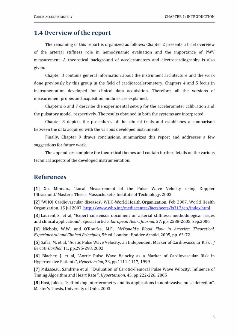
1.4 Overview of the report
The remaining of this report is organized as follows: Chapter 2 presents a brief overview
of the arterial stiffness role in hemodynamic evaluation and the importance of PWV
measurement. A theoretical background of accelerometers and electrocardiography is also
given.
Chapter 3 contains general information about the instrument architecture and the work
done previously by this group in the field of cardioaccelerometery. Chapters 4 and 5 focus in
instrumentation developed for clinical data acquisition. Therefore, all the versions of
measurement probes and acquisition modules are explained.
Chapters 6 and 7 describe the experimental set-up for the accelerometer calibration and
the pulsatory model, respectively. The results obtained in both the systems are interpreted.
Chapter 8 depicts the procedures of the clinical trials and establishes a comparison
between the data acquired with the various developed instruments.
Finally, Chapter 9 draws conclusions, summarizes this report and addresses a few
suggestions for future work.
The appendices complete the theoretical themes and contain further details on the various
technical aspects of the developed instrumentation.
References
[1] Xu, Minnan., “Local Measurement of the Pulse Wave Velocity using Doppler Ultrasound.”Master’s Thesis, Massachusetts Institute of Technology, 2002
[2] ‘WHO| Cardiovascular diseases’, WHO-World Health Organization, Feb 2007, World Health Organization. 15 Jul 2007. http://www.who.int/mediacentre/factsheets/fs317/en/index.html
[3] Laurent, S. et al, “Expert consensus document on arterial stiffness: methodological issues and clinical applications”, Special article, European Heart Journal, 27, pp. 2588-2605, Sep.2006
[4] Nichols, W.W. and O’Rourke, M.F., McDonald’s Blood Flow in Arteries: Theoretical,
Experimental and Clinical Principles, 5th ed. London: Hodder Arnold, 2005, pp. 63-72
[5] Safar, M. et al, “Aortic Pulse Wave Velocity: an Independent Marker of Cardiovascular Risk”, J Geriatr Cardiol, 11, pp.295-298, 2002
[6] Blacher, J. et al, “Aortic Pulse Wave Velocity as a Marker of Cardiovascular Risk in Hypertensive Patients”, Hypertension, 33, pp.1111-1117, 1999
[7] Milasseau, Sandrine et al, “Evaluation of Carotid-Femoral Pulse Wave Velocity: Influence of Timing Algorithm and Heart Rate ”, Hypertension, 45, pp.222-226, 2005
[8] Hast, Jukka., “Self-mixing interferometry and its applications in noninvasive pulse detection”. Master’s Thesis, University of Oulu, 2003

4
CHAPTER 2
THEORETICAL BACKGROUND
This chapter begins with an overview of the arterial stiffness role in hemodynamic
evaluation and the importance of PWV measurement. Later, section 2.3 describes in a few
words, the basic principles of accelerometers used during the development of our instrumental
prototypes. The last section, more extensive, is dedicated to electrocardiography, which was
incorporated on the acquisition modules as the main time reference.
2.1 Arterial Stiffness and Pulse Wave Velocity
2.1.1 General Concepts
I. Wave propagation in an elastic tube
An artery is a viscoelastic tube whose diameter varies with a pulsating pressure; in
addition, it will propagate pressure and flow waves, generated by the ejection of blood from the
left ventricle, at a certain velocity, which is largely determined by the elastic properties of the
arterial wall [1].
The relationship between PWV (velocity at which the pressure wave propagates along the
artery) and the elasticity of a thin-walled tube filled with an incompressible fluid is expressed by
the Moens-Korteweg Equation [2]:
√/2 (Eq.1)
From this equation, it is seen that the PWV (m/s) is related to the square root Young’s
modulus of elasticity (E), where h represents the wall thickness, r the radius and ρ the density of
fluid.
Therefore measuring the PWV leads an estimate of the stiffness of the tube. Higher
velocity corresponds to higher arterial stiffness.
It is generally agreed that many cardiovascular disorders are associated with increasing
rigidity of the arterial wall.

CARDIOACCELEROMETERY CHAPTER 2: THEORETHICAL BACKGROUND
5
II. Factors influencing arterial stiffness
A large number of publications and several reviews reported the various
pathophysiological conditions associated with increased arterial stiffness (table 2). Apart from
the dominant effect of ageing, they include physiological conditions, genetic background, CV risk
factors, CV diseases and primarily non-CV diseases [3].
Table 2 Clinical conditions associated with increased arterial stiffness. Adapted from [3].
Ageing CV risk factors CV diseases
Physiological conditions Hypertension Coronary heart disease Low birth weight Smoking Congestive heart failure Menopausa Status Obesity Fatal stroke
Lack of physical activity Hypercholesterolaemia Primarily non-CV diseases
Genetic background Impaired glucose intolerance Moderate chronic kidney disease
Parental history of hypertension
Metabolic syndrome Rheumatoid arthritis
Parental history of diabetes Type 1 diabetes Systemic vasculitis
Parental history of myocardial infarction
Type 2 diabetes Systemic lupus erythematosus
Genetic polymorphisms High C-reactive protein level
When evaluating the degree of arterial stiffness, the two major parameters to be taken in
account are age and blood pressure.
2.1.2 PWV Measurements
The measurement of PWV is generally accepted as the most simple, non-invasive, robust
and reproducible method to determine arterial stiffness [3].
Carotid-femoral PWV is a direct measurement and it is the most clinically relevant, since
the aorta and its first branches are the major components of arterial elasticity and they are
responsible for most of the pathophysiological effects of arterial stiffness.
In addition, a large amount of epidemiological studies demonstrates that aortic PWV holds
a strong predictive potential, as intermediate endpoint for CV events. In fact, it has a better
predictive value than classical CV risks entering various type of risk score [1] [3-5].
PWV is usually measured using foot-to-foot velocity method from various waveforms.
These are usually obtained at the right common carotid artery and right femoral artery, and the
time delay (∆t or transit time) measured between the feet of the two waveforms (figure 1). A
variety of different waveforms can be used including pressure, distension, and Doppler. For
further reading: [2, 3].
CARDIOACCELEROMETERY CHAPTER 2: THEORETHICAL BACKGROUND
6
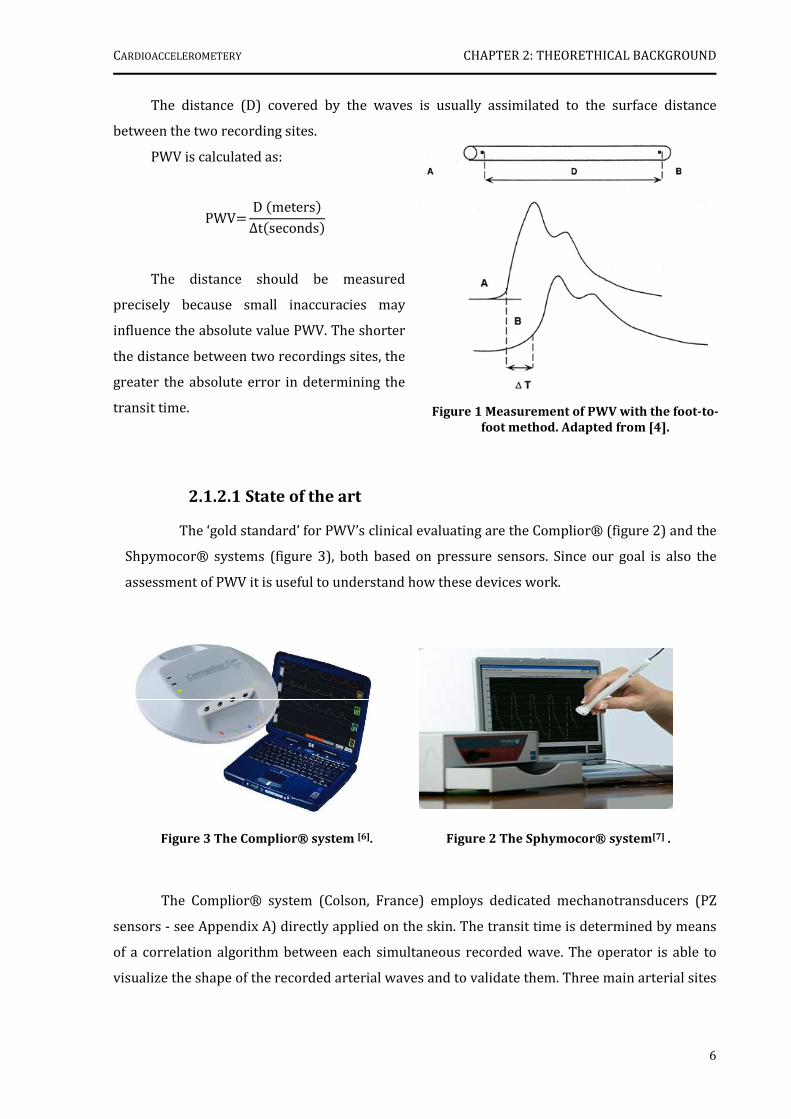
The distance (D) covered by the waves is usually assimilated to the surface distance
between the two recording sites.
PWV is calculated as:
PWV D meters ∆tseconds
The distance should be measured
precisely because small inaccuracies may
influence the absolute value PWV. The shorter
the distance between two recordings sites, the
greater the absolute error in determining the
transit time.
2.1.2.1 State of the art
The ‘gold standard’ for PWV’s clinical evaluating are the Complior® (figure 2) and the
Shpymocor® systems (figure 3), both based on pressure sensors. Since our goal is also the
assessment of PWV it is useful to understand how these devices work.
The Complior® system (Colson, France) employs dedicated mechanotransducers (PZ
sensors - see Appendix A) directly applied on the skin. The transit time is determined by means
of a correlation algorithm between each simultaneous recorded wave. The operator is able to
visualize the shape of the recorded arterial waves and to validate them. Three main arterial sites
Figure 3 The Complior® system [6]. Figure 2 The Sphymocor® system[7] .
Figure 1 Measurement of PWV with the foot-to-
foot method. Adapted from [4].

CARDIOACCELEROMETERY CHAPTER 2: THEORETHICAL BACKGROUND
7
can be evaluated, mainly the aortic trunk (carotid-femoral) and the upper (carotid-brachial ) and
lower (femoral-dorsalis pedis) limbs [3] [6] .
In the Shpymocor® system (ArtCor, Australia), a single high-fidelity applanation
tonometer (Millar®) to obtain a proximal (i.e. carotid artery) and distal pulse (i.e. radial or
femoral arteries) recorded sequentially a short time apart and calculates PWV from the transit
time between the two arterial sites, determined in relation to the R-wave of the
electrocardiogram1 (ECG). The time between ECG and proximal pulse is subtracted from the
time between ECG and distal pulse to obtain the pulse transit time. The initial part of the
pressure waveform is use as a reference point. It is also possible to check offline the variability
of measurement over a range of pulses, according to each algorithm [3] [7].
1 See section 2.3.2.
CARDIOACCELEROMETERY CHAPTER 2: THEORETHICAL BACKGROUND
8
2.2 Accelerometric Sensors
2.2.1 Introduction
Acceleration2 is an important parameter for general-purpose absolute motion, orientation,
tilt, vibration and shock sensing measurements and can be assessed by accelerometers [8].
Accelerometers are commercially available in a wide variety of ranges and types to meet
diverse application requirements. Their low-cost, small size (MEMS3 devices), light weight and
robustness, makes them a fundamental and increasingly common device in many technological
areas.
In general, accelerometers are preferred over displacement and velocity sensors for the
following reasons [9]:
1. They deliver 1, 2 or 3 measurement-axes and have a wide frequency range from DC
to very high values, in such a way that steady accelerations can easily be measured;
2. Measurement of transients and shocks can be made more easily than with
displacement or velocity sensing;
3. Displacement and velocity can be obtained by simple integration of acceleration
(integration is preferred over differentiation).
In this section, common concepts underlying accelerometers usage (operation and
calibration principles, main types and applications) will be briefly introduced.
2.2.2 General Concepts
Theory of operation
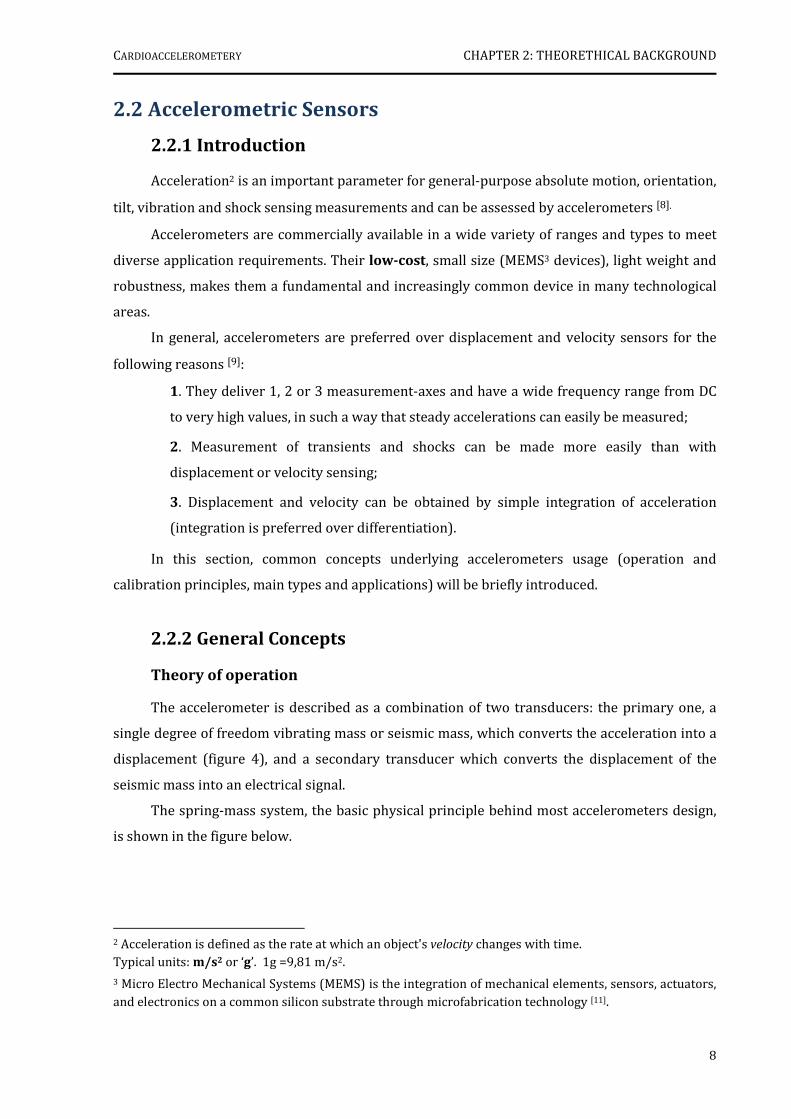
The accelerometer is described as a combination of two transducers: the primary one, a
single degree of freedom vibrating mass or seismic mass, which converts the acceleration into a
displacement (figure 4), and a secondary transducer which converts the displacement of the
seismic mass into an electrical signal.
The spring-mass system, the basic physical principle behind most accelerometers design,
is shown in the figure below.
2 Acceleration is defined as the rate at which an object's velocity changes with time. Typical units: m/s2 or ‘g’. 1g =9,81 m/s2.
3 Micro Electro Mechanical Systems (MEMS) is the integration of mechanical elements, sensors, actuators,
and electronics on a common silicon substrate through microfabrication technology [11].
CARDIOACCELEROMETERY CHAPTER 2: THEORETHICAL BACKGROUND
9
Figure 4 The basic spring mass system accelerometer [8].
A mass m that is free to slide on a base is connected to it by a spring. This spring that is in
its unextended state exerts no force on the mass.
If this system undergoes a acceleration, then, by Newton's law, a resultant force equal to
ma will be exerted on the mass. This force causes the mass to either compress or expand the
spring under the constraint that F=ma=kx. Hence an acceleration a will cause the mass to be
displaced by / or, conversely, if a displacement of x is observed, it is know that the mass
has undergone an acceleration of /.
Note that this model system only responds to accelerations along the length of the spring.
This is referred to as a single axis accelerometer. In order to measure multiple axes of
acceleration, this system needs to be replicated along each of the required axes.
Main types and applications
According to the type of secondary transducer accelerometers are generally classified as
piezoelectric, potentiometric, reluctive, servo, strain gauge, capacitive or vibrating element. For
further reading: [10].
Amongst its main application areas the following are worth mentioning:
1. Automotive (airbag sensors, active suspensions, roll over sensing, GPS, vibration
monitoring, safety related testing)
2. Aeronautic and defence (ammunition & missile guidance, aeronautic instruments)
3. Medical (pacemaker, human motion analysis, wheel chair stabilization)
4. Industrial
Calibration
Calibration refers to the process of determining the relation between the output (or
response) of a measuring sensor/instrument and the value of the input quantity, a measurement
standard [9].

CARDIOACCELEROMETERY CHAPTER 2: THEORETHICAL BACKGROUND
10
If the sensor has a linear response then its sensitivity4 is determined by the slope of the
calibration curve.
An accelerometer can be calibrated by static or dynamic methods. To perform a static
calibration of the accelerometer, the device is subjected to one or several levels of constant
acceleration. The simplest method, for low g applications is to use the force of gravity, since it is
the most stable, accurate and convenient acceleration reference available (figure 5) [12].
The dynamic calibration is usually obtained using an electrodynamic shaker. This device is
designed to oscillate in a sinusoidal motion with variable frequencies and amplitudes.
The relationship between this variables, which are accurately measured, and the
accelerometer’s output is then determined.
(a) (b)
4 The sensor’s sensitivity measures the level of variation of the output regarding variations applied to its
input. For example, an accelerometer is very sensible if small variations on the acceleration cause large
variations in its output [9].
Figure 5 Flip Calibration [12]: (a) +1g (b) -1g.
To calibrate, the accelerometer’s measurement axis is pointed directly at the earth. The 1 g reading is saved and the sensor is rotated 180° to measure –1 g. Using the two
readings, the sensitivity is: Sensitivity = [A – B]/2 g
A = Accelerometer output with axis oriented to +1 g;
B = Accelerometer output with axis oriented to –1 g;
CARDIOACCELEROMETERY CHAPTER 2: THEORETHICAL BACKGROUND
11
2.3 Electrocardiography
2.3.1 Introduction
One of the main techniques for diagnosing heart‘s electrical and mechanical condition is
based on the electrocardiogram [13].
An electrocardiogram is a recording of the electrical activity on the body surface generated
by the heart.
ECG measurement information is collected by skin electrodes placed at designated
locations on the body. By convention, the electrodes are placed on each arm and leg, and six
electrodes are placed at defined locations on the chest. The particular arrangement of two
electrodes (one positive and one negative) with respect to a third one (the ground) is called a
lead [14] [15].
There are three types of ECG leads: bipolar limb leads, augmented unipolar limb leads and
unipolar precordial leads (table 3) [16].
In a standard clinical ECG, all leads are recorded simultaneously, giving rise to what is
called a 12-lead ECG. In monitoring applications, typically one or two leads are used, since the
principal goal of these is to reliably recognize each heartbeat and perform rhythm analysis [13].
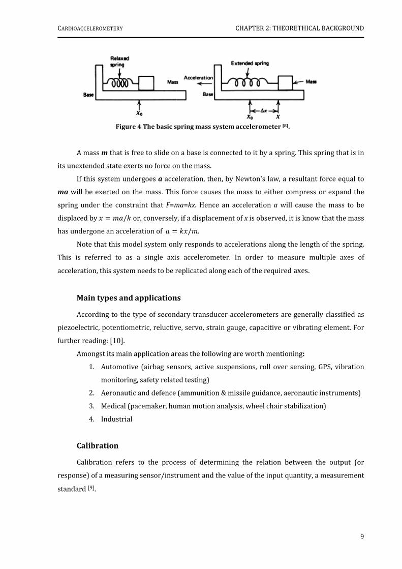
Table 3 Types of ECG leads. The bipolar leads utilize a single positive and a single negative electrode between which electrical potentials are measured. The unipolar leads have a single positive recording electrode and utilize a combination of the other electrodes to serve as a composite negative electrode.
Each of the 12 leads provides spatial information about heart’s electrical activity in three approximately orthogonal directions: right ↔ left; superior ↔ inferior; anterior ↔ posterior [5] [6]. Lead place diagrams
can be seen in Appendix A.
Leads Types Electrodes Location
Electrical activity
recorded: Spatial
Information
Bipolar Limb
I RA (-) to LA (+)1
Frontal Plane
Right Left, or lateral
II RA (-) to LF (+) Superior Inferior
III LA (-) to LF (+) Superior Inferior
Unipolar
Augmented aVR RA (+) to [LA & LF] (-) Rightward aVL LA (+) to [RA & LF] (-) Leftward aVF LF (+) to [RA & LA] (-) Inferior
Precordial V1, V2, V3
Chest Horizontal
Plane
Posterior Anterior
V4, V5, V6 Right Left, or lateral
1 RA: right arm; LA: left arm; LF: left foot (-) negative electrode, (+) positive electrode
CARDIOACCELEROMETERY CHAPTER 2: THEORETHICAL BACKGROUND
12
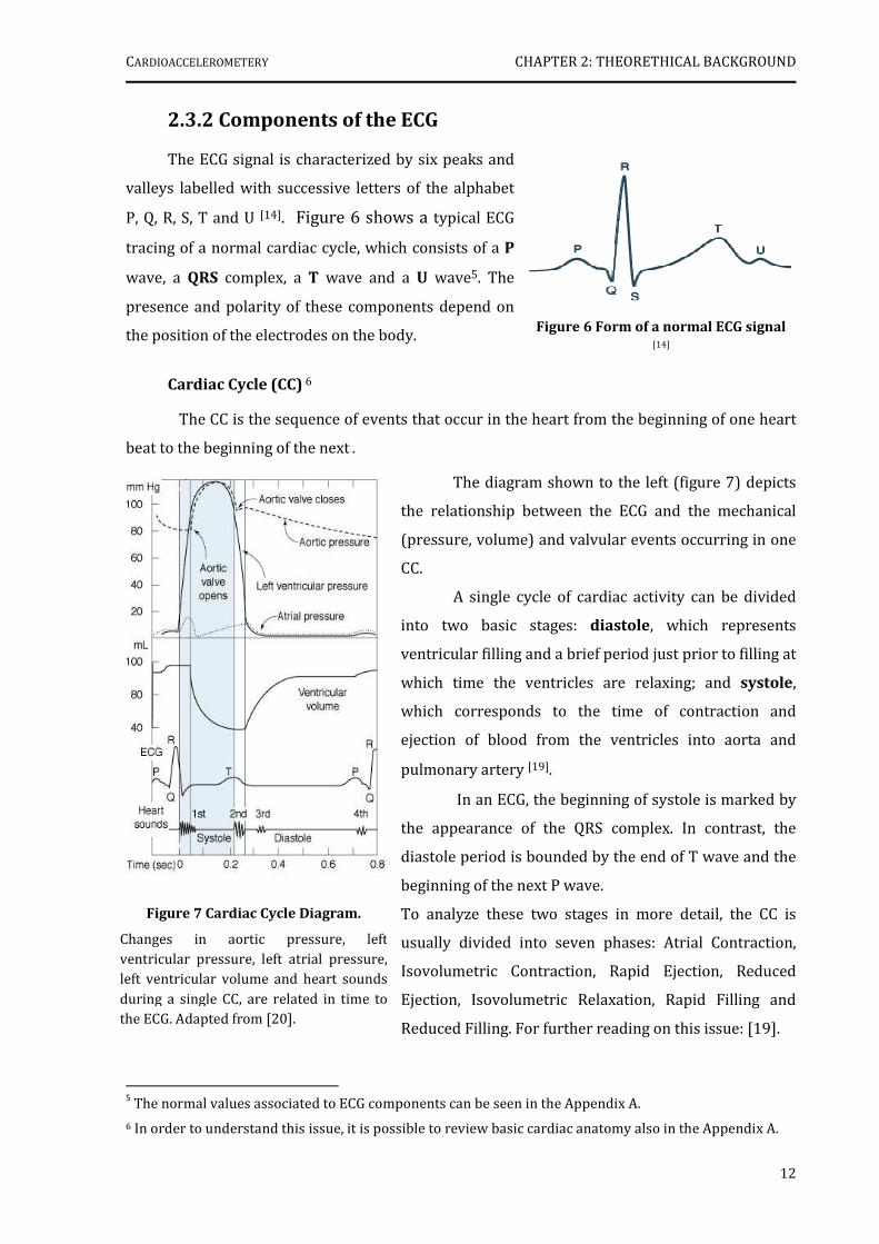
Figure 7 Cardiac Cycle Diagram.
Changes in aortic pressure, left ventricular pressure, left atrial pressure, left ventricular volume and heart sounds
during a single CC, are related in time to the ECG. Adapted from [20].
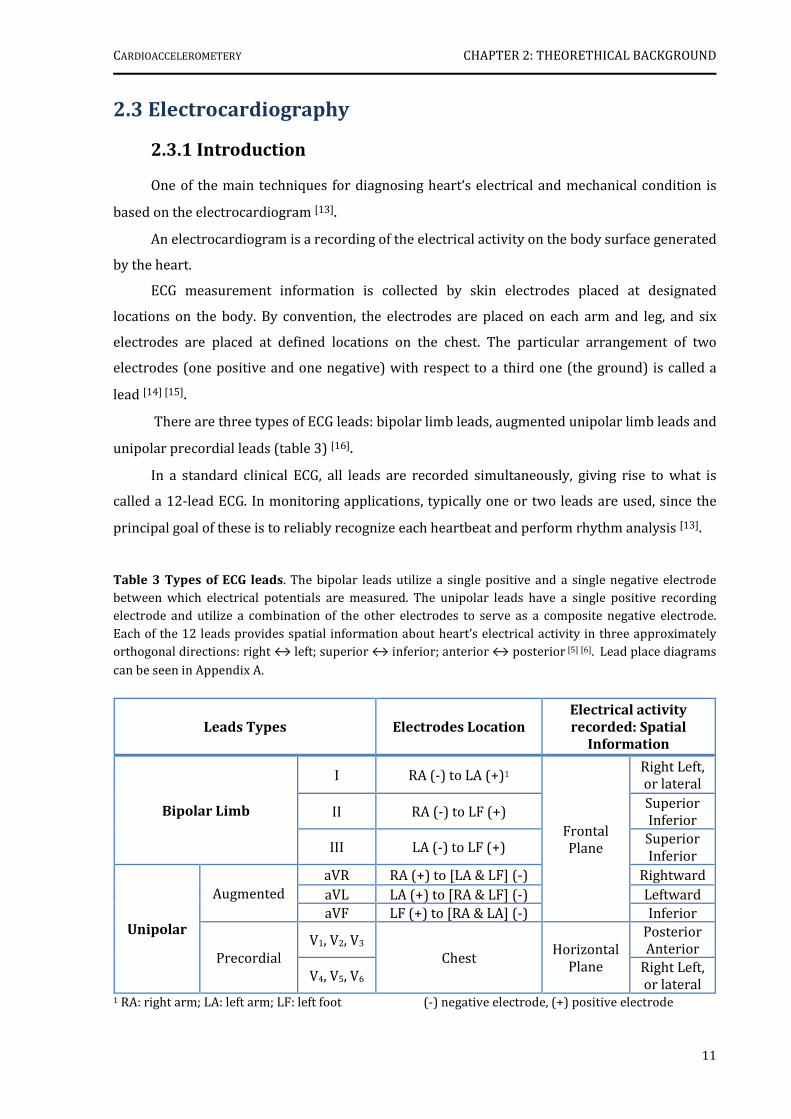
2.3.2 Components of the ECG
The ECG signal is characterized by six peaks and
valleys labelled with successive letters of the alphabet
P, Q, R, S, T and U [14]. Figure 6 shows a typical ECG
tracing of a normal cardiac cycle, which consists of a P
wave, a QRS complex, a T wave and a U wave5. The
presence and polarity of these components depend on
the position of the electrodes on the body.
Cardiac Cycle (CC) 6
The CC is the sequence of events that occur in the heart from the beginning of one heart
beat to the beginning of the next .
The diagram shown to the left (figure 7) depicts
the relationship between the ECG and the mechanical
(pressure, volume) and valvular events occurring in one
CC.
A single cycle of cardiac activity can be divided
into two basic stages: diastole, which represents
ventricular filling and a brief period just prior to filling at
which time the ventricles are relaxing; and systole,
which corresponds to the time of contraction and
ejection of blood from the ventricles into aorta and
pulmonary artery [19].
In an ECG, the beginning of systole is marked by
the appearance of the QRS complex. In contrast, the
diastole period is bounded by the end of T wave and the
beginning of the next P wave.
To analyze these two stages in more detail, the CC is
usually divided into seven phases: Atrial Contraction,
Isovolumetric Contraction, Rapid Ejection, Reduced
Ejection, Isovolumetric Relaxation, Rapid Filling and
Reduced Filling. For further reading on this issue: [19].
5 The normal values associated to ECG components can be seen in the Appendix A.
6 In order to understand this issue, it is possible to review basic cardiac anatomy also in the Appendix A.
Figure 6 Form of a normal ECG signal
[14]
CARDIOACCELEROMETERY CHAPTER 2: THEORETHICAL BACKGROUND
13
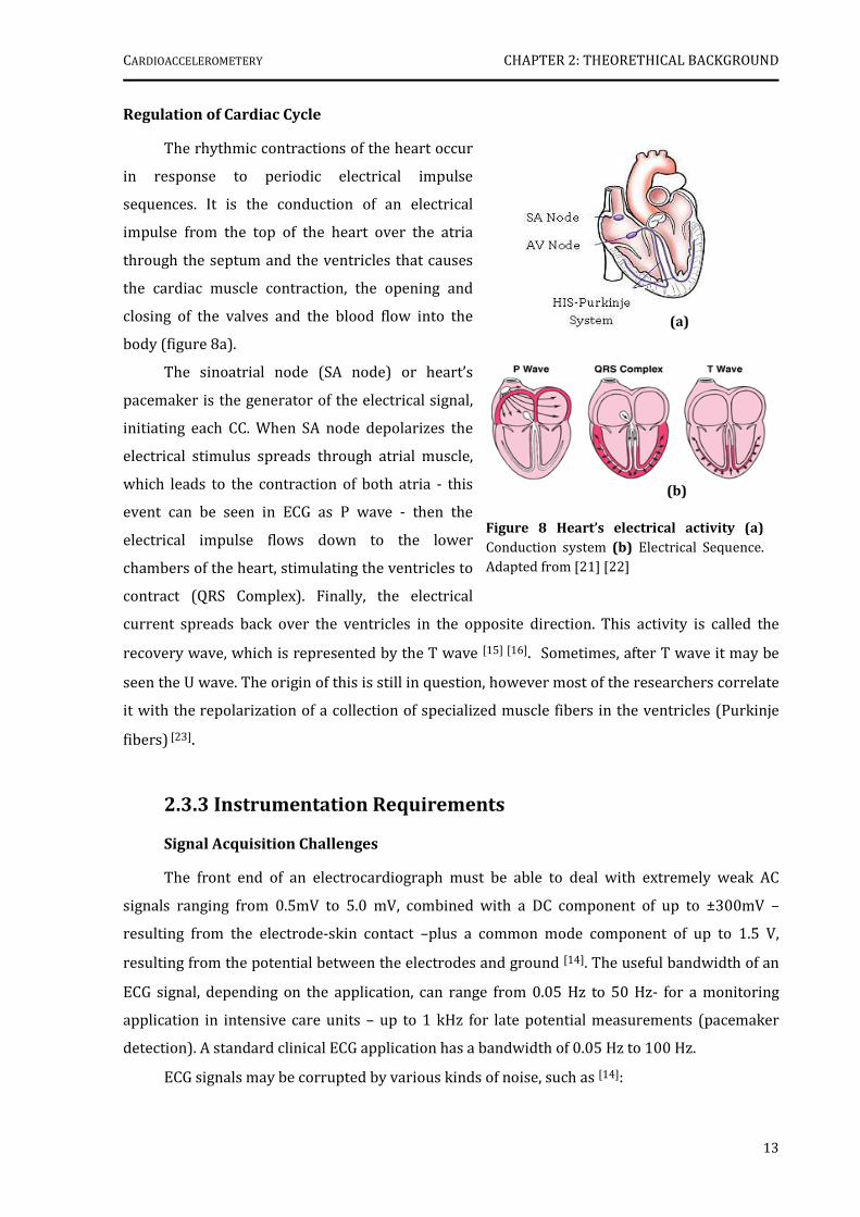
Figure 8 Heart’s electrical activity (a)
Conduction system (b) Electrical Sequence. Adapted from [21] [22]
Regulation of Cardiac Cycle
The rhythmic contractions of the heart occur
in response to periodic electrical impulse
sequences. It is the conduction of an electrical
impulse from the top of the heart over the atria
through the septum and the ventricles that causes
the cardiac muscle contraction, the opening and
closing of the valves and the blood flow into the
body (figure 8a).
The sinoatrial node (SA node) or heart’s
pacemaker is the generator of the electrical signal,
initiating each CC. When SA node depolarizes the
electrical stimulus spreads through atrial muscle,
which leads to the contraction of both atria - this
event can be seen in ECG as P wave - then the
electrical impulse flows down to the lower
chambers of the heart, stimulating the ventricles to
contract (QRS Complex). Finally, the electrical
current spreads back over the ventricles in the opposite direction. This activity is called the
recovery wave, which is represented by the T wave [15] [16]. Sometimes, after T wave it may be
seen the U wave. The origin of this is still in question, however most of the researchers correlate
it with the repolarization of a collection of specialized muscle fibers in the ventricles (Purkinje
fibers) [23].
2.3.3 Instrumentation Requirements
Signal Acquisition Challenges
The front end of an electrocardiograph must be able to deal with extremely weak AC
signals ranging from 0.5mV to 5.0 mV, combined with a DC component of up to ±300mV –
resulting from the electrode-skin contact –plus a common mode component of up to 1.5 V,
resulting from the potential between the electrodes and ground [14]. The useful bandwidth of an
ECG signal, depending on the application, can range from 0.05 Hz to 50 Hz- for a monitoring
application in intensive care units – up to 1 kHz for late potential measurements (pacemaker
detection). A standard clinical ECG application has a bandwidth of 0.05 Hz to 100 Hz.
ECG signals may be corrupted by various kinds of noise, such as [14]:
(b)
(a)
CARDIOACCELEROMETERY CHAPTER 2: THEORETHICAL BACKGROUND
14
• Power-line interference: 50–60 Hz pickup and harmonics from the power mains;
• Electrode contact noise: variable contact between the electrode and the skin, causing
baseline drift;
• Motion artefacts: shifts in the baseline caused by changes in the electrode-skin
impedance;
• Muscle contraction: electromyogram-type signals are generated and mixed with the ECG
signals;
• Respiration, causing drift in the baseline;
• Electromagnetic interference from other electronic devices, with the electrode wires
serving as antennas;
• Noise coupled from other electronic devices, usually at high frequencies;
For meaningful and accurate detection, it is necessary to filter out all these noises sources.
Typical Measurement System
Figure 9 shows a block diagram of a typical single-channel electrocardiograph. The ECG
system comprises five basic stages. In the first one the bioelectrodes convert the ionic current
flow of the body to an electron flow of the metallic wire. The efficient acquisition by these
electrodes relies on a gel with a high ionic concentration. This acts as the transducer at the
tissue-electrode interface [16].
Then an instrumentation amplifier (IA), with a high gain and common mode rejection
ratio (CMRR), attenuates the signals that are common to both inputs and amplifies the difference
between the two signals. Due to this some of the noise is eliminated. To further reject 50Hz and
60 Hz noise, an operational amplifier (op amp) deriving common-mode voltage is used to invert
the common-mode signal and drive it back into the patient trough the right leg [14][24].
Subsequently, it is visible the presence of an opto isolator7, which allows galvanic
isolation; some analog filters (high pass filter, low pass filter and notch); an ADC8 and a DSP9,
which permit the conversion to digital domain and the communication to computer,
respectively[14] .
7 This technology can be substituted by other with the same function, e.g.: magnetic induction.
8 Analogic Digital Converter.
9 Microprocessor or Microcontroller.

CARDIOACCELEROMETERY CHAPTER 2: THEORETHICAL BACKGROUND
15
References
[1] Nichols, W.W. and O’Rourke, M.F., McDonald’s Blood Flow in Arteries: Theoretical,
Experimental and Clinical Principles, 5th ed. London: Hodder Arnold, 2005, pp. 54-72
[2] Xu, Minnan., “Local Measurement of the Pulse Wave Velocity using Doppler Ultrasound.”Master’s Thesis, Massachusetts Institute of Technology, 2002
[3] Laurent, S. et al, “Expert consensus document on arterial stiffness: methodological issues and clinical applications”, Special article, European Heart Journal, 27, pp. 2588-2605, Sep.2006
[4] Safar, M. et al, “Aortic Pulse Wave Velocity: an Independent Marker of Cardiovascular Risk”, J Geriatr Cardiol, 11, pp.295-298, 2002
[5] Blacher, J. et al, “Aortic Pulse Wave Velocity as a Marker of Cardiovascular Risk in Hypertensive Patients”, Hypertension, 33, pp.1111-1117, 1999
[6] Figure at: http://www.pmsinstruments.co.uk/Complior%20SP.htm
[7] Figure at: http://atcormedical.com/sphygmocor.html
[8] Pereira, Helena, “Acelerómetros”. Monography, Sensores e Sinais Biomédicos discipline Universidade de Coimbra, January 2006
[9] Webster, John G., Measurement, Instrumentation and Sensors Handbook CRCnetBASE. 1st ed. New York: CRC Press LLC, 1999, pp: 454-481
[10] Muramatsu, Brandon. "Accelerometer." 16 Jan 2000. University of Berkeley. 7 Sep 2007 http://bits.me.berkeley.edu/beam/acc_1.html
[11] "What is MEMS Technology?." MEMS and Nanotechnology Clearinghouse. MEMS and Nanotechnology Clearinghouse. 7 Sep 2007 http://www.memsnet.org/mems/what-is.html
[12] Stilson , Tim. "Accelerometer." Input/Data Acquisition System Design for Human Computer Interfacing. 17 Oct 1996. 7 Sep 2007 http://soundlab.cs.princeton.edu/learning/tutorials/sensors/node9.html
[13] Tompkins, J. Willis, Biomedical Digital Signal Processing, Prentice-Hall, Inc., 1993, pp.24-39
[14] Bosch, E., “ECG Front-End Design is Simplified with MicroConverter”, Analog Dialogue 37-11, November 2003, www.analog.com/analogdialogue
Figure 9 Typical single-channel electrocardiograph. Adapted from [14].

CARDIOACCELEROMETERY CHAPTER 2: THEORETHICAL BACKGROUND
16
[15] Biopac Systems, Inc., “Lesson 5 Electrocardiography I”, Physiology Lessons for use with the Biopac Student Lab, www.biopac.com
[16] Berbari, E.J., “Principles of Electrocardiography”, The Biomedical Engineering Handbook,
2nd ed. Boca Raton: CRC Press LLC, 2000, Chapter 13
[17] Yanowitz, Frank. "Lesson 1: The Standard 12 Lead ECG." ECG learning center. 5 Jun 2006. 2 Sep 2007 http://library.med.utah.edu/kw/ecg/ecg_outline/Lesson1/index.html
[18] Klabunde, Richard . "ECG leads." Cardiovascular Physiology Concepts. 01 Jan 2007. 2 Sep 2007 http://cvphysiology.com/Arrhythmias/A013.htm
[19] Klabunde, Richard . "ECG leads." Cardiovascular Physiology Concepts. 13 Apr 2007. 2 Sep 2007 http://cvphysiology.com/Heart%20Disease/HD002.htm
[20]Figure at: http://connection.lww.com/Products/porth7e/documents/Ch23/jpg/23_015.jpg
[21] Figure at: http://www.heartcare4u.com/hearts/normalheart.jpg
[22] Figure at: www.merck.com/mmhe/sec03/ch021/ch021c.html
[23] Yanowitz, Frank. "Lesson 12: Nice Seeing U wave." ECG learning center. 5 Jun 2006. 2 Sep 2007 < http://library.med.utah.edu/kw/ecg/ecg_outline/Lesson12/index.html>
[24] TI medical applications
[25] Figure at: http://www.bg.ic.ac.uk/Staff/khparker/homepage/BSc_lectures/2002/Heart_anatomy.jpg
[26]Figure at: http://www.doc.ic.ac.uk/~giso/projects/arrhythmia/node4.html
[27] Figure at: www.publicsafety.net/12lead_dx.htm
[28]Figure at: www.cvphysiology.com/Arrhythmias/A013c.htm
[29]Figure at: http://butler.cc.tut.fi/~malmivuo/bem/bembook/15/15.htm
17
CHAPTER 3
PROCESS METHODOLOGY
This chapter presents the work developed by the hemodynamic team, previously to the
Project starting date, in the field of cardioaccelerometery.
3.1 Introduction
The development of an accelerometer based instrument started some months before the
beginning of the Project discipline. At that time, its application was related with the maintenance
and monitoring of railways equipments.
However, lab experiments were carried out using the same instrument in the carotid
artery of human subjects, showing promising results.
The potential of these results was then discussed with a cardiologist and a new objective
arose: the assessment of PWV with accelerometers. In order to achieve this idea a first
accelerometer based instrument was designed and trimmed to clinical experiments.
3.2 Measurement System Architecture
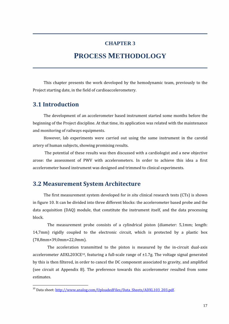
The first measurement system developed for in situ clinical research tests (CTs) is shown
in figure 10. It can be divided into three different blocks: the accelerometer based probe and the
data acquisition (DAQ) module, that constitute the instrument itself, and the data processing
block.
The measurement probe consists of a cylindrical piston (diameter: 5,1mm; length:
14,7mm) rigidly coupled to the electronic circuit, which is protected by a plastic box
(78,8mm×39,0mm×22,0mm).
The acceleration transmitted to the piston is measured by the in-circuit dual-axis
accelerometer ADXL203CE10, featuring a full-scale range of ±1.7g. The voltage signal generated
by this is then filtered, in order to cancel the DC component associated to gravity, and amplified
(see circuit at Appendix B). The preference towards this accelerometer resulted from some
estimates.
10
Data sheet: http://www.analog.com/UploadedFiles/Data_Sheets/ADXL103_203.pdf.

CARDIOACCELEROMETERY CHAPTER 3: PROCESS METHODOLOGY
18
USB
Restart
Power Supply
Measurement probe
Data Acquisition
Module
IInnssttrruummeenntt AArrcchhiitteeccttuurree
Data Processing
Matlab®
NI USB 6008©
NI-DAQmx© Software
Figure 11 NI USB-6008© [1].
Table 4 Some NI USB-6008 Specifications [1].
Specifications Summary
USB Bus Type
8 analog inputs (resolution: 12-bit; sampling rate: 10Ks/s);
2 analog outputs (resolution: 12-bits; update rate: 150Ks/s);
12 digital input/output;
32-bit counter;
NI-DAQmx© driver software and
NI LabVIEW SignalExpress LE interactive data-logging software;
Figure 10 General measurement system architecture.
The DAQ module used in this measurement system is the NI USB-6008©11, shown in figure
11. This device is based in an 8051 microcontroller, can sample up to 10Ks/s and comes with a
driver software for interactive configuration and data acquisition running on Windows
Operative System: the NI-DAQmx© (table 4). This software includes VI Logger Lite, a
configuration software package, which is used in this architecture for data logging.
After the data logging, it follows up the data processing, where the files are saved in a .txt
format and processed in Matlab®.
11
Data sheet at: http://www.ni.com/pdf/products/us/20043762301101dlr.pdf.
CARDIOACCELEROMETERY CHAPTER 3: PROCESS METHODOLOGY
19
3.3 Clinical Trials
3.3.1 Data Acquisition
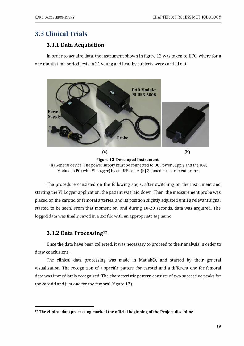
In order to acquire data, the instrument shown in figure 12 was taken to IIFC, where for a
one month time period tests in 21 young and healthy subjects were carried out.
The procedure consisted on the following steps: after switching on the instrument and
starting the VI Logger application, the patient was laid down. Then, the measurement probe was
placed on the carotid or femoral arteries, and its position slightly adjusted until a relevant signal
started to be seen. From that moment on, and during 10-20 seconds, data was acquired. The
logged data was finally saved in a .txt file with an appropriate tag name.
3.3.2 Data Processing12
Once the data have been collected, it was necessary to proceed to their analysis in order to
draw conclusions.
The clinical data processing was made in Matlab®, and started by their general
visualization. The recognition of a specific pattern for carotid and a different one for femoral
data was immediately recognized. The characteristic pattern consists of two successive peaks for
the carotid and just one for the femoral (figure 13).
12 The clinical data processing marked the official beginning of the Project discipline.
Figure 12 Developed Instrument.
(a) General device: The power supply must be connected to DC Power Supply and the DAQ
Module to PC (with VI Logger) by an USB cable. (b) Zoomed measurement probe. (a
Power
Supply
DAQ Module:
NI USB-6008
Probe
(a) (b)

CARDIOACCELEROMETERY CHAPTER 3: PROCESS METHODOLOGY
20
1 2 3 4 5 6 7 8 9 10-0.8
-0.6
-0.4
-0.2
0
0.2
0.4
s
V
1 2 3 4 5 6 7 8 9 10
-1
-0.5
0
0.5
1
1.5
s
VIn order to extract more information about patterns repeatability, an algorithm was
developed, whose main purpose was to relate the peaks of each acquisition.
This algorithm consisted in the following main steps:
Step 1: File loading and visualization;
Step 2: Filtering (application of a band-pass filter);
Step 3: Selection of peaks;
Step 4: Peaks Adjustment;
Step 6: Overlapping of the selected peaks;
Step 7: Mean determination of overlapped peaks;
Step 8: Data saving.
Figure 14 shows the result from the application of steps 6 and 7 to either a carotid or
femoral files of two patients.
(a) (b)
Figure 13 Original Signals of a young and healthy subject, obtained with the accelerometer based
instrument and visualized in Matlab®: (a) Carotid signal. (b) Femoral Signal.
P2
(a) (b)
P1
CARDIOACCELEROMETERY CHAPTER 3: PROCESS METHODOLOGY
21
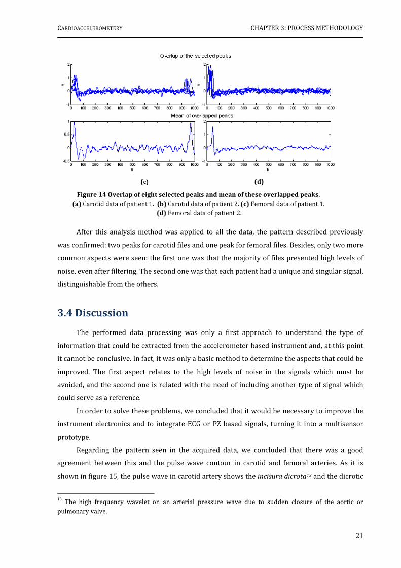
After this analysis method was applied to all the data, the pattern described previously
was confirmed: two peaks for carotid files and one peak for femoral files. Besides, only two more
common aspects were seen: the first one was that the majority of files presented high levels of
noise, even after filtering. The second one was that each patient had a unique and singular signal,
distinguishable from the others.
3.4 Discussion
The performed data processing was only a first approach to understand the type of
information that could be extracted from the accelerometer based instrument and, at this point
it cannot be conclusive. In fact, it was only a basic method to determine the aspects that could be
improved. The first aspect relates to the high levels of noise in the signals which must be
avoided, and the second one is related with the need of including another type of signal which
could serve as a reference.
In order to solve these problems, we concluded that it would be necessary to improve the
instrument electronics and to integrate ECG or PZ based signals, turning it into a multisensor
prototype.
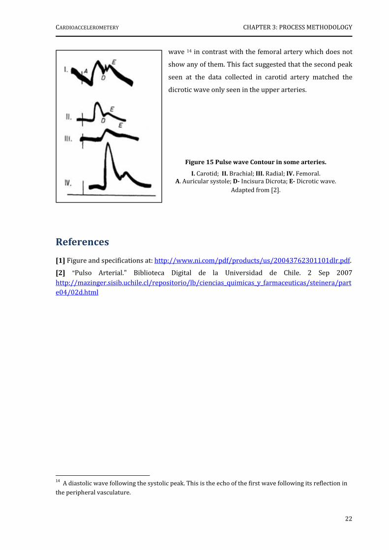
Regarding the pattern seen in the acquired data, we concluded that there was a good
agreement between this and the pulse wave contour in carotid and femoral arteries. As it is
shown in figure 15, the pulse wave in carotid artery shows the incisura dicrota13 and the dicrotic
13
The high frequency wavelet on an arterial pressure wave due to sudden closure of the aortic or
pulmonary valve.
(c) (d)
Figure 14 Overlap of eight selected peaks and mean of these overlapped peaks.
(a) Carotid data of patient 1. (b) Carotid data of patient 2. (c) Femoral data of patient 1.
(d) Femoral data of patient 2.
CARDIOACCELEROMETERY CHAPTER 3: PROCESS METHODOLOGY
22
wave 14 in contrast with the femoral artery which does not
show any of them. This fact suggested that the second peak
seen at the data collected in carotid artery matched the
dicrotic wave only seen in the upper arteries.
References
[1] Figure and specifications at: http://www.ni.com/pdf/products/us/20043762301101dlr.pdf.
[2] "Pulso Arterial." Biblioteca Digital de la Universidad de Chile. 2 Sep 2007
http://mazinger.sisib.uchile.cl/repositorio/lb/ciencias_quimicas_y_farmaceuticas/steinera/parte04/02d.html
14
A diastolic wave following the systolic peak. This is the echo of the first wave following its reflection in
the peripheral vasculature.
Figure 15 Pulse wave Contour in some arteries.
I. Carotid; II. Brachial; III. Radial; IV. Femoral. A. Auricular systole; D- Incisura Dicrota; E- Dicrotic wave.
Adapted from [2].

23
CHAPTER 4
MEASUREMENT PROBES
The design of the measurement probe is crucial to the success of an efficient
accelerometric instrument. This is the reason why this chapter is entirely devoted to the
description of the several versions developed throughout this project.
Note – Some concepts depicted in this chapter may be protected by international patents.
4.1 Introduction
The analysis of the first data bunch (section 3.3.2) immediately showed a number of
drawbacks and, consequently, the need to improve the instrument in many ways.
Concerning the measurement probe, the first perception was that the mechanical coupling
between the pulsating tissues and the sensor was not efficient which greatly impaired the signal
to noise ratio at the output.
It was very clearly the need to modify the rigid coupling between the piston and the
electronic circuit, identified as a major noise source. In fact, the second version of the
measurement probe arose from this adjustment and it featured a spring loaded coupling
between the piston and the sensor. It was therefore designated as spring-loaded probe (SLP).
Clinical experiments carried out with the SLP (chapter 8), however, showed that the final
noise level, mainly the one that was attributed to the operator itself, was still very high. A new
design was sorted out to remove this problem and another was built, based on a mechanically
differential scheme that used two aligned accelerometer sensors. For obvious reasons, we have
named this probe differential probe (DP).
The fourth and last probe version was developed in the final stage of this work and joined
the concepts of all the other versions adding the ability of integrating a PZ transducer into the
piston. This probe, which we called hybrid, was used only for data acquisition in the pulsatory
model, described in chapter 7.
CARDIOACCELEROMETERY CHAPTER 4: MEASUREMENT PROBES
24
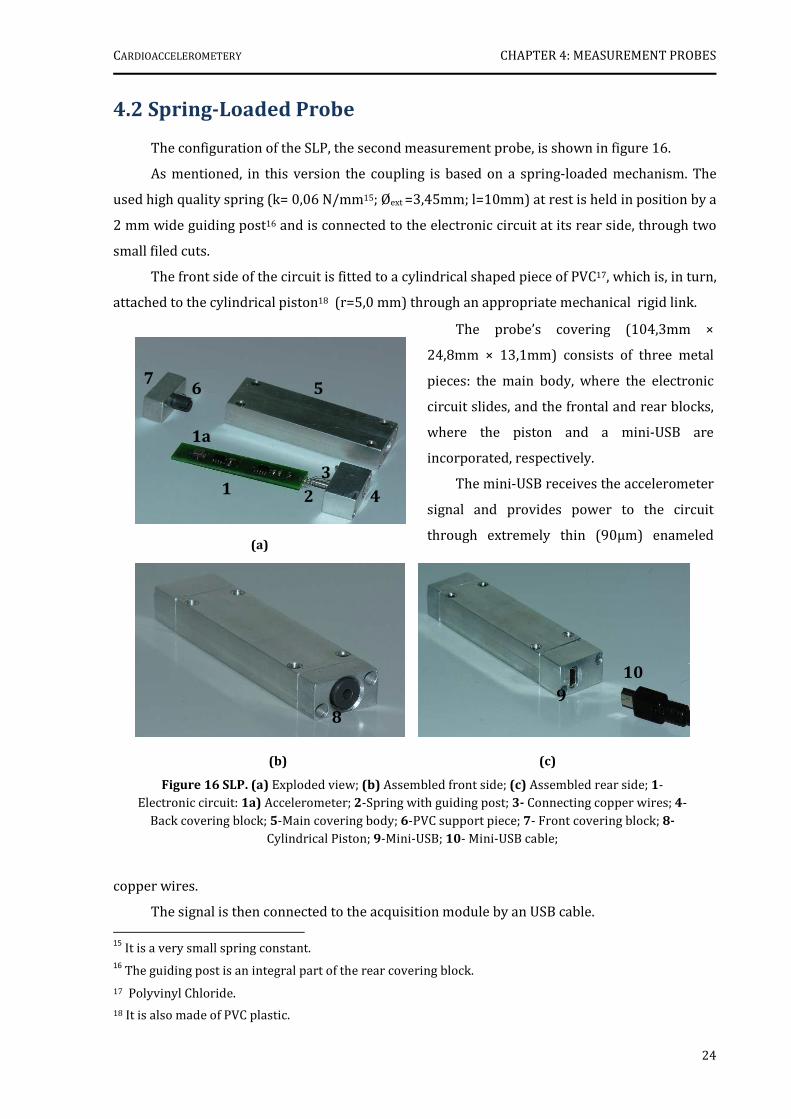
(b) (c)
Figure 16 SLP. (a) Exploded view; (b) Assembled front side; (c) Assembled rear side; 1- Electronic circuit: 1a) Accelerometer; 2-Spring with guiding post; 3- Connecting copper wires; 4-
Back covering block; 5-Main covering body; 6-PVC support piece; 7- Front covering block; 8-
Cylindrical Piston; 9-Mini-USB; 10- Mini-USB cable;
4.2 Spring-Loaded Probe
The configuration of the SLP, the second measurement probe, is shown in figure 16.
As mentioned, in this version the coupling is based on a spring-loaded mechanism. The
used high quality spring (k= 0,06 N/mm15; Øext =3,45mm; l=10mm) at rest is held in position by a
2 mm wide guiding post16 and is connected to the electronic circuit at its rear side, through two
small filed cuts.
The front side of the circuit is fitted to a cylindrical shaped piece of PVC17, which is, in turn,
attached to the cylindrical piston18 (r=5,0 mm) through an appropriate mechanical rigid link.
copper wires.
The signal is then connected to the acquisition module by an USB cable. 15
It is a very small spring constant. 16
The guiding post is an integral part of the rear covering block.
17 Polyvinyl Chloride.
18 It is also made of PVC plastic.
The probe’s covering (104,3mm ×
24,8mm × 13,1mm) consists of three metal
pieces: the main body, where the electronic
circuit slides, and the frontal and rear blocks,
where the piston and a mini-USB are
incorporated, respectively.
The mini-USB receives the accelerometer
signal and provides power to the circuit
through extremely thin (90µm) enameled
copp (a)
8
9
10
3
5
1
1a
2 4
5 7
3
6

CARDIOACCELEROMETERY CHAPTER 4: MEASUREMENT PROBES
25
Figure 17 Schematic of the forces applied on the
SLP during data acquisition.
The presented electronic circuit also contains the ADXL203CE accelerometer with
capacitive coupling and a gain stage (≈20). The circuit schematic can be seen at Appendix B.
Model of the Spring-Loaded Mechanism
A close examination of the SLP’s mode of operation shows that it is possible to establish a
relationship between the force exerted on the piston (F), the spring displacement (x), the
probe’s movable mass (m), and the acceleration of the movable mass (a), through the Newton’s
second law: ! " #$ %&
where, k = spring constant in N/m
[F ] = N;
[x]= m;
[m]= Kg;
[a]= m/s2
The forces which act on the
movable assembly19 are: the force
due to the pulse wave propagation,
which can be given by F=PS
(P=pressure associated to pulse wave
propagation; S=section of the piston)
and, the force due to spring’s compression, F1, given by F1=k.x (figure 17).
In a first approach, it is possible to estimate the pressure value associated to pulse wave
propagation, in a given location, by:
' %& ( )*
Since the displacement of the loaded spring is very small, the term k.x is considered
constant (A).
4.3 Differential Probe
The construction of the DP was motivated by the analysis of data acquired at IIFC using the
SLP and, it arose mainly from the need of avoiding the artefacts introduced by the operator itself.
19 Piston+ support piece+ electronic circuit +spring.
(Eq. 2)
(Eq. 3)
CARDIOACCELEROMETERY CHAPTER 4: MEASUREMENT PROBES
26
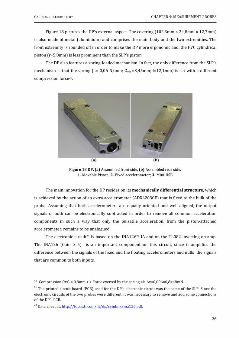
(a) (b)
Figure 18 DP. (a) Assembled front side. (b) Assembled rear side. 1- Movable Piston; 2- Fixed accelerometer; 3- Mini-USB
1 2
3
Figure 18 pictures the DP’s external aspect. The covering (102,3mm × 24,8mm × 12,7mm)
is also made of metal (aluminium) and comprises the main body and the two extremities. The
front extremity is rounded off in order to make the DP more ergonomic and, the PVC cylindrical
piston (r=5,0mm) is less prominent than the SLP’s piston.
The DP also features a spring-loaded mechanism. In fact, the only difference from the SLP’s
mechanism is that the spring (k= 0,06 N/mm; Øext =3,45mm; l=12,1mm) is set with a different
compression force20.
The main innovation for the DP resides on its mechanically differential structure, which
is achieved by the action of an extra accelerometer (ADXL203CE) that is fixed to the bulk of the
probe. Assuming that both accelerometers are equally oriented and well aligned, the output
signals of both can be electronically subtracted in order to remove all common acceleration
components in such a way that only the pulsatile acceleration, from the piston-attached
accelerometer, remains to be analogued.
The electronic circuit21 is based on the INA12622 IA and on the TL082 inverting op amp.
The INA126 (Gain ≥ 5) is an important component on this circuit, since it amplifies the
difference between the signals of the fixed and the floating accelerometers and nulls the signals
that are common to both inputs.
20 Compression (∆x) = 0,8mm ↔ Force exerted by the spring =k. ∆x=0,006×0,8=48mN. 21
The printed circuit board (PCB) used for the DP’s electronic circuit was the same of the SLP. Since the
electronic circuits of the two probes were different, it was necessary to remove and add some connections of the DP’s PCB. 22
Data sheet at: http://focus.ti.com/lit/ds/symlink/ina126.pdf.

CARDIOACCELEROMETERY CHAPTER 4: MEASUREMENT PROBES
27
As mentioned, the fixed and the floating accelerometers must be perfectly aligned and
with the same orientation, in order to guarantee the mechanically differential scheme. In this
way, the difference between their outputs will be zero when they have the same movement or
the probe is at rest.
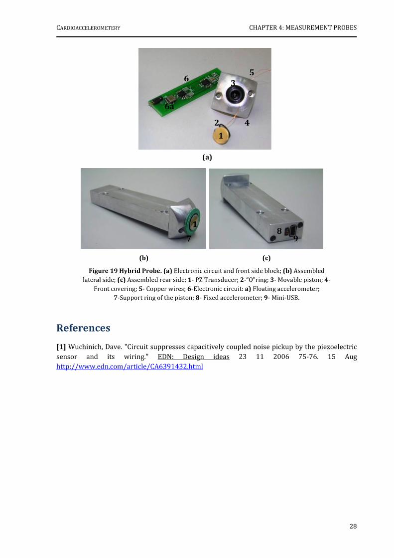
4.4 Hybrid Probe (HP)
The HP was the last version of the measurement probes to be developed. Although it has
not been tested in the clinical environment, it was tested in the pulsatory model (chapter 7).
This probe is an improved version of the DP, since it combines the spring-loaded and
differential mechanisms with an important source of information: a PZ transducer on the top of
the piston.
The placing of the PZ transducer on the piston implied some slightly changes in the
configuration of the probe, as is shown in figure 19.
The anterior extremity (25mm×25mm×12,8mm) of the metal covering23 is squared, with
rounded edges and presents an “o”ring that is attached to the PZ transducer, in order to improve
the adjustment of the tip to the acquisition location. The PZ signal is connected to the electronic
circuit by two enameled copper wires (signal and ground), that go through the piston and the
support piece.
The electronic circuit consists basically of the ADXL203 accelerometer, and the IAs, INA126
and INA121. The INA126, is set for a gain of 5 and, as in the DP, it amplifies the difference
between the accelerometer outputs. The INA12124, with unitary gain, suppresses the noise
pickup produced by the PZ transducer. Besides that, it presents current feedback via two
resistors of 8.2M, in order to eliminate guarding and achieve insulation requirements [1].
Appendix B shows a schematic that will allow a fully detailed understanding of the circuit.
23 Probes covering: 105,9mm×25mm×12,8mm.
24 Data sheet at: http://focus.ti.com/lit/ds/symlink/ina121.pdf.
CARDIOACCELEROMETERY CHAPTER 4: MEASUREMENT PROBES
28
(b) (c)
Figure 19 Hybrid Probe. (a) Electronic circuit and front side block; (b) Assembled lateral side; (c) Assembled rear side; 1- PZ Transducer; 2-“O”ring; 3- Movable piston; 4-
Front covering; 5- Copper wires; 6-Electronic circuit: a) Floating accelerometer; 7-Support ring of the piston; 8- Fixed accelerometer; 9- Mini-USB.
7
1 8
9
(a)
1
2
5
3
4
6
6a
References
[1] Wuchinich, Dave. "Circuit suppresses capacitively coupled noise pickup by the piezoelectric sensor and its wiring." EDN: Design ideas 23 11 2006 75-76. 15 Aug http://www.edn.com/article/CA6391432.html
29
CHAPTER 5
DAQ MODULES
As the measurement probes were being developed, it was also necessary to adjust the DAQ
module to their requirements.
Since five versions of the DAQ module were constructed to achieve this purpose, this
chapter depicts their principal features and successive improvements.
5.1 Introduction
The instrument enhancement involved not only the probe’s design upgrade but also the
development of a multichannel platform, which could integrate different hemodynamic signals.
In fact, the addition of different sensor types to the DAQ module came out from the need of
having several time references to allow accelerometric signal comprehension.
The first DAQ module version could only accommodate the SLP and the ECG sensors, in
opposite to the last one (fifth version) which already included the HP, the electrocardiograph,
two PZ transducers and one pressure sensor and an independent ±5V DC power supply.
Whether regarding the number of information channels or the signal to noise ratio (SNR)
at the output, each new version was actually better than the previous one.
5.2 Module A
As it is shown in figure 20, the first developed DAQ module comprised only an
electrocardiograph (to provide a starting time reference) and the NI USB-6008©.
The electrocardiograph circuit is based on the single-channel scheme described in section
2.5.3 and consequently it presents four electrodes which are placed on the body in agreement
with the configuration of lead I.
The analogue front-end (see circuit schematic at Appendix B) applies the typical approach
with an IA and a right leg common-mode feedback op amp. An AD62025 set to a gain of 9 is used
as IA and, a TL081 op amp is used to cancel the common mode interference. A variable gain
block follows, which allows for the adjustment of the output voltage signal, and a protection
25Data sheet at: http://www.analog.com/UploadedFiles/Data_Sheets/37793330023930AD620_e.pdf.

CARDIOACCELEROMETERY CHAPTER 5: DAQ MODULES
30
(a) (b)
Figure 20 DAQ Module A. (a) General view; (b) Inner side; 1- Electrocardiograph circuit; 2- NI USB-6008©.
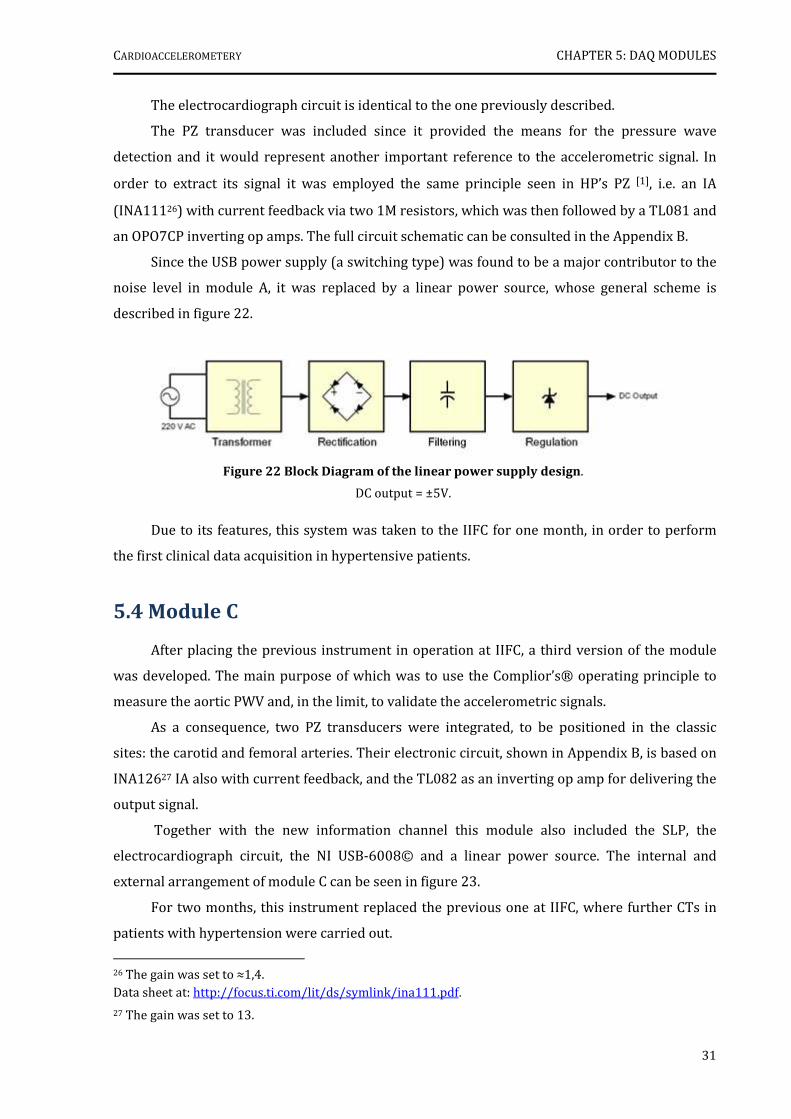
Figure 21 DAQ Module B.
1-Electrocardiograph circuit; 2- NI USB-6008©; 3-PZ amplification circuit; 4- Accelerometric probe’s input; 5-Power Supply.
1
2
3
4
5
5
block with back-biased diodes is placed on the signal path in order to provide protection from
over voltages. Power is supplied directly by the USB interface since the total current drawn by
the circuit is a fraction of the USB 500 mA limit.
Since the signals obtained with this module and the SLP presented high levels of noise, this
system was not used for CTs but only for lab trials.
5.3 Module B
A photograph of module B, the DAQ module’s second version, is shown in figure 21.
It contains not only three different information channels arising from the integration of
the SLP, the electrocardiograph circuit and one PZ transducer amplification circuit, but also the
NI DAQ-6008© and the power supply.
1 2
CARDIOACCELEROMETERY CHAPTER 5: DAQ MODULES
31
The electrocardiograph circuit is identical to the one previously described.
The PZ transducer was included since it provided the means for the pressure wave
detection and it would represent another important reference to the accelerometric signal. In
order to extract its signal it was employed the same principle seen in HP’s PZ [1], i.e. an IA
(INA11126) with current feedback via two 1M resistors, which was then followed by a TL081 and
an OPO7CP inverting op amps. The full circuit schematic can be consulted in the Appendix B.
Since the USB power supply (a switching type) was found to be a major contributor to the
noise level in module A, it was replaced by a linear power source, whose general scheme is
described in figure 22.
Due to its features, this system was taken to the IIFC for one month, in order to perform
the first clinical data acquisition in hypertensive patients.
5.4 Module C
After placing the previous instrument in operation at IIFC, a third version of the module
was developed. The main purpose of which was to use the Complior’s® operating principle to
measure the aortic PWV and, in the limit, to validate the accelerometric signals.
As a consequence, two PZ transducers were integrated, to be positioned in the classic
sites: the carotid and femoral arteries. Their electronic circuit, shown in Appendix B, is based on
INA12627 IA also with current feedback, and the TL082 as an inverting op amp for delivering the
output signal.
Together with the new information channel this module also included the SLP, the
electrocardiograph circuit, the NI USB-6008© and a linear power source. The internal and
external arrangement of module C can be seen in figure 23.
For two months, this instrument replaced the previous one at IIFC, where further CTs in
patients with hypertension were carried out.
26 The gain was set to ≈1,4. Data sheet at: http://focus.ti.com/lit/ds/symlink/ina111.pdf.
27 The gain was set to 13.
Figure 22 Block Diagram of the linear power supply design.
DC output = ±5V.

CARDIOACCELEROMETERY CHAPTER 5: DAQ MODULES
32
(a) (b)
Figure 23 DAQ Module C.
1-Electrocardiograph circuit; 2- NI USB-6008©; 3-PZ amplification circuit; 4- Power supply; 5-PZ Transducers; 6-SLP; 7-ECG electrodes.
1
2
3 4
4 5
6
7
Figure 24 DAQ Module D.
1- ECG’s input; 2- DP’s input; 3-PZ circuit.
2
3
1
5.5 Module D
The construction of the fourth DAQ module version, module D, was motivated by two
distinct needs: 1) to cope with the development of bench models on lab, which could simplify the
comprehension of clinical data; and, 2) the beginning of additional scientific research on PZ
based pulse wave assessment.
As is displayed in figure 24, this module reproduces the architecture of module C,
presenting the same three information channels (ECG, accelerometric and PZ), the NI USB-
6008® and the linear power source.
In fact, the only difference between them is the gain associated to the PZ circuit (GD=5)
which, in module C, was causing signal saturation due to its high value (GC=13).
For this reason this module and the recently made DP were taken to IIFC, where they have
been in operation acquiring data up to today.

CARDIOACCELEROMETERY CHAPTER 5: DAQ MODULES
33
Figure 25 DAQ Module E.
1- Pressure sensor’s input; 2- HP’s input
1 2
5.6 Module E
In order to accomplish all the requests
previously described, module C was slightly
modified, giving rise to the fifth and last DAQ
module version: module E (figure 25).
The first improvement had to do with
the gain of the PZ, which was adjusted to the
gain of module D. Besides, the two current
amplifiers INA126 were replaced by two
INA114.
The second upgrade consisted in the
insertion of a pressure acquisition channel that would be employed in the developed bench
models (see Chapter 7). The pressure sensor used was the HCXM100D6V28.
At last, the main similarities and differences between each module are resumed in table 5.
Table 5 Summary of the developed modules and its main features.
Features
Modules
Measurement
Probe
Incorporated
ECG No. of
Piezos Function Others
A SLP Trial Run Switching Power
Source (USB)
B SLP 1 CTs Linear Power Source
C SLP 2 CTs Linear Power Source
D DP 2 CTs Linear Power Source
E HP 2 Pulsatory Model Pressure Channel
Linear Power Source
References
[1] Wuchinich, Dave. "Circuit suppresses capacitively coupled noise pickup by the piezoelectric sensor and its wiring." EDN: Design ideas 23 11 2006 75-76. 15 Aug http://www.edn.com/article/CA6391432.html
28 Differential pressure range: 0-100mbar;
Data sheet at: http://www.lascarelectronics.com/DATA/sensor/HCX005D6V.pdf.
34
CHAPTER 6
ACCELEROMETER CALIBRATION
Prior to the clinical experiments with the differential probe, two bench models were
developed in order to help to interpret the clinical data.
The first model relates to the calibration of the accelerometer, while the second one has to
do with the simulation of a pulsatory system for the full understanding of the relationship
between accelerometric, PZ and pressure signals (Chapter 7).
This chapter focuses only the calibration of the accelerometer, firstly by describing the
experimental set-up and, afterwards, by interpreting the obtained results.
6.1 Introduction
As mentioned in chapter 2, the calibration process consists in applying an excitation or a
reference signal of known mechanical characteristics and measuring the subsequent electrical
output of the sensor/instrument under test [1].
To achieve this goal, we made an option of building a slider-crank mechanism (SCM), due
to its simplicity and ease of construction. Through this reference apparatus, a sinusoidal-like
motion, with variable frequencies and amplitudes is produced to measure the ADXL203
accelerometer output.
In order to understand the basic concepts of a SCM, the next subsection is entirely devoted
to its mathematical description.
6.1.1 Slider-Crank Mechanism
The SC mechanism is an arrangement of mechanical parts designed to convert rotary
motion to straight-line motion or vice-versa.
The basic nature of the mechanism and the relative motion of the parts can be best
described with the help of figure 26.
The darkly shaded part 1 corresponds to the cylinder29, in which the piston or slider (part
4) slides back and forth. The crank, part 2, is shown as a straight line member extending from
29 Or two guides.
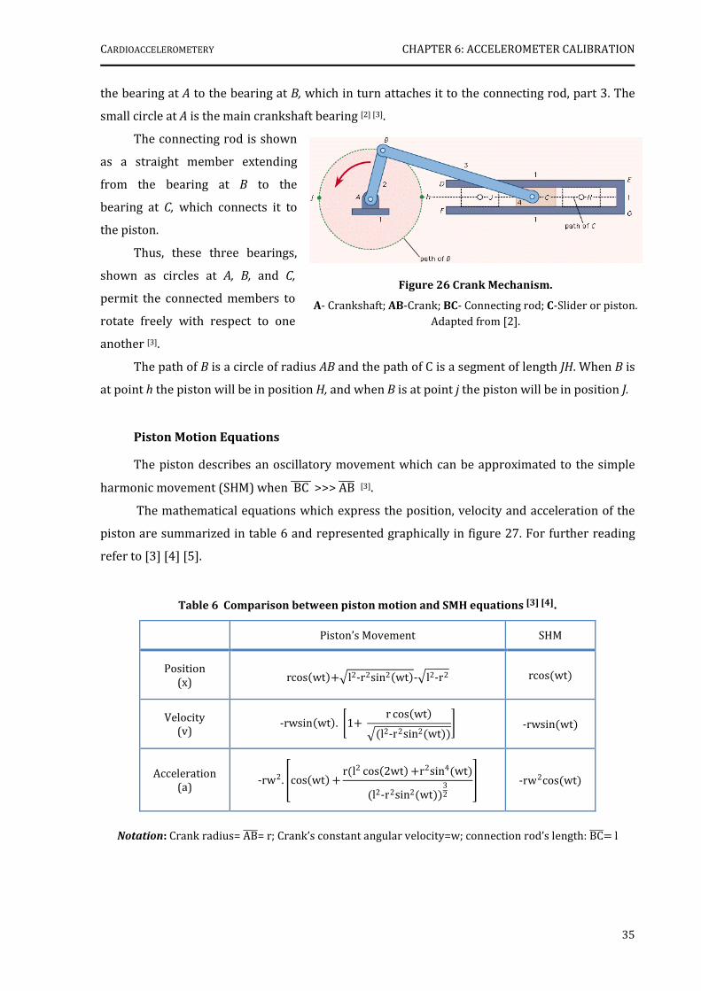
CARDIOACCELEROMETERY CHAPTER 6: ACCELEROMETER CALIBRATION
35
the bearing at A to the bearing at B, which in turn attaches it to the connecting rod, part 3. The
small circle at A is the main crankshaft bearing [2] [3].
The connecting rod is shown
as a straight member extending
from the bearing at B to the
bearing at C, which connects it to
the piston.
Thus, these three bearings,
shown as circles at A, B, and C,
permit the connected members to
rotate freely with respect to one
another [3].
The path of B is a circle of radius AB and the path of C is a segment of length JH. When B is
at point h the piston will be in position H, and when B is at point j the piston will be in position J.
Piston Motion Equations
The piston describes an oscillatory movement which can be approximated to the simple
harmonic movement (SHM) when BC ----- >>> AB---- [3].
The mathematical equations which express the position, velocity and acceleration of the
piston are summarized in table 6 and represented graphically in figure 27. For further reading
refer to [3] [4] [5].
Table 6 Comparison between piston motion and SMH equations [3] [4].
Piston’s Movement SHM
Position (x) rcoswt (0l2‐r2sin2wt ‐0l2‐r2 rcoswt
Velocity (v)
‐rwsinwt . 51( r coswt 0l2‐r2sin2wt 7 ‐rwsinwt
Acceleration (a) ‐rw2. 8coswt ( rl2 cos2wt (r2sin4wt
l2‐r2sin2wt 32 ; ‐rw2coswt
Notation: Crank radius= AB----= r; Crank’s constant angular velocity=w; connection rod’s length: BC---- l
Figure 26 Crank Mechanism.
A- Crankshaft; AB-Crank; BC- Connecting rod; C-Slider or piston.
Adapted from [2].
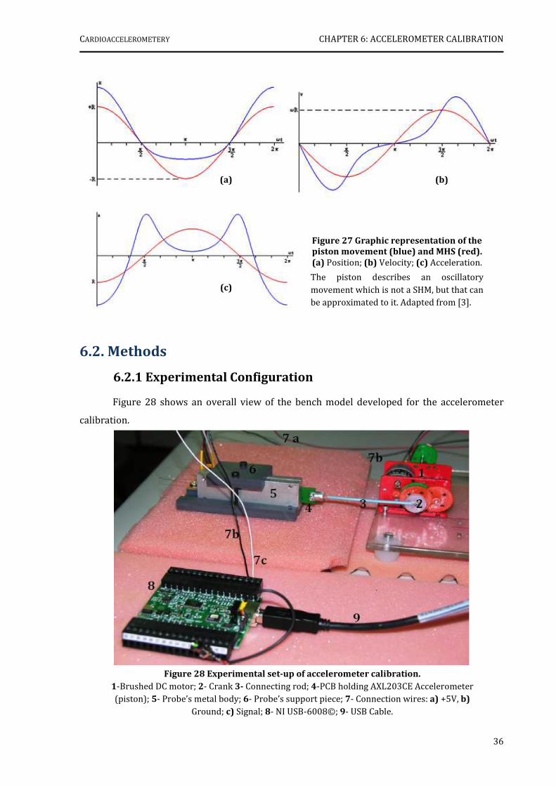
CARDIOACCELEROMETERY CHAPTER 6: ACCELEROMETER CALIBRATION
36
6.2. Methods
6.2.1 Experimental Configuration
Figure 28 shows an overall view of the bench model developed for the accelerometer
calibration.
(a) (b)
(c)
Figure 27 Graphic representation of the
piston movement (blue) and MHS (red).
(a) Position; (b) Velocity; (c) Acceleration.
The piston describes an oscillatory
movement which is not a SHM, but that can be approximated to it. Adapted from [3].
Figure 28 Experimental set-up of accelerometer calibration.
1-Brushed DC motor; 2- Crank 3- Connecting rod; 4-PCB holding AXL203CE Accelerometer (piston); 5- Probe’s metal body; 6- Probe’s support piece; 7- Connection wires: a) +5V, b)
Ground; c) Signal; 8- NI USB-6008©; 9- USB Cable.
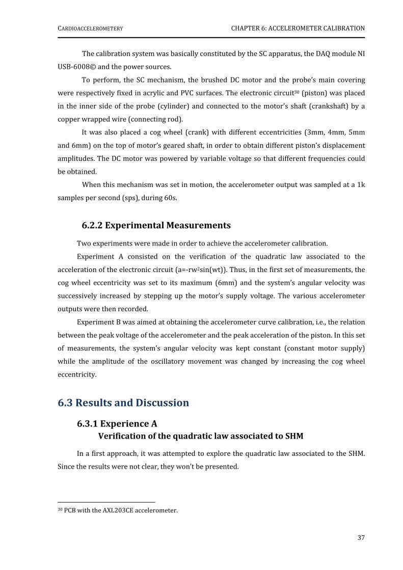
CARDIOACCELEROMETERY CHAPTER 6: ACCELEROMETER CALIBRATION
37
The calibration system was basically constituted by the SC apparatus, the DAQ module NI
USB-6008© and the power sources.
To perform, the SC mechanism, the brushed DC motor and the probe’s main covering
were respectively fixed in acrylic and PVC surfaces. The electronic circuit30 (piston) was placed
in the inner side of the probe (cylinder) and connected to the motor’s shaft (crankshaft) by a
copper wrapped wire (connecting rod).
It was also placed a cog wheel (crank) with different eccentricities (3mm, 4mm, 5mm
and 6mm) on the top of motor’s geared shaft, in order to obtain different piston’s displacement
amplitudes. The DC motor was powered by variable voltage so that different frequencies could
be obtained.
When this mechanism was set in motion, the accelerometer output was sampled at a 1k
samples per second (sps), during 60s.
6.2.2 Experimental Measurements
Two experiments were made in order to achieve the accelerometer calibration.
Experiment A consisted on the verification of the quadratic law associated to the
acceleration of the electronic circuit (a=-rw2sin(wt)). Thus, in the first set of measurements, the
cog wheel eccentricity was set to its maximum (6mm) and the system’s angular velocity was
successively increased by stepping up the motor’s supply voltage. The various accelerometer
outputs were then recorded.
Experiment B was aimed at obtaining the accelerometer curve calibration, i.e., the relation
between the peak voltage of the accelerometer and the peak acceleration of the piston. In this set
of measurements, the system’s angular velocity was kept constant (constant motor supply)
while the amplitude of the oscillatory movement was changed by increasing the cog wheel
eccentricity.
6.3 Results and Discussion
6.3.1 Experience A
Verification of the quadratic law associated to SHM
In a first approach, it was attempted to explore the quadratic law associated to the SHM.
Since the results were not clear, they won’t be presented.
30 PCB with the AXL203CE accelerometer.
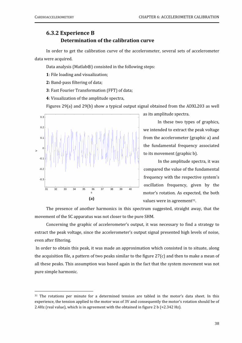
CARDIOACCELEROMETERY CHAPTER 6: ACCELEROMETER CALIBRATION
38
31 32 33 34 35 36 37 38 39 40
-0.3
-0.2
-0.1
0
0.1
0.2
0.3
s
V
(a)
6.3.2 Experience B
Determination of the calibration curve
In order to get the calibration curve of the accelerometer, several sets of accelerometer
data were acquired.
Data analysis (Matlab®) consisted in the following steps:
1: File loading and visualization;
2: Band-pass filtering of data;
3: Fast Fourier Transformation (FFT) of data;
4: Visualization of the amplitude spectra,
Figures 29(a) and 29(b) show a typical output signal obtained from the ADXL203 as well
as its amplitude spectra.
In these two types of graphics,
we intended to extract the peak voltage
from the accelerometer (graphic a) and
the fundamental frequency associated
to its movement (graphic b).
In the amplitude spectra, it was
compared the value of the fundamental
frequency with the respective system’s
oscillation frequency, given by the
motor’s rotation. As expected, the both
values were in agreement31.
The presence of another harmonics in this spectrum suggested, straight away, that the
movement of the SC apparatus was not closer to the pure SHM.
Concerning the graphic of accelerometer’s output, it was necessary to find a strategy to
extract the peak voltage, since the accelerometer’s output signal presented high levels of noise,
even after filtering.
In order to obtain this peak, it was made an approximation which consisted in to situate, along
the acquisition file, a pattern of two peaks similar to the figure 27(c) and then to make a mean of
all these peaks. This assumption was based again in the fact that the system movement was not
pure simple harmonic.
31 The rotations per minute for a determined tension are tabled in the motor’s data sheet. In this experience, the tension applied to the motor was of 3V and consequently the motor’s rotation should be of
2.4Hz (real value), which is in agreement with the obtained in figure 2 b (≈2.342 Hz).
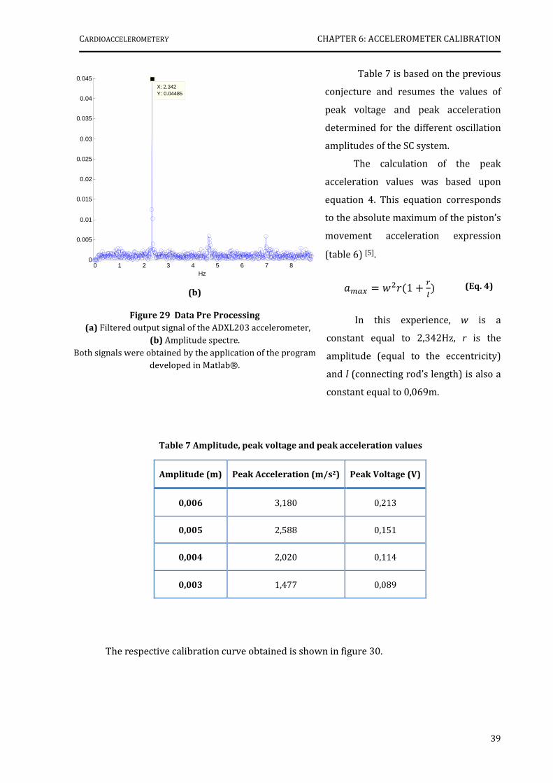
CARDIOACCELEROMETERY CHAPTER 6: ACCELEROMETER CALIBRATION
39
(b)
Figure 29 Data Pre Processing
(a) Filtered output signal of the ADXL203 accelerometer, (b) Amplitude spectre.
Both signals were obtained by the application of the program developed in Matlab®.
0 1 2 3 4 5 6 7 80
0.005
0.01
0.015
0.02
0.025
0.03
0.035
0.04
0.045X: 2.342Y: 0.04485
Hz
Table 7 is based on the previous
conjecture and resumes the values of
peak voltage and peak acceleration
determined for the different oscillation
amplitudes of the SC system.
The calculation of the peak
acceleration values was based upon
equation 4. This equation corresponds
to the absolute maximum of the piston’s
movement acceleration expression
(table 6) [5].
<=> ?@A1 ( BC
In this experience, w is a
constant equal to 2,342Hz, r is the
amplitude (equal to the eccentricity)
and l (connecting rod’s length) is also a
constant equal to 0,069m.
Table 7 Amplitude, peak voltage and peak acceleration values
Amplitude (m) Peak Acceleration (m/s2) Peak Voltage (V)
0,006 3,180 0,213
0,005 2,588 0,151
0,004 2,020 0,114
0,003 1,477 0,089
The respective calibration curve obtained is shown in figure 30.
(Eq. 4)
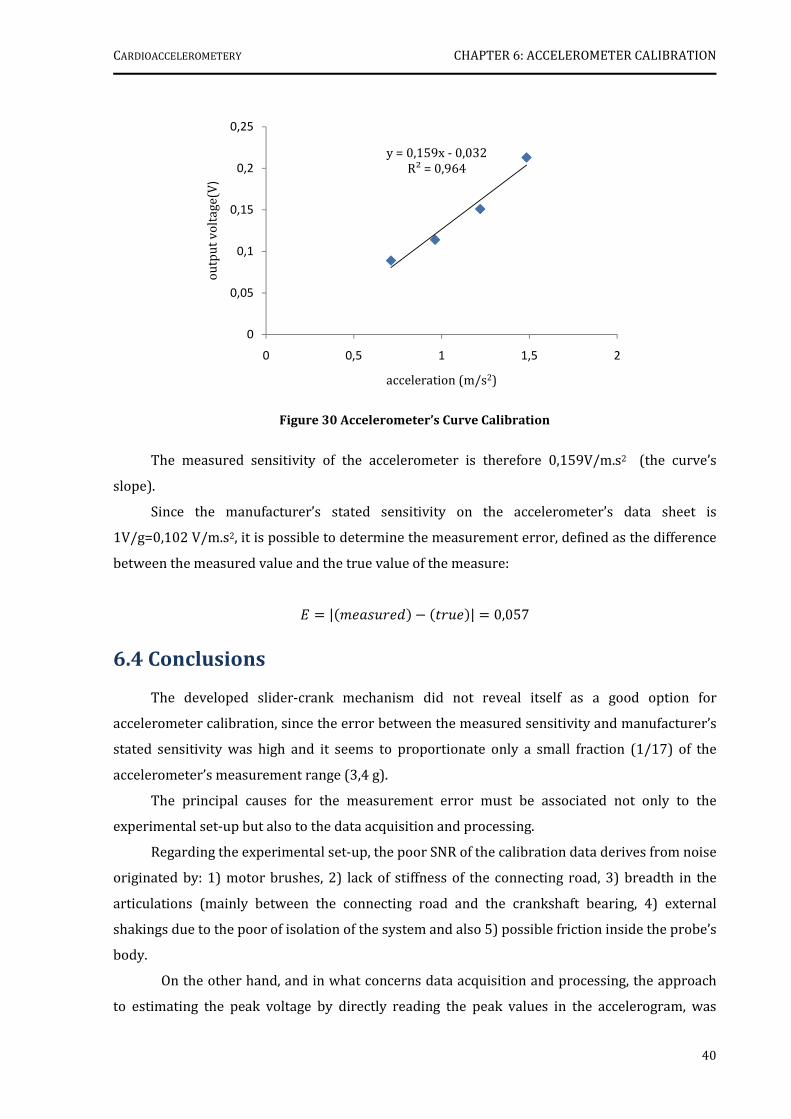
CARDIOACCELEROMETERY CHAPTER 6: ACCELEROMETER CALIBRATION
40
Figure 30 Accelerometer’s Curve Calibration
The measured sensitivity of the accelerometer is therefore 0,159V/m.s2 (the curve’s
slope).
Since the manufacturer’s stated sensitivity on the accelerometer’s data sheet is
1V/g=0,102 V/m.s2, it is possible to determine the measurement error, defined as the difference
between the measured value and the true value of the measure:
|EFGAEH " IAGE | 0,057
6.4 Conclusions
The developed slider-crank mechanism did not reveal itself as a good option for
accelerometer calibration, since the error between the measured sensitivity and manufacturer’s
stated sensitivity was high and it seems to proportionate only a small fraction (1/17) of the
accelerometer’s measurement range (3,4 g).
The principal causes for the measurement error must be associated not only to the
experimental set-up but also to the data acquisition and processing.
Regarding the experimental set-up, the poor SNR of the calibration data derives from noise
originated by: 1) motor brushes, 2) lack of stiffness of the connecting road, 3) breadth in the
articulations (mainly between the connecting road and the crankshaft bearing, 4) external
shakings due to the poor of isolation of the system and also 5) possible friction inside the probe’s
body.
On the other hand, and in what concerns data acquisition and processing, the approach
to estimating the peak voltage by directly reading the peak values in the accelerogram, was
y = 0,159x - 0,032R² = 0,964
0
0,05
0,1
0,15
0,2
0,25
0 0,5 1 1,5 2
outp
ut
volt
age(
V)
acceleration (m/s2)
CARDIOACCELEROMETERY CHAPTER 6: ACCELEROMETER CALIBRATION
41
probably not adequate, since it is subjective. Thus, the future utilization of this mechanism in
accelerometer calibration would necessarily imply an optimization of the experimental
configuration, in order to obtain higher SNR, and would also require second thoughts on data
processing methods. Eventually, the exploitation of the singularities of the spectral properties of
functions xx, yy , will lead to interesting results.
References
[1] Webster, John G., Measurement, Instrumentation and Sensors Handbook, 1st ed. New York: CRC Press LLC, 1999, pp:
[2] “Slider-crank mechanism." Online Art. Encyclopædia Britannica Online. 3 Sept. 2007 http://www.britannica.com/eb/art-7447
[3] García, Ángel. "Movimiento de un pistón." Física con ordenador. 3 Oct 2006. 2 Sep 2007 http://www.sc.ehu.es/sbweb/fisica/oscilaciones/biela/biela.htm
[4] "Piston motion equations." 7 Jul 2007. Wikipedia. 2 Sep 2007 http://en.wikipedia.org/wiki/Piston_motion_equations
[5] Santos, António, “Introdução aos motores de combustão interna” , Class Notes, pp.15-17
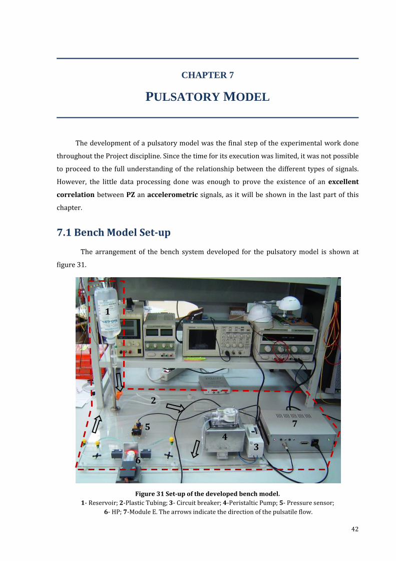
42
Figure 31 Set-up of the developed bench model.
1- Reservoir; 2-Plastic Tubing; 3- Circuit breaker; 4-Peristaltic Pump; 5- Pressure sensor;
6- HP; 7-Module E. The arrows indicate the direction of the pulsatile flow.
1
2
3 4
5 7
6
CHAPTER 7
PULSATORY MODEL
The development of a pulsatory model was the final step of the experimental work done
throughout the Project discipline. Since the time for its execution was limited, it was not possible
to proceed to the full understanding of the relationship between the different types of signals.
However, the little data processing done was enough to prove the existence of an excellent
correlation between PZ an accelerometric signals, as it will be shown in the last part of this
chapter.
7.1 Bench Model Set-up
The arrangement of the bench system developed for the pulsatory model is shown at
figure 31.

CARDIOACCELEROMETERY CHAPTER 7: PULSATORY MODEL
43
The pulsatory model is divided in two main parts: the fluid circulation circuit and the DAQ
system.
The fluid circulation circuit is fixed on an acrylic surface and is constituted by plastic
tubes, a water reservoir (500 ml), a peristaltic pump (PP)32 and a 10 mA differential circuit
breaker, which protects the operator from over load or short circuit, and powers up motor
pump. The PP establishes a water pulsatile flow of 5l/h in the direction of the arrows, as the
figure points out.
The DAQ system comprises the HP, the HCXM100D6V differential pressure sensor and the
module E. The HP, horizontally fixed with an appropriate holder, is leaned against a rubber
elastic membrane. The need to glue an elastic membrane on the plastic tube is due to its
stiffness, which would make difficult the signal acquisition. Previously to gluing the rubber
elastic membrane to the tube a partial small cut have to be done.
7.2 Results
With the configuration described before it was possible to acquire accelerometric, PZ and
pressure signals, simultaneously.
In figure 32 is shown the typical signals obtained during 4s, using an acquisition sample
rate of 1ksps. These signals were already filtered in Matlab® with a band-pass filter of [0.4 Hz,
45 Hz].
7.3 Data Processing
The acquired signals suffered a very superficial data processing treatment, however, and
having in mind to find a relationship between the patterns recognized for each signal, the
accelerometric and PZ signals were compared.
It was developed a small algorithm which consisted in the following main steps and whose
final result is presented in figures 33(a) and 33(b):
Step 1: File load and visualization;
Step 2: Filtering: application of a band-pass filter [0.4 Hz, 45 Hz];
Step 3: Double differentiation of the PZ signal;
Step 4: Normalization of the accelerometric and the differentiate PZ, signals;
Step 5: Simultaneous visualization of the normalized signals. 32 A peristaltic pump is a type of positive displacement pump (compression pump) used for pumping a
variety of fluids. The fluid is contained within a flexible silicon tube fitted inside the circular pump casing.
A rotor, with a determined number of rollers, compresses the flexible tube in order to produce the flow. For further reading: http://en.wikipedia.org/wiki/Peristaltic_pump2
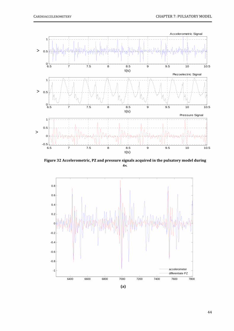
CARDIOACCELEROMETERY CHAPTER 7: PULSATORY MODEL
44
6.5 7 7.5 8 8.5 9 9.5 10 10.50
0.5
1
t(s)
VAccelerometric Signal
6.5 7 7.5 8 8.5 9 9.5 10 10.50
0.5
1
t(s)
V
Piezoelectric Signal
6.5 7 7.5 8 8.5 9 9.5 10 10.5-0.5
0
0.5
1
t(s)
V
Pressure Signal
6400 6600 6800 7000 7200 7400 7600 7800
-1
-0.8
-0.6
-0.4
-0.2
0
0.2
0.4
0.6
0.8
accelerometer
differentiate PZ
(a)
Figure 32 Accelerometric, PZ and pressure signals acquired in the pulsatory model during
4s.

CARDIOACCELEROMETERY CHAPTER 7: PULSATORY MODEL
45
6350 6400 6450 6500 6550 6600 6650
-1
-0.5
0
0.5
1
accelerometer
differentiate PZ
It is observed an explicit correlation between the shapes of both signals. Thus, it is proved
that the accelerometer gives, at least, the same information as the PZ when it is differentiated
twice. In fact, we suppose that the information provided by the accelerometer can be more
valuable that those obtained directly by the PZ, since PZ is inherently an AC coupled device and,
as such, its frequency response always depends on the time constant of the overall circuit, and it
is inevitably impaired in the very low range (DC to 0.2 Hz), where a number of auto-regulatory
effects of the human body, are located [1].
Moreover, even for the frequencies where the response is not affected by the coupling (0.2
Hz up to resonance), the response delivered by PZ is affected by the way the operator holds the
probe and presses it against the region under test (this is the reason why the HP has been fixed
in this model). This uncertainty is due to the complex relationship between charge polarization
and externally applied forces in the bulk of the sensor material.
For these reasons PZs cannot be calibrated in terms of a mechanical unit (pressure, force,
torque or other) against output voltage. In fact all hemodynamic instruments using PZs are used
for time measurements, only.
Accelerometers, on the contrary, are truly DC devices capable of a complete 3-axis
assessment of a precise mechanical parameter, and when incorporated in a well designed probe,
many artefacts, associated to the operator involuntary movements, can be eliminated.
References
[1] Humeau, Anne. et al, Numerical Simulation of Laser Doppler Flowmetry Signals Based on a Model of Nonlinear Coupled Oscillators. Comparison with Real Data in the Frequency Domain (I), Proceedings of the 29th Annual International Conference of the IEEE EMBS, pp. 4068-4071.
(b)
Figure 33 Accelerometric and Double Differentiate PZ Signals:
(a) General view. (b) Peak amplification.
46
CHAPTER 8
CLINICAL RESEARCH TESTS
This final chapter describes the procedures of the CTs carried out in IIFC, and establishes a
comparison between the data acquired with the various probes/modules.
8.1 CTs Procedures
As mentioned before, the second period of CTs was carried out respectively by: the
SLP/module B (1 month), the SLP/module C (2 months) and the DP/module D (in still progress).
The clinical trials main objective is to explore the potential of the accelerometer based
probes in the assessment of PWV, by comparing their information with the one of a standard
method (Complior®). Since the DAQ modules C and D incorporate a similar (and inexpensive)
input, based on a principle similar to the Complior’s®, it is also intended to investigate the
feasibility of extracting transit time curves with this platform, to further PWV computing.
The type-of-patient criteria of selection changed in relation to the first period (section
3.3.1): currently, all patients are hypertensive and have been submitted to drug treatment. This
circumstance makes it possible a valuable comparison of PWV values, before and after
medication.
The three types of acquisitions performed are summarized in table 8.
Table 8 Acquisition types performed with the various probes/modules.
(It was used the Complior® to perform a 4th test, in order to obtain the PWV real value).
Acquisition Type Description
Probe + ECG After the ECG sensors are located in agreement with lead I
configuration, the operator places the measurement probe over the carotid artery, during 30-45s.
Probe + PZ Two operators place the probe and the PZ, respectively, in opposition
over the carotid arteries, during 30s-45s.
PZ + PZ1 The operator places the PZs over carotid and femoral arteries during
15 s, approximately.
1The PZ+PZ CT was not performed by the SLP/module B.

CARDIOACCELEROMETERY CHAPTER 8: CLINICAL RESEARCH TESTS
47
0.5 1 1.5 2 2.5 3 3.5
-0.8
-0.6
-0.4
-0.2
0
0.2
0.4
0.6
0.8
t(s)
V
ECG
Accel
2 2.5 3 3.5 4 4.5 5 5.5
-4
-3
-2
-1
0
1
2
3
t(s)
V
PZ
Accel
8.2 Data Pre-Processing
Up to now, data from nearly forty patients have been subject to the clinical trials and some
of them are now entering the second turn of evaluation.
However, and since the project’s priority was hardware optimization in order to obtain
signals with high SNR, the acquired data has not yet been processed, in an attempt to relate
them with the Complior’s® information. In fact, so far, the data pre-processing that was carried
out (data visualization and filtering) has been used for the instrument improvement, only.
Next, some representative examples are shown in order to compare signals obtained with
the different instrument set-ups (figures 34, 35 and 36).
1) SLP/Module B
Figure 34 Signals acquired by the SLP/Module B in one patient.
(a) ECG+Accelerometer. (b) ECG+PZ.
(a)
(b)
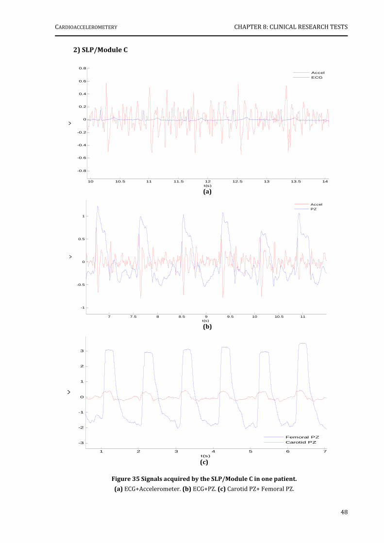
CARDIOACCELEROMETERY CHAPTER 8: CLINICAL RESEARCH TESTS
48
10 10.5 11 11.5 12 12.5 13 13.5 14
-0.8
-0.6
-0.4
-0.2
0
0.2
0.4
0.6
0.8
t(s)
V
Accel
ECG
7 7.5 8 8.5 9 9.5 10 10.5 11
-1
-0.5
0
0.5
1
t(s)
V
Accel
PZ
2) SLP/Module C
1 2 3 4 5 6 7
-3
-2
-1
0
1
2
3
t(s)
V
Femoral PZ
Carotid PZ
Figure 35 Signals acquired by the SLP/Module C in one patient.
(a) ECG+Accelerometer. (b) ECG+PZ. (c) Carotid PZ+ Femoral PZ.
(a)
(b)
(c)
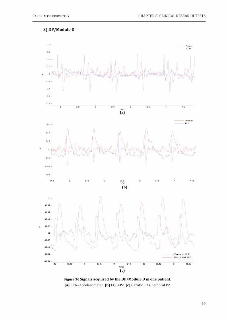
CARDIOACCELEROMETERY CHAPTER 8: CLINICAL RESEARCH TESTS
49
1 1.5 2 2.5 3 3.5 4 4.5
-0.8
-0.6
-0.4
-0.2
0
0.2
0.4
0.6
0.8
t(s)
V
Accel
ECG
5 5.5 6 6.5 7 7.5 8 8.5 9 9.5-0.8
-0.6
-0.4
-0.2
0
0.2
0.4
0.6
0.8
1
t(s)
V
Carotid PZ
Femoral PZ
(c)
0.5 1 1.5 2 2.5 3 3.5 4 4.5
-0.6
-0.4
-0.2
0
0.2
0.4
0.6
t(s)
V
Accel
PZ
3) DP/Module D
(b)
(a)
Figure 36 Signals acquired by the DP/Module D in one patient.
(a) ECG+Accelerometer. (b) ECG+PZ. (c) Carotid PZ+ Femoral PZ.

CARDIOACCELEROMETERY CHAPTER 8: CLINICAL RESEARCH TESTS
50
It is quite clear that the accelerometric and PZ signals acquired with the DP/module D set-
up exhibit higher SNR than those obtained with the other probe/modules set-ups, and the
observed saturation on PZ signals has disappeared also when using this set-up. In fact, the only
signals whose SNR is constant throughout the use of different set-ups are the ECG ones.
Although the pre-processing of the clinical data is not enough to conclude the exact
information values that the accelerometer is able to give, the existence of very well defined
correlations between the different signals is also very clear, thus making it an interesting subject
for further research.
51
CHAPTER 9
CONCLUSIONS AND FUTURE WORK
Once the project’s academic component has been achieved, it is now necessary to
evaluate and discuss the work that has been done, the results obtained and the future
developments.
9.1 Conclusions
The main objective of this project was the development of instrumental methods, based in
accelerometery, for PWV hemodynamic characterization.
Three accelerometer based probes (SLP, DP and HP) and five multisensor DAQ modules
(A, B, C, D and E) were designed and built for this purpose and have been tested in the field.
In its research usage, they have proved effective in the prolonged follow up of
hypertensive patients and, at this point, the instrument with the better performance is the DP
and module D, which exhibit signals with a higher SNR.
The pre-processing of the clinical data was not conclusive about the exact information that
accelerometer was able to give, but the existence of very well defined correlations between the
ECG, accelerometric and PZ signals suggests a high potential for this new technique.
In order to help the comprehension of the clinical data, two bench models were also
developed. The first addresses the calibration of the ADXL203 accelerometer. Although the
simplicity of the mechanism was very attractive, the device was only capable of testing a small
fraction of the accelerometer’s measurement range. In addition, the difference between the
measured sensitivity and manufacturer’s stated sensitivity was extremely high.
The second model had to do with the simulation of a pulsatory model. The analysis of the
signals acquired with the HP revealed that the accelerometer delivers, at least, the same
information as the PZ when its output curve is differentiated twice.
In the future, it is expected that the best performance in clinical trials would be from the
HP or from a similar version, which, in the limit, will be able to compute PWV punctually in the
carotid artery.
CARDIOACCELEROMETERY CHAPTER 9: CONCLUSIONS AND FUTURE WORK
52
9.2 Future work
In this work, the feasibility of using accelerometers in the assessment of PWV was
explored and the results obtained with prototype probes were indeed very promising.
However, there is still much work to be done in order to achieve a powerful and reliable
instrument for hemodynamic characterization of PWV, and to turn this technique into a
marketable technology.
Since this project is to be continued, the two main steps which are necessary to take in
the short term are related not only to the instrument itself but to the clinical data processing.
Instrument Optimisation
Since they two major limitations on the performance of NI-DAQ 6008 © were found
(software inflexibility and reduced real time capacities), it will be necessary to develop an
electronic platform with real time signal analysis capacity. The integration of a late generation
microcontroller as the unit’s core will be the best solution.
The analog front end should maintain the current number of channels (accelerometric
probe, PZ transducers, electrocardiograph circuit), but must have a modular structure to allow
simple adaptations in order to add other sensors of interest (temperature, oximetry…). As for
the communication with the PC, although not critical, it should be done by means of a standard
RF communication protocol (Zigbee, Bluetooth...), in order to guarantee connectivity and
portability.
The validation of this platform will be made with the clinical tests extension.
Clinical data Processing
Undoubtedly, clinical data processing is the key to the major goals of this work. It will
remove the obstacles found in the assessment of PWV values obtained by accelerometery, and
will enable a comprehensive comparison with Complior’s® data.
Ultimately, it will be data processing that will lead the way to the validation of a clinical
instrument based on the new (to our knowledge) techniques unveiled in this work.
To attain this goal, it will be necessary, firstly, to study the relationship between the
different signals in an ideal model and, then, bring the data processing, already started for the
pulsatory model, to a conclusion.
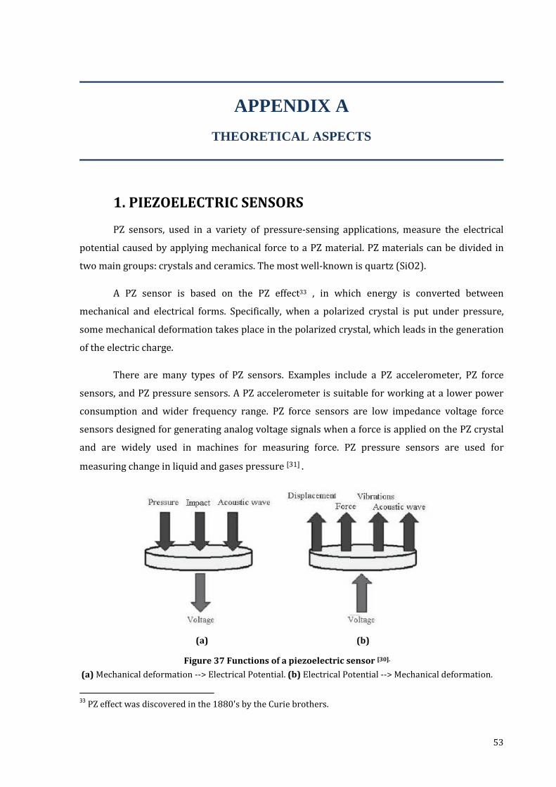
53
APPENDIX A
THEORETICAL ASPECTS
1. PIEZOELECTRIC SENSORS
PZ sensors, used in a variety of pressure-sensing applications, measure the electrical
potential caused by applying mechanical force to a PZ material. PZ materials can be divided in
two main groups: crystals and ceramics. The most well-known is quartz (SiO2).
A PZ sensor is based on the PZ effect33 , in which energy is converted between
mechanical and electrical forms. Specifically, when a polarized crystal is put under pressure,
some mechanical deformation takes place in the polarized crystal, which leads in the generation
of the electric charge.
There are many types of PZ sensors. Examples include a PZ accelerometer, PZ force
sensors, and PZ pressure sensors. A PZ accelerometer is suitable for working at a lower power
consumption and wider frequency range. PZ force sensors are low impedance voltage force
sensors designed for generating analog voltage signals when a force is applied on the PZ crystal
and are widely used in machines for measuring force. PZ pressure sensors are used for
measuring change in liquid and gases pressure [31] .
33
PZ effect was discovered in the 1880's by the Curie brothers.
(a) (b)
Figure 37 Functions of a piezoelectric sensor [30].
(a) Mechanical deformation --> Electrical Potential. (b) Electrical Potential --> Mechanical deformation.

APPENDIX A
54
2. ELECTROCARDIOGRAPHY
Heart’s Anatomy
The next figure is a sketch of the heart, showing its main structures and arterial and
venous connections:
12-Lead Placement Diagrams
The 12-lead ECG provides spatial information about the heart's electrical activity. The
three standard limb leads (I, II, III) and the augmented limb leads (aVR, aVL, aVF) detect the
electrical potential change in the frontal plane. The six precordial leads (V1,V2,V3,V4,V5,V6), each
in a different position along the chest, record the electric potential change in the heart in a cross
sectional plane. The diagrams below illustrate the location of the electrodes for each lead.
Figure 38 The Heart. Adapted from [25].
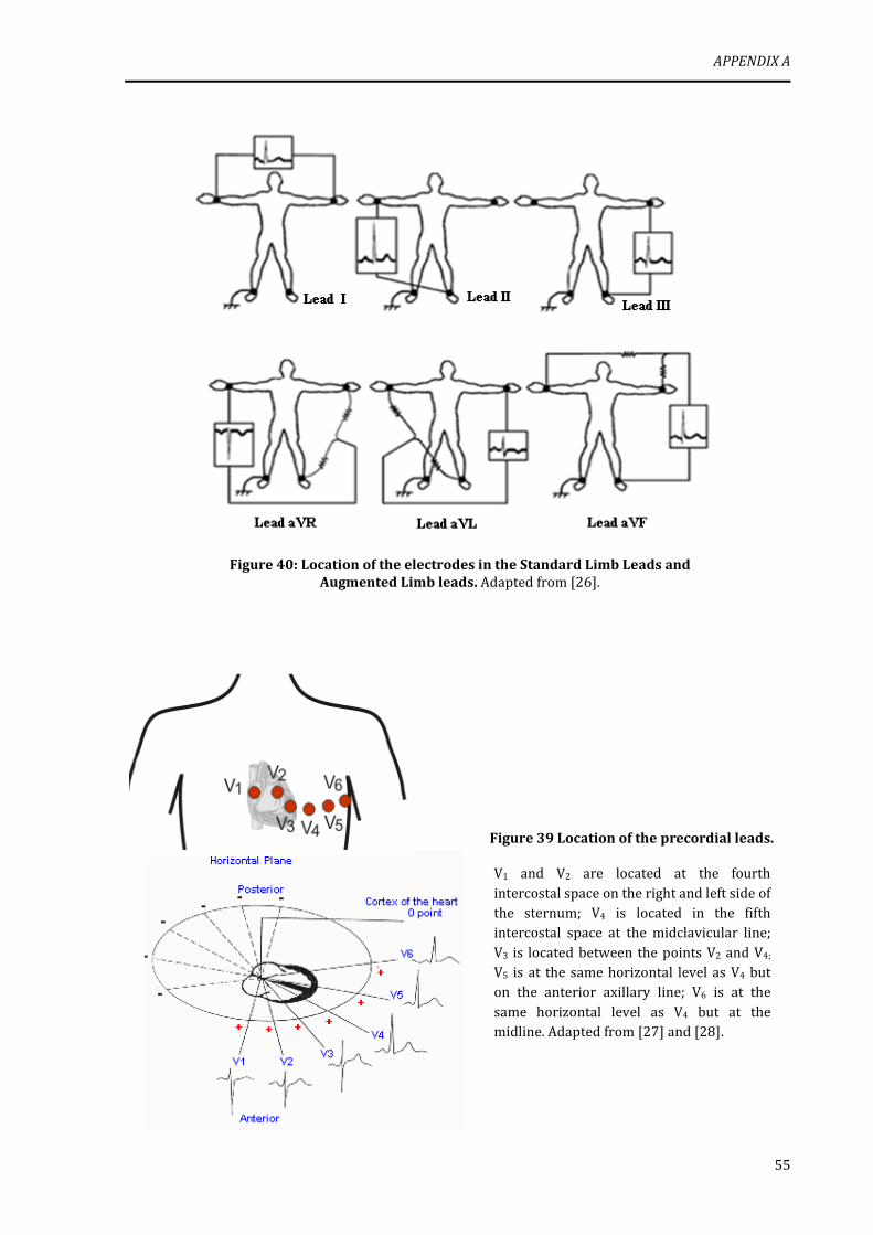
APPENDIX A
55
Figure 40: Location of the electrodes in the Standard Limb Leads and
Augmented Limb leads. Adapted from [26].
Figure 39 Location of the precordial leads.
V1 and V2 are located at the fourth
intercostal space on the right and left side of the sternum; V4 is located in the fifth intercostal space at the midclavicular line;
V3 is located between the points V2 and V4;
V5 is at the same horizontal level as V4 but on the anterior axillary line; V6 is at the
same horizontal level as V4 but at the midline. Adapted from [27] and [28].
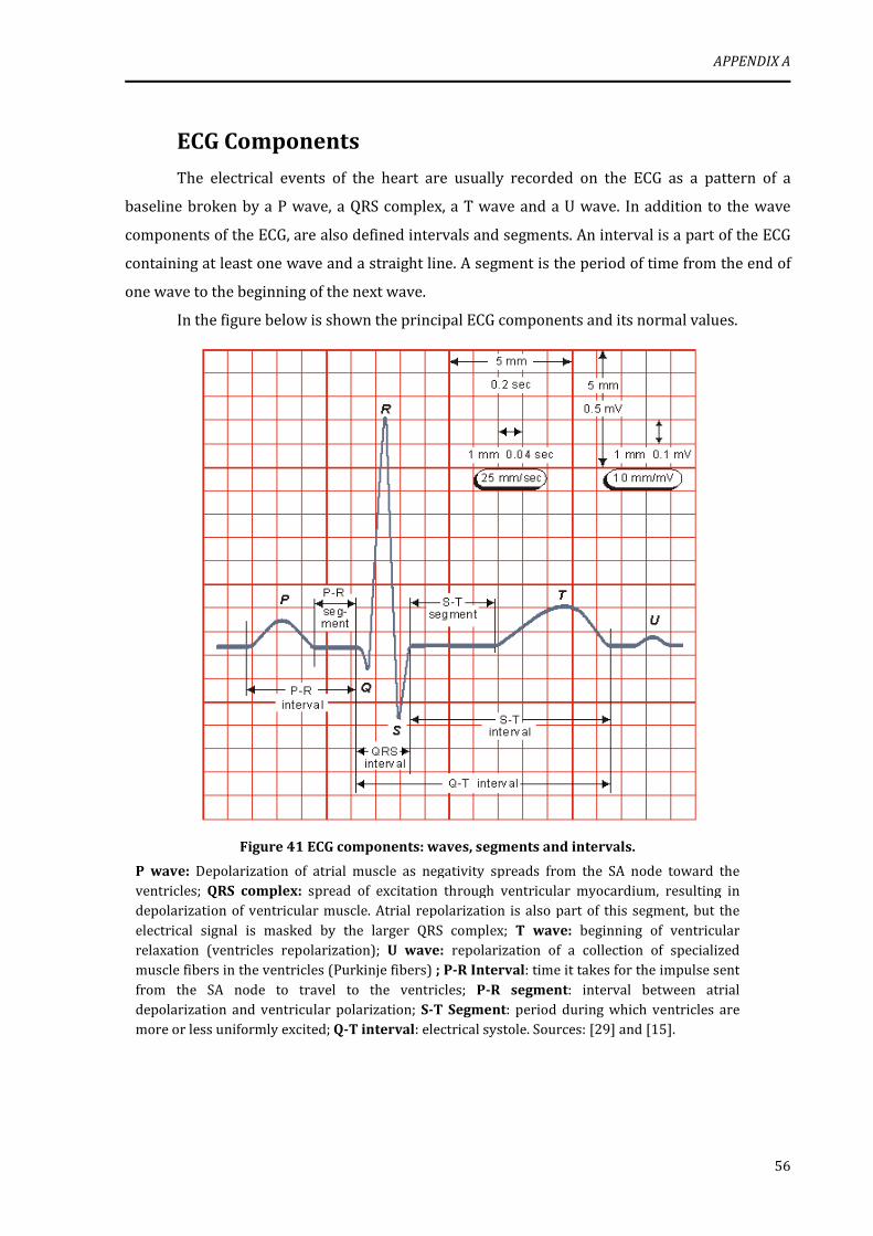
APPENDIX A
56
ECG Components
The electrical events of the heart are usually recorded on the ECG as a pattern of a
baseline broken by a P wave, a QRS complex, a T wave and a U wave. In addition to the wave
components of the ECG, are also defined intervals and segments. An interval is a part of the ECG
containing at least one wave and a straight line. A segment is the period of time from the end of
one wave to the beginning of the next wave.
In the figure below is shown the principal ECG components and its normal values.
Figure 41 ECG components: waves, segments and intervals.
P wave: Depolarization of atrial muscle as negativity spreads from the SA node toward the ventricles; QRS complex: spread of excitation through ventricular myocardium, resulting in depolarization of ventricular muscle. Atrial repolarization is also part of this segment, but the
electrical signal is masked by the larger QRS complex; T wave: beginning of ventricular relaxation (ventricles repolarization); U wave: repolarization of a collection of specialized muscle fibers in the ventricles (Purkinje fibers) ; P-R Interval: time it takes for the impulse sent
from the SA node to travel to the ventricles; P-R segment: interval between atrial depolarization and ventricular polarization; S-T Segment: period during which ventricles are more or less uniformly excited; Q-T interval: electrical systole. Sources: [29] and [15].
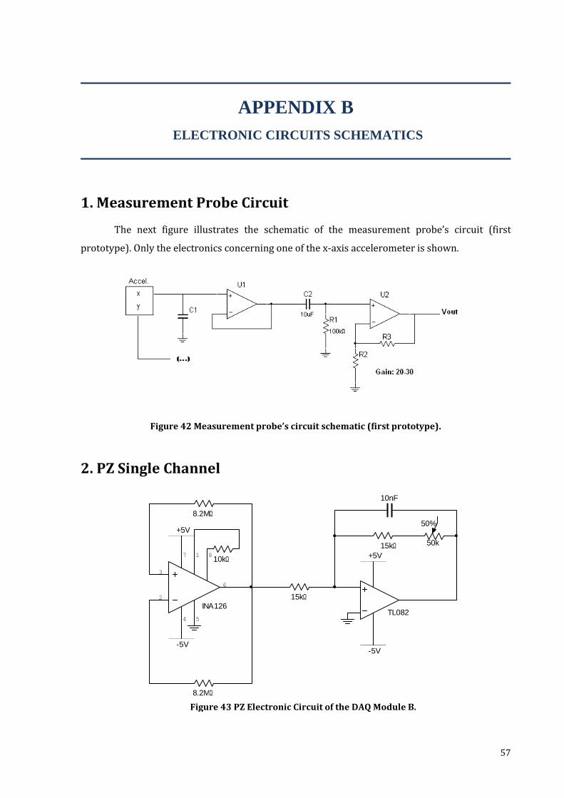
57
8.2MΩ
8.2MΩ
+5V
-5V
TL082
15kΩ
15kΩ 50k
50%
+5V
-5V
10nF
INA126
3
2
4
7
6
81
5
10kΩ
APPENDIX B
ELECTRONIC CIRCUITS SCHEMATICS
1. Measurement Probe Circuit
The next figure illustrates the schematic of the measurement probe’s circuit (first
prototype). Only the electronics concerning one of the x-axis accelerometer is shown.
Figure 42 Measurement probe’s circuit schematic (first prototype).
2. PZ Single Channel
Figure 43 PZ Electronic Circuit of the DAQ Module B.
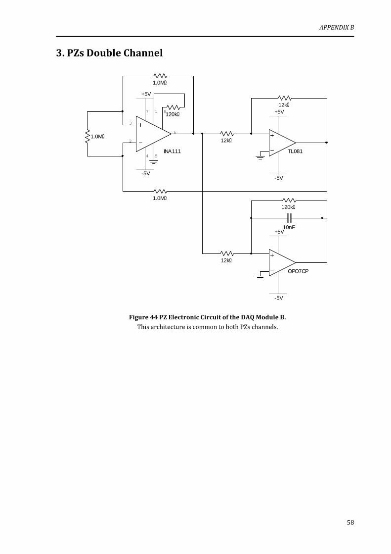
APPENDIX B
58
+5V
-5V
TL081
+5V
INA111
3
2
4
7
6
81
5
12kΩ
12kΩ
-5V
-5V
OPO7CP
+5V10nF
12kΩ
120kΩ
1.0MΩ
1.0MΩ
1.0MΩ
120kΩ
3. PZs Double Channel
Figure 44 PZ Electronic Circuit of the DAQ Module B.
This architecture is common to both PZs channels.
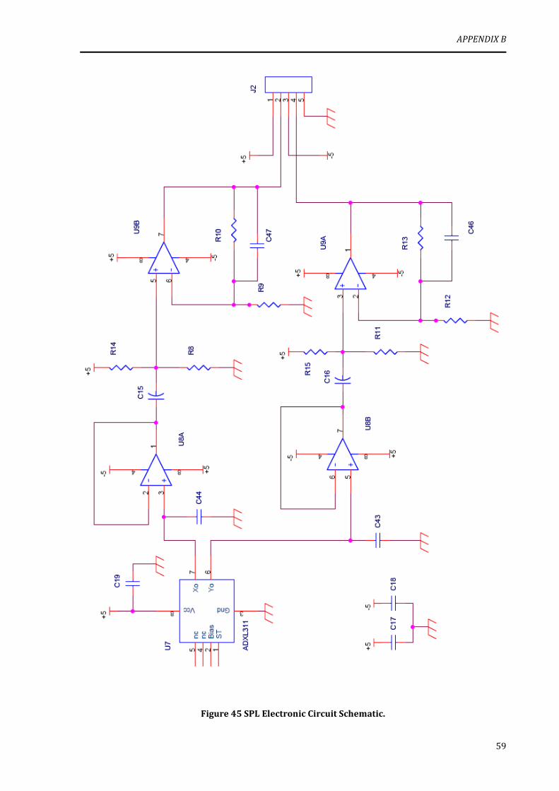
APPENDIX B
59
Figure 45 SPL Electronic Circuit Schematic.
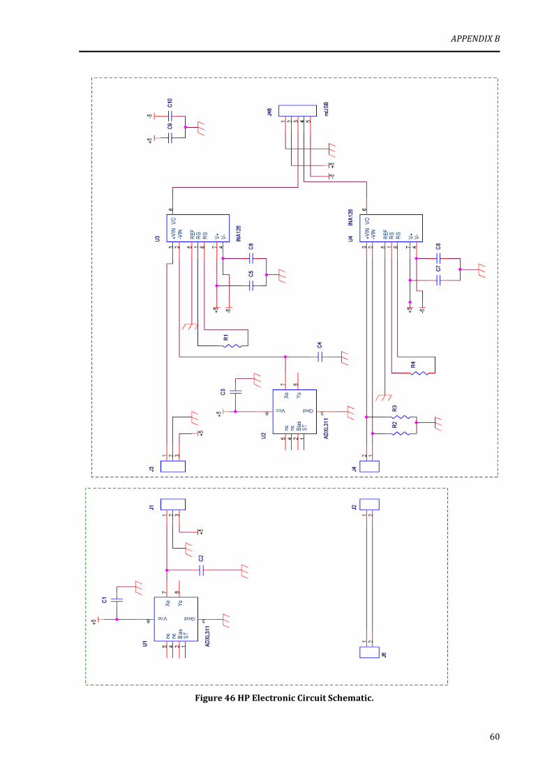
APPENDIX B
60
Figure 46 HP Electronic Circuit Schematic.
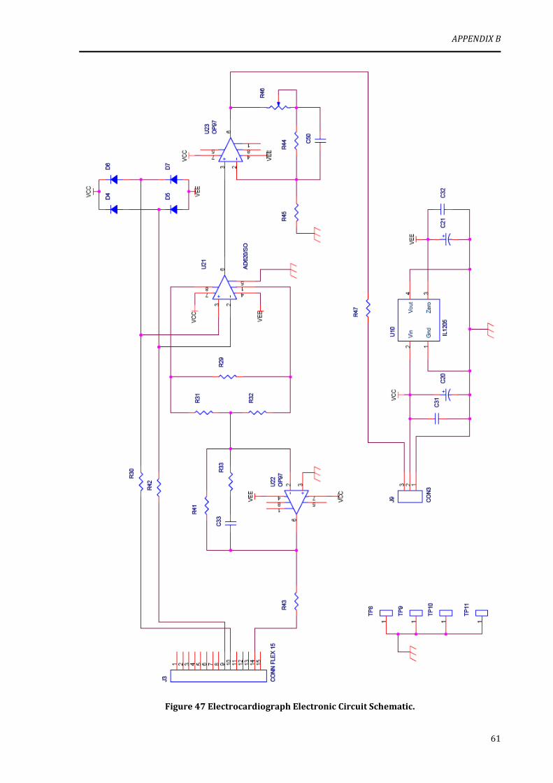
APPENDIX B
61
Figure 47 Electrocardiograph Electronic Circuit Schematic.