Relay Backpropagation for Effective Learning ofDeep Convolutional Neural Networks

Li Shen1, Zhouchen Lin2, Qingming Huang1

1 University of Chinese Academy of Sciences2 Key Lab. of Machine Perception (MOE), School of EECS, Peking University

Abstract. Learning deeper convolutional neural networks becomes atendency in recent years. However, many empirical evidences suggest thatperformance improvement cannot be gained by simply stacking more lay-ers. In this paper, we consider the issue from an information theoreticalperspective, and propose a novel method Relay Backpropagation, thatencourages the propagation of effective information through the networkin training stage. By virtue of the method, we achieved the first place inILSVRC 2015 Scene Classification Challenge. Extensive experiments ontwo challenging large scale datasets demonstrate the effectiveness of ourmethod is not restricted to a specific dataset or network architecture.Our models will be available to the research community later.

Keywords: Relay Backpropagation, Convolutional Neural Networks,Large scale image classification.

1 Introduction

Convolutional neural networks (CNNs) are capable of inducing rich featuresfrom data, and have been successfully applied in a variety of computer visiontasks. Many breakthroughs obtained in recent years benefit from the advancesof convolutional neural networks [1,2,3,4], spurring the research of pursuing ahigh performing network. The importance of network depth is revealed in thesesuccesses. For example, compared with AlexNet [1], the utilization of VGGNet [5]brings about substantial gains of accuracy on 1000-class ImageNet 2012 datasetby virtue of deeper architectures.

Increasing the depth of network becomes a promising way to enhance per-formance. On the downside, such solution is accompanied by the growth of pa-rameter size and model complexity, that poses great challenges for optimization.The training of deeper networks typically encounters the risk of divergence orslower convergence, and prone to overfitting. Besides, many empirical evidences[5,6,7] (e.g., the results reported by [5] on ImageNet dataset shown in Table 1(Left)) suggest that the improvement on accuracy cannot be trivially gained bysimply adding more layers. It is in accordance with the results in our preliminaryexperiments on Places2 challenge dataset [8], that deeper networks even sufferfrom a decline on performance (in Table 1 (Right)).

arX

iv:1

512.

0583

0v2

[cs

.CV

] 3

Apr

201

6

2

ModelImageNet 2012

top-1 err. top-5 err.

VGGNet-13 28.2 9.6

VGGNet-16 26.6 8.6

VGGNet-19 26.9 8.7

ModelPlaces2 challenge

top-1 err. top-5 err.

VGGNet-19 48.5 17.1

VGGNet-22 48.7 17.2

VGGNet-25 48.9 17.4

Table 1. Error rates (%) on ImageNet 2012 classification and Places2 challenge valida-tion set. The training and testing procedures for all models are the same. VGGNet-22and VGGNet-25 are obtained by simply adding 3 and 6 layers on VGGNet-19, respec-tively.

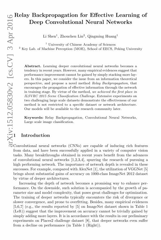
To interpret the phenomenon, we should be concerned with the possibilityof vanishing and exploding gradient which are the crucial reasons that hamperthe training of very deep networks with backpropagation [9] (BP) algorithm, asgradients might be prone to either very small or very large after backpropagationwith many layers. To investigate whether vanishing and exploding problems ap-pear, we analyze the scale of the gradients at different convolutional layers duringtraining. Take the 22-layer CNN model (in Table 1) as an example, shown inFig. 1. The average magnitude of gradients and their relative values with re-spect to weights are displayed, respectively. We can observe that the gradientmagnitude of lower layers does not tend to vanish or explode, but approxi-mately remain stable when performing the optimization. In practice, the issuesof vanishing and exploding gradient have been largely coped with by aid of sometechniques, e.g., rectifier neuron [10,11], refined initialization scheme [12,7], andBatch Normalization [13].

However, from an information theoretical perspective [14,15,16], the amountof information about target outputs diminishes during propagation, althoughthe gradient does not vanish. Such degradation will amplify as network goesdeeper. In order to effectively update network parameters, the error informationshould not go back too many layers. However, the problem is inevitable whenoptimizing a very deep network with standard backpropagation algorithm.

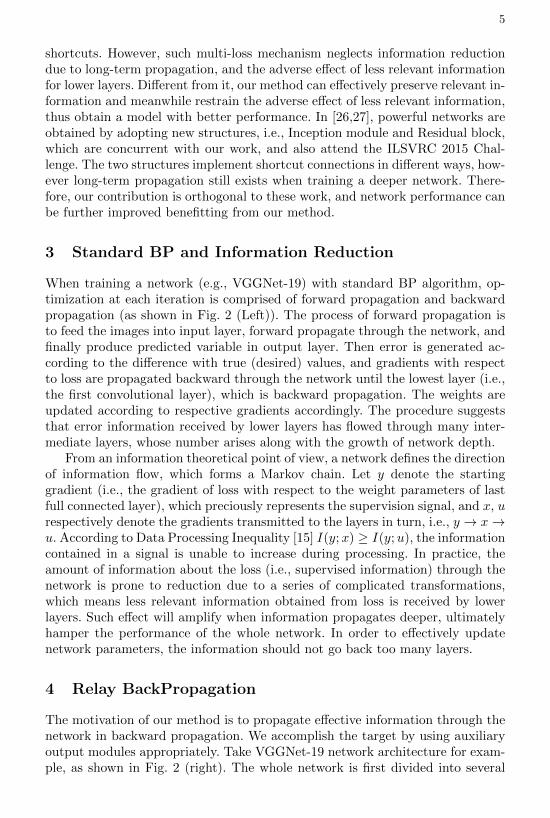
To address the problem, in this paper we propose a novel method, RelayBackpropagation (Relay BP), which encourages the propagation of effective in-formation through the network in training stage. To accomplish the aim, thewhole network is first divided into several segments. We introduce one or mul-tiple interim output modules (including loss layer) after intermediate segments,and aim to minimize the ensemble of losses. More importantly, the gradientsfrom different losses are propagated to the lowest layers of respective segments,namely, the gradient with respect to certain loss will propagate at most N con-secutive layers, where N is smaller than realistic network depth. An exampleframework is depicted in Fig. 2 with two auxiliary output modules. In a word,we provide an elegant way to effectively preserve relevant information by short-ening the path from outputs to lower layers, and meanwhile restrain the adverseeffect of less relevant information which propagated through too many layers.

3

1 4 7 10 13 16 190

0.002

0.004

0.006

0.008

0.01

layer index

mea

n ab

s. g

radi

ent

iter = 1e5iter = 2e5iter = 3e5

1 4 7 10 13 16 190.25

0.35

0.45

0.55

layer index

mea

n ab

s. g

radi

ent /

mea

n ab

s. w

eigh

t

iter = 1e5iter = 2e5iter = 3e5

Fig. 1. Magnitude of the gradient at each convolutional layer of the 22-layer CNNmodel (i.e., 19 convolutional layers and 3 fully connected layers) in Table 1. A colorline plot the gradient magnitude of different layers at a certain number of iterations.(Left) Average magnitude of gradients. (Right) Relative magnitude of gradients, i.e.,average magnitude of gradients divided by average magnitude of weights.

By virtue of Relay BP, we achieve the first place in ILSVRC 2015 SceneClassification Challenge, which provides a new large scale dataset involving 401classes and more than 8 million training images. The benefits of the method arealso verified on ImageNet 2012 classification dataset with another two famousnetwork architectures, which demonstrates our method is not constrained to aspecific architecture or dataset. We will make our models available to the researchcommunity.

2 Related Work

Convolutional neural networks have attracted much attention over the last fewyears. For image classification tasks with large scale data [17,18,19], there is atendency of increasing the network complexity (e.g., the depth [5] and the width[20]), which brings about the difficulties of training the network. A range oftechniques are exploited to address the problem by taking various angles. Forexample, Simonyan and Zisserman [5] propose to reduce the risk of divergenceby initializing a deeper network with the aid of pre-training shallower ones.Refined initialization schemes are adopted to train very deep networks directlyby drawing the weights from properly scaled distributions [12,7]. Moreover, thebenefits of new activation functions [10,7,21] for training deep networks havebeen shown in extensive experiments. Besides, some studies are developed inthe direction of finding better optimizers, such as stochastic gradient descentwith momentum [22] and RMSProp [23], which is widely used and works well inpractice.

It is particularly worthy of comparing our method with the work in [24,25],where temporary branches including classifiers are attached to intermediate lay-ers, and helps to propagate the supervision information to lower layers with

4

conv 3x3, 64

conv 3x3, 64

maxpool 2x2, 2

image

conv 3x3, 128

conv 3x3, 128

maxpool 2x2, 2

conv 3x3, 256

conv 3x3, 256

maxpool 2x2, 2

conv 3x3, 256

conv 3x3, 256

conv 3x3, 512

conv 3x3, 512

maxpool 2x2, 2

conv 3x3, 512

conv 3x3, 512

conv 3x3, 512

conv 3x3, 512

maxpool 2x2, 2

conv 3x3, 512

conv 3x3, 512

fc 4096

loss

fc 4096

fc 1000

conv 3x3, 64

conv 3x3, 64

maxpool 2x2, 2

image

conv 3x3, 128

conv 3x3, 128

maxpool 2x2, 2

conv 3x3, 256

conv 3x3, 256

maxpool 2x2, 2

conv 3x3, 256

conv 3x3, 256

conv 3x3, 512

conv 3x3, 512

maxpool 2x2, 2

conv 3x3, 512

conv 3x3, 512

conv 3x3, 512

conv 3x3, 512

maxpool 2x2, 2

conv 3x3, 512

conv 3x3, 512

fc 4096

loss

fc 4096

fc 1000

conv 3x3, 128

maxpool 4x4, 4

auxiliary loss1

fc 1024

fc 1024

conv 3x3, 128

maxpool 2x2, 2

auxiliary loss2

fc 1024

fc 1000

conv 3x3, 64

conv 3x3, 64

maxpool 2x2, 2

image

conv 3x3, 128

conv 3x3, 128

maxpool 2x2, 2

conv 3x3, 256

conv 3x3, 256

maxpool 2x2, 2

conv 3x3, 256

conv 3x3, 256

conv 3x3, 512

conv 3x3, 512

maxpool 2x2, 2

conv 3x3, 512

conv 3x3, 512

conv 3x3, 512

conv 3x3, 512

maxpool 2x2, 2

conv 3x3, 512

conv 3x3, 512

fc 4096

loss

fc 4096

fc 1000

conv 3x3, 128

maxpool 4x4, 4

auxiliary loss1

fc 1024

fc 1000

conv 3x3, 128

maxpool 2x2, 2

auxiliary loss2

fc 1024

fc 1000

Standard BP Relay BP

seg1

seg3

seg2

seg4

seg5

Fig. 2. (Left) VGGNet-19 network [5] with standard backpropagation algorithm. (Mid-dle & Right) VGGNet-19 extended network with Relay backpropagation algorithm.This is an example with two auxiliary output modules, adding two branches on tra-ditional VGGNet-19 architecture. The black arrows denote the forward propagationof information through the network, and the color arrows indicate the information(gradient) flows at backward propagation. This figure is best viewed on the screen.

5

shortcuts. However, such multi-loss mechanism neglects information reductiondue to long-term propagation, and the adverse effect of less relevant informationfor lower layers. Different from it, our method can effectively preserve relevant in-formation and meanwhile restrain the adverse effect of less relevant information,thus obtain a model with better performance. In [26,27], powerful networks areobtained by adopting new structures, i.e., Inception module and Residual block,which are concurrent with our work, and also attend the ILSVRC 2015 Chal-lenge. The two structures implement shortcut connections in different ways, how-ever long-term propagation still exists when training a deeper network. There-fore, our contribution is orthogonal to these work, and network performance canbe further improved benefitting from our method.

3 Standard BP and Information Reduction

When training a network (e.g., VGGNet-19) with standard BP algorithm, op-timization at each iteration is comprised of forward propagation and backwardpropagation (as shown in Fig. 2 (Left)). The process of forward propagation isto feed the images into input layer, forward propagate through the network, andfinally produce predicted variable in output layer. Then error is generated ac-cording to the difference with true (desired) values, and gradients with respectto loss are propagated backward through the network until the lowest layer (i.e.,the first convolutional layer), which is backward propagation. The weights areupdated according to respective gradients accordingly. The procedure suggeststhat error information received by lower layers has flowed through many inter-mediate layers, whose number arises along with the growth of network depth.

From an information theoretical point of view, a network defines the directionof information flow, which forms a Markov chain. Let y denote the startinggradient (i.e., the gradient of loss with respect to the weight parameters of lastfull connected layer), which preciously represents the supervision signal, and x, urespectively denote the gradients transmitted to the layers in turn, i.e., y → x→u. According to Data Processing Inequality [15] I(y;x) ≥ I(y;u), the informationcontained in a signal is unable to increase during processing. In practice, theamount of information about the loss (i.e., supervised information) through thenetwork is prone to reduction due to a series of complicated transformations,which means less relevant information obtained from loss is received by lowerlayers. Such effect will amplify when information propagates deeper, ultimatelyhamper the performance of the whole network. In order to effectively updatenetwork parameters, the information should not go back too many layers.

4 Relay BackPropagation

The motivation of our method is to propagate effective information through thenetwork in backward propagation. We accomplish the target by using auxiliaryoutput modules appropriately. Take VGGNet-19 network architecture for exam-ple, as shown in Fig. 2 (right). The whole network is first divided into several

6

segments separated with max-pooling layers. For example, from the first convo-lutional layer to the first max-pooling layer is considered as a segment, and thenext segment starts from the third convolutional layer and ends to the secondmax-pooling layer. Thus, there are totally five segments, numbered 1 to 5 fromlower to higher layers.

We attach one or multiple auxiliary output modules to intermediate seg-ments. Fig. 2 is an example with two output modules (i.e., auxiliary loss 1 andloss 2), which are added after segment 3 and 4, respectively. In order to preservethe relevant information about loss, the propagation of each loss is through atmost N consecutive layers, where N is the upper limit of the numbers of lay-ers that we deem that can carry enough relevant information. Namely, differentlosses are responsible for different parts of weight layers in the network. Theinformation flows from different losses are represented with different colors inFig. 2. Auxiliary loss 1 (colored with red) would be propagated until the lowestone in segment 1, and auxiliary loss 2 (colored with green) would be propagateduntil the lowest one in segment 3, and the primary loss (colored with blue) wouldbe propagated until the lowest layer in segment 4, respectively.

More importantly, there is overlapping between information flows at inter-mediate segments, such as segment 4 receives the information from primary lossand auxiliary loss 2. As our optimization objective is to minimize the sum ofthe three losses, the updating on segment 4 would fuse the information passedthrough from the two losses. Consequently, segment 4 plays the role of the tran-sition between the two information flows of primary loss and auxiliary loss 2, notonly the transition between lower and higher layers trivially, that is why we callthe method as Relay Backpropagation. Such mechanism is capable of alleviatingthe optimization difficulty at lower layers and favoring better discrimination athigher layers, and achieving the aim of coordinating the information propagationin a very deep network ultimately.

In summary, there are two distinct characters in our method: (1) differentlosses are responsible for different parts of weight layers in the network, ratherthan the all layers below. This is different from traditional multi-loss with stan-dard BP algorithm [24,25]. Such mechanism is helpful to reduce the degradationof relevant information about loss and restrain the adverse effect of less relevantinformation due to long-term propagation. (2) information flows from differentlosses exist overlapping at intermediate segments, that guarantees coordinateinformation propagation in the network.

In forward propagation step, information transmission follows the mannerfrom input to output layers, where the activations generated at one layer arefed into its adjacent layer in turn. The black arrows in Fig. 2 (middle) indicatethe directions of information flows through the network. It is consistent withstandard BP for the network with auxiliary branches.

When testing an image, a prediction is made without considering auxiliarybranches, as auxiliary supervision is introduced only to enhance the training ofnetwork. Consequently, there is no extra cost (parameter size and time expense)brought in testing stage, ensuring the test efficiency of model.

7

One might be concerned with: Where to add auxiliary output module? Andwhich segments (or convolutional layers) should belong to the scope of certainloss? We apply the heuristic scheme based on empirical evidences in this work.Nevertheless, some intuitive rules can be considered for guidance. One insightis that it is inadvisable to add auxiliary output modules at too lower layers,since the patterns captured at these layers lack of sufficient discrimination forrecognizing a high-level concept (e.g., object or scene). Moreover, the depth ofa network is an important factor to be considered. Adding an auxiliary branchmight be enough if the network is not too deep. In general, the design can beadjusted flexibly according to specific requirements and practical experience.

5 Experiments

In this section, we evaluate Relay BP on Places2 challenge [8] and ImageNet 2012classification dataset [19], and also investigate it on four different network ar-chitectures. We show Relay BP outperforms baselines significantly. The baselinemethods are briefly introduced below:

– Standard BP: Given the network, information forward and backwardpropagation follow the rule of traditional backpropagation algorithm (e.g.,in Fig. 2(Left)).

– Multi-loss + standard BP: One auxiliary output module (branch) isattached to parts of intermediate layers.

For a fair comparison, the network architecture in training stage (i.e., the ar-chitecture with temporary branches) is identical for our method and the baselineof multi-loss with standard BP. The difference lies in the scheme of informationbackward propagation. In the experiments, we only add one auxiliary branchfor all networks, as they are not too deep to tackle. Moreover, the incrementof branch also brings about training computation cost. Therefore, the principleis adding the branches as few as possible. We intend to train extremely deepernetworks by aid of multiple branches in future work.

5.1 Places2 Challenge

We evaluate our method on the Places2 challenge dataset [8], which is usedin ILSVRC 2015 Scene Classification Challenge. This dataset includes imagesbelonging to 401 scene categories, with 8.1M images for training, 20K imagesfor validation and 381K images for testing. To mimic the real-world frequenciesof scene occurrence, there is a non-uniform distribution of images per categoryfor training, ranging from 4,000 to 30,000. The classification performance ofthe challenge is evaluated using the top-5 error, which allows an algorithm toidentify multiple scene categories for an image, because many environments canbe described using different words.

8

input size gradient model A model B

224×224 2© [ conv 3×3, 64 ] × 2 [ conv 7×7, 128, stride 2 ] × 1

maxpool 2×2, 2

112×112 2© [ conv 3×3, 128 ] × 2

maxpool 2×2, 2 maxpool 2×2, 2

56×56 2© [ conv 3×3, 256 ] × 5 [ modified inception, k 64 ] × 4

maxpool 2×2, 2 maxpool 2×2, 2

28×28 1© 2© [ conv 3×3, 512 ] × 5 [ modified inception, k 128 ] × 4

maxpool 2×2, 2 maxpool 2×2, 2

- - auxiliary classifier 2©

14×14 1© [ conv 3×3, 256 ] × 5 [ modified inception, k 128 ] × 4

spp, {7, 3, 2, 1} spp, {7, 3, 2, 1}- 1© fc 4096

- 1© fc 4096

- 1© fc 401, classifier 1©

Table 2. Architectures of the networks used for ILSVRC 2015 Scene Classification.

The convolutional layer is denoted as “conv <receptive field>, <filters>”. The max-

pooling layer is denoted as “maxpool <region size>, <stride>”. Our modified inception

module concatenates the outputs of a 1×1 convolution with k filters, a 3×3 convolution

with k filters and two 3×3 convolution with 2k filters. 1© and 2© indicate which layersthe gradients propagate to.

Network Architectures. Relay BP is independent on the network architec-tures used. We investigate two types of deep convolutional neural network ar-chitectures on the Places2 challenge dataset, as shown in Table 2. The model Ais based on VGGNet-19 [5], and simply adds 3 convolutional layers on the threesmaller feature maps (56, 28, 14). The model B uses a 7× 7 convolutional layersand a modified inception module as building block. We also incorporate spatialpyramid pooling (spp) [28] into the models, where the pyramid configuration is7× 7, 3× 3, 2× 2 and 1× 1. Dropout regularization is applied to the first twofully-connected (fc) layers, with the dropout ratio 0.5. We use Rectified LinearUnit (ReLU) as nonlinearity and do not use Batch Normalization [13] in thetwo networks. The experiments involving Batch Normalization will be seen inSection 5.2. The auxiliary classifier 2© is used in multi-loss standard BP andRelay BP, rather than standard BP. The loss weight of the auxiliary classifier isset to 0.3. The “gradient” in Table 2 shows the details of backward propagationin Relay BP.

Class-aware Sampling. The Places2 challenge dataset has more than 8Mtraining images in total. The numbers of images in different classes are imbal-anced, ranging from 4,000 to 30,000 per class. The large scale data and non-uniform class distribution pose great challenges for model learning.

9

Methodmodel A model B

top-1 err. top-5 err. top-1 err. top-5 err.

standard BP 50.91 19.00 50.62 18.69

multi-loss + standard BP 50.72(0.19) 18.84(0.18) 50.59(0.03) 18.68(0.01)

Relay BP 49.75(1.16) 17.83(1.17) 49.77(0.85) 17.86(0.83)

Table 3. Single crop error rates (%) on Places2 challenge validation set. In thebrackets are the improvements over “standard BP” baseline.

Methodmodel A model B

top-1 err. top-5 err. top-1 err. top-5 err.

standard BP 48.67 17.19 48.29 16.89

multi-loss + standard BP 48.55(0.12) 17.05(0.14) 48.27(0.02) 16.89(0.00)

Relay BP 47.86(0.81) 16.33(0.86) 47.72(0.57) 16.36(0.53)

Table 4. Single model error rates (%) on Places2 challenge validation set. In thebrackets are the improvements over “standard BP” baseline.

To address this issue, we apply a sampling strategy, named “class-awaresampling”, during training. We aim to fill a mini-batch as uniform as possiblewith respect to classes, and prevent the same example and class from alwaysappearing in a permanent order. In practice, we use two types of lists, one isclass list, and the other is per-class image list. Taking Places2 challenge datasetfor example, we have one class list, and 401 per-class image lists. When getting atraining mini-batch in an iteration, we first sample a class X in the class list, thensample an image in the per-class image list of class X. When reaching the endof the per-class image list of class X, a shuffle operation is performed to reorderthe images of class X. When reaching the end of class list, a shuffle operationis performed to reorder the classes. We leverage such a class-aware samplingstrategy to effectively tackle the non-uniform class distribution, and the gain ofaccuracy on the validation set is about 0.6%.

Training and Testing. Our implementation is based on the publicly availablecode of Caffe [29]. We train models on the provided Places2 challenge trainingset, do not use any additional training data. The image is resized isotropicallyso that its shorter side is 256. To augment the training set, a 224×224 crop israndomly sampled from a training image, with the per-pixel mean subtracted.The random horizontal flipping and standard color shift in [1] are used. Weinitialize the weights using [7] and train all networks from scratch. We train thenetworks by applying stochastic gradient descent (SGD) with mini-batch size of256 and a fixed momentum of 0.9. The learning rate is initialized to 0.01, and isannealed by a factor of 10 when the error plateaus. The training is regularizedby weight decay (set to 0.0002). We train all models up to 80 × 104 iterations.In testing, we take the standard “single crop (center crop)” protocol in [25].

10

Team name top-5 err.

Ntu rose 19.33

Trimps-Soushen 17.98

Qualcomm Research 17.59

SIAT MMLAB 17.36

WM (model A) 17.35

WM (model B) 17.28

WM (model ensemble) 16.87

Table 5. The competition results of ILSVRC 2015 Scene Classification. The top-5error rates (%) is on Places2 challenge test set and reported by the test server. Oursubmissions are denoted as “WM”.

Furthermore, we use the fully-convolutional testing [5] to report the performanceof single model. The image is resized isotropically so that its shorter side is in{224, 256, 320, 384, 448}, and the scores are averaged at multiple scales.

Comparisons of Results. Table 3 lists the results of the three methods with“single crop” testing strategy. Compared with standard BP, the baseline “Multi-loss + standard BP” shows better performance by introducing auxiliary supervi-sion on intermediate layers, however the superiority is marginal, even negligiblewith regard to model B. In contrast, our method achieves significant improve-ment over standard BP, as well as consistently outperforms “Multi-loss + stan-dard BP” (approximately 1.0% on model A and 0.8% on model B based ontop-5 measure). It is notable that the improvement on model B is less thanthe one on model A. The shortcut connections in modified Inception modulesmake it possible to propagate information with shortcuts, somewhat alleviatesthe information reduction. This is also the reason of ineffectiveness of “Multi-loss+ standard BP” on model B. Nevertheless, our method is capable of improvingthe performance on model B. It confirms our insight that restraining the adverseeffect of less relevant information is helpful for training deep neural networks.

For a comprehensive comparison, we also report the model performance with“single model” testing strategy in Table 4. Clear advantage can be observedin our method compared to the baselines. It is worthy of mentioning that theimprovement of single model over center crop is less, about 1.5% top-5 errordiminished from 17.83% (single crop) to 16.33%, while empirical results on Ima-geNet 2012 classification dataset suggest the performance gain is approximately3.0% [7,13].

ILSVRC 2015 Scene Classification Challenge. By virtue of Relay BP, our“WM” team won the 1st place in ILSVRC 2015 Scene Classification task. Table5 shows the results of this challenge. Our five entries won the top five places, andthe results of our single model A and B outperform all ensemble results fromother teams. We combine five models of different architectures and input scales,

11

GT: art studio 1. art studio 2. art gallery 3. artists loft 4. art school 5. museum

GT: oilrig 1. oilrig 2. islet 3. ocean 4. coast 5. beach

GT: amusement park 1. amusement park 2. carrousel 3. amusement arcade 4. water park 5. temple

GT: sushi bar 1. sushi bar 2. restaurant kitchen 3. delicatessen 4. bakery shop 5. pantry

Fig. 3. Example images successfully classified by our method on Places2 challengevalidation set. For each image, the ground-truth label and our top-5 predictions arelisted.

GT: pub indoor 1. hotel room 2. bedroom 3. bedchamber 4. television room 5. balcony interior

GT: skyscraper 1. lift bridge 2. tower 3. bridge 4. viaduct 5. river

GT: waterfall block 1. aqueduct 2. viaduct 3. bridge 4. arch 5. hot spring

GT: entrance hall 1. corridor 2. hallway 3. elevator lobby 4. lobby 5. reception

Fig. 4. Example images incorrectly classified by our method on Places2 challenge vali-dation set. For each image, the ground-truth label and our top-5 predictions are listed.

and achieve 15.74% top-5 error on validation set. Our top-5 error is 16.87%on the testing set, which is roughly 1.1% worse than the validation result. Weconjecture that there might be a distribution gap between validation and testingdata, because similar degradation has also been observed by other teams [8]. Theimprovement of model ensemble over single model B is 0.4%. From single cropto single model, and further to model ensemble, the improvement is consistentlylower than expected. We conjecture that training with large scale data enhancesthe capability of single view, leading to the difficulties of further improvementwith model ensemble.

Fig. 3 shows some example images of Places2 challenge validation set, whichare successfully classified by our method. The predicted labels are in descendingorder of confidence. Even though many high-level scene concepts exist large intra-class appearance variance, our method can still recognize them easily. On theother hand, we also show some incorrectly classified examples in Fig. 4. Thesepredictions seem to be reasonable, although they fail in context of evaluationmeasure. A scene image might be typically described by multi-labels. Moreover,the composing of a scene is mostly complicated, such as a place is comprised ofmultiple objects and the same object might appear in different places. The loose

12

Method datasetResNet-50 Inception-v3

top-1 err. top-5 err. top-1 err. top-5 err.

standard BP [27,26] val 20.74 5.25 18.77 4.20

standard BP (re-implement)val

21.17 5.37 19.18 4.43

Relay BP 20.26 4.93 18.52 3.97

Relay BP test - 4.95 - 4.03

Table 6. Single model error rates (%) on ImageNet 2012 classification dataset.

connections between scene and object concepts increase the difficulties of scenerecognition.

5.2 ImageNet 2012 Classification

We evaluate our method on the ImageNet 2012 classification dataset [19], whichhas become one of the benchmarks to assess the progress of image classification.This dataset includes images belonging to 1000 classes, with 1.2M images fortraining, 50K images for validation and 100K images for testing. The classifi-cation performance is measured by the top-1 and top-5 error rates. We use theprovided data for training models, do not use any additional data.

Configurations. Recently, residual networks [27] introduce shortcut connec-tions, and has achieved state-of-the-art performance on ImageNet 2012 classi-fication dataset. Moreover, [26] utilizes the ”Inception-v3” architectures, andyielded comparable classification accuracy. We use the 50-layer residual network(ResNet-50) [27] and the Inception-v3 architectures [26] to evaluate Relay BP.For both architectures, we do not use scale jitter augmentation [5] during train-ing. Standard SGD is applied to train the networks. Other configurations (in-cluding data augmentation, network architectures, and training/testing method-ology) remain unchanged as [27,26]. More details about the configurations canbe found in [27,26]. For Relay BP, we add one auxiliary branch with the lossweight set to 0.3. The gradient overlapping segments of primary and auxiliaryloss range from “conv4 1” to “conv4 4” (ResNet-50), and “inception4a” to “in-ception4d” (Inception-v3), respectively. As the scheme of multi-loss has beenincluded in Inception-v3, we omit the baseline “Multi-loss + standard BP” inTable 6.

Results Analysis and Discussion. Table 6 lists the classification errorsachieved in single model. The results in the first row are the ones reportedin [27] and [26], respectively. And the second row displays the results by our re-implementation. There is slight difference between the two rows, mainly becauseof the diversity of details in implementation, which has been described in thesection of ”Configurations”.

13

The models trained with Relay BP achieve better classification performancecompared to the ones trained with standard BP. The accuracy improvementis 0.44% on top-5 measure, and 0.91% on top-1 measure based on ResNet-50network. Besides, there are 0.46% and 0.66% improvement on top-5 and top-1measure based on Inception-v3 architecture. The common characteristic of thetwo architectures is the utilization of shortcut connections, although the im-plementations are different. As we have mentioned in above sections, shortcutsmake the gradient of final outputs easily reach lower layers, thus are able toprevent the information reduction due to long-term propagation. This is alsothe evidence of only adding one auxiliary branch in Relay BP. Nevertheless,the network performance can be enhanced by aid of our method, which furtherdemonstrates the promise of our insight that restraining the adverse effect ofless relevance information is effective for improving network performance. Be-cause of the high baselines, the improvement is so difficult, which highlights theeffectiveness of our method. Moreover, we also report the results on test dataset(submitted to test server) to verify that the obtained results are not overfittingto the dataset. We only submitted the two results in the last half year, and theresult 4.03% outperforms the best result of single model reported in ILSVRC2015 ImageNet Classification task.

6 Conclusion

In this paper, we proposed the method Relay Backpropagation, which encour-ages the transmission of effective information in backward propagation of train-ing deep convolutional neural networks. Relevant information can be effectivelypreserved, and the adverse effect of less relevant information can be restrained.The experiments with four different network architectures on two challenginglarge scale datasets demonstrate the effectiveness of our method is not restrictedto certain network architecture or specific dataset. As a future direction, we areinterested in theoretical and mathematical support for the method.

References

1. Krizhevsky, A., Sutskever, I., Hinton, G.E.: ImageNet classification with deepconvolutional neural networks. In: NIPS. (2012)

2. Girshick, R., Donahue, J., Darrell, T., Malik, J.: Rich feature hierarchies for accu-rate object detection and semantic segmentation. In: CVPR. (2014)

3. Taigman, Y., Yang, M., Ranzato, M., Wolf, L.: Deepface: Closing the gap tohuman-level performance in face verification. In: CVPR. (2014)

4. Karpathy, A., Toderici, G., Shetty, S., Leung, T., Sukthankar, R., Fei-Fei, L.: Large-scale video classification with convolutional neural networks. In: CVPR. (2014)

5. Simonyan, K., Zisserman, A.: Very deep convolutional networks for large-scaleimage recognition. In: ICLR. (2015)

6. Srivastava, R.K., Greff, K., Schmidhuber, J.: Highway networks. In: ICML DeepLearning Workshop. (2015)

14

7. He, K., Zhang, X., Ren, S., Sun, J.: Delving deep into rectifiers: Surpassing human-level performance on imagenet classification. In: ICCV. (2015)

8. Zhou, B., Khosla, A., Lapedriza, A., Torralba, A., Oliva, A.: Places2: A large-scaledatabase for scene understanding. http://places2.csail.mit.edu/ (2015)

9. LeCun, Y., Bottou, L., Orr, G., Muller, K.: Efficient backprop. Neural Networks:Tricks of the trade (1998)

10. Nair, V., Hinton, G.: Rectified linear units improve restricted boltzmann machines.In: ICML. (2010)

11. Maas, A.L., Hannun, A.Y., Ng, A.Y.: Rectified nonlinearities improve neural net-work acstic models. In: ICML. (2013)

12. Glorot, X., Bengio, Y.: Understanding the difficulty of training deep feedforwardneural networks. In: ICAIS. (2010)

13. Ioffe, S., Szegedy, C.: Batch normalization: Accelerating deep network training byreducing internal covariate shift. arXiv:1502.03167 (2015)

14. Kamimura, R.: Information Theoretic Neural Computation. World Scientific(2002)

15. Cover, T.M., Thomas, J.A.: Elements of Information Theory. Wiley-Interscience(2006)

16. Tishby, N., Zaslavsky, N.: Deep learning and the information bottleneck principle.In: IEEE Information Theory Workshop. (2015)

17. Zhou, B., Lapedriza, A., Xiao, J., Torralba, A., Oliva, A.: Learning deep featuresfor scene recognition using places database. In: NIPS. (2014)

18. Xiao, J., Ehinger, K., Hays, J., Torralba, A., Oliva, A.: Sun database: Exploringa large collection of scene categories. IJCV (2014)

19. Russakovsky, O., Deng, J., Su, H., Krause, J., Satheesh, S., Ma, S., Huang, Z.,Karpathy, A., Khosla, A., Bernstein, M., Berg, A.C., Fei-Fei, L.: Imagenet largescale visual recognition challenge. IJCV (2015)

20. Zeiler, M.D., Fergus, R.: Visualizing and understanding convolutional neural net-works. In: ECCV. (2014)

21. Goodfellow, I.J., Warde-Farley, D., Mirza, M., Courville, A., Bengio, Y.: Maxoutnetworks. arXiv:1302.4389 (2013)

22. Sutskever, I., Martens, J., Dahl, G.E., Hinton, G.E.: On the importance of initial-ization and momentum in deep learning. In: ICML. (2013)

23. Tieleman, T., Hinton, G.: Divide the gradient by a running average of its recentmagnitude. COURSERA: Neural Networks for Machine Learning (2012)

24. Lee, C.Y., Xie, S., Gallagher, P., Zhang, Z., Tu, Z.: Deeply-supervised nets. In:AISTATS. (2015)

25. Szegedy, C., Liu, W., Jia, Y., Sermanet, P., Reed, S., Anguelov, D., Erhan, D.,Vanhoucke, V., Rabinovich, A.: Going deeper with convolutions. In: CVPR. (2015)

26. Szegedy, C., Vanhoucke, V., Ioffe, S., Shlens, J., Wojna, Z.: Rethinking the incep-tion architecture for computer vision. arXiv:1512.00567 (2015)

27. He, K., Zhang, X., Ren, S., Sun, J.: Deep residual learning for image recognition.In: CVPR. (2016)

28. He, K., Zhang, X., Ren, S., Sun, J.: Spatial pyramid pooling in deep convolutionalnetworks for visual recognition. In: ECCV. (2014)

29. Jia, Y., Shelhamer, E., Donahue, J., Karayev, S., Long, J., Girshick, R., Guadar-rama, S., Darrell, T.: Caffe: Convolutional architecture for fast feature embedding.arXiv:1408.5093 (2014)