reliability based safety level evaluation …etd.lib.metu.edu.tr/upload/12612723/index.pdfcontinuous...
TRANSCRIPT
RELIABILITY BASED SAFETY LEVEL EVALUATION OF TURKISH TYPE PRECAST PRESTRESSED CONCRETE BRIDGE GIRDERS
DESIGNED IN ACCORDANCE WITH THE LOAD AND RESISTANCE FACTOR DESIGN METHOD
A THESIS SUBMITTED TO THE GRADUATE SCHOOL OF NATURAL AND APPLIED SCIENCES
OF MIDDLE EAST TECHNICAL UNIVERSITY
BY OKTAY ARGINHAN
IN PARTIAL FULFILLMENT OF THE REQUIREMENTS FOR
THE DEGREE OF MASTER OF SCIENCE IN
CIVIL ENGINEERING
DECEMBER 2010

Approval of the thesis:
RELIABILITY BASED SAFETY LEVEL EVALUATION OF TURKISH TYPE PRECAST PRESTRESSED CONCRETE BRIDGE GIRDERS
DESIGNED IN ACCORDANCE WITH THE LOAD AND RESISTANCE FACTOR DESING METHOD
submitted by OKTAY ARGINHAN in partial fulfillment of the requirements for the degree of Master of Science in Civil Engineering Department, Middle East Technical University by,
Prof. Dr Canan Özgen Dean, Graduate School of Natural and Applied Sciences
Prof. Dr. Güney Özcebe
Head of Department, Civil Engineering Assist. Prof. Dr. Alp Caner Supervisor, Civil Engineering Dept., METU Prof. Dr. M. Semih Yücemen Co-Supervisor, Civil Engineering Dept., METU Examining Committee Members: Assist. Prof. Dr Ayşegül Askan Gündoğan Civil Engineering Dept., METU Assist. Prof. Dr. Alp Caner Civil Engineering Dept., METU Prof. Dr. M. Semih Yücemen
Civil Engineering Dept., METU Assist. Prof. Dr Afşin Sarıtaş Civil Engineering Dept., METU Yeşim Esat General Directorate of Highways of Turkey Date:

iii
I hereby declare that all information in this document has been obtained and presented in accordance with academic rules and ethical conduct. I also declare that, as required by these rules and conduct, I have fully cited and referenced all material and results that are not original to this work.
Name, Last name: Oktay Argınhan Signature :

iv
ABSTRACT
RELIABILITY BASED SAFETY LEVEL EVALUATION OF TURKISH
TYPE PRECAST PRESTRESSED CONCRETE BRIDGE GIRDERS
DESIGNED IN ACCORDANCE WITH THE LOAD AND RESISTANCE
FACTOR DESING METHOD
Argınhan, Oktay
M.S., Department of Civil Engineering
Supervisor: Assist. Prof. Dr. Alp Caner
Co-Supervisor: Prof. Dr. M. Semih Yücemen
December 2010, 137 pages
The main aim of the present study is to evaluate the safety level of Turkish
type precast prestressed concrete bridge girders designed according to
American Association of State Highway and Transportation Officials Load and
Resistance Factor Design (AASHTO LRFD) based on reliability theory. Span
lengths varying from 25 m to 40 m are considered. Two types of design truck
loading models are taken into account: H30S24-current design live load of
Turkey and HL93-design live load model of AASHTO LRFD. The statistical
parameters of both load and resistance components are estimated from local
data and published data in the literature. The bias factors and coefficient of
variation of live load are estimated by extrapolation of cumulative distribution
functions of maximum span moments of truck survey data (Axle Weight
Studies) that is gathered from the Division of Transportation and Cost Studies
of the General Directorate of Highways of Turkey. The uncertainties associated

v
with C40 class concrete and prestressing strands are evaluated by the test data
of local manufacturers. The girders are designed according to the requirements
of both Service III and Strength I limit states. The required number of strands
is calculated and compared.
Increasing research in the field of bridge evaluation based on structural
reliability justifies the consideration of reliability index as the primary measure
of safety of bridges. The reliability indexes are calculated by different methods
for both Strength I and Service III limit states. The reliability level of typical
girders of Turkey is compared with those of others countries. Different load
and resistance factors are intended to achieve the selected target reliability
levels. For the studied cases, a set of load factors corresponding to different
levels of reliability index is suggested for the two models of truck design loads.
Analysis with Turkish type truck models results in higher reliability index
compared to the USA type truck model for the investigated span lengths
Keywords: Reliability Analysis, Reliability Index, Bridge Live Load Models,
Prestressed Precast Bridge Girders, Target Reliability Level, Bridges of
Turkey.
vi
ÖZ
YÜK VE DAYANIM KATSAYILARI TASARIM YÖNTEMĐNE GÖRE
TASARLANMIŞ, TÜRKĐYE'DE KULLANILAN PREFABRĐK
ÖNGERMELĐ KÖPRÜ KĐRĐŞLERĐNĐN GÜVENĐRLĐK DÜZEYLERĐNĐN
DEĞERLENDĐRMESĐ
Argınhan, Oktay
Yüksek Lisans, Đnşaat Mühendisliği Bölümü
Tez Yöneticisi: Yrd. Doç. Dr. Alp Caner
Ortak Tez Yöneticisi: Prof. Dr. M. Semih Yücemen
Aralık 2010, 137 sayfa
Bu tez çalışmasında, AASHTO LRFD şartnamesine göre tasarlanmış,
Türkiye’de kullanılan öngermeli prefabrik köprü kirişlerinin güvenirlik
seviyesi değerlendirilmiştir. 25m’den 40m’ye kadar açıklığa sahip köprüler göz
önünde tutulmuştur. Yük ve dayanımın istatistiksel parametreleri, yerel
verilerden ve uluslararası çalışmalardan elde edilmiştir. Đki tip tasarım
kamyonu yük modeli hesaba katılmıştır; H30S24 - Türkiye’de tasarımda
kullanılan tasarım kamyon yüklemesi ve HL93-AASHTO LRFD de belirtilen
tasarım kamyonu yüklemesi. Karayolları Genel Müdürlüğü, Ulaşım ve Maliyet
Etütleri şubesinden alınan dingil ağırlığı etüt verileri ile hesaplanan orta açıklık
maksimum momentleri kullanılarak birikimli dağlım işlevi Gumbel olasılık
kâğıdına çizilmiştir ve bu dağlımlar daha uzun periyotlara extrapole edilerek
tasarım kamyon yükü istatistiksel parametreleri belirlenmiştir. Yerel
üreticilerden alınan test verileri kullanılarak C40 beton sınıfı ve öngerme

vii
halatının dayanımlarına ilişkin istatistiksel parametreler belirlenmiştir.
Öngerilmeli kirişler, servis ve mukavemet sınır durumları düşünülerek
tasarlanmış ve gerekli öngerilme halat sayıları belirlenerek her iki sınır durumu
için karşılaştırılmıştır.
Yapısal güvenirlik esasına dayalı köprü değerlendirme alanında yapılan
çalışmalar, güvenirlik indeksinin köprü yapı emniyetinin temel ölçüsü
olduğunu doğrulamaktadır. Bu çalışmada, farklı metodlar kullanılarak hem
servis hem de mukavemet sınır durumları için güvenirlik indeksi
hesaplanmıştır ve karşılaştırılmıştır. Türkiye’deki belirsizliklere göre
tasarlanan tipik öngerilmeli köprü kirişlerinin güvenirlik seviyesi diğer
ülkelerin belirsizlikleri ve tasarım şartnameleri ile karşılaştırılmıştır. Belirlenen
hedef güvenirlik seviyelerine göre farklı yük ve dayanım katsayıları elde
edilmiştir.
Anahtar Kelimeler: Güvenirlik Analizi, Güvenirlik Đndeksi, Köprü Hareketli
Yük Modelleri, Öngermeli Prefabrik Köprü Kirişleri, Hedef Güvenirlik
Seviyesi, Türkiye’deki Köprüler.

viii
To My Parents,

ix
ACKNOWLEDGMENTS
The author deeply appreciates his supervisor Assist. Prof. Dr. Alp Caner for the
continuous guidance and constructive criticism he has provided throughout the
preparation of the thesis. Without his encouragement and patience, this thesis
would not have been completed.
The author wishes to express his deepest gratitude to his co-supervisor Prof.
Dr. M. Semih Yücemen for sharing his valuable experience and knowledge,
making helpful suggestions, giving real insight into my focus throughout the
research.
The author also would like to thank Turkish General Directorate of Highways
for providing data and guidance in this study.
The author extends his gratefulness to PROYA Software and Engineering
(PROKON) and to his colleagues, who have provided him with great support,
while he was both studying and working.
Finally, the author wants to express his sincere thanks to his parents, Bahattin
and Zeynep Argınhan and his sister Çiğdem Argınhan and his brother Okan
Argınhan for the encouragement and love they have given him not only
throughout the completion of this thesis but also his whole life.

x
TABLE OF CONTENTS
ABSTRACT ...................................................................................................... iv
ÖZ...................................................................................................................... vi
ACKNOWLEDGMENTS................................................................................. ix
TABLE OF CONTENTS ................................................................................... x
LIST OF TABLES .......................................................................................... xiii
LIST OF FIGURES......................................................................................... xvi
LIST OF SYMBOLS....................................................................................... xxi
LIST OF SYMBOLS....................................................................................... xxi
CHAPTERS........................................................................................................ 1
1. INTRODUCTION.......................................................................................... 1
1.1 OBJECTIVES....................................................................................... 3
1.2 SCOPE.................................................................................................. 4
2. LITERATURE SURVEY / BACKGROUND ............................................... 6
2.1 REVIEW OF LITERATURE............................................................... 6
3. STATISTICS OF LOAD.............................................................................. 18
3.1 DESIGN LIMIT STATES AND LOAD COMBINATIONS ............ 18
3.2 DEAD LOAD..................................................................................... 21
3.3 LIVE LOAD....................................................................................... 22
3.3.1 Live Load Models ...................................................................... 22
3.3.2 Evaluation of Truck Survey Data ............................................... 28
3.3.3 Assessment of the Statistical Parameters of Live Load ............. 38

xi
3.4 DYNAMIC LOAD ALLOWANCE................................................... 68
3.5 GIRDER DISTRIBUTION FACTOR ............................................... 71
3.6 SUMMARY OF STATISTICAL PARAMETERS OF LOAD ......... 73
4. STATISTICS OF RESISTANCE ................................................................ 74
4.1 NOMINAL FLEXURAL RESISTANCE CAPACITY ACCORDING
TO AASHTO LRFD DESIGN SPECIFICATION ........................................ 74
4.2 TENSILE STRESS CHECK ACCORDING TO SERVICE III LIMIT
STATE............................................................................................................ 78
4.3 ASSESSMENT OF THE STATISTICAL PARAMETERS OF THE
RESISTANCE VARIABLES ........................................................................ 81
4.3.1 Concrete...................................................................................... 81
4.3.2 Prestressing Strand ..................................................................... 94
4.3.3 Dimensions................................................................................. 98
4.4 SUMMARY OF THE STATISTICAL PARAMETERS OF
RESISTANCE.............................................................................................. 100
5. TURKISH TYPE PRECAST PRESTRESSED CONCRETE BRIDGE
GIRDERS....................................................................................................... 101
5.1 TYPICAL CROSS-SECTIONS OF PRECAST PRESTRESSED
CONCRETE GIRDERS............................................................................... 101
5.2 TYPICAL BRIDGE CROSS-SECTIONS ....................................... 103
5.3 DESIGN OF BRIDGES ................................................................... 106
6. RELIABILITY-BASED SAFETY LEVEL EVALUATION.................... 111
6.1 LIMIT STATE FUNCTION ............................................................ 111
6.2 RELIABILITY LEVEL ACCORDING TO AASHTO LRFD BASED
ON LOCAL CONDITIONS ........................................................................ 115
6.3 COMPARISON WITH OTHER DESING CODES AND
COUNTRIES................................................................................................ 119
6.4 CODE CALIBRATION AND TARGET RELIABILITY LEVEL . 123
6.5 LOAD AND RESISTANCE FACTORS ......................................... 124

xii
7. CONCLUSION .......................................................................................... 130
7.1 CONCLUDING COMMENTS........................................................ 130
7.2 RECOMMENDATIONS FOR FUTURE STUDIES....................... 133
REFERENCES............................................................................................... 134

xiii
LIST OF TABLES
TABLES
Table 3-1 Statistical Parameters of Dead Load from Nowak et al. [12] .......... 22
Table 3-2 Maximum Span Moment due to HL-93........................................... 27
Table 3-3 Maximum Span Moment due to H30-S24 ....................................... 27
Table 3-4 Partial Sample Data for Axle Weight Measurements (BABAESKĐ-
LÜLEBURGAZ Direction) [24] ............................................................... 30
Table 3-5 Notation of Axle Types.................................................................... 31
Table 3-6 Vehicle Type.................................................................................... 31
Table 3-7 Assumed Truck Axle Distances....................................................... 34
Table 3-8 Number of Trucks vs. Time Period and Probability ........................ 49
Table 3-9 Mean Maximum Moment Ratios for H30-S24 (Overall) ................ 50
Table 3-10 Mean Maximum Moment Ratios for HL-93 (Overall).................. 50
Table 3-11 Mean Maximum Moment Ratios for H30-S24 (Upper Tail)......... 50
Table 3-12 Mean Maximum Moment Ratios for HL-93 (Upper Tail) ............ 51
Table 3-13 Mean Maximum Moment Ratios for H30-S24 (Extreme) ............. 51
Table 3-14 Mean Maximum Moment Ratios for HL-93 (Extreme)................. 51
Table 3-15 Mean, Standard Deviation and Coefficient of Variation Values
Computed from the Whole Data for each Span ........................................ 58
Table 3-16 Parameters of Gumbel Distribution (Overall) ............................... 60
Table 3-17 Mean, Standard Deviation and Coefficient of Variation of Moment
Ratios (Overall) Estimated According to Gumbel Distribution ............... 60
Table 3-18 Parameters of Gumbel Distribution (Upper Tail).......................... 61
Table 3-19 Mean, Standard Deviation and Coefficient of Variation of Moment
Ratios (Upper Tail) Estimated According to Gumbel Distribution.......... 61
Table 3-20 Parameters of Gumbel Distribution (Extreme) .............................. 61
xiv
Table 3-21 Mean, Standard Deviation and Coefficient of Variation of Moment
Ratios (Extreme) Estimated According to Gumbel Distribution .............. 62
Table 3-22 Maximum One Lane Truck Moment for H30S24 Loading ........... 67
Table 3-23 Maximum One Lane Truck Moment for HL93 Loading............... 67
Table 3-24 Dynamic Load Allowance, IM (AASHTO LRFD Table
3.6.2.1-1) ................................................................................................... 68
Table 3-25 Statistical Parameters of the Dynamic Load Factors (DLF) for
Prestressed Concrete Girder Bridges [16]................................................. 70
Table 3-26 Summary of Statistical Parameters of Load................................... 73
Table 4-1 Statistical Parameters of Compressive Strength Data According to
Years for Turkey [5] ................................................................................. 83
Table 4-2 Statistical Parameters of 28 day Compressive Strength Data
According to Concrete Class for Turkey [5]............................................. 84
Table 4-3 Statistical Parameters of 7 and 28 day Laboratory (Cylinder)
Compressive Strength Data of Firm 1 According to C40 Concrete Class 86
Table 4-4 Statistical Parameters of 7 and 28 day Laboratory (Cylinder)
Compressive Strength Data of Firm 2 According to C40 Concrete Class 86
Table 4-5 Statistical Parameters of 7 and 28 day Laboratory (Cylinder)
Compressive Strength Data of Firm 1 and Firm 2 for C40 Concrete
Class .......................................................................................................... 87
Table 4-6 Statistical Parameters of (Cylinder) Compressive Strength of C30
and C40 Concrete Class ............................................................................ 94
Table 4-7 Statistical Parameters of Laboratory Yield Strength of Strand........ 96
Table 4-8 Statistical Parameters of Prestressing Strand................................... 97
Table 4-9 Recommended Ranges and Values of the Statistical Parameters of
Beam Dimensions [7]................................................................................ 98
Table 4-10 Summary of Statistical Parameters of Resistance........................ 100
Table 5-1 Selected Precast Prestressed Concrete Girder Bridges .................. 103
Table 5-2 Calculated Moments due to Dead and Live Loads per Girder....... 106

xv
Table 5-3 Results of Design According to Strength I Limit State for
H30S24.................................................................................................... 107
Table 5-4 Results of Design According to Strength I and Service III Limit
States for H30S24 ................................................................................... 108
Table 5-5 Results of Design According to Strength I Limit State for HL93 . 108
Table 5-6 Results of Design According to Strength I and Service III Limit
States for HL93 ....................................................................................... 108
Table 6-1 Reliability Index and the Corresponding Failure Probability
Assuming Normal Distribution............................................................... 113
Table 6-2 Reliability Indexes Calculated by Alternative Reliability Methods for
Different Loading and Limit States Based on Local Conditions of
Turkey ..................................................................................................... 117
Table 6-3 Reliability Indexes Corresponding to Bridge Designs of Various
Countries and Design Codes ................................................................... 120
Table 6-4 Reliability Index Values Corresponding to Different Load and
Resistance Factor Combinations for H30S24 Loading........................... 126
Table 6-5 Reliability Index Values Corresponding to Different Load and
Resistance Factor Combinations for HL93 Loading............................... 127
Table 7-1 Summary of Statistical Parameters Assessed Using Turkish Data 132
xvi
LIST OF FIGURES
FIGURES
Figure 2-1 Extrapolated Moment Ratios Obtained from Truck Survey Data
[12] .............................................................................................................. 7
Figure 2-2 Bias Factor for Simple Span Moment: Ratio of M(75) / M(HL93)
and M(75) / M(HS20) [13].......................................................................... 8
Figure 2-3 Reliability Indexes for Prestressed Concrete Girders-Span
Moments; AASHTO (Standard 1992) [12]................................................. 9
Figure 2-4 Reliability Indexes for Prestressed Concrete Girders-Span
Moments; Proposed LRFD Code (Current AASHTO LRFD) [12] .......... 11
Figure 2-5 Monte Carlo Results for All Bridges [13] ...................................... 12
Figure 2-6 Beta Factors for Various Types of P/S Concrete Girders [13] ....... 12
Figure 2-7 Moment Ratios Obtained from Spanish Truck Survey [3]............. 14
Figure 2-8 Bias Factors for the Moment per Girder (including Dynamic load
Factor, DLF) for the Ontario Truck Data and Spanish Truck Data, with the
Nominal Moment Corresponding to AASHTO LRFD [3] ....................... 14
Figure 2-9 Reliability Indexes for Ontario Truck Traffic [3]........................... 15
Figure 2-10 Reliability Indexes for Spanish Truck Traffic [3] ........................ 15
Figure 2-11 Number of 12.7 mm Strands per Girder Required for Strength and
Service Limit States [17]........................................................................... 16
Figure 2-12 Reliability Indexes for Flexural Capacity Based on the
Requirements of the Strength Limit State in the Three Codes [17].......... 17
Figure 2-13 Reliability Indexes for Flexural Capacity Based on the
Requirements of the Service Limit State in the Three Codes [17] ........... 17
Figure 3-1 Characteristics of Design Truck, HL-93......................................... 23
Figure 3-2 Design Live Load in AASHTO LRFD,HL-93 ............................... 24
xvii
Figure 3-3 Characteristics of Design Truck, H30-S24..................................... 25
Figure 3-4 Design Live Load in Turkey, H30-S24 [14]................................... 26
Figure 3-5 Comparison of Maximum Span Moments due to HL93 and H30S24
Corresponding to Different Span Length.................................................. 27
Figure 3-6 Example of Axle Type Notation..................................................... 31
Figure 3-7 Histogram of Vehicles according to Axle Types............................ 32
Figure 3-8 Histogram of Gross Vehicle Weights (GVW) of Surveyed Trucks 33
Figure 3-9 Histogram of Surveyed Truck Span Moments for 25 m Span
Length ....................................................................................................... 35
Figure 3-10 Histogram of Surveyed Truck Span Moments for 30 m Span
Length ....................................................................................................... 35
Figure 3-11 Histogram of Surveyed Truck Span Moments for 35 m Span
Length ....................................................................................................... 36
Figure 3-12 Histogram of Surveyed Truck Span Moments for 40 m Span
Length ....................................................................................................... 36
Figure 3-13 Plot of Moment Ratios Computed Based on Overall Truck Survey
Data on Normal Probability Paper (H30S24) ........................................... 41
Figure 3-14 Plot of Moment Ratios Computed Based on Overall Truck Survey
Data on Normal Probability Paper (HL93) ............................................... 42
Figure 3-15 Straight Lines Fitted to Overall Moment Ratios on Normal (NP)
and Gumbel (GP) Probability Papers (H30S24-25 m span) ..................... 42
Figure 3-16 Straight Lines Fitted to Overall Moment Ratios on Normal (NP)
and Gumbel (GP) Probability Papers (HL93-25 m span) ......................... 43
Figure 3-17 Straight Lines Fitted to Overall Moment Ratios on Normal (NP)
and Gumbel (GP) Probability Papers (H30S24-30 m span) ..................... 43
Figure 3-18 Straight Lines Fitted to Overall Moment Ratios on Normal (NP)
and Gumbel (GP) Probability Papers (HL93-30 m span) ......................... 43
Figure 3-19 Straight Lines Fitted to Overall Moment Ratios on Normal (NP)
and Gumbel (GP) Probability Papers (H30S24-35 m span) ..................... 44

xviii
Figure 3-20 Straight Lines Fitted to Overall Moment Ratios on Normal (NP)
and Gumbel (GP) Probability Papers (HL93-35 m span) ......................... 44
Figure 3-21 Straight Lines Fitted to Overall Moment Ratios on Normal (NP)
and Gumbel (GP) Probability Papers (H30S24-40 m span) ..................... 44
Figure 3-22 Straight Lines Fitted to Overall Moment Ratios on Normal (NP)
and Gumbel (GP) Probability Papers (HL93-40 m span) ......................... 45
Figure 3-23 Straight Lines Fitted to the Upper Tail of Moment Ratios Plotted
on Gumbel (GP) Probability Papers (25 m span) ..................................... 45
Figure 3-24 Straight Lines Fitted to the Upper Tail of Moment Ratios Plotted
on Gumbel (GP) Probability Papers (30 m span) ..................................... 45
Figure 3-25 Straight Lines Fitted to the Upper Tail of Moment Ratios Plotted
on Gumbel (GP) Probability Papers (35 m span) ..................................... 46
Figure 3-26 Straight Lines Fitted to the Upper Tail of Moment Ratios Plotted
on Gumbel (GP) Probability Papers (40 m span) ..................................... 46
Figure 3-27 Straight Lines Fitted to Extreme Surveyed Truck Moments on
Gumbel (GP) Probability Papers (25 m span) .......................................... 46
Figure 3-28 Straight Lines Fitted to Extreme Surveyed Truck Moments on
Gumbel (GP) Probability Papers (30 m span) .......................................... 47
Figure 3-29 Straight Lines Fitted to Extreme Surveyed Truck Moments on
Gumbel (GP) Probability Papers (35 m span) .......................................... 47
Figure 3-30 Straight Lines Fitted to Extreme Surveyed Truck Moments on
Gumbel (GP) Probability Papers (40 m span) .......................................... 47
Figure 3-31 Extrapolated Moment Ratios for H30-S24 (Overall) .................. 52
Figure 3-32 Extrapolated Moment Ratios for HL93 (Overall) ....................... 53
Figure 3-33 Extrapolated Moment Ratios for H30-S24 (Upper Tail)............. 54
Figure 3-34 Extrapolated Moment Ratios for HL93 (Upper Tail).................. 55
Figure 3-35 Extrapolated Moment Ratios for H30-S24 (Extreme) ................. 56
Figure 3-36 Extrapolated Moment Ratios for HL93 (Extreme) ...................... 57

xix
Figure 3-37 Variation of 75 year Mean Maximum Moment Ratio with Span
Lengths According to Different Assumptions on Extrapolation of Data for
H30S24...................................................................................................... 63
Figure 3-38 Variation of 75 year Mean Maximum Moment Ratio with Span
Lengths According to Different Assumptions on Extrapolation of Data for
HL93 ......................................................................................................... 63
Figure 3-39 Comparison of the Coefficients of Variation Obtained from
Different Assumptions .............................................................................. 64
Figure 3-40 Sketch of Two Truck in Single Lane........................................... 66
Figure 3-41 Maximum Static and Dynamic Deflections [16]......................... 69
Figure 3-42 Dynamic Load Factors for One Truck and Two Trucks [16]...... 70
Figure 4-1 Forces on Reinforced Concrete Beam [4] ...................................... 75
Figure 4-2 Combined Histogram of 7 Day Laboratory (Cylinder) Compressive
Strength Data (Overall) for C40 Concrete Class ...................................... 88
Figure 4-3 Combined Histogram of 28 Day Laboratory (Cylinder)
Compressive Strength Data (Overall) for C40 Concrete Class................. 88
Figure 4-4 Combined Histogram of 7 Day Laboratory (Cylinder) Compressive
Strength Data (In-batch) for C40 Concrete Class ..................................... 89
Figure 4-5 Combined Histogram of 28 Day Laboratory (Cylinder)
Compressive Strength Data (In-batch) for C40 Concrete Class ............... 89
Figure 4-6 Upper Triangle Probability Density Function between NL (lower
limit) and NU (upper limit) for N1 ............................................................. 91
Figure 4-7 Stress-strain Response of Seven-wire Strand Manufactured by
Different Processes [4].............................................................................. 95
Figure 4-8 Histogram of Laboratory Yield Strength of Strands ...................... 96
Figure 5-1 Cross-Sections of the Typical Prestressed Precast Concrete Girders
Conducted in Turkey (dimensions are in cm.) ........................................ 102
Figure 5-2 Bridge Cross-Section for Span Length of 25 m .......................... 104
Figure 5-3 Bridge Cross-Section for Span Length of 30 m .......................... 104
Figure 5-4 Bridge Cross-Section for Span Length of 35 m .......................... 105

xx
Figure 5-5 Bridge Cross-Section for Span Length of 40 m .......................... 105
Figure 5-6 Number of Strands per Girder for Strength I and Service III Limit
States ....................................................................................................... 109
Figure 5-7 Comparison of Calculated Strand Ratios with Respect to Each Span
Lengths and Loadings ............................................................................. 110
Figure 6-1 Description of Reliability Index 2β [5]........................................ 114
Figure 6-2 Variation of Reliability Indexes with Span Lengths Considering the
Local Conditions in Turkey .................................................................... 118
Figure 6-3 Variation of Reliability Indexes with Span Lengths Considering the
Local Conditions in USA........................................................................ 118
Figure 6-4 Comparison of Reliability Indexes Based on Calibration Report of
AASHTO LRFD as Calculated by Different Studies ............................. 121
Figure 6-5 Comparison of Reliability Indexes of Various Countries and
Different Design Codes........................................................................... 122
Figure 6-6 Variation of Reliability Index Corresponding to Different Load and
Resistance Factor Combinations with Span Length (H30S24 Loading) 128
Figure 6-7 Variation of Reliability Index Corresponding to Different Load and
Resistance Factor Combinations with Span Length (HL93 Loading) .... 129

xxi
LIST OF SYMBOLS
AASHTO American Association of State Highway and
Transportation Officials
psA Area of Prestressing Steel
sA Area of Mild Steel Tension Reinforcement
sA′ Area of Compression Reinforcement
b Width of Compression Flange
wb Web Width of Beam
nb Nominal Precast Beam Width
CDF Cumulative Distribution Function
COV Coefficient of Variation
c Depth of Neutral Axis
D Dead Load
AD Dead Load due to Asphalt
DC Dead Load of Structural and Non-structural
Components
DW Dead Load of Wearing Surface and Utilities
staD Maximum Static Deflection
dynD Dynamic Deflection
bd Distance from Extreme Compression Fiber to the
Centroid of the Prestressing Strand
sd Distance from Extreme Compression Fiber to the
Centroid of Non-prestressed Tensile Reinforcement
sd ′ Distance from Extreme Compression Fiber to the
xxii
Centroid of Nonprestressed Compression Rein.
pnd Nominal Effective Depth
ce Strand Eccentricity
pE Modulus of Elasticity of Prestressing Steel
ctE Modulus of Elasticity of Concrete at Transfer or Time of
Load Application.
BE Modulus of Elasticity of Beam Material
FE Modulus of Elasticity of Deck Material
bf Bottom Fiber Tensile Stress
cf ′ Compressive Stress of Deck Concrete
sf Yield Strength of Tension Reinforcement
sf ′ Stress in Mild Steel Compression Reinforcement at
Nominal Flexural Resistance
pif Prestressing Steel Stress Immediately prior to Transfer
psf Average Stress in Prestressing Steel
puf Tensile strength of Prestressing Steel
cf ′ Specified 28-day Concrete Strength of Precast Beam
cgpf Concrete Stress at the Center of Gravity of Prestressing
Tendons due to the Prestressing Force Immediately after
Transfer
LRFD Load and Resistance Factor Design
LL Vehicular Live Load
L Span Length
GDF Girder Distribution Factor
GP Gumbel Probability Paper
gK Longitudinal Stiffness Parameter
IM Impact factor
xxiii
I Moment of Inertia of Beam
fh Depth of Compression Flange
H Average Annual Ambient Relative Humidity
NCHRP National Cooperative Highway Research Program
NP Normal Probability Paper
N Mean Correction Factor
M Span Moment
gM Unfactored Bending Moment due to Beam Self-Weight
sM Unfactored Bending Moment due to Slab and Haunch
Weights
wsM Unfactored Bending Moment due to Barrier Weights
LTM Unfactored Bending Moment due to Truck Load
LLM Unfactored Bending Moment due to Lane Load
peP Total Prestressing Force
FP Probability of Failure
R Flexural resistance capacity
S Spacing of Beams
bS Section Modulus for the Extreme Bottom Fiber of the
Non-composite Precast Beam
bcS Composite Section Modulus for the Extreme Bottom Fiber
of the Non-composite Precast Beam
st Depth of Concrete Slab
β Reliability Index
φ Resistance Factor
1−φ Inverse Standard Normal Distribution Function
η Reduced Variate
µ Mean Value,
xxiv
σ Standard Deviation,
λ Location Parameter of Gumbel Distribution
δ Scale Parameter of Gumbel Distribution
1β Stress Factor of Compression Block
hγ Correction Factor for Relative Humidity of Ambient Air
stγ Correction Factor for Specified Concrete Strength at Time
of Prestress Transfer to the Concrete Member
∆ Prediction Error
pESf∆ Sum of all Losses or Gains due to Elastic Shortening or
Extension at the Time of Application of Prestress
pLTf∆ Losses due to Long Term Shrinkage and Creep of Concrete
and Relaxation of the Steel
pRf∆ Estimate of relaxation loss
1
CHAPTER 1
INTRODUCTION
Highway bridges have a crucial role in the modern transportation system.
Therefore, the safety of design and overall quality of construction is ensured by
certain design specifications. All over the world, there are many specifications
that the bridge engineers can utilize, whereas some counties have their own
bridge design specifications such as American Association of State Highway
and Transportation Officials Load and Resistance Factor Design (AASHTO
LRFD) [1] code in United States, Eurocode in Europe, some developing
countries such as Turkey use modified versions of these specifications.
The current design practice in Turkey is using a modified version of AASHTO
Load Factor Design (LFD) specification in design of bridges. AASHTO LFD
[23] has been used since 1971 for the design of bridges in US. In 1993,
AASHTO adopted the Load and Resistance Factor Design (LRFD)
specifications for bridge design to eliminate gaps and inconsistencies in
AASHTO LFD and increase the uniformity of the margin of safety across
various structure types. LFD specification was calibrated based on judgment
and experience, whereas LRFD specifications were developed based on
probability based calibration process considering uncertainty of load and
resistance parameters. By the new alternative code (LRFD), live load models,
impact factors, lateral distribution factors, load combinations and design of
fatigue were modified. Both specifications have been utilized for bridge design
until today. However, AASHTO organization made a decision to cease the

2
support and update of LFD design specification. Bridge engineers worldwide
are shifting their attention from LFD to LRFD specification. Also, General
Directorate of Highways of Turkey is seriously considering to use a modified
version of the AASHTO LRFD in the design of Turkish bridges.
AASHTO LRFD Bridge Design Specification has been prepared according to
the conditions and needs of bridges of America. Therefore, safety level of
bridges of Turkey designed by AASHTO LRFD should be checked. Thus, this
study aims to investigate and determine the safety level of a part of AASHTO
LRFD and suggest load and resistance factors to achieve the target safety level.
In this study, the prestressed precast concrete bridge girders, which are the
most common bridge types constructed on highways of Turkey, are considered
for span ranges of 25 m to 40 m. In addition, this study only focuses on the
strength I and service III limit states and flexural resistance at midspan.
The most preferred bridge safety measure is currently based on reliability
methods. The reliability index, β, has been used by many code-writing groups
throughout the world to express structural risk. β includes different sources of
uncertainties involved in the estimation of resistance and load effects. The
target reliability level is chosen to provide the required safety of structure
during calibration of design codes. Target reliability levels are determined
based on cost-safety analysis. In order to achieve higher safety levels, the
resistance should be increased. Therefore, higher reliability levels lead to an
increase in the cost of structural projects. Therefore, providing a balance
between cost and risk is a very crucial part of the reliability analysis. β is
usually within the range of 2 to 4, and it shows variation for different structural
applications. For instance, β is taken as 3.5 for the calibration of the Strength I
Limit State in AASHTO LRFD specifications [1].

3
1.1 OBJECTIVES
This study aims to focus on reliability based safety level evaluation of Turkish
type precast prestressed concrete bridge girders designed in accordance with
the load and resistance factor design method.
Here mainly the procedure outlined in the calibration report of AASHTO
LRFD done by Nowak [12] is followed. Consistent with Nowak’s study firstly,
the statistical parameters (bias factor, coefficient of variation and probability
distribution) of load and resistance components are estimated. Load parameters
are live load, dead load, impact factor, girder distribution factor, and resistance
parameters are compressive strength of concrete, tensile strength of
prestressing strand, dimensions. Some of them are estimated by statistical data
assessed in Turkey, whereas others for which no local data is available are
determined from the calibration report of AASHTO LRFD and international
research.
Live load is the most important load component of highway bridges, since it
directly affects the safety level of bridges. Truck loads are highly site specific.
Therefore, many countries need to evaluate their standards and current design
practice on the basis of live load model considering the country’s own
conditions and characteristics. For this purpose, in order to evaluate the
statistical parameters of bridge live loads of Turkey, truck survey data provided
by General Directorate of Highways of Turkey is used. Statistical analysis is
carried out for both design live load models, H30S24 and HL93, for
comparison. H30S24 is the current design truck model in Turkey and HL93 is
the live load model of current AASHTO LRFD code.
This study also aims to assess the uncertainties associated with the resistance of
prestressed precast concrete girders constructed in Turkey. The statistical
parameters of compressive strength of concrete used in girders as well as those

4
of prestressing strands are estimated according to the design and construction
conditions of Turkey. For this purpose, the test results of manufacturers were
collected. It is to be noted that resistance is calculated according to AASHTO
LRFD code for both design live load models.
Deterministic analysis is done for strength and service limit states to determine
required number of prestressing strands for comparison and to carry out the
reliability analysis. The reliability indexes are calculated for both live load
models considering 25 m to 40 m span length for typical bridge cross-sections
of Turkey. Differences between the reliability level of service and strength
limit states are presented. It is aimed to estimate different load and resistance
factors to achieve different safety levels.
1.2 SCOPE
The rest of the thesis is organized as follows:
Chapter 2 presents the results of the literature survey on reliability analysis of
bridge girders. The calibration report of AASHTO LRFD and its update report
are summarized. The reliability levels of different codes such as Spanish
Norma, Eurocode, Chinese code, Hong Kong code and AASHTO LRFD code
are introduced.
H30S24 and HL93 live load models are explained in Chapter 3. The 75 year
maximum live load effect and maximum two lane live load effects are
estimated by extrapolation of truck survey data. Finally, application and
statistical parameters of girder distribution factor and impact factor according
to AASHTO LRFD are presented.
5
In Chapter 4, calculation of nominal flexural resistance according to AASHTO
LRFD Code is introduced. The bottom tensile stress check in service limit state
is explained. Then, the uncertainties of resistance parameters are estimated
considering the conditions in Turkey.
Chapter 5 displays the dimensions of typical prestressed precast concrete
girders based on span length. This chapter also contains the drawings of the
bridge cross sections of each span length, which indicate the spacing between
girders.
In Chapter 6, the reliability analysis is carried out by various methods. The
reliability level of girders designed by AASHTO LRFD code using both
H30S24 and HL93 live load models is estimated for service and strength limit
states. The comparison is done with the reliability levels of other design codes.
The target reliability levels in AASHTO LRFD code and Eurocode are
discussed. Finally, various load and resistance factors are tried to achieve
different target reliability levels.
Chapter 7 concludes the thesis and summarizes the main results of the study.

6
CHAPTER 2
LITERATURE SURVEY / BACKGROUND
2.1 REVIEW OF LITERATURE
This study is carried out by the procedures described in National Cooperative
Highway Research Program (NCHRP) Report 368 [12], “Calibration of LRFD
Bridge Design Code” considering the case of Turkey. This report is a basis for
code calibration procedures for bridge designs. Most of the researches used
statistical parameters and assumptions described in this report to compare their
design codes based on the reliability index.
In the past, AASHTO Standard 1992 was used to design highway bridges in
the US. This code does not provide a consistent and uniform safety level.
Therefore, a new code was intended to be developed based on reliability
methods to provide uniform safety levels for various spans and bridge types.
To further explain the development of the new code, Nowak et al. [12] aimed
to present the procedures used in the calibration of a load and resistance factor
design bridge code for ultimate strength limit state of different types of bridges
in NRCHP Report 368, “Calibration of LRFD Bridge Design Code”. In
addition, the new code aims to establish a new live load model. In that report,
the newly developed live load is compared with the old one, HS20. [23]
In the current AASHTO LRFD code, HL93 truck model is used in designs.
This live load consists of lane load and truck load. The only difference from
7
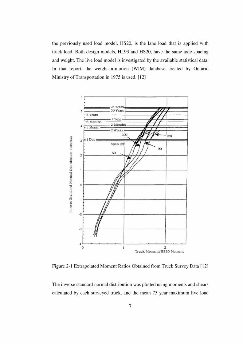
the previously used load model, HS20, is the lane load that is applied with
truck load. Both design models, HL93 and HS20, have the same axle spacing
and weight. The live load model is investigated by the available statistical data.
In that report, the weight-in-motion (WIM) database created by Ontario
Ministry of Transportation in 1975 is used. [12]
Figure 2-1 Extrapolated Moment Ratios Obtained from Truck Survey Data [12]
The inverse standard normal distribution was plotted using moments and shears
calculated by each surveyed truck, and the mean 75 year maximum live load
8
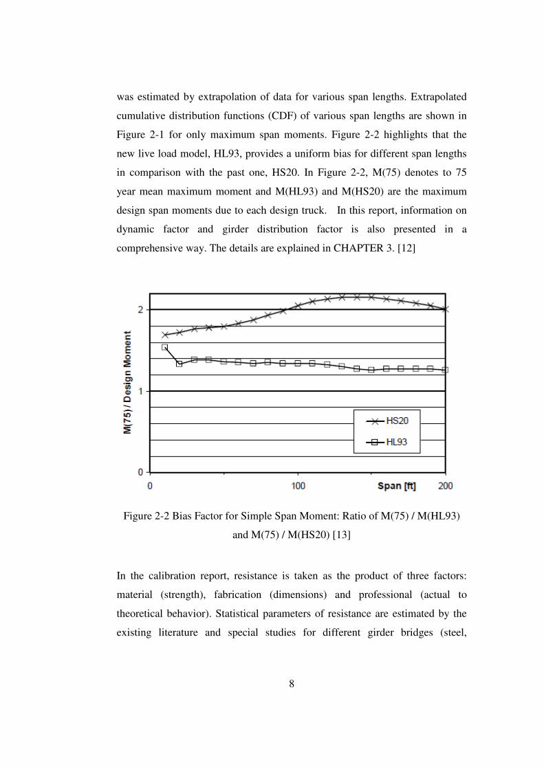
was estimated by extrapolation of data for various span lengths. Extrapolated
cumulative distribution functions (CDF) of various span lengths are shown in
Figure 2-1 for only maximum span moments. Figure 2-2 highlights that the
new live load model, HL93, provides a uniform bias for different span lengths
in comparison with the past one, HS20. In Figure 2-2, M(75) denotes to 75
year mean maximum moment and M(HL93) and M(HS20) are the maximum
design span moments due to each design truck. In this report, information on
dynamic factor and girder distribution factor is also presented in a
comprehensive way. The details are explained in CHAPTER 3. [12]
Figure 2-2 Bias Factor for Simple Span Moment: Ratio of M(75) / M(HL93)
and M(75) / M(HS20) [13]
In the calibration report, resistance is taken as the product of three factors:
material (strength), fabrication (dimensions) and professional (actual to
theoretical behavior). Statistical parameters of resistance are estimated by the
existing literature and special studies for different girder bridges (steel,
9
reinforced concrete and prestressed concrete). Resistance is taken as a
lognormal variate. [12]
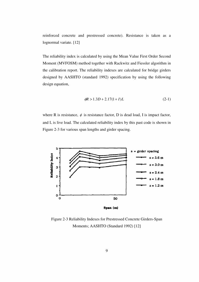
The reliability index is calculated by using the Mean Value First Order Second
Moment (MVFOSM) method together with Rackwitz and Fiessler algorithm in
the calibration report. The reliability indexes are calculated for bridge girders
designed by AASHTO (standard 1992) specification by using the following
design equation,
LIDR )1(17.23.1 ++>φ (2-1)
where R is resistance, φ is resistance factor, D is dead load, I is impact factor,
and L is live load. The calculated reliability index by this past code is shown in
Figure 2-3 for various span lengths and girder spacing.
Figure 2-3 Reliability Indexes for Prestressed Concrete Girders-Span
Moments; AASHTO (Standard 1992) [12]

10
The reliability index calculated by the previous AASHTO specifications
(Standard 1992) is not uniform and changes considerably by the spacing
between girders. Thus, the load and resistance factors are calibrated to achieve
a uniform safety level for all spans. In the calibration report, various load and
resistance factors were tried to be taken up to the target reliability level, as
displayed in Figure 2-4. In calibration of AASHTO LRFD Specifications, the
target reliability level is taken as 3.5. Therefore, after calibration, the design
equation becomes
LIDDR A )1(75.15.125.1 +++>φ (2-2)
where, R is resistance, φ is resistance factor (1.0 for moment and prestressed
concrete girders), D is dead load, AD is the dead load due to asphalt, I is
impact factor and L is live load.
By the new code (current) the dead load has been divided into two different
load components: weight of structural components and weight of wearing
surface. Dead load due to the asphalt has higher load factor because it involves
higher uncertainty. Another revision in the new code is the formulation of
girder distribution factor. The new expression minimizes the reliability index
changes due to girder spacing. As indicated in Figure 2-4, the new load and
resistance factors provide a uniform reliability level throughout a wide
spectrum of spans.

11
Figure 2-4 Reliability Indexes for Prestressed Concrete Girders-Span
Moments; Proposed LRFD Code (Current AASHTO LRFD) [12]
Another report [13] was published in 2007 to update the previously presented
report, NCHRP Report 368. This report summarizes the report of calibration of
LRFD bridge design code and presents procedures for collecting data. What
lacked in the previous report is explained. Indeed, in the previous report, the
reliability indexes were calculated by an iterative procedure (Rackwitz and
Fiessler). In this method, the non-normal variables are approximated to
equivalent normal variables by satisfying certain requirements. However, this
report suggests Monte Carlo Simulation technique to calculate the reliability
index because this procedure eliminates the need to approximate the
distribution. [13]
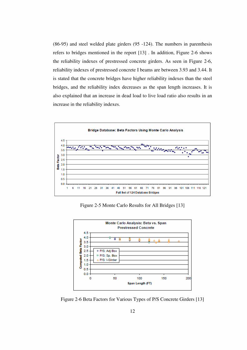
In updating the calibration report, the reliability index of girders of the 124
bridges designed by AASHTO LRFD Specifications is estimated by Monte
Carlo simulation. Figure 2-5 shows the reliability indexes of all types of
bridges: Prestressed concrete boxes (1-45), “California” prestressed concrete
boxes (46-51), prestressed concrete I-Beams (51-85), reinforced concrete slabs
12
(86-95) and steel welded plate girders (95 -124). The numbers in parenthesis
refers to bridges mentioned in the report [13] . In addition, Figure 2-6 shows
the reliability indexes of prestressed concrete girders. As seen in Figure 2-6,
reliability indexes of prestressed concrete I beams are between 3.93 and 3.44. It
is stated that the concrete bridges have higher reliability indexes than the steel
bridges, and the reliability index decreases as the span length increases. It is
also explained that an increase in dead load to live load ratio also results in an
increase in the reliability indexes.
Figure 2-5 Monte Carlo Results for All Bridges [13]
Figure 2-6 Beta Factors for Various Types of P/S Concrete Girders [13]

13
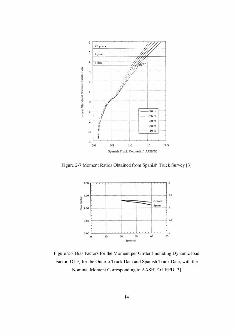
Another study carried out by Nowak et al. [3] compares the reliability level of
girders designed by Spanish Norma, Eurocode and AASHTO LRFD code.
Typical precast girders used in Spain are considered. The statistical parameters
used in the study are generally based on the previously explained calibration
report. In reliability analysis, statistical parameters of Spanish truck survey
and Ontario truck survey (used in calibration of AASHTO LRFD) are
considered. Extrapolated CDF of Spanish truck data is displayed in Figure 2-7.
It is stated that the cumulative distribution function (CDF) of moments is
assumed to follow an extreme type I (Gumbel) distribution, but it is
approximated to normal distribution; in particular this applies to the upper tail
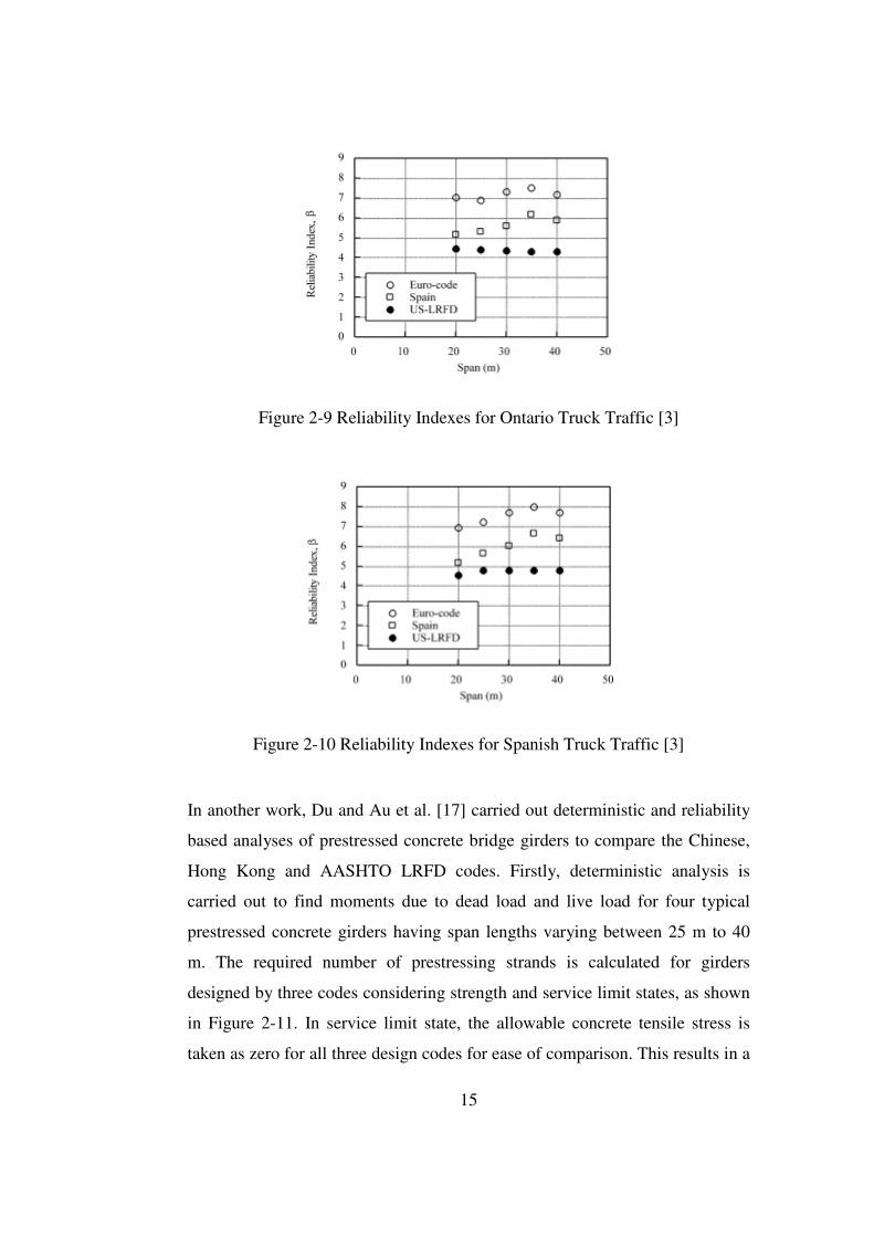
of CDF. Bias factor for both truck data is shown in Figure 2-8. An iterative
procedure is used estimating the reliability index as described by Rackwitz and
Fiessler. Reliability analysis is done for both Ontario and Spanish truck data as
shown in Figure 2-9 and Figure 2-10. The reliability indexes calculated based
on Spanish truck data are higher than those calculated based on Ontario truck
data. The results show that Eurocode is the most conservative one and
AASHTO LRFD is the most permissive code, and AASHTO LRFD provides
the most uniform safety level. [3]
14
Figure 2-7 Moment Ratios Obtained from Spanish Truck Survey [3]
Figure 2-8 Bias Factors for the Moment per Girder (including Dynamic load
Factor, DLF) for the Ontario Truck Data and Spanish Truck Data, with the
Nominal Moment Corresponding to AASHTO LRFD [3]
15
Figure 2-9 Reliability Indexes for Ontario Truck Traffic [3]
Figure 2-10 Reliability Indexes for Spanish Truck Traffic [3]
In another work, Du and Au et al. [17] carried out deterministic and reliability
based analyses of prestressed concrete bridge girders to compare the Chinese,
Hong Kong and AASHTO LRFD codes. Firstly, deterministic analysis is
carried out to find moments due to dead load and live load for four typical
prestressed concrete girders having span lengths varying between 25 m to 40
m. The required number of prestressing strands is calculated for girders
designed by three codes considering strength and service limit states, as shown
in Figure 2-11. In service limit state, the allowable concrete tensile stress is
taken as zero for all three design codes for ease of comparison. This results in a
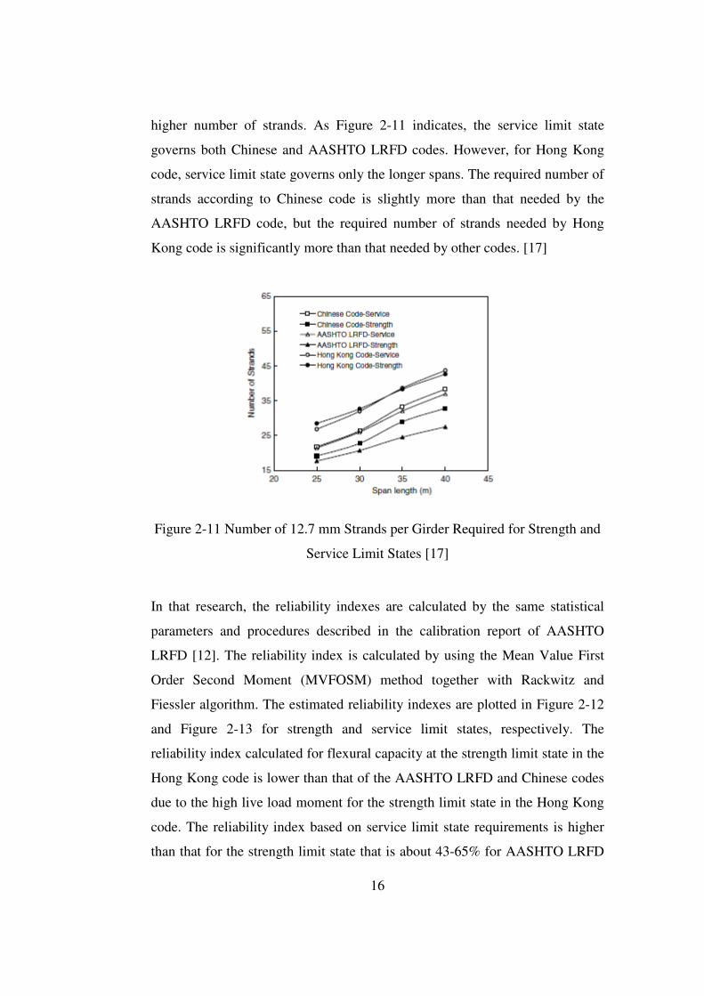
16
higher number of strands. As Figure 2-11 indicates, the service limit state
governs both Chinese and AASHTO LRFD codes. However, for Hong Kong
code, service limit state governs only the longer spans. The required number of
strands according to Chinese code is slightly more than that needed by the
AASHTO LRFD code, but the required number of strands needed by Hong
Kong code is significantly more than that needed by other codes. [17]
Figure 2-11 Number of 12.7 mm Strands per Girder Required for Strength and
Service Limit States [17]
In that research, the reliability indexes are calculated by the same statistical
parameters and procedures described in the calibration report of AASHTO
LRFD [12]. The reliability index is calculated by using the Mean Value First
Order Second Moment (MVFOSM) method together with Rackwitz and
Fiessler algorithm. The estimated reliability indexes are plotted in Figure 2-12
and Figure 2-13 for strength and service limit states, respectively. The
reliability index calculated for flexural capacity at the strength limit state in the
Hong Kong code is lower than that of the AASHTO LRFD and Chinese codes
due to the high live load moment for the strength limit state in the Hong Kong
code. The reliability index based on service limit state requirements is higher
than that for the strength limit state that is about 43-65% for AASHTO LRFD

17
code, 83-103% for Hong Kong code, and 23-30% for Chinese code. The
reliability indexes of service limit state are fairly close to one another for all of
the three codes. [17]
Figure 2-12 Reliability Indexes for Flexural Capacity Based on the
Requirements of the Strength Limit State in the Three Codes [17]
Figure 2-13 Reliability Indexes for Flexural Capacity Based on the
Requirements of the Service Limit State in the Three Codes [17]

18
CHAPTER 3
STATISTICS OF LOAD
3.1 DESIGN LIMIT STATES AND LOAD COMBINATIONS
The following limit states are specified in AASHTO LRFD Specifications
(AASHTO LRFD 3.4.1) to design components and connections of a bridge [1];
• Strength I – Basic load combination relating to the normal vehicular use
of the bridge without wind.
• Strength II – Load combination relating to the use of the bridge by
owner-specified special design vehicles, evaluation permit vehicles, or
both without wind.
• Strength III – Load combination relating to the bridge exposed to wind
velocity exceeding 55 mph.
• Strength IV – Load combination relating to very high dead load to live
load force effect ratios.
• Strength V – Load combination relating to normal vehicular use of the
bridge with wind of 55 mph velocity.
• Extreme Event I – load combination including earthquake.

19
• Extreme Event II – load combination relating to ice load, collision by
vessels and vehicles, and certain hydraulic events with a reduced live
load other than that which is part of the vehicular collision load.
• Service I – Load combination relating to the normal operational use of
the bridge with a 55 mph wind and all loads taken at their nominal
values.
• Service II – load combination intended to control yielding of steel
structures and slip of slip-critical connections due to vehicular live load.
• Service III – Load combination for longitudinal analysis relating to
tension in prestressed concrete superstructures with the objective of
crack control and to principal tension in the webs of segmental concrete
girders.
• Service IV – Load combination relating only to tension in prestressed
concrete columns with the objective of crack control.
• Fatigue – fatigue and fracture load combination relating to repetitive
gravitational vehicular live load and dynamic responses under a single
design truck.
The design of prestressed beams usually needs to be checked against the
requirements of Service I, Service III and Strength I limit states [2]. Service I
checks the compression stress, and Service III checks the tensile stress in
prestressed concrete component at the critical section and critical top or bottom
fiber. Strength I is used to estimate the ultimate strength. In designing
prestressed beam, typically Service III governs and controls the design in terms
of the determining number of prestressing steel for a selected cross-section. In
20
a typical prestressed bridge girder design, industry accepted span to depth
ratios are used to select the depth of girder and corresponding shelf cross-
section. The cracking at bridge girders is the most unwanted situation since the
bridge girders cannot be protected adequately from environmental conditions.
Typically, cracking of concrete is controlled by limiting the tension stress of
concrete fibers.
The reliability analysis of prestressed concrete girders is carried out for the
Strength I Limit state that is set to ensure that bridge itself or its elements will
have certain strength and stability to resist the specified statistically significant
gravity load combination that a bridge could be subjected during its economic
life. Reliability analysis for Service III limit state is also evaluated to ensure
that bridge will continue to maintain a certain level of durability and passenger
comfort under statistically determined gravity loads and load combinations
while in use.
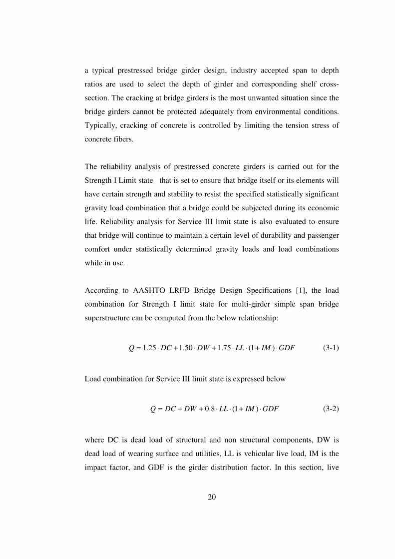
According to AASHTO LRFD Bridge Design Specifications [1], the load
combination for Strength I limit state for multi-girder simple span bridge
superstructure can be computed from the below relationship:
GDFIMLLDWDCQ ⋅+⋅⋅+⋅+⋅= )1(75.150.125.1 (3-1)
Load combination for Service III limit state is expressed below
GDFIMLLDWDCQ ⋅+⋅⋅++= )1(8.0 (3-2)
where DC is dead load of structural and non structural components, DW is
dead load of wearing surface and utilities, LL is vehicular live load, IM is the
impact factor, and GDF is the girder distribution factor. In this section, live

21
load including truck load, lane load, impact factor and girder distribution factor
and dead load will be identified, and related uncertainties due to these load
components will be assessed.
3.2 DEAD LOAD
The dead load consists of four components:
1D - Weight of factory made elements (steel and precast beams)
2D - Weight of cast-in-place concrete (deck)
3D -Weight of wearing surface (asphalt)
4D - Weight of miscellaneous (railing, luminaries).
In strength I limit state, the load factor for weight of factory prepared elements,
1D , and cast-in-place concrete components, 2D , are set to 1.25, and the load
factor for wearing surface, 3D , and miscellaneous items, 4D , are set to 1.5.
In this study, statistical parameters of dead load components are taken from
Nowak’s study [13]. All dead load variables are considered to be normally
distributed. The wearing surface, i.e. the asphalt layer, has the highest
uncertainty among the dead load components. For miscellaneous components,
the bias factor and coefficient of variation can vary, but in this study, these
values are taken as 1.05 and 0.10, respectively to stay on the conservative side.
Mean bias factor is the ratio of the mean of true value to nominal value.
(Increase in the bias factor and coefficient of variation for load components
typically results in lower reliability indexes.)

22
Table 3-1 Statistical Parameters of Dead Load from Nowak et al. [12]
Dead Load Component Bias Factor Coefficient of Variation
Factory Made Members,D1 1.03 0.08
Cast-in-place,D2 1.05 0.1
Wearing Surface,D3 1 0.25
Miscellaneous,D4 1.03~1.05 0.08~0.10
3.3 LIVE LOAD
3.3.1 Live Load Models
In this section, live load model of AASHTO LRFD, HL-93, and the live load
model of Turkey, H30-S24 will be introduced, and the span moment due to
both HL-93 and H30-S24 loading will be presented.
3.3.1.1 HL-93 Loading
The live load model of AASHTO LRFD Bridge Design specifications consists
of a combination of
• Design truck or design tandem, and
• Design lane.
HL-93 truck model is used as the design truck. The weights and spacings of
axles and wheels for the design truck are specified in Figure 3-1. The spacing
between the two back axles is varied from 4.3 m to 9.0 m to produce the
maximum load effect. The width of loads for a single lane is assumed to
occupy 3000 mm [1].

23
The design tandem consists of a pair of 110000 N axles spaced 1200 mm apart
and the transverse spacing of wheels is taken as 1800 mm. Design lane load
consists of a load of 9.3 N/mm uniformly distributed in the longitudinal
direction, and it is assumed to be uniformly distributed over 3000 mm
width.[1]
In order to obtain the extreme force effect, the effects of an axle sequence and
the lane load are superposed. Extreme force effect is taken as the larger of the
following:
Figure 3-1 Characteristics of Design Truck, HL-93
i. the effect of one design truck with the variable axle spacing combined
with the effect of the design lane load ( as shown in Figure 3-2.a),
ii. the effect of the design tandem combined with the effect of the design
lane load (as shown in Figure 3-2.b),
24
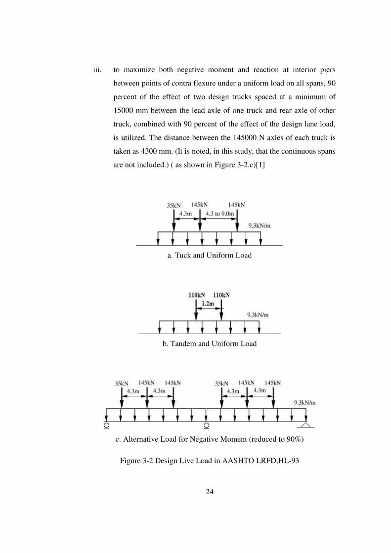
iii. to maximize both negative moment and reaction at interior piers
between points of contra flexure under a uniform load on all spans, 90
percent of the effect of two design trucks spaced at a minimum of
15000 mm between the lead axle of one truck and rear axle of other
truck, combined with 90 percent of the effect of the design lane load,
is utilized. The distance between the 145000 N axles of each truck is
taken as 4300 mm. (It is noted, in this study, that the continuous spans
are not included.) ( as shown in Figure 3-2.c)[1]
a. Tuck and Uniform Load
b. Tandem and Uniform Load
c. Alternative Load for Negative Moment (reduced to 90%)
Figure 3-2 Design Live Load in AASHTO LRFD,HL-93

25
3.3.1.2 H30-S24 Loading
The live load model consisting of design truck load and design lane load with
concentrated load is specified in the Technical Specifications for Roads and
Bridges in Turkey [14]. H30-S24 is specified as a design truck, the weights and
spacings of axles and wheels for the design truck are depicted in Figure 3-3.
Gross weight of H30-S24 truck is 600 kN. Concentrated loads are usually
combined with design lane load to develop maximum moment and shear effect
along the superstructure. Similar to HL-93 truck, effective load width for a
single lane can be assumed as 3000 mm. Extreme force effect is taken as the
larger of the following:
i.The maximum effect of one design truck ( as shown in Figure 3-4.a),
ii.The maximum effect of the design lane load combined with
concentrated load (as shown in Figure 3-4.b).
Figure 3-3 Characteristics of Design Truck, H30-S24

26
a. Only Truck Load
b. Lane and Concentrated Load
Figure 3-4 Design Live Load in Turkey, H30-S24 [14]
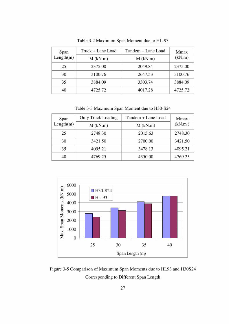
3.3.1.3 Maximum Span Moments due to HL-93 and H30-S24
The maximum mid-span moments were calculated by determining the
optimum position of the truck model on the span that will develop the
maximum load effect on the mid-span. Results for HL-93 and H30-S24 are
tabulated and shown in Table 3-2 and Table 3-3, respectively. HL-93 will mean
the load effect per maximum of truck load with lane load and tandem load, and
H30-S24 will mean the load effect per maximum of only truck load and
tandem with lane load, throughout this thesis. As the results indicate, tandem
loads do not result in the maximum span moments. Moreover, the maximum
span moment due to H30-S24 is approximately 10% higher due to HL-93.
However, the difference in maximum moment decreases as the span length
increases. This decrease is caused by the additional lane load with truck
loading in HL-93. Figure 3-5 indicates the difference between both loadings.
27
Table 3-2 Maximum Span Moment due to HL-93
Table 3-3 Maximum Span Moment due to H30-S24
Only Truck Loading Tandem + Lane Load Span Length(m) M (kN.m) M (kN.m)
Mmax (kN.m )
25 2748.30 2015.63 2748.30
30 3421.50 2700.00 3421.50
35 4095.21 3478.13 4095.21
40 4769.25 4350.00 4769.25
0
1000
2000
3000
4000
5000
6000
25 30 35 40
Span Length (m)
Max
. Spa
n M
omen
ts (
kN.m
) .
H30-S24
HL-93
Figure 3-5 Comparison of Maximum Span Moments due to HL93 and H30S24
Corresponding to Different Span Length
Truck + Lane Load Tandem + Lane Load Span Length(m) M (kN.m) M (kN.m)
Mmax (kN.m)
25 2375.00 2049.84 2375.00
30 3100.76 2647.53 3100.76
35 3884.09 3303.74 3884.09
40 4725.72 4017.28 4725.72

28
3.3.2 Evaluation of Truck Survey Data
The truck survey data was gathered from the Turkish General Directorate of
Highways to evaluate the statistical parameters of live load in Turkey. This
survey data was examined and the suspicious measurements (i.e. measurements
with possible errors) were deleted to carry out more accurate statistical
analysis. The maximum span moments due to surveyed trucks were calculated
in this chapter.
3.3.2.1 Truck Survey Data
In Turkey, truck-survey programs have been carried out by the General
Directorate of Highways. Division of Transportation and Cost Studies under
the Department of Strategy Development is responsible for carrying out site
measurements and collecting data. Site measurements are done at any selected
station of highways throughout the year. These measurements are referred to as
“Axle Weight Studies”. Every year, this study is conducted at over 40 stations
and covers a total of nearly 15000 vehicles.
Department of Strategy Development works on this data and on other
transportation surveys to produce statistical information about the highways of
Turkey. Results of these surveys assist the experts in making decisions about
the future of highways and planning and managing the facilities. After the
evaluation of data obtained from the traffic survey, reports are published every
year.
Axle Weight Studies are carried out on highways. The officials locate a
selected station on the highways. They control the vehicles by stopping them
randomly. It is similar to traffic police controls. Not only the heavy trucks but
also the buses, vans, empty trucks, trailers are stopped, and measurements are
29
taken. Name and kilometers of location, weight of each axle, type of truck axle,
type and model of vehicles are recorded during these site studies.
In order to examine the statistical parameters of live load on bridges in Turkey,
Axle Weight Studies were carried out by the Division of Transportation and
Cost Studies. A survey on trucks provides data belonging to years 1997-2006,
and a part of this data is presented in Table 3-4.
Notations are used to classify the vehicles according to axle types. A list of
notations used in this survey is presented in Table 3-5. In this table, 15
different notations are shown. The notation which is in parentheses has the
same axle configuration with the other, but has different tire numbers. One of
the example notations is illustrated in Figure 3-6. Each number indicates the
axles. That is, “1” indicates that there is one tire on each side, and “2” indicates
that there are two tires on each side. A point in notation is used for dividing
front axles from back axles. The numbers that are to the left of the point are the
front axles of vehicle, and followings are the back axles. The types of vehicles
are noted at the truck survey. These types are shown in Table 3-6.

30
Table 3-4 Partial Sample Data for Axle Weight Measurements (BABAESKĐ-
LÜLEBURGAZ Direction) [24]
SNO YON TCIN NETAG ISHAD TMAR TTIP TMOD YCIN GELY GITY KM DTIP D1 D2 D3 D4 D5 D6
1 1 2 8890 16110 MERCEDES 2523 04 1 39 59 93 1.22 2.30 4.20 0.00 0.00 0.00 0.00
2 1 1 6025 33 MITSUBISHI POWERS 06 30 39 59 120 1.2 0.00 0.00 0.00 0.00 0.00 0.00
3 1 2 3900 4600 IVECO 80-12 01 5 39 39 23 1.2 1.70 3.60 0.00 0.00 0.00 0.00
4 1 2 11000 22000 BMC PRO822 00 2 39 6 618 11.22 2.80 4.10 6.90 4.90 0.00 0.00
5 1 2 5100 6540 MAN 12.163 04 6 39 59 93 1.22 1.40 1.60 1.50 0.00 0.00 0.00
6 1 2 3140 219 ISUZU NKR 66 05 6 22 59 139 1.2 0.90 2.10 0.00 0.00 0.00 0.00
7 1 2 8120 17380 FORD 2520 97 1 59 39 123 1.22 1.40 2.00 1.10 0.00 0.00 0.00
8 1 2 3110 390 ISUZU NKR 66 99 6 22 39 84 1.2 1.10 1.90 0.00 0.00 0.00 0.00
9 1 2 4027 3673 MITSUBISHI 659 04 9 39 39 23 1.2 1.50 1.90 0.00 0.00 0.00 0.00
10 1 1 5920 27 OTOKAR N 145 06 10 39 59 120 1.2 0.00 0.00 0.00 0.00 0.00 0.00
11 1 1 6551 31 ISUZU TURKUAZ 05 2 22 59 139 1.2 0.00 0.00 0.00 0.00 0.00 0.00
12 1 2 1730 1150 KIA K 2500 04 4 39 39 62 1.2 0.60 0.90 0.00 0.00 0.00 0.00
13 1 3 14200 28050 MAN 19-422 99 1 39 39 23 1.2+222 2.90 2.80 0.00 2.60 1.90 0.00
14 1 2 7950 17550 FORD 2520 92 1 22 39 71 1.22 1.70 1.70 1.40 0.00 0.00 0.00
15 1 2 9510 16490 FARGO 26-200 95 6 39 34 181 1.22 3.00 6.10 5.00 0.00 0.00 0.00
16 1 2 4110 2890 MITSUBISHI FE 449 92 6 39 34 209 1.2 1.10 1.80 0.00 0.00 0.00 0.00
17 1 1 13700 46 MITSIBUSHI MS 827 01 22 22 34 236 1.2 0.00 0.00 0.00 0.00 0.00 0.00
18 1 3 14400 24600 MERCEDES 1840 05 1 39 59 93 1.2+111 2.80 2.80 0.00 1.90 1.80 0.00
19 1 2 10050 21950 FORD 3227 05 1 39 59 120 11.22 1.30 1.30 3.30 0.00 0.00 0.00
20 1 2 3627 3878 ISUZU NPR 66 00 9 39 39 23 1.2 1.50 4.20 0.00 0.00 0.00 0.00
21 1 2 8577 16423 MERCEDES 2523 04 1 39 59 93 1.22 2.50 2.60 1.70 0.00 0.00 0.00
22 1 1 13570 46 MERCEDES 0403 03 26 39 34 209 1.2 0.00 0.00 0.00 0.00 0.00 0.00
23 1 2 3627 3873 ISUZU NPR 66 00 9 39 39 23 1.2 1.40 4.40 0.00 0.00 0.00 0.00
24 1 2 8538 16462 MERCEDES 2521 94 9 22 41 328 1.22 2.70 3.50 3.40 0.00 0.00 0.00
25 1 2 7586 17414 FORD 2517 90 6 39 34 181 1.22 2.70 6.00 4.50 0.00 0.00 0.00
26 1 2 2250 950 IVECO 35-9 01 9 39 34 181 1.2 1.20 1.40 0.00 0.00 0.00 0.00
27 1 2 2125 1378 IVECO 35-10 01 9 39 39 62 1.2 0.90 1.40 0.00 0.00 0.00 0.00
28 1 1 6490 27 OTOKAR N 145-S 04 14 39 59 93 1.2 0.00 0.00 0.00 0.00 0.00 0.00
29 1 2 8640 16360 BMC 200-26 02 1 59 59 96 1.22 1.70 3.40 0.00 0.00 0.00 0.00
30 1 2 12850 19000 BMC PRO 827 03 2 59 39 89 11.22 4.20 2.70 7.70 5.30 0.00 0.00
31 1 2 10800 21200 FARGO 32-26 04 4 39 39 62 11.22 3.60 5.00 9.10 7.00 0.00 0.00
32 1 2 8400 16600 BMC 200-264 98 9 59 39 89 1.22 2.60 3.40 1.90 0.00 0.00 0.00
33 1 2 8040 16949 FORD 2520 03 1 39 39 120 1.22 1.70 3.40 0.00 0.00 0.00 0.00
34 1 2 13250 12235 IVECO 330-30 96 4 39 39 23 1.22 3.10 3.20 3.00 0.00 0.00 0.00
35 1 2 12110 13900 IVECO 330-30 93 4 39 39 23 1.22 3.60 5.70 5.30 0.00 0.00 0.00
36 1 3 14700 32600 MERCEDES 1840 05 1 39 39 23 1.2+111 2.80 2.90 0.00 2.00 1.60 0.00
37 1 2 13250 12235 IVECO 330-30 95 4 39 39 23 1.22 2.50 2.80 2.90 0.00 0.00 0.00
38 1 2 10000 15000 MERCEDES 2500 98 4 39 39 93 1.22 3.90 7.90 6.10 0.00 0.00 0.00
39 1 2 10150 21700 MERCEDES 3228 05 1 39 59 71 11.22 2.10 0.00 3.70 0.00 0.00 0.00
40 1 2 1225 4775 MITSUBISHI AE 449 97 1 39 39 23 1.2 2.10 1.80 1.80 0.00 0.00 0.00
41 1 2 9000 16000 FORD 2217 89 1 22 39 139 1.22 1.90 1.50 1.10 0.00 0.00 0.00
42 1 3 15100 28710 MERCEDES 1840 04 1 22 39 159 1.2+111 2.70 2.40 0.00 1.80 1.65 0.00
43 1 2 6950 14050 FORD 2014 89 4 39 39 93 1.21 2.00 7.10 2.30 0.00 0.00 0.00
44 1 2 8990 16010 BMC PRO 620 00 1 22 39 68 1.22 2.40 2.20 1.80 0.00 0.00 0.00
45 1 2 12540 13460 MERCEDES 3028 04 4 39 39 23 1.22 3.20 5.20 5.00 0.00 0.00 0.00
46 1 2 3100 3900 MITSUBISHI 449 97 1 22 39 68 1.2 0.80 1.40 0.00 0.00 0.00 0.00
47 1 2 12010 19990 BMC PRO 822 02 5 39 39 23 11.22 3.80 0.00 5.50 3.50 0.00 0.00
48 1 1 5600 29 OTOKAR 145,5 04 10 39 59 120 1.2 0.00 0.00 0.00 0.00 0.00 0.00
49 1 2 6900 17030 BMC FATİH 145-22 88 2 59 39 99 1.22 2.90 6.60 4.60 0.00 0.00 0.00
50 1 1 4300 23 IVECO M 23 97 2 39 39 23 1.2 0.00 0.00 0.00 0.00 0.00 0.00
51 1 2 10500 21500 FORD 32-20 06 2 39 6 618 11.22 4.10 0.00 8.20 6.20 0.00 0.00
52 1 3 15110 25100 MERCEDES 1840 04 5 59 34 153 1.2+111 3.30 5.60 2.90 2.90 2.90 0.00
53 1 3 15050 28050 MAN 26-321 78 1 59 34 196 1.2+22 2.50 2.10 2.20 1.20 0.00 0.00
54 1 2 4160 3340 MITSUBISHI 659 98 1 39 39 23 1.2 0.90 1.30 0.00 0.00 0.00 0.00
55 1 2 1950 1250 KIA K 2500 05 9 22 59 139 1.2 0.60 0.70 0.00 0.00 0.00 0.00
56 1 2 6800 16300 MERCEDES 1517 01 1 22 39 84 1.22 1.80 1.40 1.40 0.00 0.00 0.00
57 1 3 14100 28200 DAF 85-400 95 2 22 59 127 1.2+111 3.30 6.60 4.80 4.70 4.20 0.00
58 1 2 5525 16975 VOLVO F 10 91 9 39 39 23 1.22 1.50 4.60 4.60 0.00 0.00 0.00
59 1 1 6025 33 MITSUBISHI POWERP 06 20 39 59 93 1.2 0.00 0.00 0.00 0.00 0.00 0.00
60 1 1 6000 30 MERCEDES 05 28 39 59 93 1.2 0.00 0.00 0.00 0.00 0.00 0.00
61 1 2 9000 23000 SCANIA 94-GB 01 2 39 26 500 11.22 2.40 2.80 6.20 5.80 0.00 0.00
62 1 2 7490 15610 MERCEDES 15-17 04 1 39 59 120 1.22 1.30 3.20 0.00 0.00 0.00 0.00
63 1 2 10320 15180 MERCEDES 25 17 91 1 22 39 71 1.22 2.20 2.20 1.40 0.00 0.00 0.00
64 1 2 2920 580 MITSIBUSHI 639 05 5 59 59 67 1.2 1.00 1.50 0.00 0.00 0.00 0.00
65 1 2 12050 19950 FARGO AS 32 05 4 22 39 84 11.22 3.00 3.40 5.90 4.90 0.00 0.00
66 1 2 6000 9000 MERCEDES 1517 05 9 59 39 68 1.2 1.90 2.40 0.00 0.00 0.00 0.00
67 1 2 2900 500 MERCEDES 06 1 900 34 250 1.1 0.90 1.20 0.00 0.00 0.00 0.00
68 1 2 5480 6000 FARGO AS 32 05 1 59 39 34 11.22 1.00 1.80 0.50 0.30 0.00 0.00
69 1 2 9350 15650 DODGE AS 950 97 4 39 39 23 1.22 1.90 2.80 2.30 0.00 0.00 0.00
70 1 2 9965 15035 MERCEDES 2523 06 1 39 59 93 1.22 2.30 2.40 1.90 0.00 0.00 0.00
71 1 2 5060 7040 ISUZU NOR 30 04 1 22 59 139 1.21 1.20 1.30 0.50 0.00 0.00 0.00
72 1 2 2301 5399 MITSUBISHI FE659 00 9 39 39 23 1.2 1.30 3.10 0.00 0.00 0.00 0.00
73 1 1 6551 31 ISIZU TURZ 31 04 14 22 59 139 1.2 0.00 0.00 0.00 0.00 0.00 0.00
74 1 2 2300 950 DODGE 200 97 9 39 39 23 1.1 0.90 1.30 0.00 0.00 0.00 0.00

31
Table 3-5 Notation of Axle Types
1.1 1.2+2
1.2 1.2+21
1.21
1.2+11 (1.2+22)
1.22
1.22+11 (1.22+22)
1.121 (1.122)
1.2+111
11.21
1.2+122 (1.2+222)
11.22
1.22+111 (1.22+222)
Figure 3-6 Example of Axle Type Notation
Table 3-6 Vehicle Type
Type No Type Name
1 Truck
2 Truck + Trailer
3 Wrecker
4 Wrecker + Half Trailer
5 Bus

32
3.3.2.2 The Span Moments due to Surveyed Trucks
The last two years of measurements of a ten-year data covering axle weight
measurements was used to carry out statistical evaluations. Manufacturers
design more efficient vehicles using new technologies in order to better
respond to the increasing demand. Vehicle configurations and load carrying
capacities have changed over the years. Therefore, to reflect today’s vehicle
configurations, the past survey results were ignored, but only truck
measurements of the years 2005 and 2006 were considered in this study.
Figure 3-7 Histogram of Vehicles according to Axle Types
Data covering the two years have more than 20.000 records of vehicles. Figure
3-7 shows the variation of vehicle numbers according to the axle types. Also,
note that the numbers in parenthesis denote the type of vehicle as presented in
33
Table 3-6. The truck having three axles, “1.22” is observed to be the most
common vehicle in the survey.
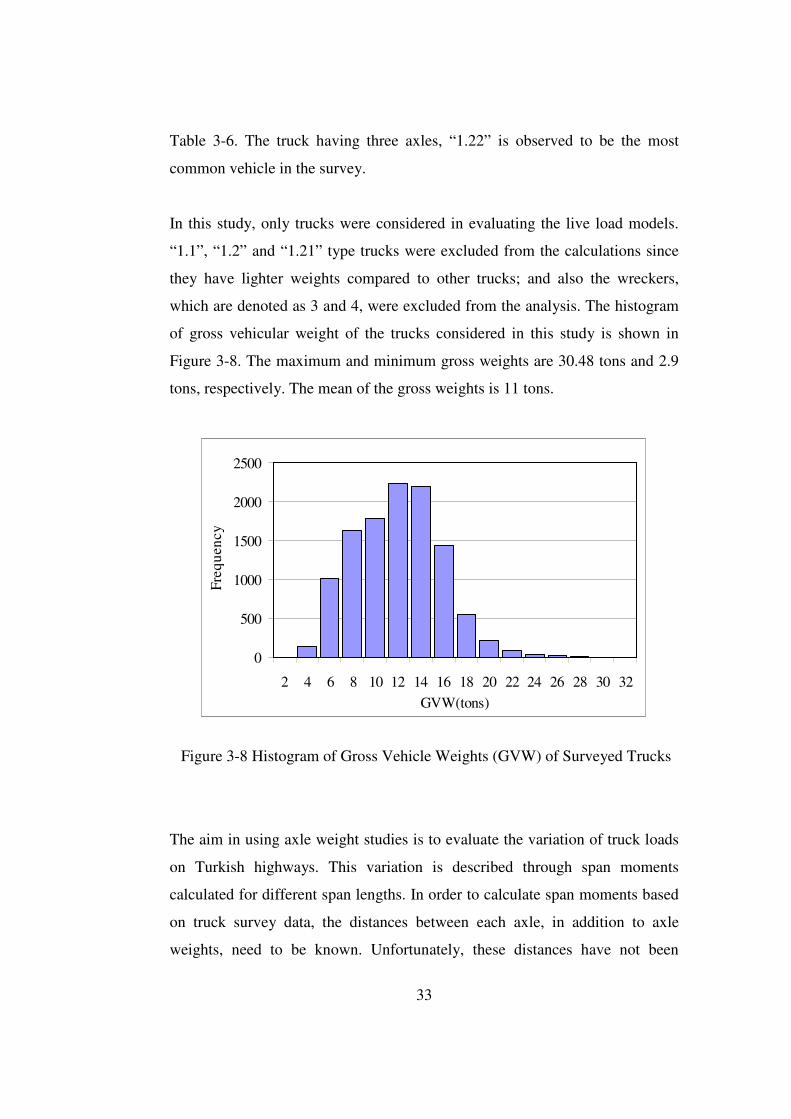
In this study, only trucks were considered in evaluating the live load models.
“1.1”, “1.2” and “1.21” type trucks were excluded from the calculations since
they have lighter weights compared to other trucks; and also the wreckers,
which are denoted as 3 and 4, were excluded from the analysis. The histogram
of gross vehicular weight of the trucks considered in this study is shown in
Figure 3-8. The maximum and minimum gross weights are 30.48 tons and 2.9
tons, respectively. The mean of the gross weights is 11 tons.
0
500
1000
1500
2000
2500
2 4 6 8 10 12 14 16 18 20 22 24 26 28 30 32
GVW(tons)
Fre
qu
ency
Figure 3-8 Histogram of Gross Vehicle Weights (GVW) of Surveyed Trucks
The aim in using axle weight studies is to evaluate the variation of truck loads
on Turkish highways. This variation is described through span moments
calculated for different span lengths. In order to calculate span moments based
on truck survey data, the distances between each axle, in addition to axle
weights, need to be known. Unfortunately, these distances have not been

34
measured in the axle weight studies. For this reason, these distances are
assumed according to catalog search for each truck type. The truck catalogs of
manufacturers are obtained from their web sites. The distances between axles
are taken from these catalogs, and then the range of these distances is
determined for each truck type as shown in Table 3-7 within parenthesis.
Generally, the shortest distances from these ranges are assumed for the
distances between axles for each truck type, and these distances are used for
every truck of corresponding types. In some cases, the most common axle
distance is taken. It should be noted that using the shortest axle distances
results in high moments induced by truck passages over the spans.
Table 3-7 Assumed Truck Axle Distances
Distance between Each Axles (m) Truck Type
D1-D2 D2-D3 D3-D4
1.21 and 1.22 3.80
(3.60 ≤ 5.00 ) 1.35
(1.15 ≤ 1.40 ) -
11.22 1.70
(1.70 ≤ 1.95 ) 2.80
(2.80 ≤ 3.40 ) -
1.121 3.80
(3.80 ≤ 5.00 ) 1.35
(1.15 ≤ 1.40 ) 1.35
(1.15 ≤ 1.40 )
Where, D: Axle (D1 is the front axle, D2 is the back axle)
Axle weights of nearly 11000 trucks were used in moment calculations. For
each truck, the bending moment was calculated by using assumed truck axle
distances for each type (Table 3-7), and they were determined separately for
the span lengths of which are 25 m, 30 m, 35 m, 40 m. The macro algorithm
was developed at Excel to calculate each truck load effect. Maximum moments
due to truck survey data were evaluated by moving the axle weight of each
truck on simple beam model at 0.25 m increment. For each increment, the
maximum moment was determined and stored. After all axles of each truck

35
passed through whole length of the span, the maximum moment due to this
truck was calculated by taking the maximum of stored moments. Histograms of
calculated surveyed tuck moment are plotted in Figure 3-9 to Figure 3-12.
0.00
200.00
400.00
600.00
800.00
1000.00
1200.00
50 300
550
800
1050
1300
1550
1800
2050
2300
2550
2800
Surveyed Truck Span Moment (kN.m)
Fre
quen
cy .
Figure 3-9 Histogram of Surveyed Truck Span Moments for 25 m Span Length
0.00100.00200.00300.00400.00500.00600.00700.00800.00900.00
1000.00
50 300
550
800
1050
1300
1550
1800
2050
2300
2550
2800
Surveyed Truck Span Moment (kN.m)
Fre
quen
cy .
Figure 3-10 Histogram of Surveyed Truck Span Moments for 30 m Span
Length
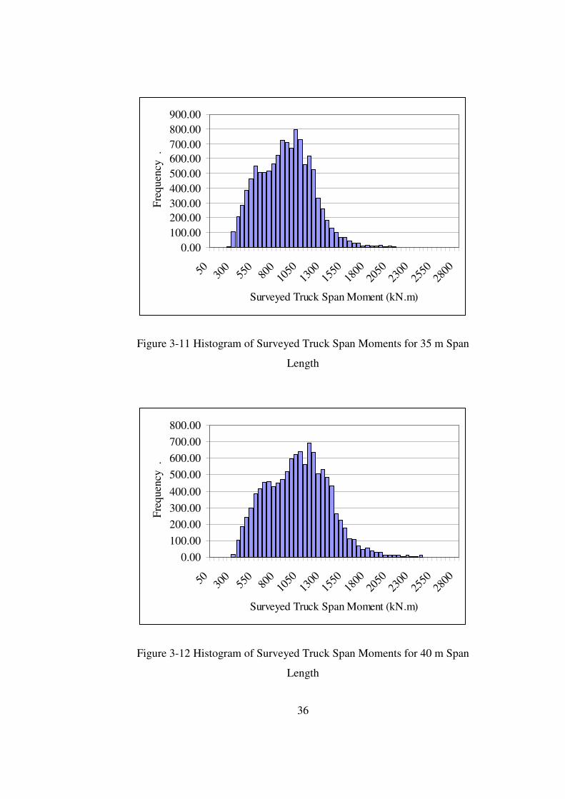
36
0.00100.00
200.00300.00400.00500.00600.00700.00
800.00900.00
50 300
550
800
1050
1300
1550
1800
2050
2300
2550
2800
Surveyed Truck Span Moment (kN.m)
Fre
quen
cy .
Figure 3-11 Histogram of Surveyed Truck Span Moments for 35 m Span
Length
0.00
100.00
200.00
300.00
400.00
500.00
600.00
700.00
800.00
50 300
550
800
1050
1300
1550
1800
2050
2300
2550
2800
Surveyed Truck Span Moment (kN.m)
Fre
quen
cy .
Figure 3-12 Histogram of Surveyed Truck Span Moments for 40 m Span
Length

37
3.3.2.3 Uncertainty Involved in the Truck Survey Data
Besides the inherent (aleatory) uncertainty evaluated previously, truck survey
data contains some errors and lacks information that causes prediction
(epistemic) uncertainties in the statistical evaluation of the data. These errors
are listed as follows:
• calibration of the weight measuring devices
• typing errors while performing the truck survey
• typing errors while transferring the truck survey measurements to
computer
• lack of axle distance
Some calibration errors may occur during field measurements. Calibration of
weight measuring devices is a very crucial part of site measurements to
determine the accurate weights.
Another type of error is the human error. While performing field
measurements, the value that is read from a weight measuring device is
sometimes typed on the paper incorrectly. In addition, some mistakes may be
made during the coding of field measurements into a computer program. Data
should be filtered from such errors to achieve more reliable statistical
estimations. For this purpose, axle weight measurements are examined row by
row visually to identify errors. The data considered to have typing errors are
deleted.
As previously mentioned, the axle weight measurements do not include axle
distances. These distances are assumed according to truck catalog searches.
Using assumed axle distances instead of using actual axle distances introduces
uncertainty into the span moment calculations.

38
Assuming shortest axle distances in moment calculations results in
conservative moments. Therefore, in this study, the additional uncertainties
related to the errors and assumptions previously mentioned are not taken into
account.
3.3.3 Assessment of the Statistical Parameters of Live Load
Statistical parameters of surveyed trucks are evaluated using the concepts
developed for extreme value theory. The main objective of this theory is to
extend the available data observed in shorter periods to longer periods by
extrapolation. In this study, maximum mean truck effects for longer time
periods are estimated by using this theory and assumptions set for calibration
of AASHTO LRFD [12].
Three different cases are evaluated to assess the statistical parameters to define
the live load; these are (1) overall surveyed trucks moments, where the original
truck survey data is kept except the suspicious ones (2) upper tail of cumulative
distribution functions of overall surveyed truck moments and (3) extreme
(maximum) surveyed truck moments. Overall surveyed truck moments are
calculated by using a total of 11000 axle truck loads as explained in section
3.3.2. Cumulative distribution functions of this overall data are plotted on
probability papers (Gumbel) to estimate the parameters of the probability
distribution. The maximum mean moments of future time periods are
determined by extrapolation of straight lines fitting to the curves. In the second
case, extrapolation of only the straight lines fitting to upper tail of the curves is
utilized. In the third case, statistical parameters of live load are estimated by
utilizing only the extreme truck moment values that is the highest 10% values
of overall surveyed truck moments. This corresponds to the values exceeding
the 90-percentile value of the original data. The third case is more
39
representative of extreme truck loads in the data set. In the rest of this thesis we
refer to these cases, respectively as overall, upper tail, and extreme.
3.3.3.1 Straight Lines Fitted to the CDFs of Surveyed Truck Moments
Cumulative distribution functions (CDFs) of overall surveyed truck moments
are plotted on both normal and Gumbel probability papers to examine the
goodness of fit of the data to these two probability distributions. After this
point, the moments are expressed as the ratio of surveyed truck moments to
corresponding design moments (maximum span moments are calculated
according to AASHTO LRFD for each live load model; H30S24 and HL93,
see Table 3-2 and Table 3-3).
Moment ratios of overall truck survey data are plotted on normal probability
papers in Figure 3-13 and Figure 3-14 for H30S24 and HL93 loadings. The
vertical scale in these figures is the inverse of the standard normal distribution
function (φ ), ISDN, denoted by z;
)]([1 MFz −= φ (3-3)
where, M is the span moment, F(M) is the cumulative distribution function of
the span moment, 1−φ is the inverse standard normal distribution function. The
horizontal scale shows the moment ratio. The maximum moment ratio can also
be read from the plots. Maximum values on the vertical scale shows the
maximum moments for the corresponding span lengths. For all spans,
maximum moment ratios are nearly 0.59 of H30S24 loading, but they vary
between 0.6-0.7 for HL93 loading due to the effect of applying truck load with
a lane load in HL93 loading.

40
The plots of truck survey data on normal probability paper are shown
separately in Figure 3-15 to Figure 3-22 for each considered spans and live
load models. As seen from these plots, the data does not show a good fit to the
straight line, indicating that the distribution of span moments do not completely
fit to the normal distribution. For this reason, moment ratios are plotted also on
the Gumbel probability paper to check the validity of this probability
distribution.
Gumbel probability paper is the standard starting point when limit distribution
of data is not known. Another reason is that Gumbel probability paper has been
used to analyze the extreme value problems in many practical cases. In Gumbel
probability paper, vertical scale is the reduced variate, η, defined as [15]
)]](ln[ln[ MF−−=η (3-4)
where M is span moment, F(M) is the cumulative distribution function of
moment ratios. Horizontal scale is again the moment ratio.
The moment ratios obtained from overall surveyed truck data are plotted on
Gumbel probability paper, and the straight lines are fitted to resulting data
points. These plots are shown in Figure 3-15 to Figure 3-22. As the plots
indicate, plotted data on Gumbel paper fall on a nearly straight line in
comparison with the plotted data on normal probability paper. Consequently,
surveyed truck moments can be assumed to follow the Gumbel (extreme type I)
distribution.
The straight lines fitted to the upper tail of overall surveyed truck moment
ratios are presented in Figure 3-23 to Figure 3-26. The upper tails of CDFs are
determined by assuming that it is %10 of highest moment ratios. Finally, the
straight lines fitted to the extreme surveyed truck moment ratios are shown in

41
Figure 3-27 to Figure 3-30. For these two cases, the moment ratios are only
plotted on Gumbel probability paper. The equations of straight lines are
displayed on plots which are required for extrapolation to longer time periods.
It is to be noted that the vertical axis is the reduced variate and there is one to
one correspondence between the reduced variate and the cumulative
distribution function (Eq. 3-4). Therefore, the extrapolation is actually carried
out on CDF’s.
-4
-3
-2
-1
0
1
2
3
4
5
0.0 0.1 0.2 0.3 0.4 0.5 0.6 0.7 0.8
Surveyed Truck Moment/ H30S24 Moment
z (I
nver
se S
tand
art N
orm
al D
istr
ibut
ion
Fun
ctio
n) .
25m
30m
35m
40m
Figure 3-13 Plot of Moment Ratios Computed Based on Overall Truck Survey
Data on Normal Probability Paper (H30S24)
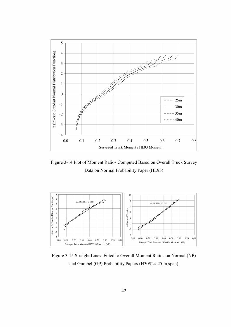
42
-4
-3
-2
-1
0
1
2
3
4
5
0.0 0.1 0.2 0.3 0.4 0.5 0.6 0.7 0.8
Surveyed Truck Moment / HL93 Moment
z (I
nver
se S
tand
art N
orm
al D
istr
ibut
ion
Fun
ctio
n)
.
25m
30m
35m
40m
Figure 3-14 Plot of Moment Ratios Computed Based on Overall Truck Survey
Data on Normal Probability Paper (HL93)
y = 10.808x - 2.3887
-4
-3
-2
-1
0
1
2
3
4
5
0.00 0.10 0.20 0.30 0.40 0.50 0.60 0.70 0.80
Surveyed Truck Moments / H30S24 Moments (NP)
z (I
nver
se O
f S
tand
ard
Nor
mal
Dis
trib
utio
n) .
y = 19.998x - 3.6112
-4
-2
0
2
4
6
8
10
0.00 0.10 0.20 0.30 0.40 0.50 0.60 0.70 0.80
Surveyed Truck Moments / H30S24 Moments (GP)
η (R
educ
ed V
aria
te)
.
Figure 3-15 Straight Lines Fitted to Overall Moment Ratios on Normal (NP)
and Gumbel (GP) Probability Papers (H30S24-25 m span)

43
y = 9.2526x - 2.3887
-4
-3
-2
-1
0
1
2
3
4
5
0.00 0.10 0.20 0.30 0.40 0.50 0.60 0.70 0.80
Surveyed Truck Moments / HL93 Moments (NP)
z (I
nver
se O
f S
tand
ard
Nor
mal
Dis
trib
utio
n) .
y = 17.12x - 3.6112
-4
-2
0
2
4
6
8
10
0.00 0.10 0.20 0.30 0.40 0.50 0.60 0.70 0.80
Surveyed Truck Moments / HL93 Moments (GP)
η (R
educ
ed V
aria
te)
.
Figure 3-16 Straight Lines Fitted to Overall Moment Ratios on Normal (NP)
and Gumbel (GP) Probability Papers (HL93-25 m span)
y = 11.374x - 2.5688
-4
-3
-2
-1
0
1
2
3
4
5
0.00 0.10 0.20 0.30 0.40 0.50 0.60 0.70 0.80
Surveyed Truck Moment / H30S24 Moments (NP)
z (I
nver
se O
f S
tand
ard
Nor
mal
Dis
trib
utio
n) .
y = 20.333x - 3.6093
-4
-2
0
2
4
6
8
10
0.00 0.10 0.20 0.30 0.40 0.50 0.60 0.70 0.80
Surveyed Truck Moment / H30S24 Moments (GP)
η (R
educ
ed V
aria
te)
.
Figure 3-17 Straight Lines Fitted to Overall Moment Ratios on Normal (NP)
and Gumbel (GP) Probability Papers (H30S24-30 m span)
y = 10.211x - 2.5688
-4
-3
-2
-1
0
1
2
3
4
5
0.00 0.10 0.20 0.30 0.40 0.50 0.60 0.70 0.80
Surveyed Truck Moment / HL93 Moments (NP)
z (I
nver
se O
f S
tand
ard
Nor
mal
Dis
trib
utio
n) .
y = 18.255x - 3.6093
-4
-2
0
2
4
6
8
10
0.00 0.10 0.20 0.30 0.40 0.50 0.60 0.70 0.80
Surveyed Truck Moment / HL93 Moments (GP)
η (R
educ
ed V
aria
te)
.
Figure 3-18 Straight Lines Fitted to Overall Moment Ratios on Normal (NP)
and Gumbel (GP) Probability Papers (HL93-30 m span)
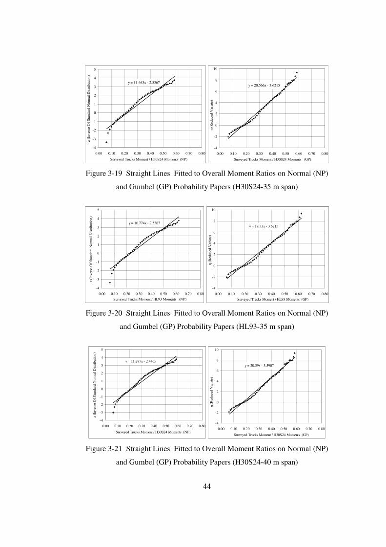
44
y = 11.463x - 2.5367
-4
-3
-2
-1
0
1
2
3
4
5
0.00 0.10 0.20 0.30 0.40 0.50 0.60 0.70 0.80
Surveyed Trucks Moment / H30S24 Moments (NP)
z (I
nver
se O
f S
tand
ard
Nor
mal
Dis
trib
utio
n) .
y = 20.566x - 3.6215
-4
-2
0
2
4
6
8
10
0.00 0.10 0.20 0.30 0.40 0.50 0.60 0.70 0.80
Surveyed Trucks Moment / H30S24 Moments (GP)
η (R
educ
ed V
aria
te)
.
Figure 3-19 Straight Lines Fitted to Overall Moment Ratios on Normal (NP)
and Gumbel (GP) Probability Papers (H30S24-35 m span)
y = 10.774x - 2.5367
-4
-3
-2
-1
0
1
2
3
4
5
0.00 0.10 0.20 0.30 0.40 0.50 0.60 0.70 0.80
Surveyed Trucks Moment / HL93 Moments (NP)
z (I
nver
se O
f S
tand
ard
Nor
mal
Dis
trib
utio
n) .
y = 19.33x - 3.6215
-4
-2
0
2
4
6
8
10
0.00 0.10 0.20 0.30 0.40 0.50 0.60 0.70 0.80
Surveyed Trucks Moment / HL93 Moments (GP)
η (R
educ
ed V
aria
te)
.
Figure 3-20 Straight Lines Fitted to Overall Moment Ratios on Normal (NP)
and Gumbel (GP) Probability Papers (HL93-35 m span)
y = 11.287x - 2.4465
-4
-3
-2
-1
0
1
2
3
4
5
0.00 0.10 0.20 0.30 0.40 0.50 0.60 0.70 0.80
Surveyed Trucks Moment / H30S24 Moments (NP)
z (I
nver
se O
f S
tand
ard
Nor
mal
Dis
trib
utio
n) .
y = 20.59x - 3.5907
-4
-2
0
2
4
6
8
10
0.00 0.10 0.20 0.30 0.40 0.50 0.60 0.70 0.80
Surveyed Trucks Moment / H30S24 Moments (GP)
η (R
educ
ed V
aria
te)
.
Figure 3-21 Straight Lines Fitted to Overall Moment Ratios on Normal (NP)
and Gumbel (GP) Probability Papers (H30S24-40 m span)

45
y = 11.087x - 2.4465
-4
-3
-2
-1
0
1
2
3
4
5
0.00 0.10 0.20 0.30 0.40 0.50 0.60 0.70 0.80
Surveyed Trucks Moment / HL93 Moments (NP)
z (I
nver
se O
f S
tand
ard
Nor
mal
Dis
trib
utio
n) .
y = 20.225x - 3.5907
-4
-2
0
2
4
6
8
10
0.00 0.10 0.20 0.30 0.40 0.50 0.60 0.70 0.80Surveyed Trucks Moment / HL93 Moments (GP)
η (R
educ
ed V
aria
te)
.
Figure 3-22 Straight Lines Fitted to Overall Moment Ratios on Normal (NP)
and Gumbel (GP) Probability Papers (HL93-40 m span)
y = 21.998x - 4.5023
-4
-2
0
2
4
6
8
10
0.00 0.10 0.20 0.30 0.40 0.50 0.60 0.70 0.80
Surveyed Truck Moments / H30S24 Moments (GP)
η (R
educ
ed V
aria
te)
.
y = 18.832x - 4.5023
-4
-2
0
2
4
6
8
10
0.00 0.10 0.20 0.30 0.40 0.50 0.60 0.70 0.80
Surveyed Truck Moments / HL93 Moments (GP)
η (R
educ
ed V
aria
te)
.
Figure 3-23 Straight Lines Fitted to the Upper Tail of Moment Ratios Plotted
on Gumbel (GP) Probability Papers (25 m span)
y = 22.385x - 4.5184
-4
-2
0
2
4
6
8
10
0.00 0.10 0.20 0.30 0.40 0.50 0.60 0.70 0.80
Surveyed Truck Moment / H30S24 Moments (GP)
η (R
educ
ed V
aria
te)
.
y = 20.096x - 4.5184
-4
-2
0
2
4
6
8
10
0.00 0.10 0.20 0.30 0.40 0.50 0.60 0.70 0.80
Surveyed Truck Moment / HL93 Moments (GP)
η (R
educ
ed V
aria
te)
.
Figure 3-24 Straight Lines Fitted to the Upper Tail of Moment Ratios Plotted
on Gumbel (GP) Probability Papers (30 m span)
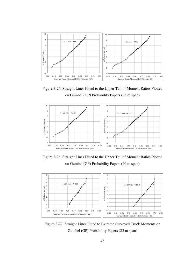
46
y = 22.816x - 4.603
-4
-2
0
2
4
6
8
10
0.00 0.10 0.20 0.30 0.40 0.50 0.60 0.70 0.80
Surveyed Trucks Moment / H30S24 Moments (GP)
η (R
educ
ed V
aria
te)
.y = 21.445x - 4.603
-4
-2
0
2
4
6
8
10
0.00 0.10 0.20 0.30 0.40 0.50 0.60 0.70 0.80
Surveyed Trucks Moment / HL93 Moments (GP)
η (R
educ
ed V
aria
te)
.
Figure 3-25 Straight Lines Fitted to the Upper Tail of Moment Ratios Plotted
on Gumbel (GP) Probability Papers (35 m span)
y = 22.462x - 4.3957
-4
-2
0
2
4
6
8
10
0.00 0.10 0.20 0.30 0.40 0.50 0.60 0.70 0.80
Surveyed Trucks Moment / H30S24 Moments (GP)
η (R
educ
ed V
aria
te)
.
y = 22.064x - 4.3957
-4
-2
0
2
4
6
8
10
0.00 0.10 0.20 0.30 0.40 0.50 0.60 0.70 0.80
Surveyed Trucks Moment / HL93 Moments (GP)
η (R
educ
ed V
aria
te)
.
Figure 3-26 Straight Lines Fitted to the Upper Tail of Moment Ratios Plotted
on Gumbel (GP) Probability Papers (40 m span)
y = 23.026x - 7.4019
-1
0
1
2
3
4
5
6
7
8
0.00 0.10 0.20 0.30 0.40 0.50 0.60 0.70 0.80
Surveyed Truck Moments / H30S24 Moments (GP)
η (R
educ
ed V
aria
te)
.
y = 19.712x - 7.4019
-1
0
1
2
3
4
5
6
7
8
0.00 0.10 0.20 0.30 0.40 0.50 0.60 0.70 0.80
Surveyed Truck Moments / HL93 Moments (GP)
η (R
educ
ed V
aria
te)
.
Figure 3-27 Straight Lines Fitted to Extreme Surveyed Truck Moments on
Gumbel (GP) Probability Papers (25 m span)
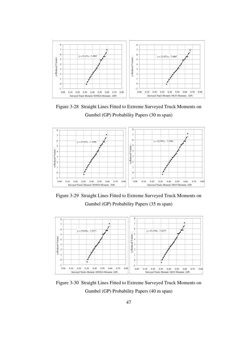
47
y = 23.47x - 7.4967
-1
0
1
2
3
4
5
6
7
8
0.00 0.10 0.20 0.30 0.40 0.50 0.60 0.70 0.80
Surveyed Truck Moment / H30S24 Moments (GP)
η (R
educ
ed V
aria
te)
.
y = 21.071x - 7.4967
-1
0
1
2
3
4
5
6
7
8
0.00 0.10 0.20 0.30 0.40 0.50 0.60 0.70 0.80
Surveyed Truck Moment / HL93 Moments (GP)
η (R
educ
ed V
aria
te)
.
Figure 3-28 Straight Lines Fitted to Extreme Surveyed Truck Moments on
Gumbel (GP) Probability Papers (30 m span)
y = 23.947x - 7.3296
-1
0
1
2
3
4
5
6
7
8
0.00 0.10 0.20 0.30 0.40 0.50 0.60 0.70 0.80
Surveyed Trucks Moment / H30S24 Moments (GP)
η (R
educ
ed V
aria
te)
.
y = 22.507x - 7.3296
-1
0
1
2
3
4
5
6
7
8
0.00 0.10 0.20 0.30 0.40 0.50 0.60 0.70 0.80
Surveyed Trucks Moment / HL93 Moments (GP)
η (R
educ
ed V
aria
te)
.
Figure 3-29 Straight Lines Fitted to Extreme Surveyed Truck Moments on
Gumbel (GP) Probability Papers (35 m span)
y = 23.659x - 7.2277
-1
0
1
2
3
4
5
6
7
8
0.00 0.10 0.20 0.30 0.40 0.50 0.60 0.70 0.80
Surveyed Trucks Moment / H30S24 Moments (GP)
η (R
educ
ed V
aria
te)
.
y = 23.239x - 7.2277
-1
0
1
2
3
4
5
6
7
8
0.00 0.10 0.20 0.30 0.40 0.50 0.60 0.70 0.80
Surveyed Trucks Moment / HL93 Moments (GP)
η (R
educ
ed V
aria
te)
.
Figure 3-30 Straight Lines Fitted to Extreme Surveyed Truck Moments on
Gumbel (GP) Probability Papers (40 m span)

48
3.3.3.2 Mean Maximum Moments Predicted by Extrapolation
In the current AASHTO LRFD bridge design specification, the return period of
maximum live load is taken as 75 years for live load equivalent to the design
life of bridges, 75 years. For this reason, the expected maximum live load
effect in a 75 year time period shall be determined. It is impossible to obtain
future truck survey data for this time period. Thus, that is done by extrapolating
the cumulative distribution functions to 75 years shown in Figures 3-15 to 3-
30.
Extrapolations are carried out based on the procedure and assumptions of
Nowak’s study on the calibration of AASHTO LRFD [3]. It is assumed that
truck survey data represents two weeks of heavy traffic on a bridge with
average daily traffic of 1000 trucks. The extend of the CDFs of moment ratios
shows the longer periods of time, e.g. 2 months, a year, 10 years, 50 years or
75 years. For example, there are 1950 two-week periods in 75 years. Therefore,
the total number of trucks for 75 years can be calculated by multiplying the
number of trucks corresponding to two-week time period, 1950, which is
1950x10000=20 million (10000 is the number of truck in two week time
period). Therefore, the probability of occurrence of the heaviest truck in this
population is 1/20000000 =5x10⁻⁸; this probability corresponds to z=5.33
( 33.5]105[ 81 =⋅ −−φ ) on the vertical axis of the plots on the normal probability
paper, η =16.81 ( 81.16]]105ln[ln[ 8 =⋅−− − ) on the vertical axis of the plots on
Gumbel probability paper. It has also been observed that the change in volume
of traffic computed based on this approach do not significantly change the
probability parameter used in the extrapolation methods. For instance, a two
times more truck traffic on bridge will result in (z= 45.5]105.2[ 81 =⋅ −−φ ) in a
75 year time period that is only a 2% [(5.45/5.33-1)x100] increase in the
probability parameter. Similar observations can also be made for the listed
values of the z parameter shown in Table 3-8.
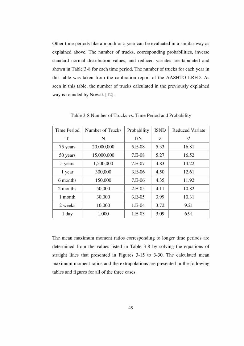
49
Other time periods like a month or a year can be evaluated in a similar way as
explained above. The number of trucks, corresponding probabilities, inverse
standard normal distribution values, and reduced variates are tabulated and
shown in Table 3-8 for each time period. The number of trucks for each year in
this table was taken from the calibration report of the AASHTO LRFD. As
seen in this table, the number of trucks calculated in the previously explained
way is rounded by Nowak [12].
Table 3-8 Number of Trucks vs. Time Period and Probability
Time Period Number of Trucks Probability ISND Reduced Variate
T N 1/N z η
75 years 20,000,000 5.E-08 5.33 16.81
50 years 15,000,000 7.E-08 5.27 16.52
5 years 1,500,000 7.E-07 4.83 14.22
1 year 300,000 3.E-06 4.50 12.61
6 months 150,000 7.E-06 4.35 11.92
2 months 50,000 2.E-05 4.11 10.82
1 month 30,000 3.E-05 3.99 10.31
2 weeks 10,000 1.E-04 3.72 9.21
1 day 1,000 1.E-03 3.09 6.91
The mean maximum moment ratios corresponding to longer time periods are
determined from the values listed in Table 3-8 by solving the equations of
straight lines that presented in Figures 3-15 to 3-30. The calculated mean
maximum moment ratios and the extrapolations are presented in the following
tables and figures for all of the three cases.

50
Table 3-9 Mean Maximum Moment Ratios for H30-S24 (Overall)
Surveyed Truck Moment / H30-S24 Moment Span (m) 1 day 2 weeks 1 month 2 months 6 months 1 year 5 years 50 years 75 years
25 0.53 0.64 0.70 0.72 0.78 0.81 0.89 1.01 1.02
30 0.52 0.63 0.68 0.71 0.76 0.80 0.88 0.99 1.00
35 0.51 0.62 0.68 0.70 0.76 0.79 0.87 0.98 0.99
40 0.51 0.62 0.68 0.70 0.75 0.79 0.87 0.98 0.99
Table 3-10 Mean Maximum Moment Ratios for HL-93 (Overall)
Surveyed Truck Moment / HL-93 Moment Span (m) 1 day 2 weeks 1 month 2 months 6 months 1 year 5 years 50 years 75 years
25 0.61 0.75 0.81 0.84 0.91 0.95 1.04 1.18 1.19
30 0.58 0.70 0.76 0.79 0.85 0.89 0.98 1.10 1.12
35 0.54 0.66 0.72 0.75 0.80 0.84 0.92 1.04 1.06
40 0.52 0.63 0.69 0.71 0.77 0.80 0.88 0.99 1.01
Table 3-11 Mean Maximum Moment Ratios for H30-S24 (Upper Tail)
Surveyed Truck Moment / H30-S24 Moment Span (m) 1 day 2 weeks 1 month 2 months 6 months 1 year 5 years 50 years 75 years
25 0.52 0.62 0.67 0.70 0.75 0.78 0.85 0.96 0.97
30 0.51 0.61 0.66 0.69 0.73 0.77 0.84 0.94 0.95
35 0.50 0.61 0.65 0.68 0.72 0.75 0.83 0.93 0.94
40 0.50 0.61 0.65 0.68 0.73 0.76 0.83 0.93 0.94

51
Table 3-12 Mean Maximum Moment Ratios for HL-93 (Upper Tail)
Surveyed Truck Moment / HL-93 Moment Span (m) 1 day 2 weeks 1 month 2 months 6 months 1 year 5 years 50 years 75 years
25 0.61 0.73 0.79 0.81 0.87 0.91 0.99 1.12 1.13
30 0.57 0.68 0.74 0.76 0.82 0.85 0.93 1.05 1.06
35 0.54 0.64 0.70 0.72 0.77 0.80 0.88 0.99 1.00
40 0.51 0.62 0.67 0.69 0.74 0.77 0.84 0.95 0.96
Table 3-13 Mean Maximum Moment Ratios for H30-S24 (Extreme)
Surveyed Truck Moment / H30-S24 Moment Span (m) 1 day 2 weeks 1 month 2 months 6 months 1 year 5 years 50 years 75 years
25 0.62 0.72 0.77 0.79 0.84 0.87 0.94 1.04 1.05
30 0.61 0.71 0.76 0.78 0.83 0.86 0.93 1.02 1.04
35 0.59 0.69 0.74 0.76 0.80 0.83 0.90 1.00 1.01
40 0.60 0.69 0.74 0.76 0.81 0.84 0.91 1.00 1.02
Table 3-14 Mean Maximum Moment Ratios for HL-93 (Extreme)
Surveyed Truck Moment / HL-93 Moment Span (m) 1 day 2 weeks 1 month 2 months 6 months 1 year 5 years 50 years 75 years
25 0.73 0.84 0.90 0.92 0.98 1.02 1.10 1.21 1.23
30 0.68 0.79 0.85 0.87 0.92 0.95 1.03 1.14 1.15
35 0.63 0.73 0.78 0.81 0.86 0.89 0.96 1.06 1.07
40 0.61 0.71 0.75 0.78 0.82 0.85 0.92 1.02 1.03
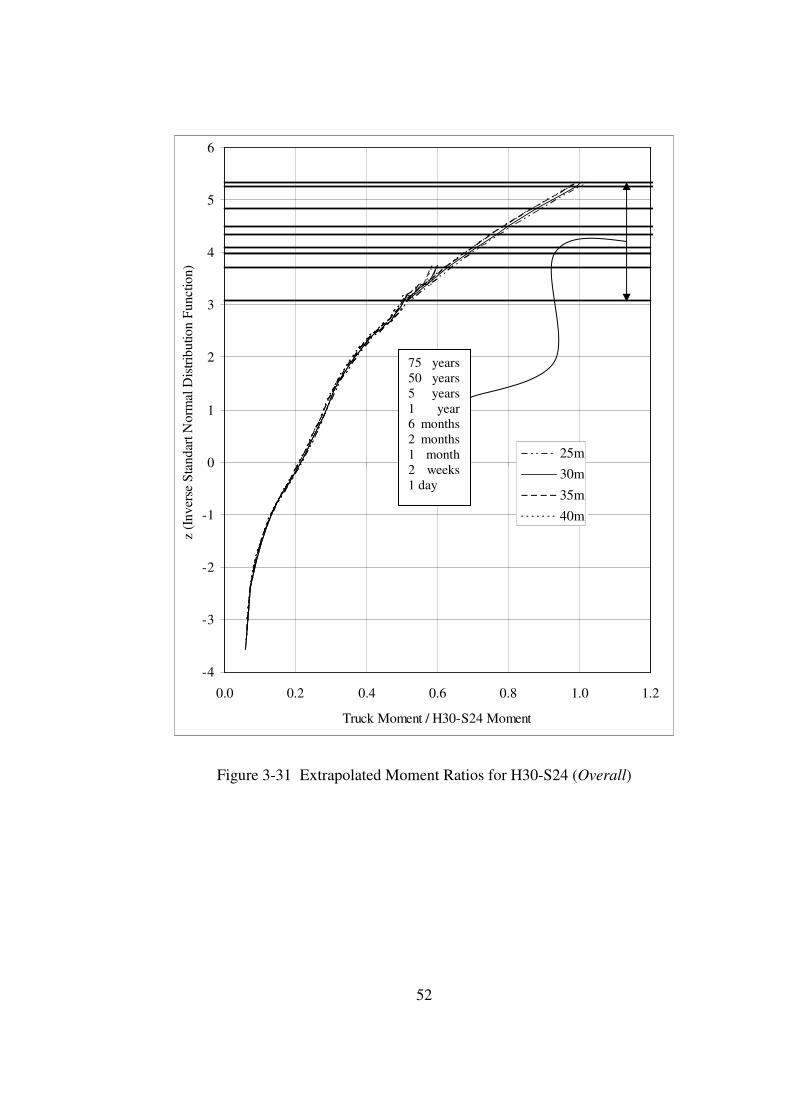
52
-4
-3
-2
-1
0
1
2
3
4
5
6
0.0 0.2 0.4 0.6 0.8 1.0 1.2
Truck Moment / H30-S24 Moment
z (I
nver
se S
tand
art N
orm
al D
istr
ibut
ion
Fun
ctio
n)
.
25m
30m
35m
40m
Figure 3-31 Extrapolated Moment Ratios for H30-S24 (Overall)
75 years 50 years 5 years 1 year 6 months 2 months 1 month 2 weeks 1 day
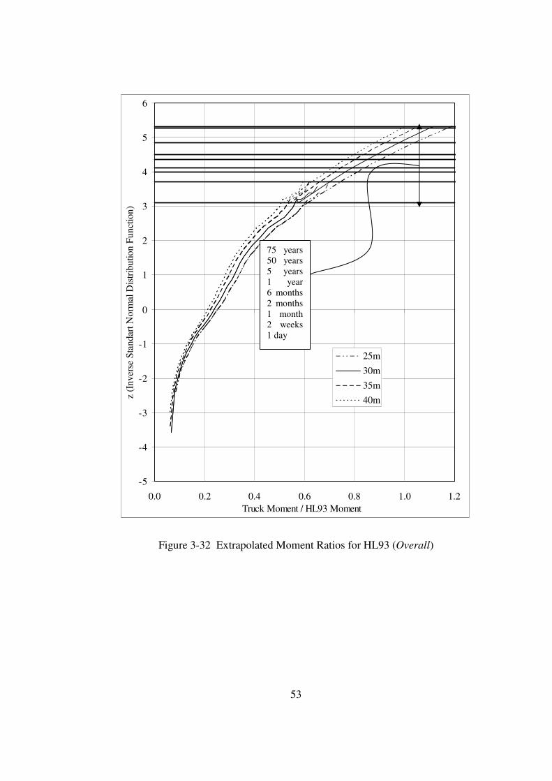
53
-5
-4
-3
-2
-1
0
1
2
3
4
5
6
0.0 0.2 0.4 0.6 0.8 1.0 1.2Truck Moment / HL93 Moment
z (I
nver
se S
tand
art N
orm
al D
istr
ibut
ion
Fun
ctio
n)
...
25m
30m
35m
40m
Figure 3-32 Extrapolated Moment Ratios for HL93 (Overall)
75 years 50 years 5 years 1 year 6 months 2 months 1 month 2 weeks 1 day

54
-4
-3
-2
-1
0
1
2
3
4
5
6
0.0 0.2 0.4 0.6 0.8 1.0 1.2
Truck Moment / H30-S24 Moment
z (I
nver
se S
tand
art N
orm
al D
istr
ibut
ion
Fun
ctio
n)
.
25m
30m
35m
40m
Figure 3-33 Extrapolated Moment Ratios for H30-S24 (Upper Tail)
75 years 50 years 5 years 1 year 6 months 2 months 1 month 2 weeks 1 day
55
-5
-4
-3
-2
-1
0
1
2
3
4
5
6
0.0 0.2 0.4 0.6 0.8 1.0 1.2Truck Moment / HL93 Moment
z (I
nver
se S
tand
art N
orm
al D
istr
ibut
ion
Fun
ctio
n)
...
25m
30m
35m
40m
Figure 3-34 Extrapolated Moment Ratios for HL93 (Upper Tail)
75 years 50 years 5 years 1 year 6 months 2 months 1 month 2 weeks 1 day
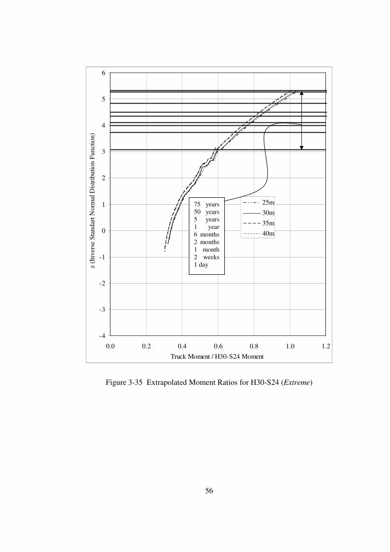
56
-4
-3
-2
-1
0
1
2
3
4
5
6
0.0 0.2 0.4 0.6 0.8 1.0 1.2
Truck Moment / H30-S24 Moment
z (I
nver
se S
tand
art N
orm
al D
istr
ibut
ion
Fun
ctio
n)
.
25m
30m
35m
40m
Figure 3-35 Extrapolated Moment Ratios for H30-S24 (Extreme)
75 years 50 years 5 years 1 year 6 months 2 months 1 month 2 weeks 1 day
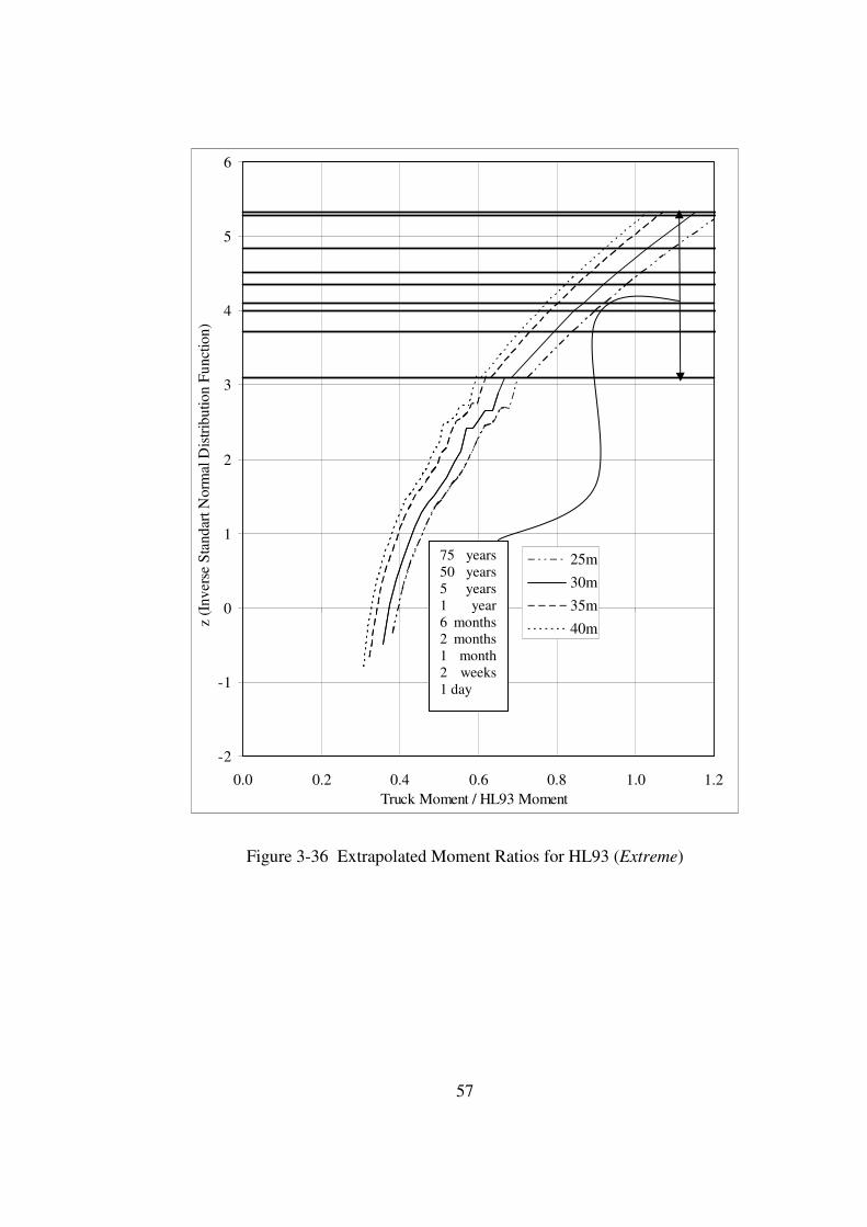
57
-2
-1
0
1
2
3
4
5
6
0.0 0.2 0.4 0.6 0.8 1.0 1.2Truck Moment / HL93 Moment
z (I
nver
se S
tand
art N
orm
al D
istr
ibut
ion
Fun
ctio
n)
...
25m
30m
35m
40m
Figure 3-36 Extrapolated Moment Ratios for HL93 (Extreme)
75 years 50 years 5 years 1 year 6 months 2 months 1 month 2 weeks 1 day

58
3.3.3.3 Estimation of the Coefficient of Variation
The coefficients of variation for each of the three cases are calculated based on
the data and by fitting straight lines to the data points plotted on Gumbel
probability paper. Firstly, according to the basic statistical concepts, the
coefficients of variation were estimated by using all calculated surveyed truck
moment ratios by the following expressions:
N
Mi∑=µ and
( )1
22
−
−∑=
N
Mi µσ ⇒
µ
σ=COV (3-5)
where, µ is the mean value, σ is the standard deviation, COV is the coefficient
of variation, Mi is the ith moment ratio , N is the total number of data.
Calculated coefficients of variation are presented in Table 3-15. Due to the
same truck survey data, the coefficient of variation is the same for each
investigated case.
Table 3-15 Mean, Standard Deviation and Coefficient of Variation Values
Computed from the Whole Data for each Span
Surveyed Truck M./H30-S24 M. Surveyed Truck M. / HL-93 M. Span Length
(m) max min µ σ COV max min µ σ COV
25 0.595 0.055 0.216 0.075 0.348 0.695 0.065 0.253 0.088 0.348
30 0.587 0.055 0.213 0.074 0.348 0.654 0.061 0.238 0.083 0.348
35 0.582 0.054 0.211 0.073 0.347 0.619 0.058 0.225 0.078 0.347
40 0.578 0.054 0.209 0.073 0.347 0.588 0.055 0.213 0.074 0.347

59
For Gumbel distribution, the coefficient of variation of live load is estimated
from the straight lines fitted to the data points. The cumulative distribution
function of the Gumbel distribution for maxima is given by [15]
∞<<∞−
−−−== x
xxFy ;expexp),;(
δ
λδλ (3-6)
where, λ and δ are the Gumbel distribution parameters. Then, the straight line
equation that was fitted to the plotted points on Gumbel probability paper
becomes [15]
( )δ
ληη
−=→
−==
x
yyh
1loglog (3-7)
The two parameters λ and δ can be estimated by setting 0=η and 1=η , [15]
λλ =→−= xx0 and δλδ
λ+=→
−= x
x1 (3-8)
After fitting the straight line on Gumbel probability paper, the abscissas
associated with ordinate values 0 and 1 of the reduced variate,η , give the
values of λ and δλ + , respectively . After obtaining the values of λ andδ , the
mean and variance of the Gumbel distribution can be calculated by the
following expressions [15]:
δλµ 5772.0+= and 6
222 δπ
σ = (3-9)
where, µ and σ are the mean and standard variation, respectively.
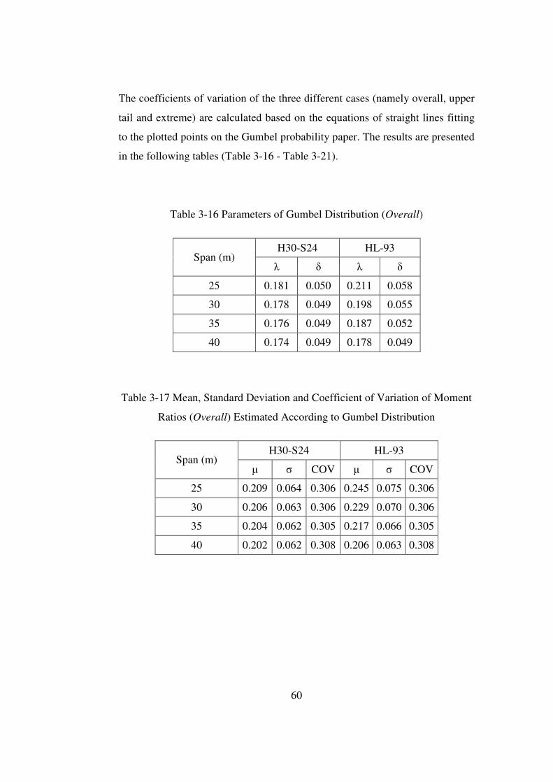
60
The coefficients of variation of the three different cases (namely overall, upper
tail and extreme) are calculated based on the equations of straight lines fitting
to the plotted points on the Gumbel probability paper. The results are presented
in the following tables (Table 3-16 - Table 3-21).
Table 3-16 Parameters of Gumbel Distribution (Overall)
H30-S24 HL-93 Span (m)
λ δ λ δ
25 0.181 0.050 0.211 0.058
30 0.178 0.049 0.198 0.055
35 0.176 0.049 0.187 0.052
40 0.174 0.049 0.178 0.049
Table 3-17 Mean, Standard Deviation and Coefficient of Variation of Moment
Ratios (Overall) Estimated According to Gumbel Distribution
H30-S24 HL-93 Span (m)
µ σ COV µ σ COV
25 0.209 0.064 0.306 0.245 0.075 0.306
30 0.206 0.063 0.306 0.229 0.070 0.306
35 0.204 0.062 0.305 0.217 0.066 0.305
40 0.202 0.062 0.308 0.206 0.063 0.308

61
Table 3-18 Parameters of Gumbel Distribution (Upper Tail)
H30-S24 HL-93 Span (m)
λ δ λ δ
25 0.205 0.0455 0.239 0.053
30 0.202 0.0447 0.225 0.05
35 0.202 0.0438 0.215 0.047
40 0.196 0.0445 0.199 0.045
Table 3-19 Mean, Standard Deviation and Coefficient of Variation of Moment
Ratios (Upper Tail) Estimated According to Gumbel Distribution
H30-S24 HL-93 Span (m)
µ σ COV µ σ COV
25 0.231 0.058 0.252 0.270 0.068 0.252
30 0.228 0.057 0.252 0.254 0.064 0.252
35 0.227 0.056 0.248 0.242 0.060 0.248
40 0.221 0.057 0.258 0.225 0.058 0.258
Table 3-20 Parameters of Gumbel Distribution (Extreme)
H30-S24 HL-93 Span (m)
λ δ λ δ
25 0.321 0.0434 0.376 0.051
30 0.319 0.0426 0.356 0.047
35 0.306 0.0418 0.326 0.044
40 0.305 0.0423 0.311 0.043

62
Table 3-21 Mean, Standard Deviation and Coefficient of Variation of Moment
Ratios (Extreme) Estimated According to Gumbel Distribution
H30-S24 HL-93 Span (m)
µ σ COV µ σ COV
25 0.347 0.056 0.161 0.405 0.065 0.161
30 0.344 0.055 0.159 0.383 0.061 0.159
35 0.330 0.054 0.162 0.351 0.057 0.162
40 0.330 0.054 0.164 0.336 0.055 0.164
3.3.3.4 Comparison of the Different Extrapolation Cases
The mean maximum moments and coefficients of variation are calculated for
three cases: overall original surveyed truck moments, upper tail (90 percentile
and greater) of overall surveyed truck moments, and extreme surveyed truck
moments. Calculations are carried out for both H30S24 and HL93 design truck
loadings. The 75-year maximum mean moment ratios are plotted for H30S24
and HL93 loadings in Figure 3-37 and Figure 3-38, respectively, and
coefficients of variation are shown in Figure 3-39. As the figures indicate, the
mean moment ratios are higher and coefficient of variation is considerably
lower for the case that the extrapolation is done from straight lines fitting to
extreme surveyed truck moments. Extrapolation done by overall surveyed truck
moments results in high coefficient of variation due to the fact that both
maximum and minimum load effects are included. However, in reliability
assessment, the load should be considered to be maximum to estimate the
minimum safety level of design. Therefore, in this study, the statistical
parameters of live load estimated by the extreme surveyed truck moment ratios
are taken.

63
0.7
0.8
0.9
1
1.1
1.2
1.3
25 30 35 40
Span Length (m)
75 Y
ear
Mea
n M
ax.
Mom
ent R
atio
.Overall
Upper Tail
Extreme
Figure 3-37 Variation of 75 year Mean Maximum Moment Ratio with Span
Lengths According to Different Assumptions on Extrapolation of Data for
H30S24
0.7
0.8
0.9
1
1.1
1.2
1.3
25 30 35 40Span Length (m)
75 Y
ear
Mea
n M
ax. M
omen
t Rat
io .
Overall
Upper Tail
Extreme
Figure 3-38 Variation of 75 year Mean Maximum Moment Ratio with Span
Lengths According to Different Assumptions on Extrapolation of Data for
HL93
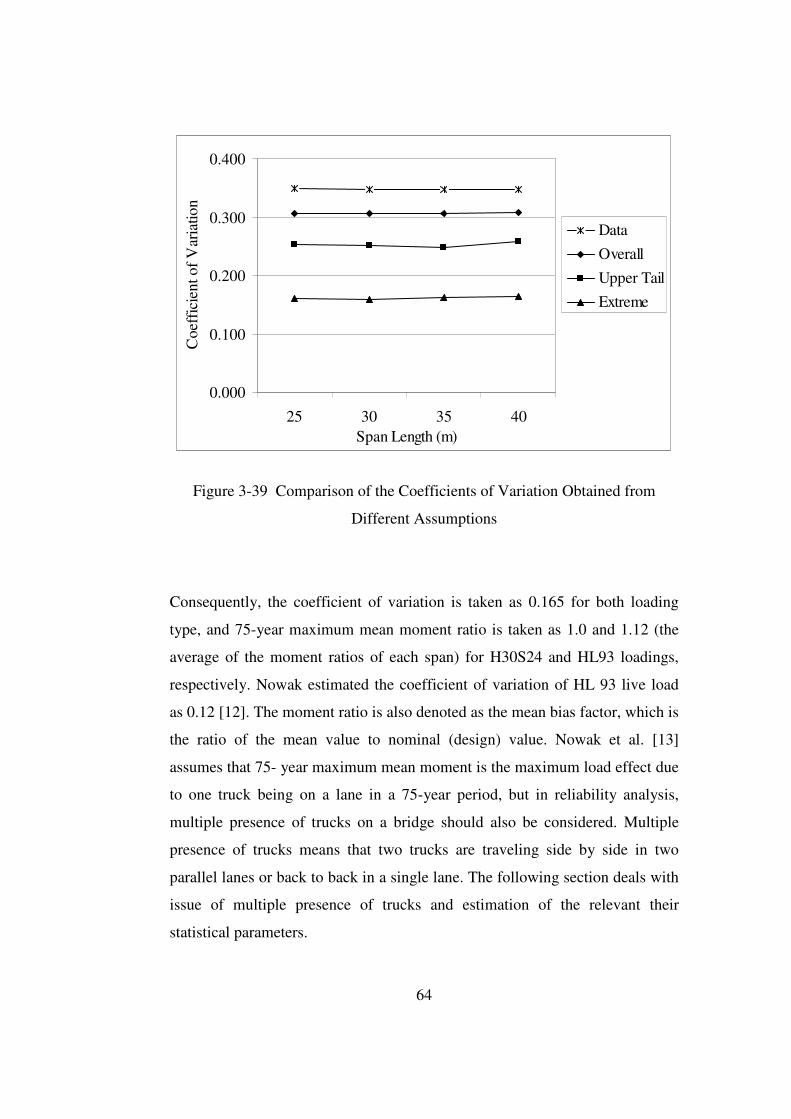
64
0.000
0.100
0.200
0.300
0.400
25 30 35 40Span Length (m)
Coe
ffic
ient
of
Var
iatio
n .
Data
Overall
Upper Tail
Extreme
Figure 3-39 Comparison of the Coefficients of Variation Obtained from
Different Assumptions
Consequently, the coefficient of variation is taken as 0.165 for both loading
type, and 75-year maximum mean moment ratio is taken as 1.0 and 1.12 (the
average of the moment ratios of each span) for H30S24 and HL93 loadings,
respectively. Nowak estimated the coefficient of variation of HL 93 live load
as 0.12 [12]. The moment ratio is also denoted as the mean bias factor, which is
the ratio of the mean value to nominal (design) value. Nowak et al. [13]
assumes that 75- year maximum mean moment is the maximum load effect due
to one truck being on a lane in a 75-year period, but in reliability analysis,
multiple presence of trucks on a bridge should also be considered. Multiple
presence of trucks means that two trucks are traveling side by side in two
parallel lanes or back to back in a single lane. The following section deals with
issue of multiple presence of trucks and estimation of the relevant their
statistical parameters.
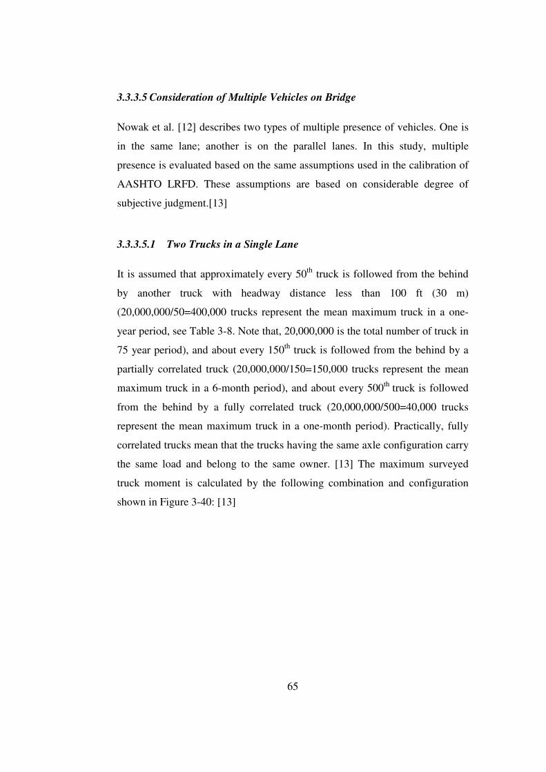
65
3.3.3.5 Consideration of Multiple Vehicles on Bridge
Nowak et al. [12] describes two types of multiple presence of vehicles. One is
in the same lane; another is on the parallel lanes. In this study, multiple
presence is evaluated based on the same assumptions used in the calibration of
AASHTO LRFD. These assumptions are based on considerable degree of
subjective judgment.[13]
3.3.3.5.1 Two Trucks in a Single Lane
It is assumed that approximately every 50th truck is followed from the behind
by another truck with headway distance less than 100 ft (30 m)
(20,000,000/50=400,000 trucks represent the mean maximum truck in a one-
year period, see Table 3-8. Note that, 20,000,000 is the total number of truck in
75 year period), and about every 150th truck is followed from the behind by a
partially correlated truck (20,000,000/150=150,000 trucks represent the mean
maximum truck in a 6-month period), and about every 500th truck is followed
from the behind by a fully correlated truck (20,000,000/500=40,000 trucks
represent the mean maximum truck in a one-month period). Practically, fully
correlated trucks mean that the trucks having the same axle configuration carry
the same load and belong to the same owner. [13] The maximum surveyed
truck moment is calculated by the following combination and configuration
shown in Figure 3-40: [13]

66
Figure 3-40 Sketch of Two Truck in Single Lane
a) Maximum 75 year Truck (Only one Truck)
b) Maximum 1 year truck (Truck 1) and average truck from survey (Truck
2),
c) Maximum 6 month truck (Truck 1) and maximum 1 day truck (Truck
2),
d) Maximum 1 month truck (Truck 1) and maximum 1 month truck
(Truck 2).
The minimum headway distance is assumed to be 50 ft (15 m), which is
conservative considering the braking distance [13]. Conservatively, in
calculating the moment values for two trucks in one lane, the minimum
distance headway is assumed to be the distance between load centers of two
trucks. The moment ratios are calculated for these truck combinations, and
presented in Table 3-22 and Table 3-23. As the results indicate, 75-year mean
maximum moments govern for all cases. The one-lane maximum mean
moment ratios are taken as 1.00 and 1.12 for H30S24 and HL93 loadings,
respectively. Note that, these values are the average of the moment ratios.
Headway Distance
Truck 1 Truck 2

67
Nowak et al. [12] estimated one-lane maximum mean moment ratio as between
1.23 and 1.36 for HL93.
Table 3-22 Maximum One Lane Truck Moment for H30S24 Loading
One Truck
Two Trucks Span (m) max 75
years max 1 year and average
max 6 months and max 1 day
two max 1 month
Max One Lane Span Moment
25 1.05 0.800 0.715 0.719 1.05
30 1.04 0.857 0.827 0.759 1.04
35 1.01 0.880 0.889 0.842 1.01
40 1.02 0.921 0.959 0.927 1.02
Table 3-23 Maximum One Lane Truck Moment for HL93 Loading
One Truck
Two Trucks Span (m) max 75
years max 1 year and average
max 6 months and max 1 day
two max 1 month
Max One Lane Span Moment
25 1.23 0.934 0.835 0.719 1.23
30 1.15 0.954 0.921 0.845 1.15
35 1.07 0.936 0.946 0.896 1.07
40 1.03 0.938 0.976 0.943 1.03
3.3.3.5.2 Trucks in Two Parallel Lanes
For two traffic lanes in the same direction, it is assumed that about every 15th
truck is travelling on the bridge simultaneously with another truck in the
adjacent lane and about every 150th truck with another truck that is partially
correlated, and about every 450th truck is fully correlated. Therefore, the
following combinations are considered: [13]

68
a) Maximum 75 year truck
b) Maximum 5 year truck and average truck from survey,
c) Maximum 6 month truck and maximum 1 day truck,
d) Maximum 2 month truck and maximum 2 month truck.
Nowak et al. [12] indicates that the side by side truck case equivalent to a two
month truck pass in the design life of a bridge is governing the load case
according to the results of simulations. In simulations, the trucks are placed 1.2
m (4 ft) apart. So, in this study, extrapolated two month truck moment ratios
are assumed for the case of multiple presence of trucks in two parallel lanes.
As indicated in Table 3-13 and Table 3-14, the two lane maximum mean
moment ratios are taken as 0.78 and 0.86 (average of moment ratios) for
H30S24 and HL93 loadings, respectively. Nowak et al. [12] estimated two-lane
maximum mean moment ratio to lie between 1.08 and 1.15 for HL93.
3.4 DYNAMIC LOAD ALLOWANCE
The static effect of design truck or tandem is increased by the percentage
specified in Table 3-24. In strength I and Service III Limit states, the dynamic
load allowance factor (impact factor, IM) is taken as %33. This factor is not
applied to lane load.
Table 3-24 Dynamic Load Allowance, IM (AASHTO LRFD Table 3.6.2.1-1)
Component IM
Deck Joints – All Limit States %75
All Other Component
-Fatigue and Fracture Limit State %15
-All Other Limit States %33

69
Hwang and Nowak et al. [16] aimed to develop a procedure to calculate the
dynamic load and to determine statistical parameters of the dynamic load to be
used in the development of a reliability-based bridge design code. The study
was carried out for different models developed for trucks, road surface
(roughness), and the bridges.
Figure 3-41 Maximum Static and Dynamic Deflections [16]
The dynamic load effect in a bridge is assessed in terms of the maximum static
( staD ) and dynamic deflections ( dynD ), as shown in Figure 3-41. The dynamic
load factor is expressed as the maximum dynamic deflection divided by the
maximum static deflection at mid-span. According to the research, the
following results were obtained: [16]
• The dynamic load factor decreases as the gross vehicle weight
increases.
• The dynamic and static live loads can be considered uncorrelated
except for 30 m span bridges (low degree of correlation was observed).
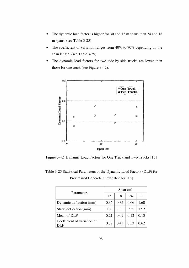
70
• The dynamic load factor is higher for 30 and 12 m spans than 24 and 18
m spans. (see Table 3-25)
• The coefficient of variation ranges from 40% to 70% depending on the
span length. (see Table 3-25)
• The dynamic load factors for two side-by-side trucks are lower than
those for one truck (see Figure 3-42).
Figure 3-42 Dynamic Load Factors for One Truck and Two Trucks [16]
Table 3-25 Statistical Parameters of the Dynamic Load Factors (DLF) for
Prestressed Concrete Girder Bridges [16]
Span (m) Parameters
12 18 24 30
Dynamic deflection (mm) 0.36 0.35 0.66 1.60
Static deflection (mm) 1.7 3.8 5.5 12.2
Mean of DLF 0.21 0.09 0.12 0.13
Coefficient of variation of DLF
0.72 0.43 0.53 0.62
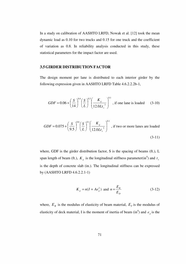
71
In a study on calibration of AASHTO LRFD, Nowak et al. [12] took the mean
dynamic load as 0.10 for two trucks and 0.15 for one truck and the coefficient
of variation as 0.8. In reliability analysis conducted in this study, these
statistical parameters for the impact factor are used.
3.5 GIRDER DISTRIBUTION FACTOR
The design moment per lane is distributed to each interior girder by the
following expression given in AASHTO LRFD Table 4.6.2.2.2b-1,
1.0
3
3.04.0
0.121406.0
+=
s
g
Lt
K
L
SSGDF , if one lane is loaded (3-10)
1.0
3
1.06.0
0.125.9075.0
+=
s
g
Lt
K
L
SSGDF , if two or more lanes are loaded
(3-11)
where, GDF is the girder distribution factor, S is the spacing of beams (ft.), L
span length of beam (ft.), gK is the longitudinal stiffness parameter(in4) and st
is the depth of concrete slab (in.). The longitudinal stiffness can be expressed
by (AASHTO LRFD 4.6.2.2.1-1)
)( 2gg AeInK += and
D
B
E
En = (3-12)
where, BE is the modulus of elasticity of beam material, FE is the modulus of
elasticity of deck material, I is the moment of inertia of beam (in4) and ge is the

72
distance between the centers of gravity of the basic beam and deck (in.). Note
that, n is a non-dimensional coefficient.
In the calibrations of AASHTO LRFD by Nowak [13], the bias factor for
girder distribution function is taken as 1.0 and coefficient of variation as 0.12.
In this research work, GDF calculated according to AASHTO LRFD results in
conservative values. In another research which compares the design codes,
Spanish Norma, Eurocode, and AASHTO LRFD [3], the bias factor and
coefficient of variation of GDF are taken as 0.93 and 0.12, respectively, and
these statistical parameters of GDF are also used in this study.
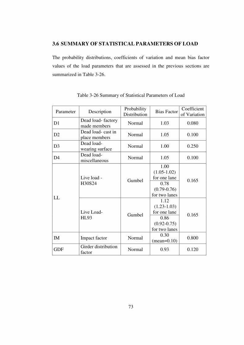
73
3.6 SUMMARY OF STATISTICAL PARAMETERS OF LOAD
The probability distributions, coefficients of variation and mean bias factor
values of the load parameters that are assessed in the previous sections are
summarized in Table 3-26.
Table 3-26 Summary of Statistical Parameters of Load
Parameter Description Probability Distribution
Bias Factor Coefficient of Variation
D1 Dead load- factory made members
Normal 1.03 0.080
D2 Dead load- cast in place members
Normal 1.05 0.100
D3 Dead load- wearing surface
Normal 1.00 0.250
D4 Dead load- miscellaneous
Normal 1.05 0.100
1.00 (1.05-1.02) for one lane Live load -
H30S24 Gumbel
0.78 (0.79-0.76) for two lanes
0.165
1.12 (1.23-1.03) for one lane
LL
Live Load- HL93
Gumbel 0.86
(0.92-0.75) for two lanes
0.165
IM Impact factor Normal 0.30
(mean=0.10) 0.800
GDF Girder distribution factor
Normal 0.93 0.120
74
CHAPTER 4
STATISTICS OF RESISTANCE
In reliability analysis, precast prestressed concrete girders are designed to
express nominal values of resistance parameters for both strength and service
limit states. The following chapter introduces design expressions and
procedures according to AASHTO LRFD bridge design specification [1]. In
addition, the statistical parameters of resistance that are required to calculate
the reliability index are assessed by the available local statistical data, as well
as relevant results reported by other studies are also presented.
4.1 NOMINAL FLEXURAL RESISTANCE CAPACITY
ACCORDING TO AASHTO LRFD DESIGN SPECIFICATION
The AASHTO LRFD Design Specifications introduce unified design
provisions, which are applicable to a variety of structures including concrete
members that are reinforced with a combination of rebars and prestressing
strands. These are called partially prestressed members. The design equations
can also be applicable when reinforcement bars or prestressing strands are not
present. [4]
Nominal flexural resistance capacity equations can be found in AASHTO
LRFD 5.7.3.1.1. [1] for bonded tendons. In prestressed concrete girders, the
tendon, which is a strand or a group of strands, is fully bonded to concrete. If
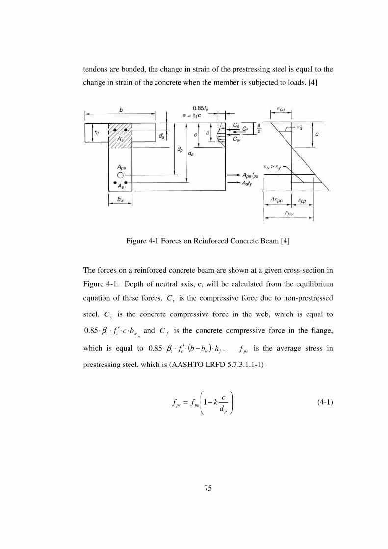
75
tendons are bonded, the change in strain of the prestressing steel is equal to the
change in strain of the concrete when the member is subjected to loads. [4]
Figure 4-1 Forces on Reinforced Concrete Beam [4]
The forces on a reinforced concrete beam are shown at a given cross-section in
Figure 4-1. Depth of neutral axis, c, will be calculated from the equilibrium
equation of these forces. sC is the compressive force due to non-prestressed
steel. wC is the concrete compressive force in the web, which is equal to
wc bcf ⋅⋅′⋅⋅ 185.0 β , and fC is the concrete compressive force in the flange,
which is equal to ( ) fwc hbbf ⋅−⋅′⋅⋅ 185.0 β . psf is the average stress in
prestressing steel, which is (AASHTO LRFD 5.7.3.1.1-1)
−=
p
pupsd
ckff 1 (4-1)

76
where, puf is the specified tensile strength of prestressing steel, bd is the
distance from extreme compression fiber to the centroid of the prestressing
strands, k is equal to (AASHTO LRFD 5.7.3.1.1-2)
−=
pu
py
f
fk 04.12 (4-2)
for low relaxation strands k is taken as 0.28 (AASHTO LRFD Table
C5.7.3.1.1-1).
The equilibrium equation can be expressed as nn CT =
ss
p
pupsn fAd
ckfAT +−= )1( (4-3)
ssfwcwcn fAhbbfcbfC ′′+−′+′= )(85.085.0 11 ββ (4-4)
Solving the equilibrium equation for c by utilizing Equation 4-3 and 4-4 will
yield to the following: (AASHTO LRFD 5.7.3.1.1-3),
dp
fkAbf
hbbffAfAfAc
pu
psc
fwcsssspups
+′
−−′′−+=
185.0
)(85.0
β
(4-5)
where, psA is the area of prestressing steel, sA is the area of mild steel tension
reinforcement, sA′ is area of compression reinforcement, cf ′ is the compressive
stress of deck concrete, sf is the yield strength of tension reinforcement, sf ′ is
stress in mild steel compression reinforcement at nominal flexural resistance,b
77
is the width of compression flange, wb is the width of web, fh is the depth of
compression flange, 1β is the stress factor of compression block (AASHTO
LRFD 5.7.2.2), which is expressed as follows:
>′≥−′−
≤′
MPafforMpaMpaf
aMPffor
cc
c
2865.07/)28(05.085.0
2828.0:1β (4-6)
Equation 4.5 is developed for T section compression block. For rectangular
compression block, b is equal to wb . Therefore, c becomes (AASHTO LRFD
5.7.3.1.1-4),
dp
fkAbf
fAfAfAc
pu
psc
sssspups
+′
′′−+=
185.0 β
(4-7)
The nominal moment capacity, nM , can be calculated at wC application point
(AASHTO LRFD 5.7.3.2.2-1)
)22
()(85.0
)2
()2
()2
(
f
fwc
ssssssppspsn
hahbbf
adfA
adfA
adfAM
−−′+
−′′′−−+−=
(4-8)
where, sd : distance from extreme compression fiber to the centroid of non
prestressed tensile reinforcement, sd ′ : distance from extreme compression fiber
to the centroid of non prestressed compression reinforcement, a: c1β ,depth of
equivalent stress block.

78
Under the circumstances of a rectangular section behavior and no compression
reinforcement or mild tension reinforcement, the flexural nominal moment
capacity can be computed from the equation given below
)2
(a
dfAM ppspsn −= (4-9)
4.2 TENSILE STRESS CHECK ACCORDING TO SERVICE III
LIMIT STATE
The required number of strands is usually estimated by limiting concrete
tensile stresses at the bottom fiber using Service III requirements of AASHTO
LRFD design specifications (see Section 3.1). It is due to the need to control
the cracking of concrete under 80% of service loads. Bottom fiber tensile stress
estimated for the load combination of Service III can be computed from basics
of elastic stress theory.
bc
LLLTwsb
b
sg
b
cpepe
bS
MMMM
S
MM
S
eP
A
Pf
)(8.0 +++−
+−+= (4-10)
where, bf is the bottom fiber tensile stress, gM is the unfactored bending
moment due to beam self-weight, sM is the unfactored bending moment due to
slab and haunch weights, wsM is the unfactored bending moment due to barrier
weights, LTM is the unfactored bending moment due to truck load, LLM is the
unfactored bending moment due to lane load, bS is the section modulus for the
extreme bottom fiber of the non-composite precast beam, bcS is the composite
section modulus for the extreme bottom fiber of the non-composite precast
beam, peP is the total prestressing force, and ce is the strand eccentricity.

79
The tensile stress in the bottom fiber of beam, bf ,should be smaller in
magnitude than the concrete limiting tensile stress, of either cf ′50.0
representing not worse than moderate corrosion conditions or
cf ′25.0 representing severe corrosive conditions (AASHTO LRFD Table
5.9.4.2.2-1). In this relationship, cf ′ is the specified 28-day concrete strength of
precast beam (MPa).
The total prestressing force, peP , is estimated by subtracting the prestressing
losses from the tensile stress capacity and multiplying it with the number of
prestressing steels. Total prestress loss (AASHTO LRFD 5.9.5.1-1) can be
computed from the equation below:
pLTpESpT fff ∆+∆=∆ (4-11)
where, pESf∆ is the sum of all losses or gains due to elastic shortening or
extension at the time of application of prestress, pLTf∆ describes the losses due
to long term shrinkage and creep of concrete, and relaxation of the steel.
The change in prestressing steel stress due to the elastic deformations of the
section may occur at any stage of loading. The loss due to elastic shortening
can be computed from the following relationship (AASHTO LRFD 5.9.5.2.3a-
1)
cgp
ct
p
pES fE
Ef =∆ (4-12)
80
where, cgpf is the concrete stress at the center of gravity of prestressing tendons
due to the prestressing force immediately after transfer and the self-weight of
the member at the section of maximum moment, and pE is the modulus of
elasticity of prestressing steel, and ctE is the modulus of elasticity of concrete
at transfer or time of load application.
The time dependent losses fpLT∆ can be estimated approximately from the
equation given below (AASHTO LRFD 5.9.5.3-1):
pRsthsth
g
psps
pLT fA
Af∆++=∆ γγγγ 0.120.10 (4-13)
where,
Hh 01.07.1 −=γ (AASHTO LRFD 5.9.5.3-2) (4-14)
)1(
5
ci
stf ′+
=γ (AASHTO LRFD 5.9.5.3-3) (4-15)
In the above equation, pif is the prestressing steel stress immediately prior to
transfer, H is the average annual ambient relative humidity (%) (it is taken as
70% in this research, which is a very typical application in engineering
practice), hγ is the correction factor for relative humidity of the ambient air,
stγ is the correction factor for specified concrete strength at time of prestress
transfer to the concrete member, and pRf∆ is an estimate of relaxation loss
taken as 17 MPa (2.4 ksi) for low relaxation strands.

81
4.3 ASSESSMENT OF THE STATISTICAL PARAMETERS OF
THE RESISTANCE VARIABLES
4.3.1 Concrete
In many countries which have no well-developed steel industry, concrete is the
most preferred building material. It can be shaped and conformed to almost any
alignment and profile. The raw materials, cement, aggregate and water, can be
found easily in most areas of the world. Moreover, it is very economical as to
both material and application. For this reason, concrete can be the most
preferred and commonly used material in bridge construction.[4]
Cast-in-place (CIP) reinforced concrete deck-girder bridges can span up to the
length of 25 m. Generally, between 25 m to 40 m, precast prestressed concrete
girders with cast in place concrete decks are preferred.
Compressive strength, creep and shrinkage and durability against physical and
chemical effects are mechanical properties of concrete. Most crucial of them is
compressive strength of concrete. Tensile strength, elastic modulus and shear
strength are determined by using compressive strength of concrete. In bridge
construction, high quality and high compressive strength concretes are used.
The quality of compressive strength of concrete depends on several factors.
One of these factors is the quality and ratio of raw materials such as cement,
aggregates, and water. Water-cement ratio has an important effect on the
strength of concrete. Lowering the water-cement ratio can yield high
compressive strength in concrete. Without increasing the water ratio, the
chemical additives are used to increase workability. The chemical additives are
also used to accelerate the hardening time of concrete to reduce the duration of
manufacturing. In precast prestressed concrete beams, generally prestressing
force is transferred to concrete in a day after placement.

82
In this section, the statistical parameters, namely mean, standard deviation, and
coefficient of variation of compressive strength of concrete used in the
construction of bridges in Turkey, are estimated. Grades of concrete used in
deck and in precast prestressed beam are different and therefore are separately
investigated.
4.3.1.1 Statistical Parameters of Compressive Strength of Concrete Used in
the Deck of Bridges
The deck of bridge is usually made of cast-in-place concrete. Generally, the
distance between the precast girders are so tight (2-2.5 cm) that the flanges of
girders can be used as formwork for the upper deck.
Design concrete strength shall not be used above 10.0 ksi (70 MPa) and below
2.4 ksi (16 MPa) per AASHTO LRFD 5.4.2.1. The specified compression
strength for prestressed concrete and decks shall not be less than 4 ksi (28
MPa). In Turkey, generally C30 class concrete is used in designing bridge
decks. Therefore, in this research, C30 class concrete is investigated in the
design of bridge decks.
Fatih et al. [5] aimed to shed some light upon the quality of concrete
production in Turkey. In that study, the quality of concrete was investigated
statistically by considering the compressive strength of concrete and its
variations according to years and regions.

83
Table 4-1 Statistical Parameters of Compressive Strength Data According to
Years for Turkey [5]
Years Number
of Samples
Mean (N/mm2)
Coefficient of
Variation
Number of Values Under
the Limit
Percentage of Values Under the
Limit (%)
94/95 417 20.60 --- 58 13.00
2000 732 26.97 0.142 40 5.46
2001 535 30.97 0.107 23 4.30
2002 465 31.21 0.104 10 2.15
2003 644 30.78 0.131 36 5.59
2004 1283 28.87 0.123 30 2.34
2005 615 29.97 0.120 24 3.90
150mmx150mmx150 mm cube specimens obtained from various laboratories
located in different cities of Turkey were investigated. Table 4-1 shows the
variation of compressive strength according to each year. Results indicate that
mean compressive strength has increased considerably between the years 2000-
2005 in Turkey compared to the period between 1994-1995 [5].
The statistical parameters of C30 class concrete are taken from this research.
As indicated in Table 4-2, the mean compressive strength of C30 class concrete
is 40.07 N/mm2 and coefficient of variation (the aleatory uncertainty) is 0.079.
In this table, the mean values are presented in terms of the cubic concrete
compressive strength (fck,cub). Therefore, mean value is divided by 1.23 to
obtain cylinder compressive strength of concrete (fck,cyl). Mean value of C30
class concrete becomes 40.07/1.23=32.5 N/mm2. Mean bias factor which is the
ratio between mean compressive strength to nominal compressive strength is
determined to be 32.5/30=1.08. Compressive strength shows a normal
distribution according to this research.
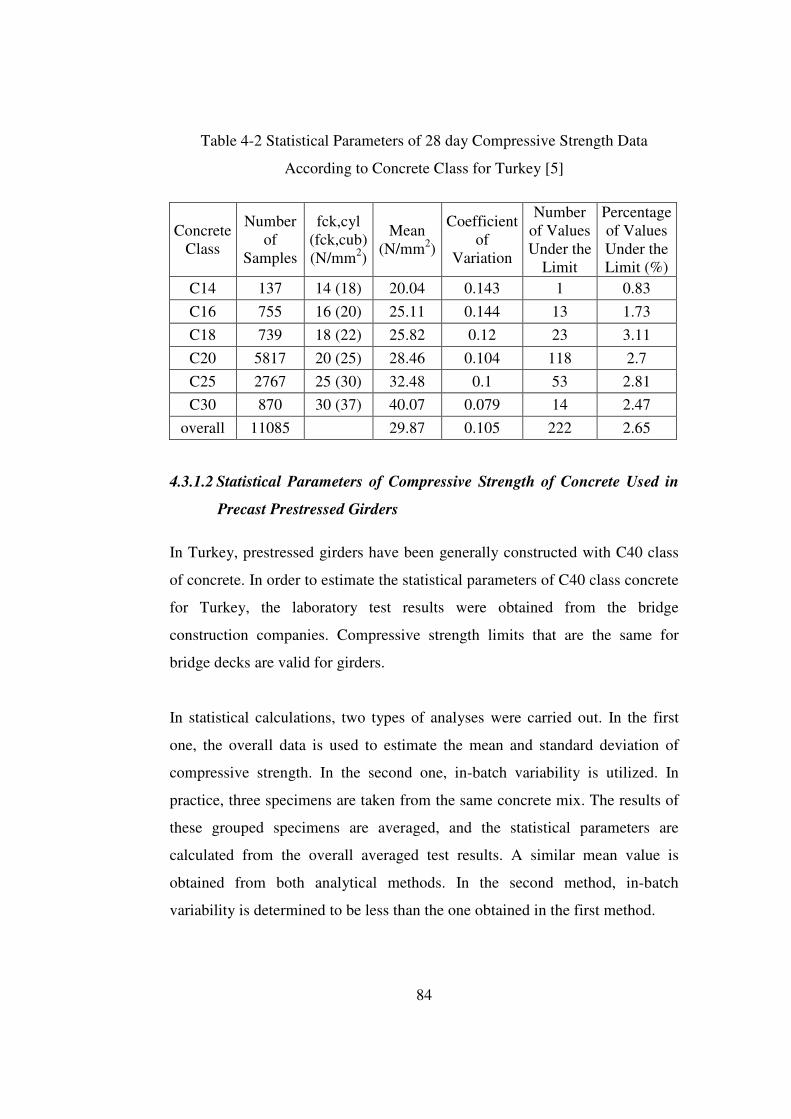
84
Table 4-2 Statistical Parameters of 28 day Compressive Strength Data
According to Concrete Class for Turkey [5]
Concrete Class
Number of
Samples
fck,cyl (fck,cub) (N/mm2)
Mean (N/mm2)
Coefficient of
Variation
Number of Values Under the
Limit
Percentage of Values Under the Limit (%)
C14 137 14 (18) 20.04 0.143 1 0.83
C16 755 16 (20) 25.11 0.144 13 1.73
C18 739 18 (22) 25.82 0.12 23 3.11
C20 5817 20 (25) 28.46 0.104 118 2.7
C25 2767 25 (30) 32.48 0.1 53 2.81
C30 870 30 (37) 40.07 0.079 14 2.47
overall 11085 29.87 0.105 222 2.65
4.3.1.2 Statistical Parameters of Compressive Strength of Concrete Used in
Precast Prestressed Girders
In Turkey, prestressed girders have been generally constructed with C40 class
of concrete. In order to estimate the statistical parameters of C40 class concrete
for Turkey, the laboratory test results were obtained from the bridge
construction companies. Compressive strength limits that are the same for
bridge decks are valid for girders.
In statistical calculations, two types of analyses were carried out. In the first
one, the overall data is used to estimate the mean and standard deviation of
compressive strength. In the second one, in-batch variability is utilized. In
practice, three specimens are taken from the same concrete mix. The results of
these grouped specimens are averaged, and the statistical parameters are
calculated from the overall averaged test results. A similar mean value is
obtained from both analytical methods. In the second method, in-batch
variability is determined to be less than the one obtained in the first method.

85
The twenty-seven standard 150x150x150 mm cube specimens were obtained
from firm 1. All test results of cubic compressive strength were converted to
cylinder compressive strength by dividing cubic strengths by 1.25. The results
are tabulated in Table 4-3. This construction technique is almost standard in
precast concrete industry
According to data from firm 1, 7-day and 28-day mean compressive strengths
are observed to be 39.58 MPa and 47.57 MPa, respectively. In-batch
coefficient of variations for 7-day and 28-day are computed to be 0.043 and
0.026, respectively.
Firm 2 provided with 462 standard 150x300 mm cylinder specimens. The
results are tabulated in Table 4-4. According to data taken from firm 2, 7-day
and 28-day mean compressive strength are computed to be 37.24 MPa and
47.84 MPa, respectively. In-batch coefficient of variations for 7-day and 28-
day are obtained to be 0.084 and 0.066, respectively. Almost the same mean
compressive strength is estimated from tested specimens obtained from firms 1
and 2. Due to a larger sample size, the standard deviation is higher in the
investigated data obtained from firm 2. The seven day concrete compressive
strength is observed to reach to 80% of 28 day strength due to the addition of
chemical additives. This construction technique is almost standard in precast
concrete industry.

86
Table 4-3 Statistical Parameters of 7 and 28 day Laboratory (Cylinder)
Compressive Strength Data of Firm 1 According to C40 Concrete Class
7-Day 28-Day Statistical Parameters
Overall In-Batch Overall In-Batch
Max Value (MPa) 43.30 42.62 50.15 49.17
Min Value (MPa) 35.96 37.59 44.44 45.59
µ, Mean (MPa) 39.58 47.57
σ, Standard Deviation (MPa) 1.86 1.70 1.39 1.26
COV, Coefficient of Variation 0.047 0.043 0.029 0.026
Bias Factor (mean/nominal) - 1.189
Table 4-4 Statistical Parameters of 7 and 28 day Laboratory (Cylinder)
Compressive Strength Data of Firm 2 According to C40 Concrete Class
7. Days 28. Days Statistical Parameters
Overall In-Batch Overall In-Batch
Max Value (MPa) 47.52 44.68 60.2 57.78
Min Value (MPa) 30.85 31.9 40.87 42.72
µ, Mean (MPa) 37.24 47.84
σ, Standard Deviation (MPa) 3.37 3.13 3.66 3.16
COV, Coefficient of Variation 0.090 0.084 0.077 0.066
Bias Factor (mean/nominal) - 1.196
All compressive strength test results obtained from both companies are
combined to estimate the statistical parameters of C40 class concrete.
Combined histograms for 7-day and 28-day compressive strength of C40 are
presented in Figure 4-2 and Figure 4-3 using overall (first method) and in
Figure 4-4 and Figure 4-5 using in-batch analysis (second method). The in-
batch statistical parameters are used in this research, because the concrete mix
used in precast girders is generally supplied only one manufacturer. As
depicted in Table 4-5, the 28 day mean compressive strength is computed to be
47.82 MPa, and in-batch coefficient of variation is 0.064. Mean bias factor for
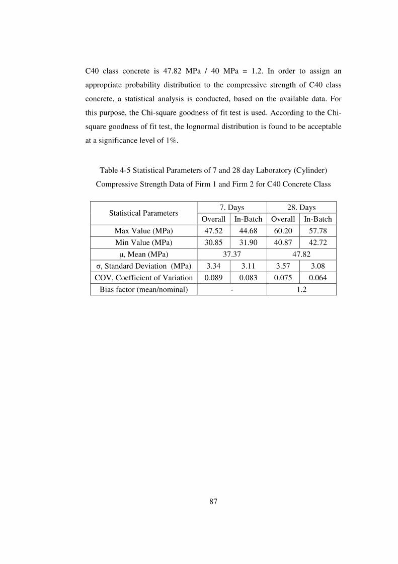
87
C40 class concrete is 47.82 MPa / 40 MPa = 1.2. In order to assign an
appropriate probability distribution to the compressive strength of C40 class
concrete, a statistical analysis is conducted, based on the available data. For
this purpose, the Chi-square goodness of fit test is used. According to the Chi-
square goodness of fit test, the lognormal distribution is found to be acceptable
at a significance level of 1%.
Table 4-5 Statistical Parameters of 7 and 28 day Laboratory (Cylinder)
Compressive Strength Data of Firm 1 and Firm 2 for C40 Concrete Class
7. Days 28. Days Statistical Parameters
Overall In-Batch Overall In-Batch
Max Value (MPa) 47.52 44.68 60.20 57.78
Min Value (MPa) 30.85 31.90 40.87 42.72
µ, Mean (MPa) 37.37 47.82
σ, Standard Deviation (MPa) 3.34 3.11 3.57 3.08
COV, Coefficient of Variation 0.089 0.083 0.075 0.064
Bias factor (mean/nominal) - 1.2

88
0
20
40
60
80
100
120
30 32 34 36 38 40 42 44 46 48 50 52 54 56 58 60
7. Day Concrete Strength (Mpa)
Fre
quen
cy
Figure 4-2 Combined Histogram of 7 Day Laboratory (Cylinder) Compressive
Strength Data (Overall) for C40 Concrete Class
0
20
40
60
80
100
120
30 32 34 36 38 40 42 44 46 48 50 52 54 56 58 60
28. Day Concrete Strength (Mpa)
Fre
quen
cy
Figure 4-3 Combined Histogram of 28 Day Laboratory (Cylinder)
Compressive Strength Data (Overall) for C40 Concrete Class

89
0
10
20
30
40
50
60
30 32 34 36 38 40 42 44 46 48 50 52 54 56 58 60
7. Day Concrete Strength (Mpa)
Fre
quen
cy
Figure 4-4 Combined Histogram of 7 Day Laboratory (Cylinder) Compressive
Strength Data (In-batch) for C40 Concrete Class
0
10
20
30
40
50
60
30 32 34 36 38 40 42 44 46 48 50 52 54 56 58 60
28. Day Concrete Strength (Mpa)
Fre
quen
cy
Figure 4-5 Combined Histogram of 28 Day Laboratory (Cylinder)
Compressive Strength Data (In-batch) for C40 Concrete Class
90
4.3.1.3 Uncertainty Analysis for the Compressive Strength of Concrete
Earlier in this study, the inherent variability (aleatory uncertainty) of
compressive strength of concrete used in bridge decks and precast prestressed
girders are estimated. Besides the inherent variability, additional epistemic
uncertainties can result from the following effects: [5]
• Discrepancies between the laboratory test conditions and in-situ (actual)
conditions,
• Rate of loading,
• Specimens not exactly belonging to actual mix and human errors.
The compressive strength of a cube or a cylinder specimen measured under
laboratory conditions can be higher than the strength of concrete placed in a
member of structure. Different curing and placing processes, the segregation of
concrete, different sizes and shapes and different stress conditions result in
difference in the actual (in-situ) strength and laboratory strength of concrete.
Mirza et al. [6] stated that the average ratio of core strength to actual strength
varies within the range of 0.74 and 0.96 with the prediction (epistemic)
uncertainty of 0.1 expressed in terms of coefficient of variation. [5]
In engineering, information can be expressed in terms of the lower and upper
limits of an uncertain variable in order to convey judgmental information. The
mean value of a variable and the associated uncertainty in terms of coefficient
of variation can be estimated by prescribing a suitable distribution between
these two limits. [8]
The quality control in a bridge construction is usually high compared to the one
in standard building construction. Plant manufactured concrete components can
increase the quality of construction. Therefore, the distribution of the

91
correction factor, 1N , for the difference between laboratory and in-situ strength
can be taken as an upper triangular distribution as shown in Figure 4-6.
Figure 4-6 Upper Triangle Probability Density Function between NL (lower
limit) and NU (upper limit) for N1
The mean value and coefficient of variation can be estimated by the following
expressions [8],
)2(3
1UL NNN ⋅+= (4-16)
+
−=∆
LU
LU
NN
NN
22
1 (4-17)
where, NL is the lower limit and NU is the upper limit of the correction factor.
Mean correction factor, 1N , is calculated as 0.89 and epistemic uncertainty, 1∆
as 0.06, but it is taken as 0.1 as given in [5].
An additional uncertainty is due to the rate of loading in performing the
laboratory tests. If the rate of loading increases, the compressive strength of
concrete will reach higher values than the actual strength. Mirza et al. [6]
accounted for this effect through the correction factor, 2N . The mean value,
2N , is expressed by the following empirical formula.
NL=0.7 NU=0.9x

92
))log(08.01(89.02 RN += (4-18)
where, R is the rate of loading and 2N is the mean correction factor for this
effect. Fırat et al. [5] took 2N as 0.89 and ignored the epistemic uncertainty
associated with 2N . The same values are taken in this study to account for the
uncertainty due to the rate of loading.
One other source of uncertainty is the human error. The specimens can be
taken from a special concrete batch instead of random picks. Moreover,
standard testing procedures may not be conducted. Kömürcü et al. [9]
introduced a prediction error, 3∆ = 0.05 and a mean correction factor, 3N =
0.95 for human induced errors. In this study, the mean correction factor is
taken as 3N =1.0 due to higher quality control in bridge construction.[5]
After evaluating additional uncertainties, the in-situ value of compression
strength of concrete can be modeled by
cfc fNfc
⋅= (4-19)
where, cf is the in-situ value of compressive strength of concrete, cf is the
compressive strength of cylindrical specimens tested at the laboratory, and
cfN is the overall bias in cf . The mean value,
cfN is computed based on the
first-order second moment approximation as:
8.000.189.089.0321 =⋅⋅=⋅⋅= NNNN fc (4-20)

93
Therefore, in-situ compressive strength for C30 class concrete is equal to
32.5x0.8=26 MPa and for C40 class concrete to 47.82x0.8= 38.3 MPa.
The total uncertainty, fcΩ in cf in terms of coefficient of variation can
expressed as:
22 )()( fcfcf c∆+=Ω δ (4-21)
where, fcδ is the inherent (aleatory) uncertainty (calculated in the previous
sections) and fc∆ is the total prediction (epistemic) uncertainty, which is
evaluated as
11.005.001.0 2223
22
21 =++=∆+∆+∆=∆ fc (4-22)
Total uncertainty for C30 class concrete is equal to 135.011.0079.0 22 =+
with the inherent uncertainty, fcδ of 0.079 and for C40 class concrete, it is
equal to 127.011.0064.0 22 =+ . Summary of the statistical parameters of 28
day in-situ compressive strength concrete is presented in Table 4-6. The mean
values of the bias factor, which is the ratio of mean to nominal compressive
strength, for C30 and C40 class concretes, are determined to be 0.87 and 0.96,
respectively.
In the literature, Mirza et al. [18] determined the bias factors as 0.85 and 0.81
and the coefficients of variation as 0.18 and 0.15 for the compressive strength
of 28 MPa and 34.5 MPa class concrete, respectively. In addition, normal
distribution was assumed for the compressive strength of concrete, in that
study. The closest bias factors are calculated if C30 class concrete is compared

94
with C28 class concrete and C40 class concrete is compared with C34.5 class
concrete. The coefficients of variation that calculated in this work are lower
than that found by Mirza.
Table 4-6 Statistical Parameters of (Cylinder) Compressive Strength of C30
and C40 Concrete Class
Concrete Class Statistical Parameters
C30 C40
Laboratory Measured Mean (MPa)
32.5 47.8
In-situ Mean (MPa) 26.0 38.3
Standard Deviation (MPa) 3.5 4.9
Coefficient of Variation 0.135 0.127
Nominal (MPa) 30.0 40.0
Bias Factor (mean/nominal) 0.87 0.96
4.3.2 Prestressing Strand
Seven-wire strand is the most common prestressing type used in the
construction of bridge girders. There are two types of seven-wire strands based
on the manufacturing process they go through; stress-relieved and low-
relaxation strand. Seven-wire strand is produced by wrapping six wires around
one central wire in a helical manner. The residual stress is formed in untreated
strands due to cooling and twisting of wires during the process, and this causes
a decrease in yield stress. The strands are heated to 350°C, and as they are
allowed to cool slowly in order to eliminate the residual stresses and increase
the yield strength of strand, this process is called stress relieving. In another
type of manufacturing process, the strands are put into tension during the
heating and cooling process in order to reduce the relaxation of the strands. The
strand produced by this method is called low-relaxation strand. [4]
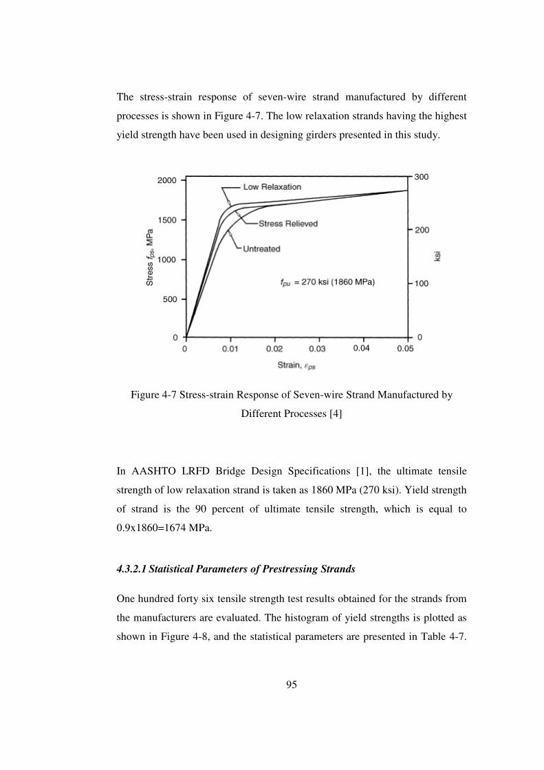
95
The stress-strain response of seven-wire strand manufactured by different
processes is shown in Figure 4-7. The low relaxation strands having the highest
yield strength have been used in designing girders presented in this study.
Figure 4-7 Stress-strain Response of Seven-wire Strand Manufactured by
Different Processes [4]
In AASHTO LRFD Bridge Design Specifications [1], the ultimate tensile
strength of low relaxation strand is taken as 1860 MPa (270 ksi). Yield strength
of strand is the 90 percent of ultimate tensile strength, which is equal to
0.9x1860=1674 MPa.
4.3.2.1 Statistical Parameters of Prestressing Strands
One hundred forty six tensile strength test results obtained for the strands from
the manufacturers are evaluated. The histogram of yield strengths is plotted as
shown in Figure 4-8, and the statistical parameters are presented in Table 4-7.

96
The mean of yield strength of prestressing strands is computed as 1740 MPa
and coefficient of variation as 0.021. The mean bias factor is 1740/1674=1.04.
0
10
20
30
40
50
60
1575 1600 1625 1650 1675 1700 1725 1750 1775
Yield Strengths of Prestressing Strand (MPa)
Fre
quen
cy
Figure 4-8 Histogram of Laboratory Yield Strength of Strands
Table 4-7 Statistical Parameters of Laboratory Yield Strength of Strand
Statistical Parameters Values
Max Value (MPa) 1781
Min Value (MPa) 1599
µ, Mean (MPa) 1740
σ, Standard Deviation (MPa) 36.29
COV, Coefficient of Variation 0.021
Bias Factor (mean/nominal) 1.04
Mirza et al. [19] evaluated the statistical parameters of yield strength of
prestressing strands by using 200 test records of the manufacturers. In his
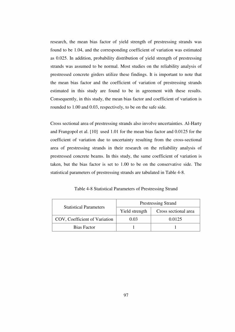
97
research, the mean bias factor of yield strength of prestressing strands was
found to be 1.04, and the corresponding coefficient of variation was estimated
as 0.025. In addition, probability distribution of yield strength of prestressing
strands was assumed to be normal. Most studies on the reliability analysis of
prestressed concrete girders utilize these findings. It is important to note that
the mean bias factor and the coefficient of variation of prestressing strands
estimated in this study are found to be in agreement with these results.
Consequently, in this study, the mean bias factor and coefficient of variation is
rounded to 1.00 and 0.03, respectively, to be on the safe side.
Cross sectional area of prestressing strands also involve uncertainties. Al-Harty
and Frangopol et al. [10] used 1.01 for the mean bias factor and 0.0125 for the
coefficient of variation due to uncertainty resulting from the cross-sectional
area of prestressing strands in their research on the reliability analysis of
prestressed concrete beams. In this study, the same coefficient of variation is
taken, but the bias factor is set to 1.00 to be on the conservative side. The
statistical parameters of prestressing strands are tabulated in Table 4-8.
Table 4-8 Statistical Parameters of Prestressing Strand
Prestressing Strand Statistical Parameters
Yield strength Cross sectional area
COV, Coefficient of Variation 0.03 0.0125
Bias Factor 1 1
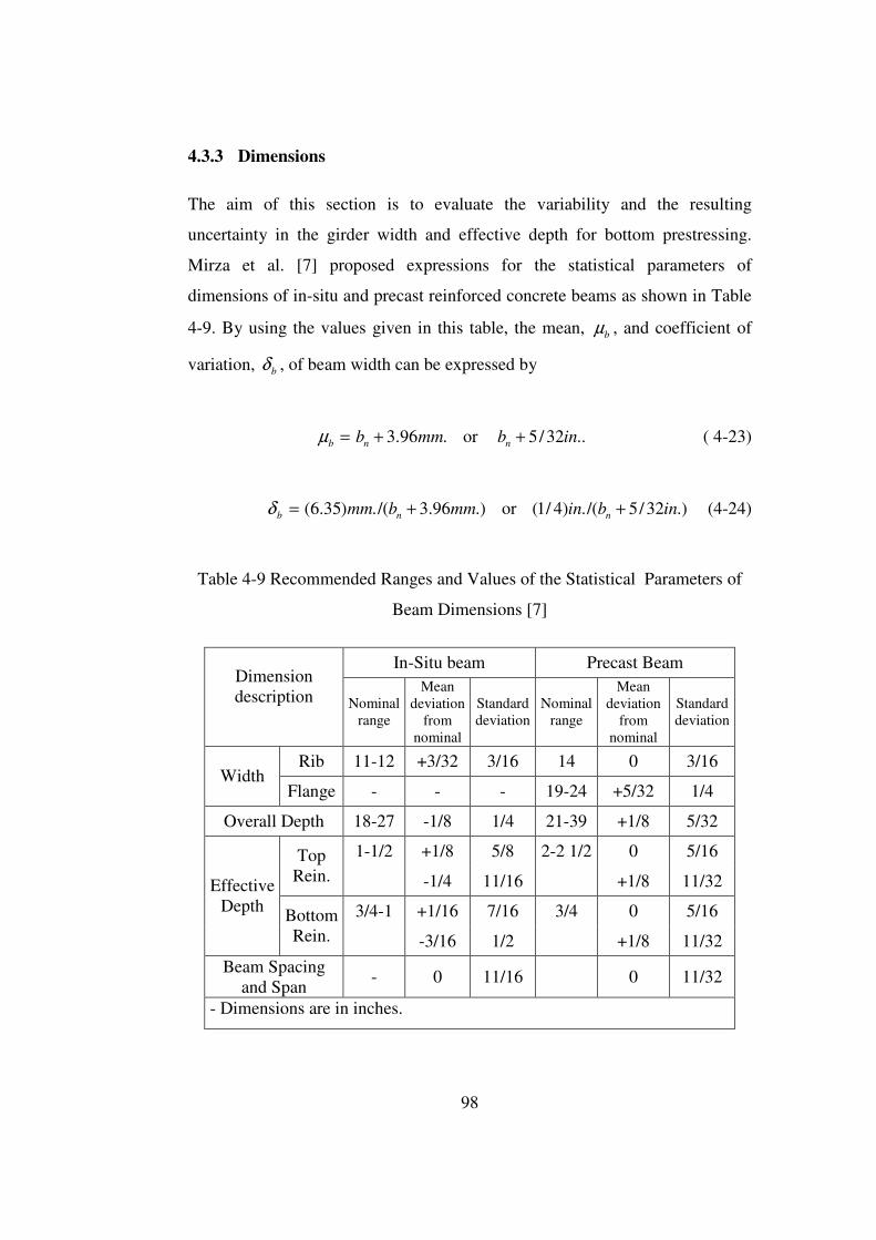
98
4.3.3 Dimensions
The aim of this section is to evaluate the variability and the resulting
uncertainty in the girder width and effective depth for bottom prestressing.
Mirza et al. [7] proposed expressions for the statistical parameters of
dimensions of in-situ and precast reinforced concrete beams as shown in Table
4-9. By using the values given in this table, the mean, bµ , and coefficient of
variation, bδ , of beam width can be expressed by
=bµ .96.3 mmbn + or ..32/5 inbn + ( 4-23)
=bδ .)96.3/(.)35.6( mmbmm n + or .)32/5/(.)4/1( inbin n + (4-24)
Table 4-9 Recommended Ranges and Values of the Statistical Parameters of
Beam Dimensions [7]
In-Situ beam Precast Beam Dimension description
Nominal
range
Mean deviation
from nominal
Standard deviation
Nominal range
Mean deviation
from nominal
Standard deviation
Rib 11-12 +3/32 3/16 14 0 3/16 Width
Flange - - - 19-24 +5/32 1/4
Overall Depth 18-27 -1/8 1/4 21-39 +1/8 5/32
1-1/2 +1/8 5/8 2-2 1/2 0 5/16 Top Rein. -1/4 11/16 +1/8 11/32
3/4-1 +1/16 7/16 3/4 0 5/16
Effective Depth
Bottom Rein. -3/16 1/2 +1/8 11/32
Beam Spacing and Span
- 0 11/16 0 11/32
- Dimensions are in inches.
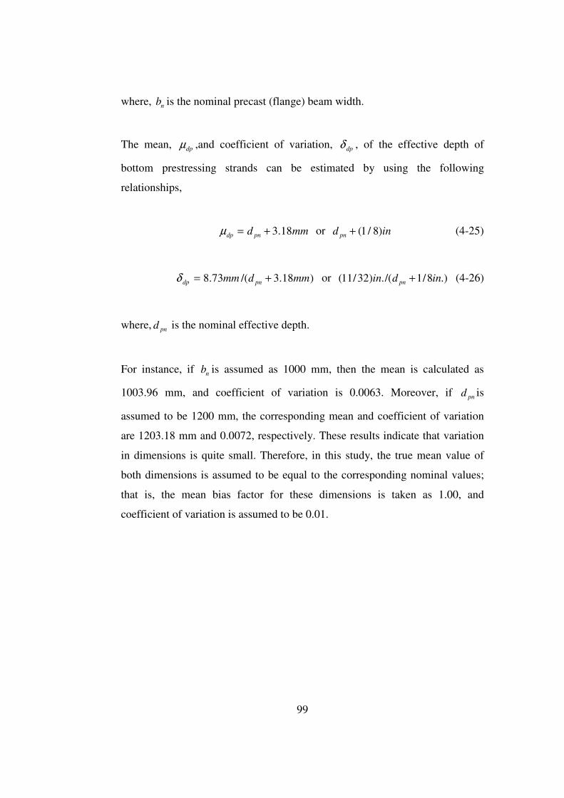
99
where, nb is the nominal precast (flange) beam width.
The mean, dpµ ,and coefficient of variation, dpδ , of the effective depth of
bottom prestressing strands can be estimated by using the following
relationships,
=dpµ mmd pn 18.3+ or ind pn )8/1(+ (4-25)
=dpδ )18.3/(73.8 mmdmm pn + or .)8/1/(.)32/11( indin pn + (4-26)
where, pnd is the nominal effective depth.
For instance, if nb is assumed as 1000 mm, then the mean is calculated as
1003.96 mm, and coefficient of variation is 0.0063. Moreover, if pnd is
assumed to be 1200 mm, the corresponding mean and coefficient of variation
are 1203.18 mm and 0.0072, respectively. These results indicate that variation
in dimensions is quite small. Therefore, in this study, the true mean value of
both dimensions is assumed to be equal to the corresponding nominal values;
that is, the mean bias factor for these dimensions is taken as 1.00, and
coefficient of variation is assumed to be 0.01.
100
4.4 SUMMARY OF THE STATISTICAL PARAMETERS OF
RESISTANCE
The probability distributions, coefficients of variation and mean bias factor
values of the resistance parameters that are assessed in the previous sections
are summarized in Table 4-10. k and β1 are assumed to be deterministic
quantities. PF denotes the professional factor that describes the uncertainty
resulting from the use of approximate resistance and idealized stress and strain
models [12].
Table 4-10 Summary of Statistical Parameters of Resistance
Parameter Description Probability Distribution
Bias Factor
Coefficient of Variation
Aps Area of prestressing strand
Normal 1.0 0.0125
fpu Ultimate tensile strength of prestressing steel
Normal 1.0 0.03
fc,C30 Compression strength of deck concrete
Normal 0.87 0.135
fc,C40 Compression strength of precast beam
Lognormal 0.96 0.127
dp
Distance from extreme compression fiber to the centroid of prestressing steel
Normal 1.0 0.010
b Width of compression flange
Normal 1.0 0.010
k 0.28 for low relaxation strands
- - -
β1 Stress factor for compression block
- - -
PF Professional factor Normal 1.01 0.06
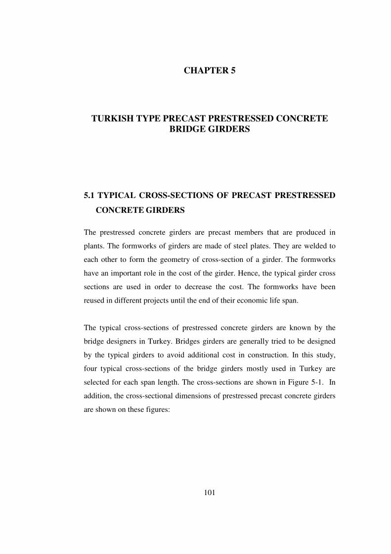
101
CHAPTER 5
TURKISH TYPE PRECAST PRESTRESSED CONCRETE BRIDGE GIRDERS
5.1 TYPICAL CROSS-SECTIONS OF PRECAST PRESTRESSED
CONCRETE GIRDERS
The prestressed concrete girders are precast members that are produced in
plants. The formworks of girders are made of steel plates. They are welded to
each other to form the geometry of cross-section of a girder. The formworks
have an important role in the cost of the girder. Hence, the typical girder cross
sections are used in order to decrease the cost. The formworks have been
reused in different projects until the end of their economic life span.
The typical cross-sections of prestressed concrete girders are known by the
bridge designers in Turkey. Bridges girders are generally tried to be designed
by the typical girders to avoid additional cost in construction. In this study,
four typical cross-sections of the bridge girders mostly used in Turkey are
selected for each span length. The cross-sections are shown in Figure 5-1. In
addition, the cross-sectional dimensions of prestressed precast concrete girders
are shown on these figures:

102
Figure 5-1 Cross-Sections of the Typical Prestressed Precast Concrete Girders
Conducted in Turkey (dimensions are in cm.)
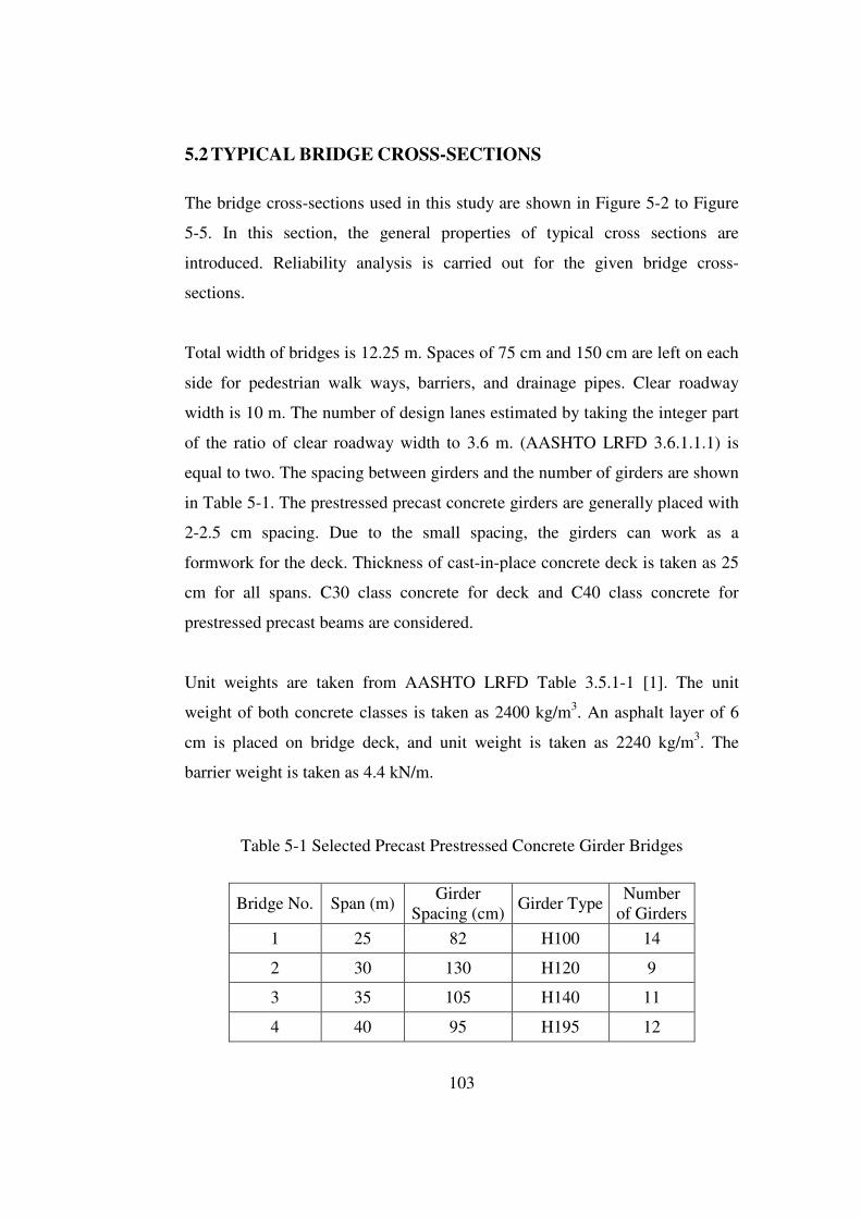
103
5.2 TYPICAL BRIDGE CROSS-SECTIONS
The bridge cross-sections used in this study are shown in Figure 5-2 to Figure
5-5. In this section, the general properties of typical cross sections are
introduced. Reliability analysis is carried out for the given bridge cross-
sections.
Total width of bridges is 12.25 m. Spaces of 75 cm and 150 cm are left on each
side for pedestrian walk ways, barriers, and drainage pipes. Clear roadway
width is 10 m. The number of design lanes estimated by taking the integer part
of the ratio of clear roadway width to 3.6 m. (AASHTO LRFD 3.6.1.1.1) is
equal to two. The spacing between girders and the number of girders are shown
in Table 5-1. The prestressed precast concrete girders are generally placed with
2-2.5 cm spacing. Due to the small spacing, the girders can work as a
formwork for the deck. Thickness of cast-in-place concrete deck is taken as 25
cm for all spans. C30 class concrete for deck and C40 class concrete for
prestressed precast beams are considered.
Unit weights are taken from AASHTO LRFD Table 3.5.1-1 [1]. The unit
weight of both concrete classes is taken as 2400 kg/m3. An asphalt layer of 6
cm is placed on bridge deck, and unit weight is taken as 2240 kg/m3. The
barrier weight is taken as 4.4 kN/m.
Table 5-1 Selected Precast Prestressed Concrete Girder Bridges
Bridge No. Span (m) Girder
Spacing (cm) Girder Type
Number of Girders
1 25 82 H100 14
2 30 130 H120 9
3 35 105 H140 11
4 40 95 H195 12
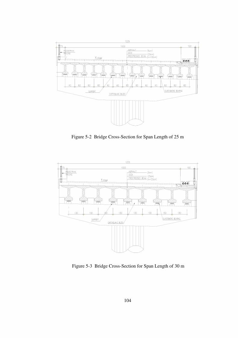
104
Figure 5-2 Bridge Cross-Section for Span Length of 25 m
Figure 5-3 Bridge Cross-Section for Span Length of 30 m
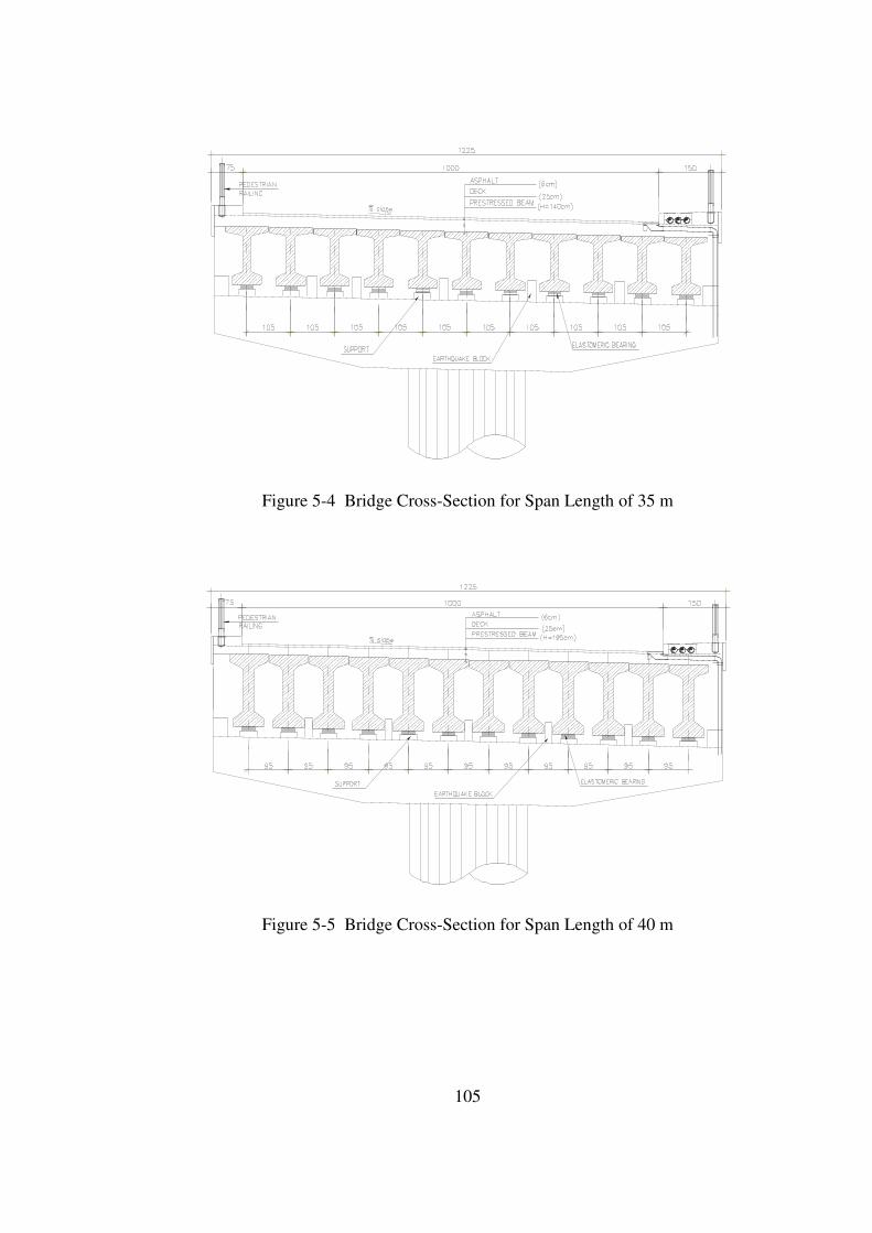
105
Figure 5-4 Bridge Cross-Section for Span Length of 35 m
Figure 5-5 Bridge Cross-Section for Span Length of 40 m
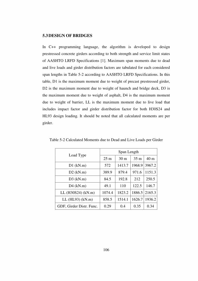
106
5.3 DESIGN OF BRIDGES
In C++ programming language, the algorithm is developed to design
prestressed concrete girders according to both strength and service limit states
of AASHTO LRFD Specifications [1]. Maximum span moments due to dead
and live loads and girder distribution factors are tabulated for each considered
span lengths in Table 5-2 according to AASHTO LRFD Specifications. In this
table, D1 is the maximum moment due to weight of precast prestressed girder,
D2 is the maximum moment due to weight of haunch and bridge deck, D3 is
the maximum moment due to weight of asphalt, D4 is the maximum moment
due to weight of barrier, LL is the maximum moment due to live load that
includes impact factor and girder distribution factor for both H30S24 and
HL93 design loading. It should be noted that all calculated moments are per
girder.
Table 5-2 Calculated Moments due to Dead and Live Loads per Girder
Span Length Load Type
25 m 30 m 35 m 40 m
D1 (kN.m) 572 1413.7 1968.9 3967.2
D2 (kN.m) 389.9 879.4 971.6 1151.3
D3 (kN.m) 84.5 192.8 212 250.5
D4 (kN.m) 49.1 110 122.5 146.7
LL (H30S24) (kN.m) 1074.4 1823.2 1886.5 2165.3
LL (HL93) (kN.m) 858.5 1514.1 1626.7 1936.2
GDF, Girder Distr. Func. 0.29 0.4 0.35 0.34

107
The aim of the design is to determine the minimum required number of
prestressing strands for the identified cross-section, material property and span
length. The required number of prestressing strands for strength I limit state
shall satisfy the minimum required resistance corresponding to the factored
flexural moment demand at the investigated section. Flexural resistance
capacity (R) is calculated as explained in Section 4.1, and minimum required
resistance (Rmin) is calculated by multiplying the moment due to dead and live
load effects by each corresponding load factors of strength I limit state by Eq.
4.1. The number of prestressing strands required for service III limit state shall
prevent cracking at the bottom fiber (see chapter 4.2). The design of
prestressed concrete girders is done by the program developed as a part of this
research. The results are shown for both design loadings and the considered
span lengths and for both strength and service limit states in Table 5-3 to Table
5-6.
Table 5-3 Results of Design According to Strength I Limit State for H30S24
Span Length Parameters
25 m 30 m 35 m 40 m
Rmin (kN.m) 3283.1 6511.3 7478.7 10783.1
R (kN.m) 3416.4 6691.9 7627.3 10861
Max Tensile Stress Limit (MPa) 3.162 3.162 3.162 3.162
Tensile Stress at Bottom (MPa) 3.771 4.842 5.177 4.54
Number of Strands 18 30 30 31
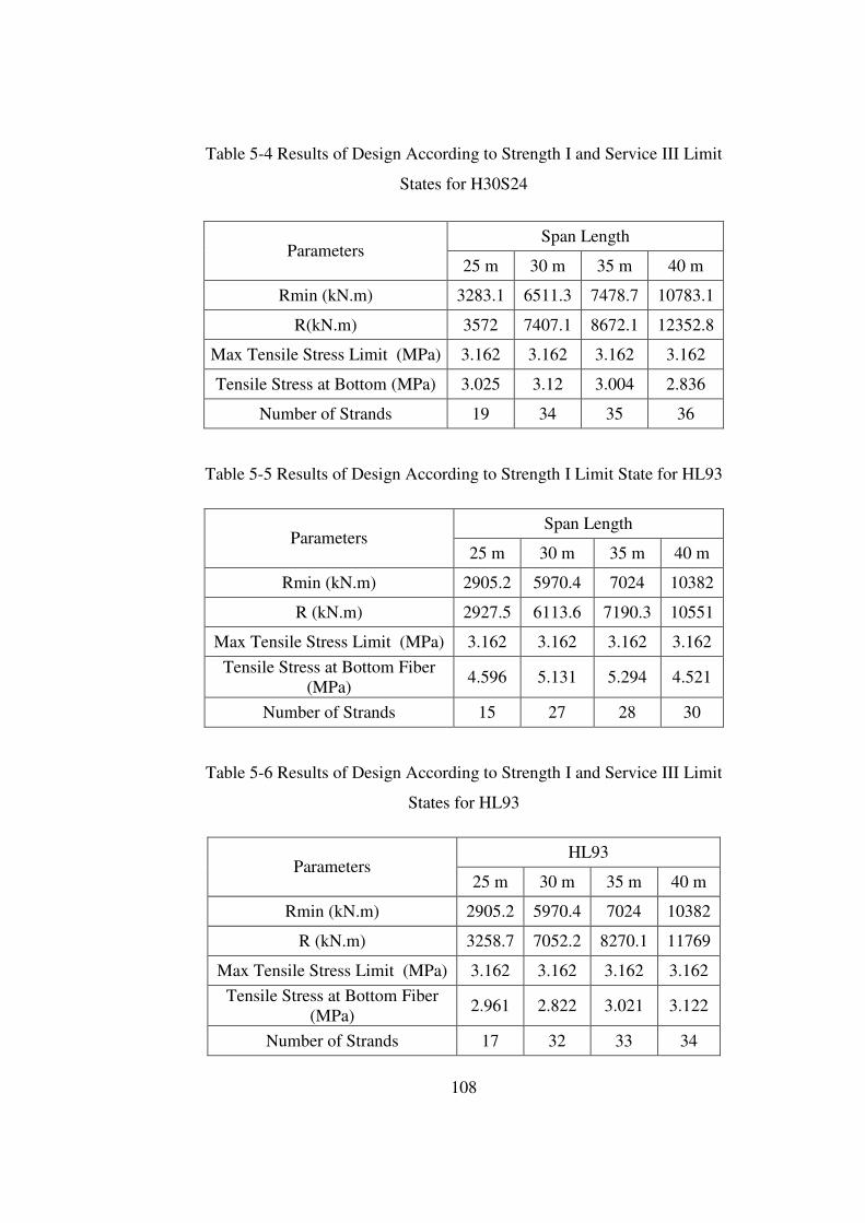
108
Table 5-4 Results of Design According to Strength I and Service III Limit
States for H30S24
Span Length Parameters
25 m 30 m 35 m 40 m
Rmin (kN.m) 3283.1 6511.3 7478.7 10783.1
R(kN.m) 3572 7407.1 8672.1 12352.8
Max Tensile Stress Limit (MPa) 3.162 3.162 3.162 3.162
Tensile Stress at Bottom (MPa) 3.025 3.12 3.004 2.836
Number of Strands 19 34 35 36
Table 5-5 Results of Design According to Strength I Limit State for HL93
Span Length Parameters
25 m 30 m 35 m 40 m
Rmin (kN.m) 2905.2 5970.4 7024 10382
R (kN.m) 2927.5 6113.6 7190.3 10551
Max Tensile Stress Limit (MPa) 3.162 3.162 3.162 3.162
Tensile Stress at Bottom Fiber (MPa)
4.596 5.131 5.294 4.521
Number of Strands 15 27 28 30
Table 5-6 Results of Design According to Strength I and Service III Limit
States for HL93
HL93 Parameters
25 m 30 m 35 m 40 m
Rmin (kN.m) 2905.2 5970.4 7024 10382
R (kN.m) 3258.7 7052.2 8270.1 11769
Max Tensile Stress Limit (MPa) 3.162 3.162 3.162 3.162
Tensile Stress at Bottom Fiber (MPa)
2.961 2.822 3.021 3.122
Number of Strands 17 32 33 34

109
The required number of prestressing strands is plotted in Figure 5-6. H30S24
design truck model results in a higher number of prestressing strands in both
limit states compared to the HL-93 truck model. In addition, the number of
prestressing strands required by service III limit state is typically more than the
minimum number of strands required by the strength I limit state. Strand ratio,
calculated by dividing the minimum required number of strands determined in
service III limit state to the ones determined in strength I limit state, is adopted
for comparison. If strand ratio is greater than 1, it means that there is an
additional factor of safety the prestressed concrete bridge girders possess
beyond the minimum value required by the strength limit state [17] as depicted
in Figure 5-7. The average additional safety is around %15 and %13 for HL93
and H30S24, respectively.
10
15
20
25
30
35
40
20 25 30 35 40 45
Span Length (m)
Num
ber
Of
Str
ands
.
H30S24-Strength
H30S24-Service
HL93-Strength
HL93-Service
Figure 5-6 Number of Strands per Girder for Strength I and Service III Limit
States
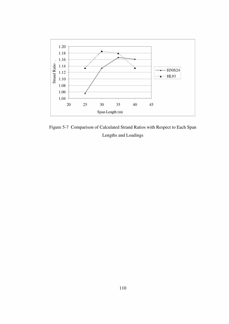
110
1.04
1.06
1.08
1.10
1.12
1.14
1.16
1.18
1.20
20 25 30 35 40 45
Span Length (m)
Str
and
Rat
io .
H30S24
HL93
Figure 5-7 Comparison of Calculated Strand Ratios with Respect to Each Span
Lengths and Loadings

111
CHAPTER 6
RELIABILITY-BASED SAFETY LEVEL EVALUATION
6.1 LIMIT STATE FUNCTION
There are many ways and modes of failure of bridges. These are cracking,
corrosion, excessive deformations, exceeding the carrying capacity for shear or
bending moment, local or overall buckling. A traditional notion of the safety
limit is associated with the ultimate limit states which is the ultimate bending
(flexural) moment capacity.[12]
Let R be the resistance (moment carrying capacity in this case) and Q
represents the load effect (total moment applied to considered beam) then, the
limit state function, g, can be expressed by
QRg −= (6-1)
If 0>g , the structure is safe; otherwise it fails. The probability of failure, FP
is defined as,
)0()0( <=<−= gPQRPPF (6-2)
In this study, total load effect is expressed by
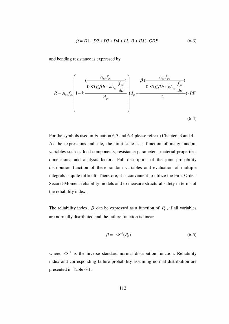
112
GDFIMLLDDDDQ ⋅+⋅++++= )1(4321 (6-3)
and bending resistance is expressed by
PFdp
fkAbf
fA
dd
dp
fkAbf
fA
kfAR
pu
psc
pups
p
p
pu
psc
pups
pups ⋅
+′
−
+′
−= )2
)
85.0
(
(
)
85.0
(
11
1
1 β
β
β
(6-4)
For the symbols used in Equation 6-3 and 6-4 please refer to Chapters 3 and 4.
As the expressions indicate, the limit state is a function of many random
variables such as load components, resistance parameters, material properties,
dimensions, and analysis factors. Full description of the joint probability
distribution function of these random variables and evaluation of multiple
integrals is quite difficult. Therefore, it is convenient to utilize the First-Order-
Second-Moment reliability models and to measure structural safety in terms of
the reliability index.
The reliability index, β can be expressed as a function of FP , if all variables
are normally distributed and the failure function is linear.
)(1FP−Φ−=β (6-5)
where, 1−Φ is the inverse standard normal distribution function. Reliability
index and corresponding failure probability assuming normal distribution are
presented in Table 6-1.
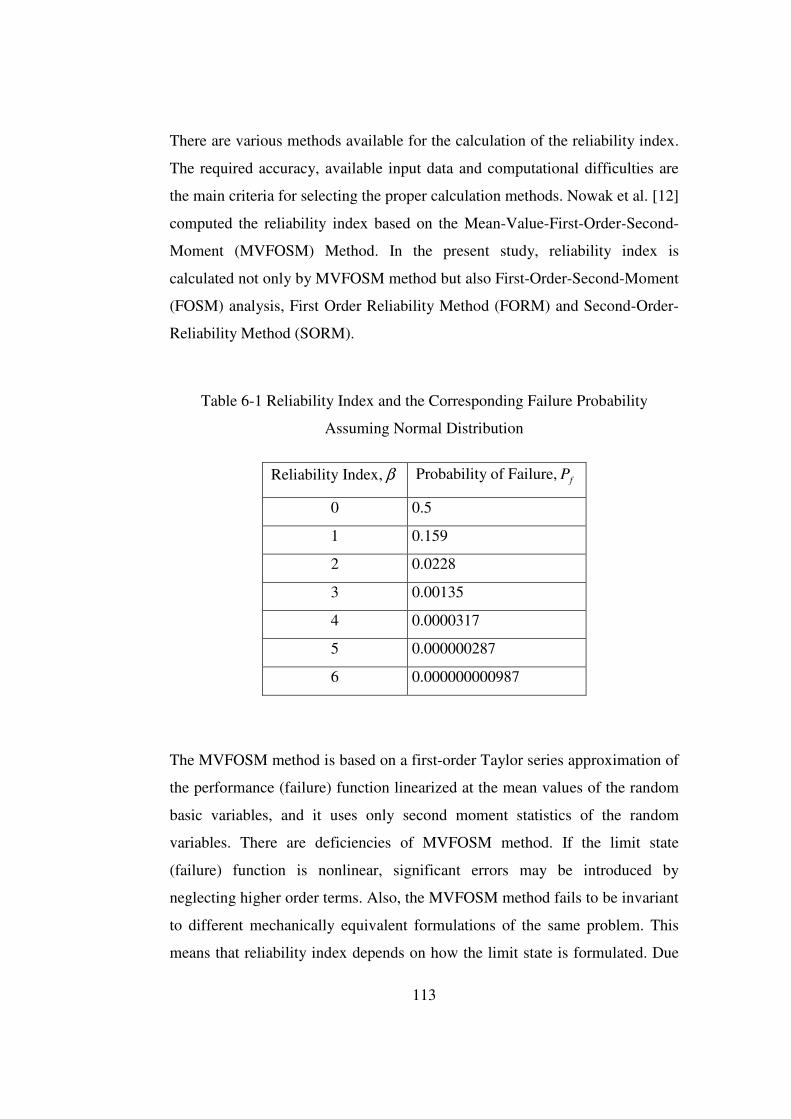
113
There are various methods available for the calculation of the reliability index.
The required accuracy, available input data and computational difficulties are
the main criteria for selecting the proper calculation methods. Nowak et al. [12]
computed the reliability index based on the Mean-Value-First-Order-Second-
Moment (MVFOSM) Method. In the present study, reliability index is
calculated not only by MVFOSM method but also First-Order-Second-Moment
(FOSM) analysis, First Order Reliability Method (FORM) and Second-Order-
Reliability Method (SORM).
Table 6-1 Reliability Index and the Corresponding Failure Probability
Assuming Normal Distribution
Reliability Index, β Probability of Failure, fP
0 0.5
1 0.159
2 0.0228
3 0.00135
4 0.0000317
5 0.000000287
6 0.000000000987
The MVFOSM method is based on a first-order Taylor series approximation of
the performance (failure) function linearized at the mean values of the random
basic variables, and it uses only second moment statistics of the random
variables. There are deficiencies of MVFOSM method. If the limit state
(failure) function is nonlinear, significant errors may be introduced by
neglecting higher order terms. Also, the MVFOSM method fails to be invariant
to different mechanically equivalent formulations of the same problem. This
means that reliability index depends on how the limit state is formulated. Due

114
to these shortcomings of the MVFOSM method, Hasofer and Lind [26]
proposed a new reliability index, 2β . The process of calculating 2β is generally
referred as the advanced first-order second moment method (FOSM).
Reliability index 2β is defined as the shortest distance from the origin to the
failure surface in the z-coordinate system, and the design point is defined as the
point having the shortest distance to the origin on the failure surface (see
Figure 6-1). When the failure surface is nonlinear, the search for the design
point and the calculation of the reliability index is carried out by an iterative
algorithm.[5]
Figure 6-1 Description of Reliability Index 2β [5]
FORM is an analytical approximation in which the reliability index is
interpreted as the minimum distance from the origin to the limit state surface in
standardized normal space (z-space). The performance function is
approximated by a linear function in the z-space at the design point, accuracy
problems occur when the performance function is strongly nonlinear. The

115
second-order reliability method (SORM) has been established as an attempt to
improve the accuracy of FORM. SORM is obtained by approximating the limit
state surface in the z-space at the design point by a second-order surface. In
SORM, the difficult, time consuming portion is the computation of the matrix
of second-order derivatives. [25]
Since the exact computation of the failure probability is quite complicated,
numerous studies have contributed to develop some approximations that have
closed forms, the accuracy of which is generally dependent on the three
parameters of the limit state surface, i.e. the curvature radius R at the design
point, the number of random variables n and the first-order reliability index.
Breitung [27] has derived an asymptotic formula which approaches the exact
failure probability as ∞→Fβ with iF kβ , where ik is a principal curvature at
the design point, fixed. [25] However, such methods are not considered in this
study and reliability index is computed by using MVFOSM, FOSM, FORM
and SORM.
6.2 RELIABILITY LEVEL ACCORDING TO AASHTO LRFD
BASED ON LOCAL CONDITIONS
The reliability indexes are calculated according to AASHTO LRFD [1] by
using statistical parameters of load and resistance variables that were assessed
in the previous sections (see Table 4-10 and Table 3-26) reflecting the
conditions of Turkey. In these computations four different reliability analysis
methods, namely MVFOSM, FOSM, FORM and SORM are used. Both service
and strength limit states are considered. The results are tabulated in Table 6-2.
As the results demonstrate, the calculated reliability indexes vary according to
the chosen method. In this study, minimum reliability index is chosen among
the reliability indexes calculated by different methods for each case. In general,

116
the reliability indexes calculated by the Second-Order-Reliability Method
(SORM) are observed to be lower than these obtained from the others.
Reliability indexes calculated based on the statistical parameters reflecting the
local conditions for service and strength limit states are plotted in Figure 6-2.
The reliability indexes based on the requirements of strength limit state are
observed to vary between 4.48-4.21 for girders designed according to H30S24
loading and between 3.92-3.67 for girders designed according to HL93
loading. Moreover, the reliability indexes calculated based on the requirements
of service limit state lie between 4.91-5.33 for girders designed according to
H30S24 loading and 4.59-4.73 for girders designed according to HL93 loading.
The results indicate that reliability indexes of girders designed by H30S24
loading result in a higher reliability index than the ones designed by HL93 for
strength and service limit states. Designs according to service limit state result
in higher reliability indexes due to providing extra safety in design in this limit
state.
The reliability indexes are calculated according to AASHTO LRFD [1] by
using statistical parameters of load and resistance variables that were taken
from calibration report [12] reflecting the conditions of USA. The results are
shown in Figure 6-3. It is concluded that the reliability indexes reflecting the
conditions of USA are observed to be lower in comparison with that reflecting
the conditions of Turkey.
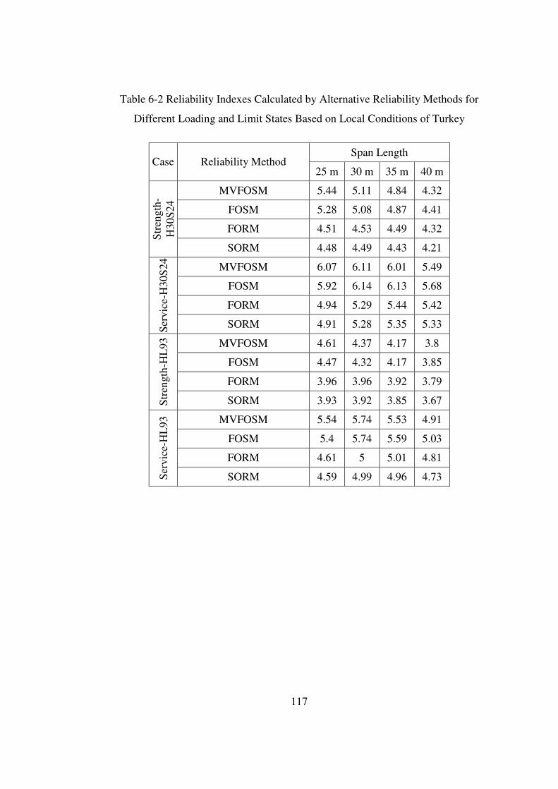
117
Table 6-2 Reliability Indexes Calculated by Alternative Reliability Methods for
Different Loading and Limit States Based on Local Conditions of Turkey
Span Length Case Reliability Method
25 m 30 m 35 m 40 m
MVFOSM 5.44 5.11 4.84 4.32
FOSM 5.28 5.08 4.87 4.41
FORM 4.51 4.53 4.49 4.32
Str
engt
h-H
30S
24
SORM 4.48 4.49 4.43 4.21
MVFOSM 6.07 6.11 6.01 5.49
FOSM 5.92 6.14 6.13 5.68
FORM 4.94 5.29 5.44 5.42
Ser
vice
-H30
S24
SORM 4.91 5.28 5.35 5.33
MVFOSM 4.61 4.37 4.17 3.8
FOSM 4.47 4.32 4.17 3.85
FORM 3.96 3.96 3.92 3.79
Str
engt
h-H
L93
SORM 3.93 3.92 3.85 3.67
MVFOSM 5.54 5.74 5.53 4.91
FOSM 5.4 5.74 5.59 5.03
FORM 4.61 5 5.01 4.81
Ser
vice
-HL
93
SORM 4.59 4.99 4.96 4.73

118
0.00
1.00
2.00
3.00
4.00
5.00
6.00
25.00 30.00 35.00 40.00
Span Length (m)
Rel
iabi
lity
Inde
x .
Strength-H30S24
Service-H30S24
Strenght-HL93
Service-HL93
Figure 6-2 Variation of Reliability Indexes with Span Lengths Considering the
Local Conditions in Turkey
0.00
1.00
2.00
3.00
4.00
5.00
6.00
25.00 30.00 35.00 40.00
Span Length (m)
Rel
iabi
lity
Inde
x .
Strength-H30S24
Service-H30S24
Strenght-HL93
Service-HL93
Figure 6-3 Variation of Reliability Indexes with Span Lengths Considering the
Local Conditions in USA

119
6.3 COMPARISON WITH OTHER DESING CODES AND
COUNTRIES
Similar studies have been carried out for different design codes consistent with
the uncertainties existing in the design practice of different countries. The
countries considered in this section are Spain [3] and China [17]. Reliability
indexes taken from such studies are summarized in Table 6-3, and the results
are plotted in Figure 6-5. Note that, in this table and figure, the first entry is the
country name that the statistical parameters of load and resistance variables are
based on, and the second entry is the design code used.
Reliability index is highly dependent on the statistical parameters of load and
resistance variables, assumptions and method of analysis. Before comparison
of the reliability indexes of girders designed by other specifications and
corresponding to other local conditions, the difference between the studies
from which reliability indexes are taken should be determined. For this
purpose, the reliability indexes reflecting the designs by AASHTO LRFD and
local conditions of USA that are determined from each study are compared and
the values are plotted in Figure 6-4. Note that, in this figure, the word in
parenthesis refers to the county that the study is carried out. It is expected that
the reliability indexes are close to each other because of using same design
code and same statistical parameters of load and resistance components.
However, the Spanish and Chinese researchers found higher reliability indexes
than that estimated in the calibration report. So, the reliability levels calculated
in these researches may be higher than actual level due to taking into different
statistical parameters and assumptions.
As Figure 6-5 indicates, the reliability levels of girders of Turkey for both
loadings are higher than that of girders designed by AASHTO LRFD and
HONG KONG CODE [17] using the statistical parameters of load and
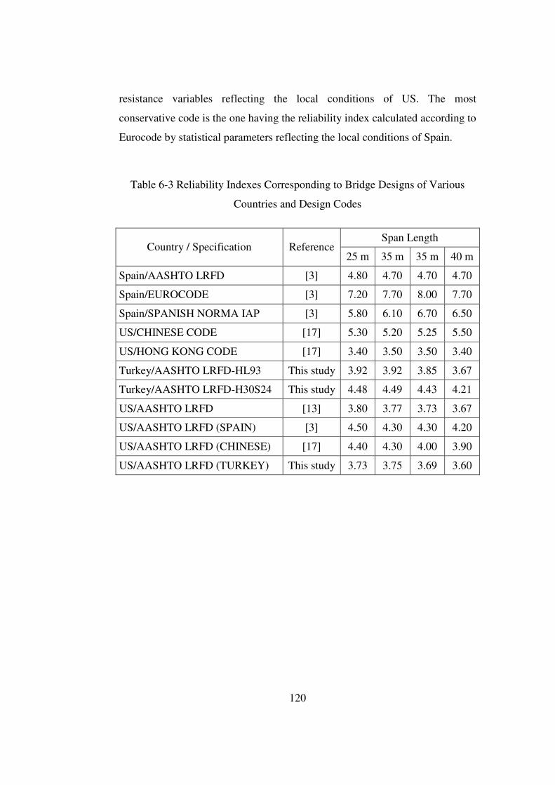
120
resistance variables reflecting the local conditions of US. The most
conservative code is the one having the reliability index calculated according to
Eurocode by statistical parameters reflecting the local conditions of Spain.
Table 6-3 Reliability Indexes Corresponding to Bridge Designs of Various
Countries and Design Codes
Span Length Country / Specification Reference
25 m 35 m 35 m 40 m
Spain/AASHTO LRFD [3] 4.80 4.70 4.70 4.70
Spain/EUROCODE [3] 7.20 7.70 8.00 7.70
Spain/SPANISH NORMA IAP [3] 5.80 6.10 6.70 6.50
US/CHINESE CODE [17] 5.30 5.20 5.25 5.50
US/HONG KONG CODE [17] 3.40 3.50 3.50 3.40
Turkey/AASHTO LRFD-HL93 This study 3.92 3.92 3.85 3.67
Turkey/AASHTO LRFD-H30S24 This study 4.48 4.49 4.43 4.21
US/AASHTO LRFD [13] 3.80 3.77 3.73 3.67
US/AASHTO LRFD (SPAIN) [3] 4.50 4.30 4.30 4.20
US/AASHTO LRFD (CHINESE) [17] 4.40 4.30 4.00 3.90
US/AASHTO LRFD (TURKEY) This study 3.73 3.75 3.69 3.60

121
3
4
5
6
25 m 35 m 35 m 40 mSpan Length (m)
Rel
iabi
lity
Inde
x .
CalibrationRep/AASHTOLRFD
US/AASHTO LRFD(SPAIN)
US/AASHTO LRFD(CHINESE)
US/AASHTO LRFD(TURKEY)
Figure 6-4 Comparison of Reliability Indexes Based on Calibration Report of
AASHTO LRFD as Calculated by Different Studies

122
2
3
4
5
6
7
8
9
25 m 35 m 35 m 40 m
Span Length (m)
Rel
iabi
lity
Inde
x .
Spain/AASHTO LRFD
Spain/EUROCODE
Spain/SPANISH NORMA IAP
US/CHINESE CODE
US/HONG KONG CODE
Turkey/AASHTO LRFD-HL93
Turkey/AASHTO LRFD-H30S24
US/AASHTO LRFD
Figure 6-5 Comparison of Reliability Indexes of Various Countries and
Different Design Codes

123
6.4 CODE CALIBRATION AND TARGET RELIABILITY LEVEL
Code-writing groups evaluating reliability indexes recommend appropriate
load and resistance factors for structural design specifications. The main aim of
code calibration is that each type of structure should have uniform or consistent
reliability levels over the full range of application. It means that similar
reliability indexes should be calculated for bridges of different span lengths,
numbers of lanes, spans, and roadway categories by using the load and
resistance factors. This is achieved by defining a single target reliability level
for all applications.[20]
There are two parameters that determine the optimum value of the target
reliability index, Tβ . These are consequences of failure and incremental cost of
safety. Generally, the higher the expected cost of failure is, the higher the target
reliability is. However, financial concerns also affect the optimum target
reliability level. For instance, if additional safety can be achieved by little
additional cost, target reliability level can be set slightly higher than the
acceptable minimum level. On the other hand, if it is rather costly to supply
additional safety, then target reliability can be taken lower than the acceptable
minimum level. [21] Therefore, higher reliability levels cause higher
construction costs; the justification should be based on a cost/benefit analysis
whereby target reliability levels are chosen considering balance between cost
and risk [20].
In many code calibration efforts, the target reliability level is estimated based
on performance of existing bridge designs. It means that if the safety
performance of bridges designed according to the current design practice and
codes is satisfactory, then the reliability index calculated for these can be
selected as the target reliability level for the bridges to be constructed in the
future.

124
In AASHTO LRFD Bridge Design Specification, the target reliability level is
taken as 3.5 (AASHTO LRFD C3.4.1) based on the study of Nowak et al.[12]
in the assessment of load and resistance factors for the strength limit states.
In Eurocode, the target reliability index of ultimate limit state for standard
bridges is 4.7 and 3.8 for periods of one year and 50 years, respectively. In
order to estimate the target reliability level for different periods, the following
expression can be used: [22]
[ ]n
n )()( 1ββ Φ=Φ (6-6)
where, nβ is the reliability index for a reference period of n years, and 1β is the
reliability index for one year. Therefore, target reliability index for 75 year
duration is calculated as 3.72 by this expression by taking 1β as 4.7 and n as 75.
Load and resistance factors and nominal design loads are chosen by trial and
error to satisfy the target reliability level as closely as possible for the whole
range of applications in order to develop a new set of load and resistance
factors. The reliability indexes are calculated for various sets of load and
resistance factors to achieve the selected target reliability level.
6.5 LOAD AND RESISTANCE FACTORS
Load and resistance factors are investigated by an iterative method to achieve
the target reliability level. Reliability indexes are calculated for each load and
resistance factor and each considered span length for corresponding bridge
cross sections. Load factors of dead load components are taken as constant
throughout the analysis as defined in AASHTO LRFD. Load factors for the

125
factory made elements and cast-in-place concrete components (DC) are taken
as 1.25, and wearing surface and miscellaneous (DW) are set equal to 1.5.
Fifteen different combinations of load and resistance factors are taken into
consideration. To create these combinations, 1.50, 1.75, 1.90, 2.0 and 2.2 are
taken as the live load factors and 1.0, 0.95 and 0.9 are assigned to the
resistance factors. Consistent with the traditional approach of taking resistance
factors less than 1.0, we choose 1.0, 0.95 and 0.9 as alternative values for the
resistance factor. For each combination, the design is carried out individually
for every considered span length and the corresponding bridge cross-section.
The reliability indexes of each case are determined by using the design results
for five analysis methods, and minimum reliability index is taken. Generally,
minimum one corresponded to SORM. The calculated reliability indexes are
plotted in Figure 6-6 and Figure 6-7 , and tabulated in Table 6-4 and Table 6-5
for H30S24 and HL93 loading, respectively. By using these graphs, the load
and resistance factors can be chosen for different target reliability levels.

126
Table 6-4 Reliability Index Values Corresponding to Different Load and
Resistance Factor Combinations for H30S24 Loading
Span Length (m) Live Load (L) and Resistance Factors (R) 25 30 35 40
Ave. Rel. Index
L:1.5 ; R:1 3.99 4.00 3.96 3.77 3.93
L:1.5 ; R:0.95 4.29 4.35 4.33 4.21 4.29
L:1.5 ; R:0.9 4.60 4.70 4.70 4.68 4.67
L:1.75 ; R:1 4.48 4.49 4.43 4.22 4.40
L:1.75 ; R:0.95 4.77 4.80 4.79 4.66 4.76
L:1.75 ; R:0.9 5.00 5.13 5.14 5.10 5.09
L:1.9 ; R:1 4.74 4.74 4.68 4.47 4.66
L:1.9 ; R:0.95 5.01 5.05 5.03 4.91 5.00
L:1.9 ; R:0.9 5.28 5.38 5.35 5.32 5.33
L:2 ; R:1 4.91 4.90 4.85 4.64 4.83
L:2 ; R:0.95 5.09 5.21 5.18 5.07 5.14
L:2; R:0.9 5.45 5.47 5.53 5.47 5.48
L:2.2 ; R:1 5.23 5.21 5.13 4.95 5.13
L:2.2 ; R:0.95 5.47 5.53 5.45 5.36 5.45
L:2.2 R:0.9 5.77 5.81 5.84 5.76 5.79

127
Table 6-5 Reliability Index Values Corresponding to Different Load and
Resistance Factor Combinations for HL93 Loading
Span Length (m) Live Load (L) and Resistance Factors (R) 25 30 35 40
Ave. Rel. Index
L:1.5 ; R:1 3.45 3.45 3.39 3.24 3.38
L:1.5 ; R:0.95 3.78 3.81 3.78 3.71 3.77
L:1.5 ; R:0.9 4.11 4.18 4.17 4.18 4.16
L:1.75 ; R:1 3.92 3.92 3.85 3.67 3.84
L:1.75 ; R:0.95 4.24 4.25 4.21 4.13 4.21
L:1.75 ; R:0.9 4.54 4.60 4.58 4.58 4.58
L:1.9 ; R:1 4.19 4.17 4.10 3.92 4.09
L:1.9 ; R:0.95 4.48 4.50 4.46 4.36 4.45
L:1.9 ; R:0.9 4.79 4.84 4.82 4.80 4.81
L:2 ; R:1 4.35 4.33 4.26 4.08 4.26
L:2 ; R:0.95 4.64 4.65 4.60 4.50 4.60
L:2 ; R:0.9 4.96 4.99 4.94 4.94 4.96
L:2.2 ; R:1 4.66 4.63 4.54 4.38 4.55
L:2.2 ; R:0.95 4.93 4.92 4.89 4.79 4.88
L:2.2 ; R:0.9 5.24 5.25 5.24 5.20 5.23
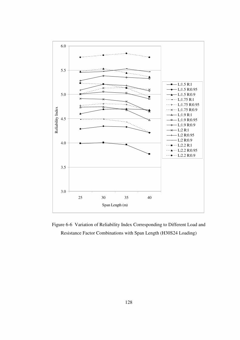
128
3.0
3.5
4.0
4.5
5.0
5.5
6.0
25 30 35 40
Span Length (m)
Rel
iabi
lity
Inde
x
.
L:1.5 R:1L:1.5 R:0.95L:1.5 R:0.9L:1.75 R:1L:1.75 R:0.95L:1.75 R:0.9L:1.9 R:1L:1.9 R:0.95L:1.9 R:0.9L:2 R:1L:2 R:0.95L:2 R:0.9L:2.2 R:1L:2.2 R:0.95L:2.2 R:0.9
Figure 6-6 Variation of Reliability Index Corresponding to Different Load and
Resistance Factor Combinations with Span Length (H30S24 Loading)

129
3.0
3.5
4.0
4.5
5.0
5.5
6.0
25 30 35 40
Span Length (m)
Rel
iabi
lity
Inde
x
.
L:1.5 R:1L:1.5 R:0.95L:1.5 R:0.9L:1.75 R:1L:1.75 R:0.95L:1.75 R:0.9L:1.9 R:1L:1.9 R:0.95L:1.9 R:0.9L:2 R:1L:2 R:0.95L:2 R:0.9L:2.2 R:1L:2.2 R:0.95L:2.2 R:0.9
Figure 6-7 Variation of Reliability Index Corresponding to Different Load and
Resistance Factor Combinations with Span Length (HL93 Loading)
If the target reliability index is chosen as 4.5 considering the maximum current
reliability level of Turkish type prestressed precast concrete bridge girders
using H30S24 load effect with L:1.75 and R:1.0, the following load and
resistance factors may be suggested: L:1.9 and R: 1.0 for designs using
H30S24 loading, and L:1.75 and R:0.9 for designs using HL93 loading.

130
CHAPTER 7
CONCLUSION
7.1 CONCLUDING COMMENTS
The new shift in international bridge design applications is to utilize load and
resistance factor design (LRFD) method that targets a minimum uniform safety
among a variety of bridge designs. LRFD method is calibrated based on study
of series of statistical parameters related to both resistance and load
components. The same reliability theory used in calibration of AASHTO
LRFD is adopted in this research to evaluate the safety levels for Turkish type
precast prestressed bridge girders. These girders are designed to satisfy
minimum requirements of AASHTO LRFD service and strength limit states for
the two truck models, H30S24 and HL93. In this research, different multiple-
girder bridge configurations with variation in span length, type of girders and
number of prestressing strands are studied to investigate the moment due to
loads and flexural resistance at the mid-span. Statistical parameters (probability
distribution, bias factor and coefficient of variation) related to live load,
compressive strength of concrete and tensile strength of prestressing strands are
assessed using the Turkish data. The statistical parameters of other load and
resistance components are taken from the calibration report of AASHTO
LRFD and international research.
131
Based on the results of this research, several conclusions can be drawn:
1. The H30S24 truck model case yields to a conservative design compared
to the HL93 truck model case in terms of safety level evaluation of Turkish
type prestressed precast concrete girders designed in accordance with
AASHTO LRFD. In strength limit state evaluations, the H30S24 loading case
yields to 14% more in terms of reliability index compared to the HL93 loading
case on average. The similar observation is made for the service limit state
with a 10% difference.
2. Reliability indexes determined for the two truck models at service limit
state evaluations are about 20% higher than the ones computed at strength limit
state.
3. For the two truck loadings investigated at strength limit state, reliability
indexes yield to higher values than the target reliability level of 3.5 set in the
AASHTO LRFD. Therefore, the current load and resistance factors (L:1.75
and R:1.0) need not to be modified for design cases in Turkey. If a higher level
of reliability index is targeted in design, design aids provided in this research
can be used. For instance; if the target reliability index is set to be higher than
4.5 considering maximum current reliability level of Turkish type precast
concrete bridge girders, the load and resistance factors may be suggested as;
L:1.9 and R: 1.0 for designs with H30S24 loading, and L:1.75 and R:0.9 for
designs with HL93 loading.
4. Three extrapolation cases described in this research being overall, upper
tail and extreme are used to assess statistical parameters of the live load effect
for an extended period of time using extreme value theory. Out of all these
cases, extreme case is selected to be used in the assessment of time-dependent
live load effects since extreme case is more representative of extreme truck
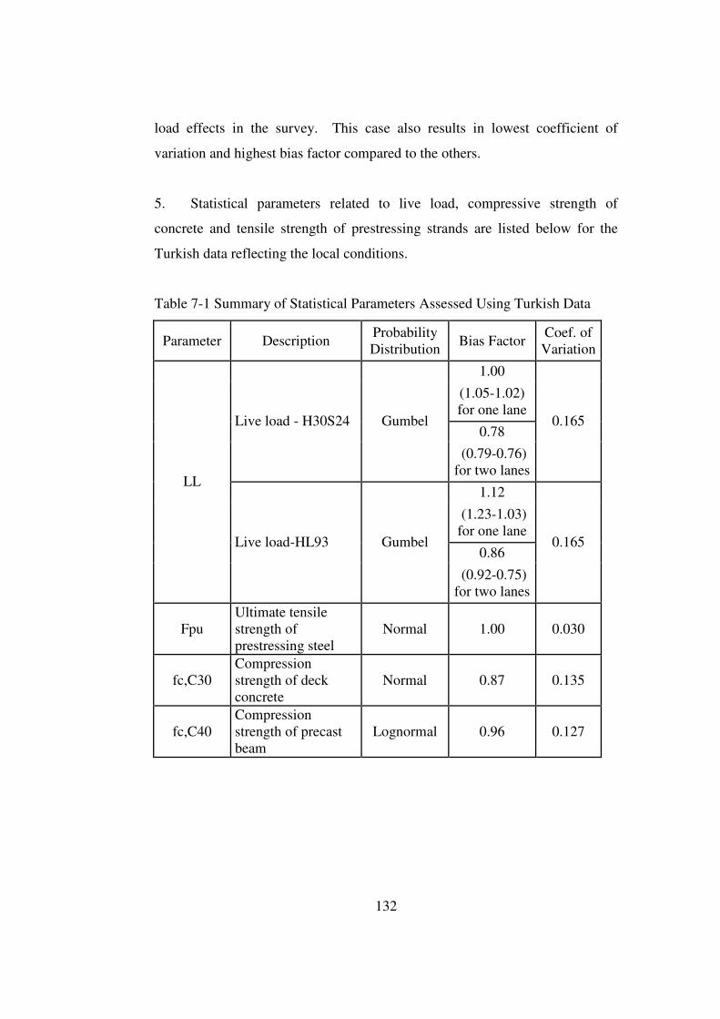
132
load effects in the survey. This case also results in lowest coefficient of
variation and highest bias factor compared to the others.
5. Statistical parameters related to live load, compressive strength of
concrete and tensile strength of prestressing strands are listed below for the
Turkish data reflecting the local conditions.
Table 7-1 Summary of Statistical Parameters Assessed Using Turkish Data
Parameter Description Probability Distribution
Bias Factor Coef. of
Variation
1.00
(1.05-1.02) for one lane
0.78 Live load - H30S24 Gumbel
(0.79-0.76) for two lanes
0.165
1.12
(1.23-1.03) for one lane
0.86
LL
Live load-HL93 Gumbel
(0.92-0.75) for two lanes
0.165
Fpu Ultimate tensile strength of prestressing steel
Normal 1.00 0.030
fc,C30 Compression strength of deck concrete
Normal 0.87 0.135
fc,C40 Compression strength of precast beam
Lognormal 0.96 0.127

133
7.2 RECOMMENDATIONS FOR FUTURE STUDIES
The work presented in this study can be replicated to evaluate the safety levels
for other types of bridges such as steel, post tensioned and reinforced concrete.
The future study can also be carried out to evaluate not only mid-span
moments but also the shear force and negative moments.
In the current study, only bridge girder members are considered. The reliability
level of other components of bridges like piers, supports, abutments and
foundation can be assessed considering the conditions peculiar to Turkey.
In this study, truck catalogs are used to determine the axle spacing of the
surveyed trucks. The distance between each truck axle can be measured to be
reported in the surveys to determine the truck axle load patterns. The General
Directorate of Highways can also classify the trucks during the surveys as
light, medium and heavy weight based on their tonnages.
Other limit states such as extreme event limit state and fatigue limit state
described in the AASHTO LRFD can also be investigated in terms of safety
level evaluations.
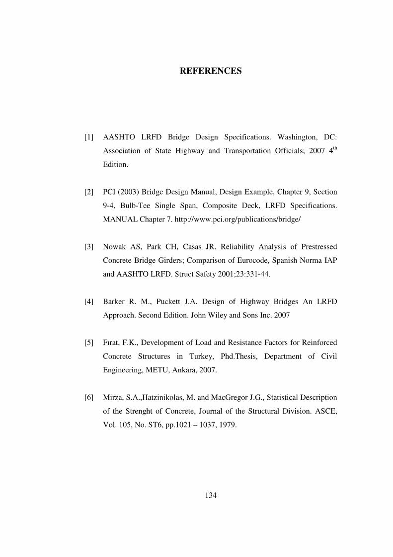
134
REFERENCES
[1] AASHTO LRFD Bridge Design Specifications. Washington, DC:
Association of State Highway and Transportation Officials; 2007 4th
Edition.
[2] PCI (2003) Bridge Design Manual, Design Example, Chapter 9, Section
9-4, Bulb-Tee Single Span, Composite Deck, LRFD Specifications.
MANUAL Chapter 7. http://www.pci.org/publications/bridge/
[3] Nowak AS, Park CH, Casas JR. Reliability Analysis of Prestressed
Concrete Bridge Girders; Comparison of Eurocode, Spanish Norma IAP
and AASHTO LRFD. Struct Safety 2001;23:331-44.
[4] Barker R. M., Puckett J.A. Design of Highway Bridges An LRFD
Approach. Second Edition. John Wiley and Sons Inc. 2007
[5] Fırat, F.K., Development of Load and Resistance Factors for Reinforced
Concrete Structures in Turkey, Phd.Thesis, Department of Civil
Engineering, METU, Ankara, 2007.
[6] Mirza, S.A.,Hatzinikolas, M. and MacGregor J.G., Statistical Description
of the Strenght of Concrete, Journal of the Structural Division. ASCE,
Vol. 105, No. ST6, pp.1021 – 1037, 1979.
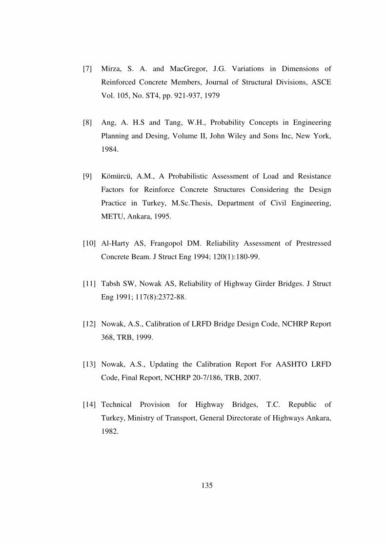
135
[7] Mirza, S. A. and MacGregor, J.G. Variations in Dimensions of
Reinforced Concrete Members, Journal of Structural Divisions, ASCE
Vol. 105, No. ST4, pp. 921-937, 1979
[8] Ang, A. H.S and Tang, W.H., Probability Concepts in Engineering
Planning and Desing, Volume II, John Wiley and Sons Inc, New York,
1984.
[9] Kömürcü, A.M., A Probabilistic Assessment of Load and Resistance
Factors for Reinforce Concrete Structures Considering the Design
Practice in Turkey, M.Sc.Thesis, Department of Civil Engineering,
METU, Ankara, 1995.
[10] Al-Harty AS, Frangopol DM. Reliability Assessment of Prestressed
Concrete Beam. J Struct Eng 1994; 120(1):180-99.
[11] Tabsh SW, Nowak AS, Reliability of Highway Girder Bridges. J Struct
Eng 1991; 117(8):2372-88.
[12] Nowak, A.S., Calibration of LRFD Bridge Design Code, NCHRP Report
368, TRB, 1999.
[13] Nowak, A.S., Updating the Calibration Report For AASHTO LRFD
Code, Final Report, NCHRP 20-7/186, TRB, 2007.
[14] Technical Provision for Highway Bridges, T.C. Republic of
Turkey, Ministry of Transport, General Directorate of Highways Ankara,
1982.

136
[15] Castillo, E. Extreme Value Theory in Engineering, Academic Press Inc.,
1988.
[16] Hwang, E.S., and Nowak, A.S., Simulation of Dynamic Load for
Bridges. ASCE Journal of Structural Engineering, Vol.117, No.5, (1991),
pp. 1413-1434.
[17] J.S. Du , F.T.K. Au. Deterministic and Reliability Analysis of Prestressed
Concrete Bridge Girders: Comparison of the Chinese, Hong Kong and
AASHTO LRFD Codes. Struct Safety Vol. 23, pp 331–344, 2001.
[18] MacGregor, J.G., Mirza, S. A., Ellingwood B. Statistical Analysis of
Resistance of Reinforced and Prestressed Concrete Members. ACI
Journal, No. 80-16, pp. 167-176, 1983.
[19] Mirza SA, Kikuchi DK, MacGregor JG. Flexural Strength Reduction
Factor for Bonded Prestressed Concrete Beams. J ACI 1980;77(4):237–
46.
[20] Ghosn M. and Moses F., Design of Highway Bridges for Extreme
Events, NCHRP Report 489, TRB, 2003.
[21] Szerszen M. M. and Nowak A. S., Calibration of Design Code For
Buildings (ACI 318): Part2-Reliability Analysis and Resistance Factors.
ACI Structural Journal, V100, No.3, May-June 2003.
[22] Eurocode EN 1990, Basis of Structural Design, April 2002.
[23] AASHTO LFD Bridge Design Specifications. Washington, DC:
Association of State highway and Transportation Officials; 1971.

137
[24] Axle Weight Measurements Data Recorded by the General Directorate of
Highways between 1997 and 2006 Years.
[25] Yan-Gang Zhao, Tetsura Ono, A General procedure for first/Second
Order Reliability Method (FORM/SORM), Structural Safety 21 (1999)
95-112.
[26] Hasofer, A. and Lind, N.C., Exact and Invariant Second-Moment Code
Format, Journal of Engineering Mechanics Division, ASCE, Vol. 100,
No. EM. 1, pp. 111-121, 1974.
[27] Breitung, K., Asymptotic Approximation for Multi-normal Integrals,
Journal of Engineering Mechanics Division, ASCE, Vol. 66, No. EM. 3,
pp. 110, 1984.