reliability in the rasch model - kybernetika - · pdf filereliability in the rasch model 317...

K Y B E R N E T I K A — V O L U M E 4 3 ( 2 0 0 7 ) , N U M B E R 3 , P A G E S 3 1 5 – 3 2 6

RELIABILITY IN THE RASCH MODEL

Patrıcia Martinkova and Karel Zvara

This paper deals with the reliability of composite measurement consisting of true-falseitems obeying the Rasch model. A definition of reliability in the Rasch model is proposedand the connection to the classical definition of reliability is shown. As a modification of theclassical estimator Cronbach’s alpha, a new estimator logistic alpha is proposed. Finally,the properties of the new estimator are studied via simulations in the Rasch model.

Keywords: Cronbach’s alpha, Rasch model, reliability

AMS Subject Classification: 62F10, 62P25

1. INTRODUCTION

Let us consider the problem of measuring the reliability of a composite measurementsuch as an educational test. Consider a set of items

Yj = Tj + ej for j = 1, . . . ,m, (1)

where Tj are the unobservable true scores and ej are the error terms with zero meanand a positive variance, independent from the true scores. The observed overallscore is given by Y = Y1 + · · · + Ym and the overall unobservable true score isT = T1 + · · ·+ Tm.

The reliability of such a measurement is defined as the ratio of the variability ofthe true score to the observed variability, that is

Rm = var (T )/var (Y ). (2)

Also, when having two independent measurements Y1 = T + e1, Y2 = T + e2 of thesame property T, where var (e1) = var (e2), the reliability can be expressed as thecorrelation between these two measurements

corr (T + e1, T + e2) =cov (T + e1, T + e2)√

var 2(Y )=

var (T )var (Y )

= Rm. (3)

Since we cannot estimate var (T ), var (e), nor measure the knowledge by the same testtwice and independently, measures to estimate the reliability have been developed.

316 P. MARTINKOVA AND K. ZVARA

A widely used characteristic of reliability is called Cronbach’s alpha. It wasproposed by Cronbach in [6] as a generalization of Kuder–Richardson formula 20 forbinary data (see [9]). Cronbach’s alpha is defined as

αCR =m

m− 1var (Y )−∑

j var (Yj)var (Y )

=m

m− 1

∑∑j 6=k σjk∑∑j,k σjk

, (4)

where σjk is the covariance of the pair (Yj , Yk). A pleasant property of Cronbach’salpha is the fact that this characteristic is easy to estimate from the data simply byusing sample variances and sample covariances instead of their population counter-parts in (4).

Novick and Lewis have shown in [11] that Cronbach’s alpha is always a lowerbound of the reliability and is equal to reliability if, and only if, the test is composedof items that are essentially tau-equivalent, that is if for the items’ true scores itholds simultaneously

var (T1) = · · · = var (Tm) = σ2T

corr (Tj , Tk) = 1, j, k = 1, . . . ,m. (5)

In [13] ten Berge and Zegers came with a series µ0 ≤ µ1 ≤ · · · ≤ Rm of lower boundsto the reliability, where µ0 = αCR is Cronbach’s alpha, and where

µ1 =1∑∑j 6=k σjk

∑∑

j 6=kσjk +

m

m− 1

∑∑

j 6=kσ2jk

1/2

was proposed by Guttman in [8].Connection between Cronbach’s alpha and the intraclass correlation coefficient

(ICC) in terms of the 2-way ANOVA model was investigated in [3]. ICC itself wasdeeply studied in [5], from where this work also takes inspiration.

The nonrobustness of sample estimate αCR is discussed and a robust estimatorof reliability proposed in [14] and more recently in [4].

In this note, we concentrate on the case of educational tests with dichotomouslyscored items. In such a case, the assumptions of the classical model (1) are violated.Therefore, in the next section we propose a new estimate of reliability which shouldbe more appropriate for binary data.

2. ESTIMATION OF RELIABILITY

Interesting findings about Cronbach’s alpha can be made when its sample estimate

αCR =m

m− 1

∑∑j 6=k σjk∑ ∑j,k σjk

(6)

is further rewritten in terms of the two-way ANOVA mixed-effects model: Let ussuppose that the score reached by the ith student in the jth item can be expressedas

Yij = Ai + bj + eij , (7)

Reliability in the Rasch Model 317

where ability of ith person Ai ∼ N(0, σ2A) is a random variable obeying the normal

distribution, bj is an unknown parameter describing the difficulty of jth item andeij ∼ N(0, σ2

e) is a normally distributed error term, independent from abilities Apfor p = 1, . . . , n. In this situation the true score can be expressed as Tij = Ai + bj ,and one can easily see, that conditions (5) of essential tau-equivalence are satisfied,and therefore αCR = Rm. When considering model (7), the sample estimate αCRcan be rewritten as

αCR =MSA −MSe

MSA= 1− 1

FA, (8)

where MSA and MSe are the mean squares and FA is statistic widely used fortesting the hypothesis var (A) = 0, either in a fixed effect model (where also studentabilities are understood as fixed) or in mixed effect model (7), see [10] p. 947. Asan interpretation of (8) we can say, that the greater the estimate of reliability αCRis, the better the educational test can distinguish between the students. Besides,formula (8) can be used for construction of the confidence interval for Cronbach’salpha (see also [7]).

Nevertheless, Feldt in [7] warns, that for a test with dichotomously scored items,the assumptions of analysis of variance are violated. The distribution of error termsmay be far from the normal distribution, and moreover the error term and the truescore cannot be considered independent anymore. Therefore, it is a matter of ques-tion as to what extent at all the classical estimate Cronbach’s alpha (or better saidKuder–Richardson formula 20) is appropriate for tests with dichotomously scoreditems.

The idea of the present contribution (first mentioned in [15]) is to replace theF-statistic in (8) best suited for normally distributed variables by the analogousstatistic appropriate for dichotomous data.

Testing the hypothesis H0 : var (T ) = 0 is equal to testing the submodel B wherethe score Yij depends only on the test item (and does not depend on the student’sability) against the model A + B where the score Yij depends on the student andon the test item. In the fixed-effect model of logistic regression, the appropriatestatistic is the difference of deviances in the submodel and in the model

X2 = D(B)−D(A+B), (9)

where deviance D is defined as a function of the difference of the log-likelihood forthe model and for the saturated model (for details see, e. g. [1], p. 139). Statistic(9) has under the null hypothesis asymptotically (for n fixed and m approachinginfinity) the χ2(n− 1) distribution. Therefore, the proposed estimate is

αlog = 1− n− 1X2

. (10)

In the next sections, we study the properties of the proposed estimate (10), whichwe call logistic alpha, in the Rasch model.


3. RELIABILITY IN THE RASCH MODEL

The model used most often for describing dichotomously scored items (in particularin the context of Item Response Theory) is the logit-normal model, called the Raschmodel (see [12]). In the Rasch model, the probability of correct response yij = 1 orfalse response yij = 0 of person i on item j is given by

P (Yij = yij |Ai) =exp[yij(Ai + bj)]1 + exp(Ai + bj)

, (11)

where Ai ∼ N(0, σ2A) describes the level of ability of person i, and bj is an unknown

parameter describing the difficulty of item j. The conditional distributions areassumed to be independent. Since no error term is assumed in model (11), theclassical definition of reliability (2) is not applicable here.

Inspired by formula (2.3) in [5] we propose to define the reliability of measurementcomposed of binary data obeying the mixed effect model by the ratio

Rm =var [E (Yi|Ai)]

var (Yi). (12)

Similarly to the classical definition, there is the total observed variability in thedenominator, and there is the part of the var (Yi) due to variability of Ai in thenumerator.

For the classical (mixed-effect two-way ANOVA) model, where

E (Y |A) = var (T )

the new definition merges with the classical definition of reliability (2).Formula (12) can be used for defining reliability for binary data obeying any type

of distribution. The formula for the reliability in the Rasch model (11) is following(see the Appendix for detailed derivation):

Rm =

∑mj=1

∑mt=1(Cjt −DjDt)∑m

j=1

∑mt=1(Cjt −DjDt) +

∑mj=1Bj

, (13)

where

Bj = EAeA+bj

(1 + eA+bj )2=

∫ ∞

−∞

eA+bj

(1 + eA+bj )2

1√2πσ2

A

e− A2

2σ2A dA,

Dj = EAeA+bj

1 + eA+bj=

∫ ∞

−∞

eA+bj

1 + eA+bj

1√2πσ2

A

e− A2

2σ2A dA

and

Cjt = EAeA+bj

1 + eA+bj

eA+bt

1 + eA+bt=

∫ ∞

−∞

eA+bj

1 + eA+bj

eA+bt

1 + eA+bt

1√2πσ2

A

e− A2

2σ2A dA.

These integrals cannot be evaluated explicitly, but can be evaluated numerically.Table 1 shows the values of the reliability for some numbers of items L and some


Table 1. Reliability in the Rasch model for different number of items.

Number Variability of abilities σAof items 0.01 0.1 0.2 0.5 0.9 2.5 10

L=3 0.00008 0.00741 0.02881 0.15047 0.34335 0.73121 0.94152

SB R3 0.00008 0.00742 0.02882 0.15054 0.34345 0.73125 0.94153

L=11 0.00028 0.02667 0.09814 0.39386 0.65731 0.90890 0.98335

L=20 0.00050 0.04747 0.16519 0.54160 0.77717 0.94775 0.99077

SB R20 0.00050 0.04746 0.16518 0.54159 0.77716 0.94775 0.99077

L=50 0.00125 0.11078 0.33098 0.74709 0.89711 0.97843 0.99629

SB R50 0.00125 0.11077 0.33095 0.74707 0.89710 0.97843 0.99629

L=100 0.00249 0.19947 0.49735 0.85524 0.94577 0.98910 0.99814

SB R100 0.00249 0.19944 0.49731 0.85522 0.94576 0.98910 0.99814

variabilities of student abilities σA, when the equidistantly distributed item difficul-ties between −0.1 and 0.1 of length L are chosen. The values were calculated usingthe function integrate in software R, using multiple of ±25 of the variability σAas the limits of integration. The maximum absolute error reached in integrationsfor L = 3, L = 11, and L = 20 was less than 0.000025, for L = 50 and L = 100it was less than 0.00013. Table 1 gives an impression that the relationship betweenreliability and number of items follows the Spearman–Brown formula. This formulafor two tests consisting of different numbers (m1 and m2) of tau-equivalent itemshas been proved in the ANOVA model (7) (see [2]) and it says

Rm2 =m2m1Rm1

1 + (m2m1− 1)Rm1

. (14)

Emphasized lines in Table 1 named SB Rm2 are the values Rm2 we would get via theSpearman–Brown formula when setting m1 = 11 and taking the values of the boldline L=11 as Rm1 . The question is, whether the differences are due to integrationerror or not. A theoretical proof for Spearman–Brown formula in the Rasch modelwould be needed to answer the question.

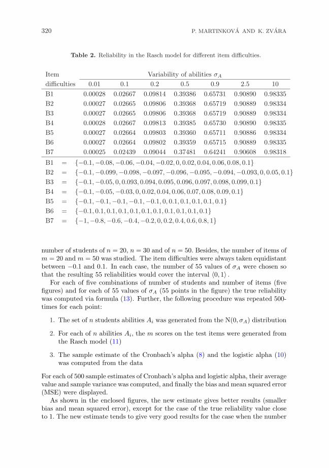
In Table 2 the true reliabilities are displayed for the case of 11 items, when theitem difficulties are unequidistantly distributed with different variability. One cansee that the variability of item difficulties has only a slight impact on test reliabilitywhen compared with impact of the number of items.

4. SIMULATIONS AND A PRACTICAL EXAMPLE

This study was inspired by the data describing 11 dichotomously scored items inbiology. We made, first of all, a simulation study for this case. We studied the


Table 2. Reliability in the Rasch model for different item difficulties.

Item Variability of abilities σAdifficulties 0.01 0.1 0.2 0.5 0.9 2.5 10B1 0.00028 0.02667 0.09814 0.39386 0.65731 0.90890 0.98335B2 0.00027 0.02665 0.09806 0.39368 0.65719 0.90889 0.98334B3 0.00027 0.02665 0.09806 0.39368 0.65719 0.90889 0.98334B4 0.00028 0.02667 0.09813 0.39385 0.65730 0.90890 0.98335B5 0.00027 0.02664 0.09803 0.39360 0.65711 0.90886 0.98334B6 0.00027 0.02664 0.09802 0.39359 0.65715 0.90889 0.98335B7 0.00025 0.02439 0.09044 0.37481 0.64241 0.90608 0.98318

B1 = {−0.1,−0.08,−0.06,−0.04,−0.02, 0, 0.02, 0.04, 0.06, 0.08, 0.1}B2 = {−0.1,−0.099,−0.098,−0.097,−0.096,−0.095,−0.094,−0.093, 0, 0.05, 0.1}B3 = {−0.1,−0.05, 0, 0.093, 0.094, 0.095, 0.096, 0.097, 0.098, 0.099, 0.1}B4 = {−0.1,−0.05,−0.03, 0, 0.02, 0.04, 0.06, 0.07, 0.08, 0.09, 0.1}B5 = {−0.1,−0.1,−0.1,−0.1,−0.1, 0, 0.1, 0.1, 0.1, 0.1, 0.1}B6 = {−0.1, 0.1, 0.1, 0.1, 0.1, 0.1, 0.1, 0.1, 0.1, 0.1, 0.1}B7 = {−1,−0.8,−0.6,−0.4,−0.2, 0, 0.2, 0.4, 0.6, 0.8, 1}

number of students of n = 20, n = 30 and of n = 50. Besides, the number of items ofm = 20 and m = 50 was studied. The item difficulties were always taken equidistantbetween −0.1 and 0.1. In each case, the number of 55 values of σA were chosen sothat the resulting 55 reliabilities would cover the interval 〈0, 1〉 .

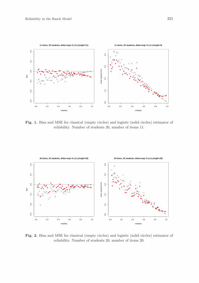
For each of five combinations of number of students and number of items (fivefigures) and for each of 55 values of σA (55 points in the figure) the true reliabilitywas computed via formula (13). Further, the following procedure was repeated 500-times for each point:

1. The set of n students abilities Ai was generated from the N(0, σA) distribution

2. For each of n abilities Ai, the m scores on the test items were generated fromthe Rasch model (11)

3. The sample estimate of the Cronbach’s alpha (8) and the logistic alpha (10)was computed from the data

For each of 500 sample estimates of Cronbach’s alpha and logistic alpha, their averagevalue and sample variance was computed, and finally the bias and mean squared error(MSE) were displayed.

As shown in the enclosed figures, the new estimate gives better results (smallerbias and mean squared error), except for the case of the true reliability value closeto 1. The new estimate tends to give very good results for the case when the number


0.0 0.2 0.4 0.6 0.8 1.0

−0.

3−

0.2

−0.

10.

00.

10.

2

11 items, 20 students, delta=seq(−0.1,0.1,length=11)

reliability

bias

0.0 0.2 0.4 0.6 0.8 1.00.

00.

10.

20.

30.

4


reliability

mea

n sq

uare

d er

ror

Fig. 1. Bias and MSE for classical (empty circles) and logistic (solid circles) estimator of

reliability. Number of students 20, number of items 11.

0.0 0.2 0.4 0.6 0.8 1.0

−0.

3−

0.2

−0.

10.

00.

10.

2


reliability

bias

0.0 0.2 0.4 0.6 0.8 1.0

0.0

0.1

0.2

0.3

0.4

0.5


reliability

mea

n sq

uare

d er

ror




0.0 0.2 0.4 0.6 0.8 1.0

−0.

3−

0.2

−0.

10.

00.

10.

2


reliability

bias

0.0 0.2 0.4 0.6 0.8 1.00.

00.

10.

20.

30.

40.

5


reliability

mea

n sq

uare

d er

ror



0.0 0.2 0.4 0.6 0.8 1.0

−0.

20−

0.15

−0.

10−

0.05

0.00

0.05

0.10


reliability

bias

0.0 0.2 0.4 0.6 0.8 1.0

0.0

0.1

0.2

0.3

0.4

0.5


reliability

mea

n sq

uare

d er

ror




0.0 0.2 0.4 0.6 0.8 1.0

−0.

20−

0.15

−0.

10−

0.05

0.00

0.05

0.10


reliability

bias

0.0 0.2 0.4 0.6 0.8 1.0

0.0

0.1

0.2

0.3

0.4

0.5


reliabilitym

ean

squa

red

erro

r



of items exceeds the number of students (Figure 3). In the case of high number ofstudents in proportion to the number of items (Figure 5), the results of the newestimate are a bit worse.

Let us now look at an example of a real data analysis. We analysed responses oftotal number of 224 students to a biology test composed of 11 dichotomous items.The students were divided into nine groups (nine classes). In Table 3, we can see thenumber of students in each group, the estimate of reliability based on Cronbach’salpha and the estimate of reliability via logistic alpha.

Table 3. Estimation of reliability via Cronbach’s and logistic alpha.

Group # of students αCR αlog

1 21 0.2492918 0.30021227

2 24 −0.1319623 −0.02784881

3 28 0.2562637 0.29611042

4 21 0.4248927 0.47305085

5 31 0.3694124 0.40444782

6 25 0.6944165 0.68331857

7 24 0.2213452 0.26716854

8 23 0.4833022 0.53131265

9 27 0.3570429 0.44172929

In group number 2, both logistic and Cronbach’s alpha gave a negative estimateof reliability. This was caused by small variability of total scores reached by students


in this group. Except one group, the logistic alpha gave always higher estimate ofreliability than the Cronbach’s alpha. This might be an example of underestimationof reliability by Cronbach’s alpha. Nevertheless, the real data examples do not tellus much about which of the two estimates is better, since we do not know the truevalue of the reliability.

5. CONCLUSIONS AND DISCUSSION

While the classical definition of reliability (2) is not appropriate for mixed effectmodels of binary data, we proposed a new definition of reliability (12), which isshown to have the same properties as the classical definition. The new definitionmerges with the classical definition for the classical model (1).

As a counterpart to the classical estimator of reliability Cronbach’s alpha (4),which is based on F-statistics appropriate for continuous data, a new estimate namedlogistic alpha (10), appropriate for binary data, is proposed.

In simulations in the Rasch model, the new estimate gave better results (smallerbias and mean squared error), except for the case of real reliability values close to 1.In particular, the new estimate gave better results for the case of a high number ofitems compared to the number of students. The results of the new estimate tendto be worse for the case of high number of students in proportion to the number ofitems.

Further work should contain a study of the theoretical properties of the newestimate in the case of null hypothesis H0 : Rm = 0 and also in the case when thealternative H1 : Rm > 0 holds. This could lead to improvement of the proposedestimate logistic alpha for true values of reliability close to 1.

APPENDIX: DERIVATION OF THE RELIABILITY IN THE RASCH MODEL

The Rasch model is defined by

P (Yij = 1|Ai) = E (Yij |Ai) =eAi+bj

1 + eAi+bj= pij ,

where Ai ∼ N(0, σ2A) describes the ability of the ith student, i = 1, . . . , n and bj

are fixed unknown parameters describing difficulty of the jth item j = 1, . . . ,m.Therefore the conditional variance is

var (Yij |Ai) = pij(1− pij) =eAi+bj

(1 + eAi+bj )2,

and its mean value is

E var (Yij |Ai) =∫ ∞

−∞

eA+bj

(1 + eA+bj )2

1√2πσ2

A

e− A2

2σ2A dA = Bj .


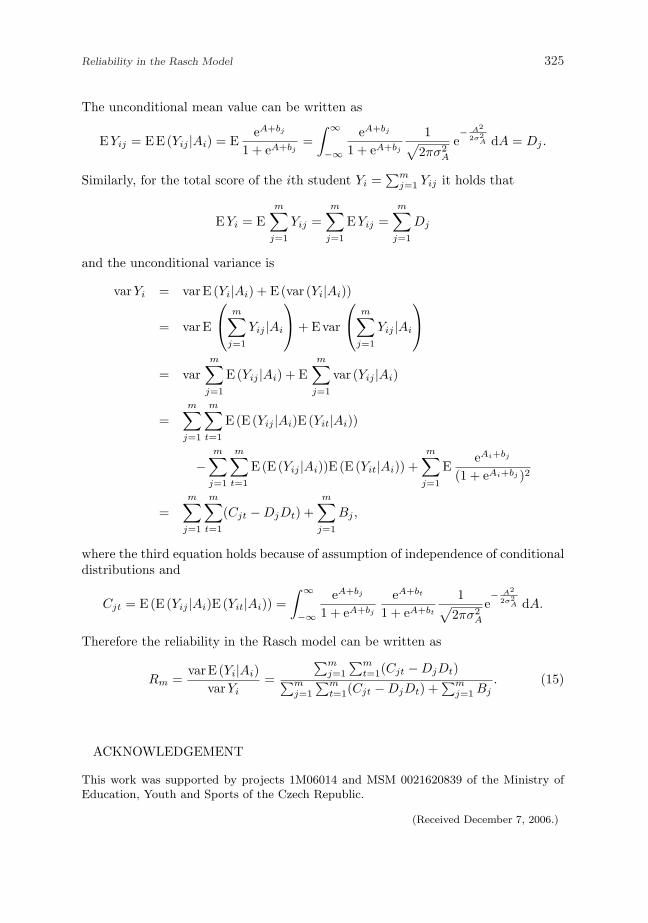
The unconditional mean value can be written as

EYij = E E (Yij |Ai) = EeA+bj

1 + eA+bj=

∫ ∞

−∞

eA+bj

1 + eA+bj

1√2πσ2

A

e− A2

2σ2A dA = Dj .

Similarly, for the total score of the ith student Yi =∑mj=1 Yij it holds that

EYi = Em∑

j=1

Yij =m∑

j=1

EYij =m∑

j=1

Dj

and the unconditional variance is

varYi = var E (Yi|Ai) + E (var (Yi|Ai))

= var E

m∑

j=1

Yij |Ai

+ E var

m∑

j=1

Yij |Ai

= varm∑

j=1

E (Yij |Ai) + Em∑

j=1

var (Yij |Ai)

=m∑

j=1

m∑

t=1

E (E (Yij |Ai)E (Yit|Ai))

−m∑

j=1

m∑

t=1

E (E (Yij |Ai))E (E (Yit|Ai)) +m∑

j=1

EeAi+bj

(1 + eAi+bj )2

=m∑

j=1

m∑

t=1

(Cjt −DjDt) +m∑

j=1

Bj ,

where the third equation holds because of assumption of independence of conditionaldistributions and

Cjt = E (E (Yij |Ai)E (Yit|Ai)) =∫ ∞

−∞

eA+bj

1 + eA+bj

eA+bt

1 + eA+bt

1√2πσ2

A

e− A2

2σ2A dA.

Therefore the reliability in the Rasch model can be written as

Rm =var E (Yi|Ai)

varYi=

∑mj=1

∑mt=1(Cjt −DjDt)∑m

j=1

∑mt=1(Cjt −DjDt) +

∑mj=1Bj

. (15)

ACKNOWLEDGEMENT

This work was supported by projects 1M06014 and MSM 0021620839 of the Ministry ofEducation, Youth and Sports of the Czech Republic.

(Received December 7, 2006.)


R E F E R E N C E S

[1] A. Agresti: Categorical Data Analysis. Wiley, New York 2002.[2] P. D. Allison: A simple proof of the Spearman–Brown formula for continuous test

lengths. Psychometrika 40 (1975), 135–136.[3] G. Bravo and L. Potvin: Estimating the reliability of continuous measures with Cron-

bach’s alpha or the intraclass correlation coefficient: Toward the integration of twotraditions. J. Clin. Epidemiol. 44 (1991), 381–390.

[4] A. Christmann and S. Van Aelst: Robust estimation of Cronbach’s alpha. J. Multi-variate Anal. 97 (2006), 1660–1674.

[5] D. Commenges and H. Jacqmin: The intraclass correlation coefficient distribution-freedefinition and test. Biometrics 50 (1994), 517–526.

[6] L. J. Cronbach: Coefficient alpha and the internal structure of tests. Psychometrika16 (1951), 297–334.

[7] L. S. Feldt: The approximate sampling distribution of Kuder–Richardson reliabilitycoefficient twenty. Psychometrika 30 (1965), 357–370.

[8] L. A. Guttman: A basis for analyzing test-retest reliability. Psychometrika 30 (1945),357–370.

[9] G. Kuder and M. Richardson: The theory of estimation of test reliability. Psychome-trika 2 (1937), 151–160.

[10] J. Neter, W. Wasserman, and M. H. Kutner: Applied Linear Statistical Models.Richard D. Irwin, Homewood, Il. 1985.

[11] M. R. Novick and C. Lewis: Coefficient alpha and the reliability of composite mea-surement. Psychometrika 32 (1967), 1–13.

[12] G. Rasch: Probabilistic Models for Some Intelligence and Attainment Tests. The Dan-ish Institute of Educational Research, Copenhagen 1960.

[13] J. M. F. ten Berge and F. E. Zegers: A series of lower bounds to the reliability of atest. Psychometrika 43 (1978), 575–579.

[14] R. R. Wilcox: Robust generalizations of classical test reliability and Cronbach’s alpha.British J. Math. Statist. Psych. 45 (1992), 239–254.

[15] K. Zvara: Measuring of reliability: Beware of Cronbach. (Merenı reliability aneb bachana Cronbacha, in Czech.) Inform. Bull. Czech Statist. Soc. 12 (2002), 13–20.

Patrıcia Martinkova, Center of Biomedical Informatics, Institute of Computer Science,

Academy of Sciences of the Czech Republic, Pod Vodarenskou vezı 2, 182 07 Praha 8.

Czech Republic.

e-mail: [email protected]

Karel Zvara, Department of Probability and Mathematical Statistics, Faculty of Mathe-

matics and Physics, Charles University in Prague, Sokolovska 83, 186 75 Praha 8. Czech

Republic.

e-mail: [email protected]

reliability in the rasch model - kybernetika - · pdf filereliability in the rasch model 317...

Documents