reliable, low-delay communication in wireless sensor networks
TRANSCRIPT

Degree project in
Reliable, Low-delay Communication in Wireless Sensor Networks
MAHESH BOGADI SHANKAR PRASAD
Stockholm, Sweden, Nov 2011
XR-EE-RT 2011:023
Automatic ControlMaster's thesis

Abstract
Wireless sensor networks consist of tiny computers embedded into an envi-
ronment which can monitor almost anything - such as light, motion, proximity,
temperature, biometrics and chemical substances. Actuators conjoined to sensor
networks can be used not only to sense the environment, but also to interact with
it. Such a design is used to develop automatic control systems, ex. a production
line in a factory. These systems are delay critical and demand high reliability.
Hence wireless sensor networks incorporated into such systems must provide
su�cient reliability as well as low delay communication. However, wireless sen-
sors possess power-constrained radios. Furthermore, wireless communication is
expensive in terms of power consumption. Wireless link conditions are often
harsh, unpredictable and vary considerably in both space, and time. Wireless
sensor networks are formed by multi-hop wireless meshes. Consequently, the
communication in wireless sensor networks lacks the required reliability, and
often exhibits long communication delays.
This Master's thesis investigates about the development of a reliable, and
low end-to-end delay data collection scheme for wireless sensor networks. The
approach is to decrease the number of retransmissions for a packet at the data
link layer in order to decrease the end-to-end delay. However, a decrease in the
number of retransmissions for a packet leads to lower reliability. In order to
compensate for the reliability su�ered, an erasure coding scheme, and a multi-
path routing paradigm are investigated. Accordingly, the thesis focuses on an
implementation, and evaluation of an e�cient combination of fountain coding,
braided multi-path routing, and proportionally fair packet scheduling.
The thesis concludes that fountain coding in combination with braided multi-
path routing and proportionally fair packet scheduling is an e�cient solution
for a wireless sensor network with high loss rates.

Contents
1 Introduction 5
1.1 Problem Statement . . . . . . . . . . . . . . . . . . . . . . . . . . 6
1.2 Method . . . . . . . . . . . . . . . . . . . . . . . . . . . . . . . . 6
1.3 Limitations . . . . . . . . . . . . . . . . . . . . . . . . . . . . . . 7
1.4 Scienti�c Contributions . . . . . . . . . . . . . . . . . . . . . . . 7
1.5 Report Structure . . . . . . . . . . . . . . . . . . . . . . . . . . . 7
2 Background 8
2.1 Wireless Sensor Network (WSN) . . . . . . . . . . . . . . . . . . 8
2.2 Network stack . . . . . . . . . . . . . . . . . . . . . . . . . . . . . 9
2.3 Data-link layer . . . . . . . . . . . . . . . . . . . . . . . . . . . . 10
2.4 Network layer . . . . . . . . . . . . . . . . . . . . . . . . . . . . 10
2.4.1 Routing in WSN . . . . . . . . . . . . . . . . . . . . . . . 11
2.4.2 Multi-path routing . . . . . . . . . . . . . . . . . . . . . 12
2.4.3 Proportionally fair packet scheduling . . . . . . . . . . . . 15
2.5 Transport layer . . . . . . . . . . . . . . . . . . . . . . . . . . . 16
2.5.1 Fountain codes . . . . . . . . . . . . . . . . . . . . . . . . 17
2.6 Contiki operating system . . . . . . . . . . . . . . . . . . . . . . 18
2.6.1 Rime . . . . . . . . . . . . . . . . . . . . . . . . . . . . . . 18
2.6.2 Contiki collect . . . . . . . . . . . . . . . . . . . . . . . . 19
2.6.3 Neighbor discovery . . . . . . . . . . . . . . . . . . . . . . 19
2.6.4 Contiki MAC . . . . . . . . . . . . . . . . . . . . . . . . . 19
3 Design and
Implementation 20
3.1 System design . . . . . . . . . . . . . . . . . . . . . . . . . . . . . 20
3.2 Contiki collect . . . . . . . . . . . . . . . . . . . . . . . . . . . . 23
3.3 Fountain coding . . . . . . . . . . . . . . . . . . . . . . . . . . . 24
3.3.1 Encoding . . . . . . . . . . . . . . . . . . . . . . . . . . . 25
3.3.2 Decoding . . . . . . . . . . . . . . . . . . . . . . . . . . . 26

3.3.3 Variation . . . . . . . . . . . . . . . . . . . . . . . . . . . 26
3.4 Braided multi-path
routing . . . . . . . . . . . . . . . . . . . . . . . . . . . . . . . . . 27
3.5 Proportionally fair
packet scheduling . . . . . . . . . . . . . . . . . . . . . . . . . . . 28
3.6 Design choices
and alternatives . . . . . . . . . . . . . . . . . . . . . . . . . . . . 29
4 Evaluation 30
4.1 Experiments . . . . . . . . . . . . . . . . . . . . . . . . . . . . . . 30
4.2 Network topology . . . . . . . . . . . . . . . . . . . . . . . . . . . 31
4.3 Reliability . . . . . . . . . . . . . . . . . . . . . . . . . . . . . . . 31
4.4 Retransmissions . . . . . . . . . . . . . . . . . . . . . . . . . . . . 32
4.5 End-to-end delay . . . . . . . . . . . . . . . . . . . . . . . . . . . 33
4.6 Power consumption . . . . . . . . . . . . . . . . . . . . . . . . . . 34
4.7 Summary . . . . . . . . . . . . . . . . . . . . . . . . . . . . . . . 35
5 Conclusions and future work 36
Bibliography 37
6 Appendix 40
6.1 Reliability . . . . . . . . . . . . . . . . . . . . . . . . . . . . . . . 40
6.1.1 Summary graph about reliability . . . . . . . . . . . . . . 45
6.2 Retransmissions . . . . . . . . . . . . . . . . . . . . . . . . . . . . 45
6.2.1 Summary graph about retransmissions . . . . . . . . . . 50
6.3 End-to-end delay . . . . . . . . . . . . . . . . . . . . . . . . . . . 50
6.3.1 End-to-end delay distribution . . . . . . . . . . . . . . . 58
6.3.2 Minimum and maximum end-to-end delay . . . . . . . . . 63
6.3.3 Summary graph about end-to-end delay . . . . . . . . . . 68
6.4 Power consumption . . . . . . . . . . . . . . . . . . . . . . . . . . 68

List of Tables
4.1 Experiments for the evaluation . . . . . . . . . . . . . . . . . . . 30
4

List of Figures
2.1 Network stack . . . . . . . . . . . . . . . . . . . . . . . . . . . . . 9
2.2 Collection Tree . . . . . . . . . . . . . . . . . . . . . . . . . . . . 12
2.3 Braided multi-path routing . . . . . . . . . . . . . . . . . . . . . 15
2.4 Proportionally fair packet scheduling . . . . . . . . . . . . . . . . 16
2.5 Neighbor discovery . . . . . . . . . . . . . . . . . . . . . . . . . . 19
3.1 System design of the nodes . . . . . . . . . . . . . . . . . . . . . 21
3.2 System design of the sink . . . . . . . . . . . . . . . . . . . . . . 22
3.3 Contiki Collect . . . . . . . . . . . . . . . . . . . . . . . . . . . . 23
3.4 Overview of fountain coding . . . . . . . . . . . . . . . . . . . . . 24
3.5 Encoding and decoding of fountain coding . . . . . . . . . . . . . 25
3.6 The series of packets . . . . . . . . . . . . . . . . . . . . . . . . . 26
3.7 Fountain coding for two packets . . . . . . . . . . . . . . . . . . . 27
3.8 Braided multi-path routing . . . . . . . . . . . . . . . . . . . . . 28
3.9 Proportionally fair packet scheduling . . . . . . . . . . . . . . . . 29
4.1 Network topology . . . . . . . . . . . . . . . . . . . . . . . . . . . 31
4.2 Reliability at di�erent transmission and reception success rates . 32
4.3 Maximum retransmissions at di�erent transmission and reception
success rates . . . . . . . . . . . . . . . . . . . . . . . . . . . . . . 33
4.4 Average end-to-end delay at di�erent transmission and reception
success rates . . . . . . . . . . . . . . . . . . . . . . . . . . . . . . 34
4.5 Power consumption at 60% transmission and reception success rate 35
6.1 Reliability per node 60% transmission and reception success rate 40
6.2 Reliability per node 65% transmission and reception success rate 41
6.3 Reliability per node 70% transmission and reception success rate 41
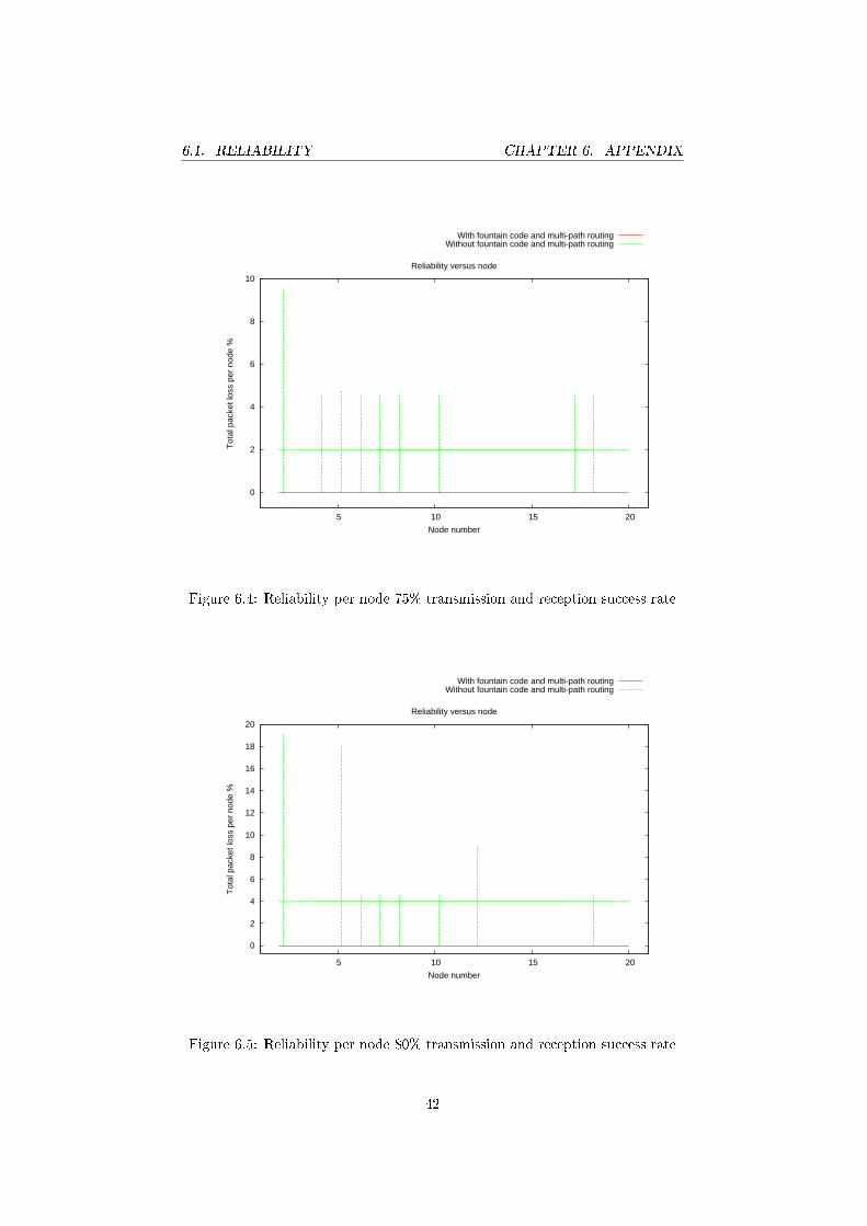
6.4 Reliability per node 75% transmission and reception success rate 42
6.5 Reliability per node 80% transmission and reception success rate 42
6.6 Reliability per node 85% transmission and reception success rate 43
6.7 Reliability per node 90% transmission and reception success rate 43
5

6.8 Reliability per node 95% transmission and reception success rate 44
6.9 Reliability at di�erent transmission and reception success rates . 45
6.10 Retransmissions 60% transmission and reception success rate . . 46
6.11 Retransmissions 65% transmission and reception success rate . . 46
6.12 Retransmissions 70% transmission and reception success rate . . 47
6.13 Retransmissions 75% transmission and reception success rate . . 47
6.14 Retransmissions 80% transmission and reception success rate . . 48
6.15 Retransmissions 85% transmission and reception success rate . . 48
6.16 Retransmissions 95% transmission and reception success rate . . 49
6.17 Retransmissions 95% transmission and reception success rate . . 49
6.18 Maximum retransmissions at di�erent transmission and reception
success rates . . . . . . . . . . . . . . . . . . . . . . . . . . . . . . 50
6.19 Average end-to-end delay per node at 60% transmission and re-
ception success rate . . . . . . . . . . . . . . . . . . . . . . . . . . 51
6.20 Average end-to-end delay per node at 65% transmission and re-
ception success rate . . . . . . . . . . . . . . . . . . . . . . . . . . 52
6.21 Average end-to-end delay per node at 70% transmission and re-
ception success rate . . . . . . . . . . . . . . . . . . . . . . . . . . 53
6.22 Average end-to-end delay per node at 75% transmission and re-
ception success rate . . . . . . . . . . . . . . . . . . . . . . . . . . 54
6.23 Average end-to-end delay per node at 80% transmission and re-
ception success rate . . . . . . . . . . . . . . . . . . . . . . . . . . 55
6.24 Average end-to-end delay per node at 85% transmission and re-
ception success rate . . . . . . . . . . . . . . . . . . . . . . . . . . 56
6.25 Average end-to-end delay per node at 90% transmission and re-
ception success rate . . . . . . . . . . . . . . . . . . . . . . . . . . 57
6.26 Average end-to-end delay per node at 95% transmission and re-
ception success rate . . . . . . . . . . . . . . . . . . . . . . . . . . 58
6.27 Delay distribution 60% transmission and reception success rate . 59
6.28 Delay distribution 65% transmission and reception success rate . 59
6.29 Delay distribution 70% transmission and reception success rate . 60
6.30 Delay distribution 75% transmission and reception success rate . 60
6.31 Delay distribution 80% transmission and reception success rate . 61
6.32 Delay distribution 85% transmission and reception success rate . 61
6.33 Delay distribution 90% transmission and reception success rate . 62
6.34 Delay distribution 95% transmission and reception success rate . 62
6.35 Delay range at 60% transmission and reception success rate . . . 63
6.36 Delay range at 65% transmission and reception success rate . . . 64
6.37 Delay range at 70% transmission and reception success rate . . . 64
6.38 Delay range at 75% transmission and reception success rate . . . 65

6.39 Delay range at 80% transmission and reception success rate . . . 65
6.40 Delay range at 85% transmission and reception success rate . . . 66
6.41 Delay range at 90% transmission and reception success rate . . . 66
6.42 Delay range at 95% transmission and reception success rate . . . 67
6.43 Average end-to-end delay at di�erent transmission and reception
success rates . . . . . . . . . . . . . . . . . . . . . . . . . . . . . . 68
6.44 Power consumption at 60% transmission and reception success rate 69
6.45 Power consumption at 65% transmission and reception success rate 69
6.46 Power consumption at 70% transmission and reception success rate 70
6.47 Power consumption at 75% transmission and reception success rate 70
6.48 Power consumption at 80% transmission and reception success rate 71
6.49 Power consumption at 85% transmission and reception success rate 71
6.50 Power consumption at 90% transmission and reception success rate 72
6.51 Power consumption at 95% transmission and reception success rate 72

Chapter 1
Introduction
Wireless Sensor Networks (WSN) consist of tiny computers embedded into the
environment that can monitor almost anything - such as light, motion, proxim-
ity, temperature, biometrics and chemical substances. It has become a vision to
deploy sensor networks not only to sense the environment, but also to interact
with it, by means of networked actuators conjoined to the networked sensors.
Many such WSNs require de�nite reliability, and delay guarantees.
In order to provide high reliability and low delay, this thesis mainly explores
incorporation of fountain codes and multi-path routing into WSNs. Fountain
coding is a type of network coding. It is used to transfer broadcast or multi-cast
data reliably[1]. Multi-path routing brings path-redundancy into the network
and increases reliability in WSNs. Some of the multi-path routings are proven
to be energy e�cient, adaptive to topology changes, and disseminates the net-
work load well [2].
Fountain coding is an an e�cient erasure coding scheme[3], in which the
transmitter disperses coded fragments towards the receiver [1]. Once the re-
ceiver has received any N fragments in any order, where N is greater than the
original number of data fragments, the whole data can be recovered. Incorpo-
ration of this coding scheme increases reliability by sending redundant encoded
packets. The computational costs of the fountain codes are small, scaling lin-
early with the number of data fragments [1].
Multi-path routing constructs multiple paths for the transmission of sensor
information in order to increase redundancy. Thus, it increases the probabil-
ity of successful packet delivery to the sink [2]. In large sensor networks, it
also mitigates network congestion. Thus it may reduce the end-to-end delay
5

1.1. PROBLEM STATEMENT CHAPTER 1. INTRODUCTION
[2]. It conserves energy, and enables spectrum reuse[2]. In braided multi-path
routing, there is a primary path that is mainly used for routing, and several
alternate braided paths are maintained [2]. Braided paths may share nodes. In
other words, node disjointedness (no node is present in multiple paths) is not a
requirement. Braided multi-path routing is an e�cient localized enforcement-
based scheme for collection tree [2]. Proportionally fair scheduling improves the
multi-path routing [4]. It dynamically determines the number of packets to be
sent to the parent nodes (primary and secondary) of the multi-path, inversely
proportional to the routing metric of the parents. [4].
1.1 Problem Statement
A wireless sensor network comprises of wireless sensors as its nodes. The
wireless sensors possess power-constrained radios. They are networked by form-
ing multi-hop wireless meshes. Furthermore, wireless communication is expen-
sive in terms of power consumption. Also, wireless link conditions are often
harsh, unpredictable and vary considerably in both space, and time. Conse-
quently, the communication in wireless sensor networks lacks the required reli-
ability. In addition, it often exhibits long communication delays. This does not
be�t for applications such as a production line in a factory, which requires reli-
able, and e�cient control. Hence, there is a need for a solution which provides
low delay as well as high reliability.
1.2 Method
The method used in the thesis is that of experimentation [5]. I implemented
a fountain coding scheme and a braided multi-path with proportionally fair
packet scheduling combination as a proposed solution to enhance reliability and
reduce end-to-end delay. Then I ran the experiments (with and without the
solution) with di�erent packet transmission and reception success rates using
the Cooja network simulator[6]. I measured reliability (percentage of the total
packet loss), end-to-end delay (average time taken by a packet to reach the sink
from a source), maximum link-to-link retransmissions (average of maximum
data-link layer retransmissions su�ered by a packet whilst traveling from the
source to the sink) and power consumption of each node. Priorly, I had studied
wireless sensor network architecture[7], reprogramming wireless sensor networks
on Contiki platform, network coding, multi-path routing techniques and Cooja
6

1.3. LIMITATIONS CHAPTER 1. INTRODUCTION
simulator [6]. The results from the experiments are plotted as graphs using
gnuplot [8]and compared. This comparative analysis is used in the evaluation
of the results and is the basis for the conclusion of the thesis.
1.3 Limitations
Energy e�ciency is one of the prominent considerations in designing a WSN.
But, the thesis does not design the solution with respect to energy e�ciency.
However, the e�orts of the thesis to reduce number of retransmissions at the
link layer, and the usage of a braided multi-path routing have been proven to be
energy e�cient. The thesis does not explore the other considerations of WSNs,
such as mobility, multi-sink, etc.
1.4 Scienti�c Contributions
WSNs are formed by multi-hop wireless meshes. Consequently, the com-
munication in wireless sensor networks lacks the required reliability, and often
exhibits long communication delays. The thesis contributes mainly at providing
a WSN with de�nite delay and reliability guarantees. This is the �rst known
e�ort about evaluating fountain coding in WSN, with combination of braided
multi-path, and proportionally fair packet scheduling. The thesis shows promis-
ing results regarding reliability, and low-delay that can be achieved by using
fountain coding and multi-path routing in a WSN. In short, the scienti�c con-
tribution of the thesis is a solution towards building a robust WSN with respect
to reliability and low-delay.
1.5 Report Structure
The layout of the succeeding parts of this report is as follows. In the next
chapter, the background studies are summarized. The design, and implementa-
tion details are covered in the consecutive chapter, followed by the chapter on
evaluation of the results. The last chapter provides the conclusion of the thesis
study, and the future works that can be performed using it as a basis.
7

Chapter 2
Background
This chapter introduces the required background to the thesis. The thesis
requires background knowledge of WSN architecture, network stack for WSN,
collection tree paradigm, reliability factors in WSN, delay factors in WSN, net-
work coding, multi-path routing, packet scheduling, and the Contiki operating
system.
2.1 Wireless Sensor Network (WSN)
A WSN consists of tiny sensing computers called sensor nodes[7]. These sen-
sors communicate through radio communication (wireless) to form a network.
WSNs can monitor by sensing almost anything - such as light, motion, prox-
imity, temperature, biometrics and chemical substances. Actuators are devices,
such as valves or switches, that perform actions such as turning things on or o�
or making adjustments in an operational system. Actuators conjoined to sensor
networks can be used not only to sense the environment, but also to interact
with it. Such a design is used to develop automatic control systems, ex. a pro-
duction line in a factory [9]. These systems are delay critical and demand high
reliability. Hence wireless sensor networks incorporated into such systems must
provide su�cient reliability as well as low delay communication.
However, wireless sensors possess power-constrained radios. Furthermore,
wireless communication is expensive in terms of power consumption. Wireless
link conditions are often harsh, unpredictable and vary considerably in both
space and time. Wireless sensor networks are formed by multi-hop wireless
meshes. Consequently, the communication in wireless sensor networks lacks the
required reliability, and often exhibits long communication delays.
8

2.2. NETWORK STACK CHAPTER 2. BACKGROUND
2.2 Network stack
The unpredictable wireless link conditions and resource constrains cause adver-
sity in ensuring reliability in WSNs. The wireless communication between the
sensor nodes is often prone to errors which can degrade the overall quality of a
network. In addition, the multi-hop communication in WSNs ampli�es the unre-
liability of data transmissions to the sink. Ensuring the required low delay along
with su�cient reliability compounds the problem. Hence, an e�cient commu-
nication providing low delay and reliability in a WSN depends on the link-level
transmissions between sensor nodes [10], and the end-to-end transmissions from
sensors to the sink. The sensor to sensor or the node to node communication
is ensured and controlled at the data link layer of the network stack, where as,
end-to-end communication is facilitated by the network as well as the transport
layers [11]. Therefore, the thesis explores the data-link, network, and transport
layers of WSNs from the perspective of increasing reliability and lowering delay.
This section briefs the background about di�erent layers of the network stack
of a WSN.
Figure 2.1: Network stack
9

2.3. DATA-LINK LAYER CHAPTER 2. BACKGROUND
2.3 Data-link layer
The data-link layer is responsible for reliability of the packet transfer from one
sensor node to another in a multi-hop data-path from the source to the sink in a
WSN. Retransmissions between two nodes are used to achieve reliability at the
data-link layer. Traditionally, a sensor node in a WSN transmits a data frame
to the next neighbor node on the data path, and waits for an acknowledgment
for that frame. If the acknowledgement does not arrive within a give timeout
period, the node retransmits the frame. The node retries to send the frame to
the neighbor node until it receives an acknowledgement for the frame, or the
maximum number of allowed retries is reached. However, retransmissions have
drawbacks too. In some cases, they increase delay, cause congestion and clog
bu�ers of the network nodes. Hence, decreasing the number of retransmissions
mitigates delay, congestion and bu�er usage concerns. It also conserves energy.
The number of retransmissions allowed at the data-link layer may be con�gured
to a lower value, when other reliability measures such as redundant data trans-
mission, error correcting or/and data encoding techniques are incorporated into
the system.
2.4 Network layer
The network layer is responsible for determining routes from every sensor node
to the sink in a WSN for end-to-end delivery of sensor data. The routes tra-
versed by the packets from the sensors to the sink are computed, and established
by network layer routing algorithms. Routing in WSNs is very di�erent from
normal networks, because of the unique qualities and limitations of WSNs. The
unpredictable wireless link dynamics causes the topology of WSNs to change
continuously and erratically [11]. This necessitates that data �ow routes in a
WSN to be formed dynamically in order to provide reliable data delivery in
WSNs. Hence, reliability should also be guaranteed at this layer in terms of
dynamic route determination and management [11].
The routing scheme in a WSN plays a vital role regarding reliability, and
delay of the end-to-end data transmission. An e�cient routing in a network
leads to smart distribution of the tra�c across the network. However, several
e�cient routing paradigms such as OSPF, require each node to gather infor-
mation of the whole network topology, which can lead to high delay in network
topology convergence and signi�cant amount of routing data exchange. Such
a routing paradigm is not suited for a WSN. Therefore, a WSN necessitates
10

2.4. NETWORK LAYER CHAPTER 2. BACKGROUND
a routing method which can use localized information which avoids delay in
topology convergence and routing data exchange expenses[11].
Routing in a WSN involves two basic activities :
� Path determination - determining and designating routes from a source to
the sink.
� Packet switching - transporting packets through designated routes [11].
2.4.1 Routing in WSN
Routing protocols in a WSN use metrics to evaluate the best paths for a packet
to travel from a source to the sink. A routing metric is a standard of measure-
ment, such as path bandwidth, that is used by routing algorithms to determine
the best path to a destination. The metric value of a route indicates the proxim-
ity of the node to the sink or the total cost of all links in a path from the node to
the sink. Expected transmission count (ETX) metric is a metric for multi-hop
wireless networks [12]. Route selection using ETX accounts for link loss ratios,
the asymmetry of the loss ratios in the two directions of each link, and the reduc-
tion of throughput due to interference among the successive hops of a route [12].
A basic notion for path determination at a node is to �nd routes with lowest
metric values from the node to the sink. These routes or shortest paths de�ne
a connectivity graph (a tree) describing which nodes can communicate directly
over a single hop. However, generally, WSNs are data-gathering networks in-
volving a many-to-one communication model. Hence, in WSNs routes tra�c for
the data are not bidirectional, they are unidirectional towards the sink. Thus
the graph formed by the routes is a directed tree with the sink as its root. This
tree based routing is also known as collection tree.
WSNs are multi-hop wireless meshes. Wireless communication links found
in WSNs are prone to signi�cant loss rates, and the loss rate varies dynamically
with environmental factors. Routing protocols must take into account such un-
derlying factors. Hence it must encompass connectivity analysis, neighborhood
management with limited storage, and routing on dense WSNs with simple,
low-power radios.
11

2.4. NETWORK LAYER CHAPTER 2. BACKGROUND
Figure 2.2: Collection Tree
For these reasons, the design goals for a routing protocol in WSN include
selection of reliable and low-delay routes, simplicity, low operational overhead,
robustness and stability in the face of unusual and unforeseen circumstances,
rapid convergence or agreement on routes, and �exibility in quickly and accu-
rately adapting to a wide variety of network circumstances. In addition, WSNs
cannot a�ord to abstract all the details of lower-layer protocols and, thus, mo-
tivate cross-layer design and optimizations in routing. These factors motivate
di�erentiated approaches to routing in WSNs.
2.4.2 Multi-path routing
Reliability of a route in a WSN established by a routing protocol may decrease
because of the wireless link conditions, network congestion and energy deple-
tion at the sensor nodes. In such a scenario, an obvious approach to better the
reliability is through redundancy. Multiple copies of a packet is sent through
a single path, which increases the probability that the sink receives the packet.
However, such a single path approach does not address issues such as node fail-
ure, congestion, issues with topology changes and long delays. In certain cases,
a single path approach may worsen the network with several negative e�ects,
12

2.4. NETWORK LAYER CHAPTER 2. BACKGROUND
such as increase in congestion, heavy usage of certain paths and fast depletion
of energy of the nodes in those paths, and thus resulting in low reliability. In
order to address these negative e�ects, routing solutions based on a multi-path
approach are put forth for WSNs [11].
Multi-path routing determines and assigns multiple routes from a given sen-
sor node to the sink. The transmission of data among the multi-path brings
path redundancy and increased reliability by ampli�cation of the probability of
the sink successfully receiving the data through anyone of the multiple paths.
Multi-path routing decreases network congestion, provides proof against node
failures and helps to distribute and share network tra�c among multiple paths
which may avoid heavy usage of certain paths, hence nodes. Multi-path routing
is apt when redundant data transmission is used to increase reliability.
The two important metrics in evaluating the performance of a multi-path
routing scheme are resilience and maintenance overhead. There is an inherent
trade-o� between these two quantities. Becoming more resilient typically con-
sumes more energy, and incurs more maintenance overhead. Typically, multi-
path routing has been deployed for two reasons: load balancing and robustness.
Load-balancing is essential to conserve energy in sensor networks[2].
There are two types of paths generally constructed in multi-path routing:
� A primary path which is the most optimal path with least cost or metric
from a node to the sink.
� A set of alternate paths. An alternate path is a sub-optimal path with
cost or metric slightly higher than the primary path.
A desirable goal in multi-path routing is to deliver data along the primary (best
available) path. However, for a scalable recovery from failure of the primary
path as well as distributing the load, a small number of alternative paths are
constructed. Maintaining the alternate paths must incur low computational
overhead and memory. Also it is demonstrated that multi-path routing can be
used for energy e�cient recovery from failure in wireless sensor networks [2].
The multi-paths classi�ed generally into two types based on the exclusivity
of the nodes among the alternate paths :
� Disjointed multi-paths - These multi-path do not share any node among
di�erent paths. Thus the paths are disjointed by nodes of the network.
13

2.4. NETWORK LAYER CHAPTER 2. BACKGROUND
In this formation failure of one path does not a�ect the performance of
the other paths. However, it results in increase in the overall latency of
the alternate paths. Moreover, in order to establish disjointed paths, each
node of the network needs to be aware of the whole topology of network or
the information about the other paths, which brings the issues of routing
convergence and routing data exchange expenses. Therefore, disjointed
multi-paths are computational expensive to construct and maintain with-
out providing signi�cant bene�ts of reliability and delay [2].
� Braided multi-paths - In this case, paths may have overlapping portions
and hence can share nodes. As a result, all the paths are not indepen-
dent of each other which facilitates usage of mere localized information
to construct routing information base, which results in faster convergence
and lesser routing data exchange [2]. Generally the alternate paths over-
lap the portions of the primary path. Hence, it appears as if the alternate
paths are braided around the primary path. Thus, the latency incurred by
the alternate paths may be lower than the alternate paths constructed in
disjointed multi-paths. Disjoint multi-path and braided multi-path have
similar patterned failure resilience. However the braided multi-paths have
higher resilience to isolated failures and lesser overhead for maintenance
of alternate paths. Also braided multi-path is more energy e�cient [2].
14

2.4. NETWORK LAYER CHAPTER 2. BACKGROUND
Figure 2.3: Braided multi-path routing
2.4.3 Proportionally fair packet scheduling
This section investigates scheduling techniques appropriate for multi-path
routing. A compromise-based solution is required in order to maintain a balance
among con�icting, and competing interests. For example, in order to increase
reliability of end to end data transmission in a WSN, one may think about
sending certain packets on non-shortest paths. Similarly, in order to reduce
network congestion of routing paths, one may o�oad the data tra�c to other
high-cost paths. Proportionally fair packet scheduling is a compromise-based
algorithm. It tries to maximize total wireless network throughput at the cost of
scheduling packets onto sub-optimal paths. This is done by assigning each data
path a scheduling priority (depending on the implementation) that is inversely
15

2.5. TRANSPORT LAYER CHAPTER 2. BACKGROUND
Figure 2.4: Proportionally fair packet scheduling
proportional to its anticipated resource consumption [4].
Weighted fair queuing (WFQ) is used to achieve proportionally fair schedul-
ing. The scheduling weights for data paths i are set to wi = 1 / ci, where the
cost ci is the amount of consumed resources. In case of WSN, the cost ci can
be the routing metric of the path. In other words, lesser number of packets are
scheduled onto paths with higher routing metric [13].
2.5 Transport layer
The objective of transport layer protocols is to provide reliability and QoS
services for data transfer over inherently unreliable, and resource-constrained
WSNs. The following are the interrelated guarantees and services that may be
needed in WSNs at this layer [14]:
� Reliable delivery guarantee - It should ensure that the data arrive from
origin to destination without loss.
� Priority delivery - The data generated within the WSN may be of di�er-
ent priorities; e.g., the data corresponding to an unusual event detection
may have much higher priority than periodic background readings. If the
network is congested, it is important to ensure that at least the high pri-
ority data get through, even if the low-priority data have to be dropped
or suppressed.
16

2.5. TRANSPORT LAYER CHAPTER 2. BACKGROUND
� Delay guarantee - In time-critical applications, particularly those where
the sensor data are used to initiate some form of actuation or response,
the data packets generated by sensor sources may have strict requirements
for delivery to the destination within a speci�ed time.
� Energy-e�cient delivery - Energy wastage during times of network con-
gestion must be minimized, for instance by forcing any necessary packet
drops to occur as close to the source as possible.
� Fairness - Depending on the nature of the application, varying notions
of fairness may be relevant. These notions range from ensuring that all
nodes in the network provide equal amounts of data (e.g. in a simple data-
gathering application), to max�min fairness, to proportional fairness.
� Application-speci�c, data-centric quality of service - In general, given the
bandwidth/energy resource constraints, a data-centric QoS goal requires
that the network as a whole provides a picture of the sensed environment
as accurate as possible.
The thesis concentrates on providing certain reliable delivery guarantee, delay
guarantee, and fairness in a WSN. Therefore, it investigates on fountain coding,
and redundant packet transmission.
2.5.1 Fountain codes
Fountain codes are a type of network codes. Fountain codes are sparse-graph
erasure codes. Erasure code is a forward error correction code [3]. They are
suitable for communications with data loss and unreliable data channels, such
as a WSN. Typically in a WSN, the receiver (the sink) is not aware of the pres-
ence of the sender. Nor does it send any acknowledgment back to the sender
notifying that the data is being received fully as well as correctly. Traditional
approach to provide su�cient reliability from data loss in WSN is to simply
transmit each packet multiple times, anticipating that one of them will reach
the receiver. In contrast, fountain codes make encoded packets that are random
functions of a set of packets (data units). The transmitter sprays packets at the
receiver without concerning about which packets may be successfully received.
Once the receiver has received any N packets, where N is just slightly greater
than the original number of packets sent K, all the packets in the set can be
recovered. The encoded packets need not be received or sent in any order. The
computational costs of the best fountain codes are small and they scale linearly
17

2.6. CONTIKI OPERATING SYSTEM CHAPTER 2. BACKGROUND
with the number of packets in the set.
As D. J. C. MacKay describes in his paper [1]:-
The encoder of a fountain code is a metaphorical fountain that pro-
duces an endless supply of water drops (encoded packets); let us say
the original source �le has a size of Kl bits, and each drop contains
l encoded bits. Now, anyone who wishes to receive the encoded �le
holds a bucket under the fountain and collects drops until the num-
ber of drops in the bucket is a little larger than K. They can then
recover the original �le.
Fountain codes are rateless. In rateless codes, the number of encoded packets
that can be generated from the plain data is potentially in�nite. Hence, one
can increase or decrease the number of encoded packets sent, depending upon
the degree of reliability required and/or the degree of erasure. In other words,
if one can calculate how lossy the communication is, then the number of en-
coded packets to be generated and sprayed at the receiver can be determined.
If the link dynamics of the channel changes constantly and unpredictably, the
determination of the number of encoded packets to be sent can be performed
dynamically, and adaptively. This �exibility makes fountain codes an apt choice
for a WSN.
2.6 Contiki operating system
Contiki is an open source multi-tasking operating system[15]. It is designed
for memory-e�cient networked embedded systems and wireless sensor networks
[15]. Contiki has been used is a variety of projects, such as road tunnel �re mon-
itoring, intrusion detection, wildlife monitoring, and in surveillance networks
[15]. Contiki contains two communication stacks, namely uIP and Rime[15].
2.6.1 Rime
Rime is a lightweight communication stack designed for low-power radios [16].
Protocols or applications running on top of the Rime stack can implement ad-
ditional protocols that are not in the Rime stack.[17].
18

2.6. CONTIKI OPERATING SYSTEM CHAPTER 2. BACKGROUND
2.6.2 Contiki collect
Contiki collect is a collection tree protocol (CTP) [18]-like address-free data
collection protocol implemented in the Contiki operation system [15].
2.6.3 Neighbor discovery
I have used the neighbor discovery already present in the Contiki collect im-
plementation. It discovers the neighbors surrounding a node. The neighbor
discovery provides the address and the metric from the sink of a neighboring
node [15]. Beacon frames are used for neighbor discovery [19].
Figure 2.5: Neighbor discovery
2.6.4 Contiki MAC
Radio Duty Cycling (RDC) and Medium Access Control (MAC) protocols are
important parts of the Contiki network stack. They play vital role to determine
the power consumption of the nodes. They also determine the behavior of the
WSN nodes to handle network congestion [19]. .
19

Chapter 3
Design and
Implementation
This Master's thesis aims at development of a reliable, and low end-to-end delay
communication scheme for wireless sensor networks based on a collection tree.
The thesis explores options in transport, network and data-link layers of the
network stack. The approach is to decrease the number of retransmissions for a
packet at the data link layer in order to decrease the end-to-end delay. However,
a decrease in the number of retransmissions for a packet leads to lower reliability.
Hence the approach needs to compensate for the reliability su�ered. Accord-
ingly, the thesis focuses on an implementation, and evaluation of an e�cient
combination of fountain coding, braided multi-path routing, and proportionally
fair packet scheduling.
In this chapter, I describe the design and implementation of a fountain cod-
ing, braided multi-path routing, and proportionally fair packet scheduling.
3.1 System design
The Contiki operating system [15] is the implementation platform. I made
modi�cations, and additions into the Contiki collect code to achieve the solu-
tion proposed by the thesis. Diagrammatic representations of the system design
for a node and the sink of the WSN are provided subsequently.
Each node of the WSN is a data source. The data generated by the appli-
cation running on the node is encoded into packets using fountain coding. The
20

3.1. SYSTEM DESIGN
CHAPTER 3. DESIGN AND
IMPLEMENTATION
encoded packets are queued into the packet queue. The incoming packets from
the neighbors are also queued into the same packet queue. The queued pack-
ets are transmitted (sent out) to the neighboring nodes based on the braided
multi-path routing and the proportionally fair packet scheduling.
Multi-path routing and proportionally fair packet scheduling decisions are
made based on the routing table. The routing table is updated according to
the beacons received from the neighbors by the neighbor discovery module. A
beacon of a node comprises of the address of the node which is broadcasting it
and the metric value of the node to the sink. The neighbor discovery module
also broadcasts the beacons informing the neighbors of its own address and the
metric value to the sink. The routing tables on each node de�ne the multi-path
collection tree implemented in the thesis.
Figure 3.1: System design of the nodes
21

3.1. SYSTEM DESIGN
CHAPTER 3. DESIGN AND
IMPLEMENTATION
The following �gure explains the system design of the sink of the WSN. The
sink is the collector of the data from all the nodes in the WSN. The neighbor
discovery module of the sink behaves similar to any other node in the WSN.
All incoming encoded packets from di�erent nodes are decoded using fountain
coding at the sink.
Figure 3.2: System design of the sink
22

3.2. CONTIKI COLLECT
CHAPTER 3. DESIGN AND
IMPLEMENTATION
3.2 Contiki collect
Figure 3.3: Contiki Collect
The Contiki collect is a collection tree implementation on the Contiki platform[15].
It implements neighbor discovery as well as the collection tree building with the
sink as the root of the tree. The implementation by default assigns the address
01 to the sink. I have used the Contiki collect and incorporated multi-path
routing and proportionally fair packet scheduling into it.
23

3.3. FOUNTAIN CODING
CHAPTER 3. DESIGN AND
IMPLEMENTATION
3.3 Fountain coding
Figure 3.4: Overview of fountain coding
The above �gure provides an overview of the fountain coding implemented in
the thesis. Three packets in a series are used to generate a set of seven encoded
packets at each node of the WSN. The three packets involved are identi�ed by
the �ag-values 1(0001), 2(0010) and 4(0100) respectively. The three packets are
in a series and have consecutive sequence numbers. For example, if packet 1 has
sequence number 10, then packet 2 has sequence number 11 and packet 3 has
the sequence number 12. When a subset of encoded packets reaches the sink,
it is used to decode the plain packets. The below diagram explains both the
encoding and decoding.
24

3.3. FOUNTAIN CODING
CHAPTER 3. DESIGN AND
IMPLEMENTATION
Figure 3.5: Encoding and decoding of fountain coding
3.3.1 Encoding
The encoding operation is a simple XOR(⊕) of di�erent combination of the threepackets (P1, P2 and P3) to generate seven encoded packets. The resulting en-
coded packets are shown in the �gure below. The series involves the three plain
packets(P1, P2 and P3), three packets(P1⊕P2, P2⊕P3 and P1⊕P3) resultingfrom XOR of two packets, and a packet (P1⊕P2⊕P3) resulting from XOR of
all the three packets. In this case, fountain coding is applied on a set of three
packets.
25

3.3. FOUNTAIN CODING
CHAPTER 3. DESIGN AND
IMPLEMENTATION
Figure 3.6: The series of packets
3.3.2 Decoding
The decoding operation is similar to encoding. It also involves simple XOR of
the packets received as shown in the �gure above. Out of the seven encoded
packets sent, the sink can decode all the three plain packets if it receives at least
four of the encoded packets. Hence the WSN can su�er up-to 42.86% ( 3 x 100
÷ 7 ) of encoded packet loss.
3.3.3 Variation
I also tried with another variation of the fountain code. If we know that the
WSN su�ers lesser amount of packet loss, then we can apply fountain coding on
only a set of two consecutive packets. The two packets involved are identi�ed
by the �ag-values 1(001), and 2(010) respectively. This would result in a set of
three encoded packets, comprising of the two (P1 and P2) plain packets and a
packet (P1⊕P2) resulting from the XOR of the two plain packets. In this case
the sink can decode all the two plain packets, even if an encoded packet is lost.
Hence the WSN can su�er up-to 33.33% (1 x 100 ÷ 3) packet loss. The below
26

3.4. BRAIDED MULTI-PATH
ROUTING
CHAPTER 3. DESIGN AND
IMPLEMENTATION
�gure describes the variation.
Figure 3.7: Fountain coding for two packets
3.4 Braided multi-path
routing
This section details about the implementation of braided multi-path routing in
the thesis. The below �gure describes the braided multi-path routing. Each
node selects two types of routing parent nodes to forward or send the encoded
packets. A primary and a secondary parent are the two types of routing parent
nodes. The primary parent is the neighboring node with the lowest routing
metric value. The secondary parent is a neighboring node which has routing
metric value greater than the routing metric value of the primary parent and
lesser than the routing metric value of the forwarding node. The di�erence of
the routing metric values between the primary and the secondary parent is lim-
ited to lesser than or equal to eight. If a node could not �nd any secondary
node, then it would not run braided multi-path routing. Multi-path routing is
applied to a packet at each hop along its path from its source till the sink.
27

3.5. PROPORTIONALLY FAIR
PACKET SCHEDULING
CHAPTER 3. DESIGN AND
IMPLEMENTATION
Figure 3.8: Braided multi-path routing
3.5 Proportionally fair
packet scheduling
This section describes about the implementation of proportionally fair packet
scheduling in the thesis. The below �gure describes the scheduling. This
scheduling determines the number of packets to be sent to the primary and
the secondary parents. The number of packets send to these parent nodes is
proportional to the di�erence of their metric values. In this case for every two
packets sent to the primary parent, a packet is sent to the secondary parent.
Thus the primary parent receives twice the number of packets compared to the
secondary nodes.
28

3.6. DESIGN CHOICES
AND ALTERNATIVES
CHAPTER 3. DESIGN AND
IMPLEMENTATION
Figure 3.9: Proportionally fair packet scheduling
3.6 Design choices
and alternatives
There are two design alternatives to chosen from with respect to braided multi-
path routing implementation in the thesis. One alternative is to perform the
braided multi-path routing and proportionally fair packet scheduling only at the
source of a packet, and the other alternative is to perform the braided multi-path
routing and proportionally fair packet scheduling at each hop along the path
of a packet from its source till the sink. The latter alternative is chosen since
it provides lesser congestion, and more reliability, which is determined through
comparing the results by running both the alternatives.
The Contiki MAC is chosen because it is designed for low power consumption
[19].
29

Chapter 4
Evaluation
4.1 Experiments
This section evaluates the results of the experiments. The methodology of the
evaluation is to compare the results from experiments at di�erent transmission
and reception success rates. The experiments are as shown in the table below.
Number Fountain Braided Proportionally Color Typecoding multi-path fair packet of line of line
routing scheduling
1 No No No Green Dotted2 Yes Yes Yes Red Solid
Table 4.1: Experiments for the evaluation
Experiment 1 is the setup with neither fountain coding, nor redundancy, nor
braided multi-path routing. In experiment number 2, reliability of the network
is increased by sending three redundant packets using fountain coding. More-
over a braided multi-path routing is incorporated into this. All the experiment
runs are conducted using the Cooja simulator[6]. Rime stack and the contiki
MAC (CSMA) at channel check rate of 8 Hz is used [19].
The experiments are run at the transmission and reception success rates of
60%, 65%, 70%, 75%, 80%, 85%, 90% and 95%. The results are shown as graphs
and analyzed. The number of packets in the set of plain packets for fountain
coding in all the cases of transmission and reception success rates is three.
30

4.2. NETWORK TOPOLOGY CHAPTER 4. EVALUATION
In this section, I only summarizes the results and provide high level graphs.
Further, at the end of the report, I present more detailed graphs in appendix 5.
4.2 Network topology
Figure 4.1: Network topology
The network topology used for the evaluation is a mesh grid of twenty nodes.
Node 1 is the sink node of the WSN.
4.3 Reliability
The summary graph shows how reliability increases in di�erent experiments at
di�erent transmission and reception success rates. The experiment 2 provided
100% reliability in all the test runs, whereas the experiment 1 su�ered a mini-
mum of 2% total packet loss. Hence I deduce that experiment 2 with fountain
coding and braided multi-path has enhanced the reliability of the WSN.
31

4.4. RETRANSMISSIONS CHAPTER 4. EVALUATION
0
1
2
3
4
5
6
60 65 70 75 80 85 90 95
Tot
al p
acke
t los
s pe
r no
de(%
)
Transmission and reception success rates(%)
Packet loss versus success rates
With fountain code and multi-path routingWithout fountain code and multi-path routing
Figure 4.2: Reliability at di�erent transmission and reception success rates
4.4 Retransmissions
The summary graph shows how the number of retransmissions decreased in dif-
ferent experiments at di�erent transmission and reception success rates. The
experiment 2 experienced lower number of retransmissions in all the scenar-
ios except one, but still provided 100% reliability. Hence I infer that one can
decrease the maximum number of link-to-link retransmissions to be set when
measures like fountain coding (data redundancy) and braided multi-path rout-
ing (path redundancy) are incorporated into the WSN.
32

4.5. END-TO-END DELAY CHAPTER 4. EVALUATION
0
2
4
6
8
10
12
14
16
18
60 65 70 75 80 85 90 95
Ave
rage
of m
axim
um n
umbe
r of
link
-to-
link
retr
ansm
issi
ons
Transmission and reception success rates(%)
Retransmissions versus success rates
With fountain code and multi-path routingWithout fountain code and multi-path routing
Figure 4.3: Maximum retransmissions at di�erent transmission and receptionsuccess rates
4.5 End-to-end delay
The summary graph shows how the end-to-end delay decreased in di�erent ex-
periments at di�erent transmission and reception success rates. I have also
provided graphs showing delay distribution and delay range (maximum and
minimum delay) for each transmission and reception rates in the appendix.
After analyzing all the graphs related to the end-to-end delay, I deduce that
experiment 2 did not su�er considerably high delay compared to experiment 1,
even though it has provided 100% reliability in all scenarios.
33

4.6. POWER CONSUMPTION CHAPTER 4. EVALUATION
0
2000
4000
6000
8000
10000
12000
14000
16000
60 65 70 75 80 85 90 95
Ave
rage
end
-to-
end
dela
y in
mill
isec
onds
Transmission and reception success rates(%)
End-to-end delay versus success rates
With fountain code and multi-path routingWithout fountain code and multi-path routing
Figure 4.4: Average end-to-end delay at di�erent transmission and receptionsuccess rates
4.6 Power consumption
From the below graph and the graphs in the appendix related to the power
consumption, I infer that the power consumption in the experiment 2 is higher
than the experiment 1. As I expected, the power consumption is more in case
of the experiment 2. That is because of the redundant packet transmission. For
each data packet transmitted from a source in the experiment 1, three additional
redundant packets are transmitted from the source in the experiment 2, which
causes the observed higher power consumption.
34

4.7. SUMMARY CHAPTER 4. EVALUATION
0
0.2
0.4
0.6
0.8
1
1.2
1.4
5 10 15 20
Pow
er in
mW
Node number
Power consumption per node
With fountain code and multi-path routingWithout fountain code and multi-path routing
Figure 4.5: Power consumption at 60% transmission and reception success rate
4.7 Summary
I summarize the evaluation section, that the experiment 2 performed better
than the experiment 1 in all di�erent transmission and reception rates. It not
only provided higher reliability, but also reduced the number of retransmissions.
Also, it did not show considerably high end-to-end delay per packet than the
experiment 1.
35

Chapter 5
Conclusions and future work
The thesis concludes that fountain coding in combination with braided multi-
path routing, and proportionally fair packet scheduling is an e�cient solution
for a wireless sensor network with high loss rates. Hence the combination can be
used to develop a reliable, and low end-to-end delay data collection scheme for
wireless sensor networks. The thesis shows that end-to-end delay for a packet
can be decreased by decreasing the number of retransmissions su�ered at the
data link layer. However, a decrease in the number of retransmissions for a
packet leads to lower reliability. The thesis shows that a combination of an era-
sure coding scheme such as fountain coding, and a multi-path routing paradigm
can be used, in order to increase the reliability. Proportionally fair packet
scheduling facilitates an e�cient use of multi-path routing.
However, the solution is not appropriate for a wireless sensor network which
have considerably very low loss rates. It also consumes more energy than the
traditional approach.
Future works on the topic may involve:
1. Investigation on advanced fountain coding techniques, such as Raptor
codes.
2. Investigation on multi-path routing metrics.
3. Investigation on advanced packet scheduling algorithms.
4. Investigation on the dynamic determination of the degree of reliability of
fountain coding and multi-path routing.
36

Bibliography
[1] D.J.C. MacKay. Fountain codes. volume 152, pages 1062�1068. IEE Pro-
ceedings online no. 20050237, May 2005. [Online; accessed 03-September-
2011]. (document), 2.5.1
[2] Deepak Ganesan, Ramesh Govindan, Scott Shenker, and Deborah Estrin.
Highly-resilient, energy-e�cient multipath routing in wireless sensor net-
works. Mobile Computing and Communications Review, Volume 1, Number
2, October 2001. [Online; accessed 03-September-2011]. (document), 2.4.2
[3] Alexandros G. Dimakis, P. Brighten Godfrey, YunnanWu, Martin O. Wain-
wright, and Kannan Ramchandran. Network coding for distributed storage
systems. March 2008. [Online; accessed 28-October-2011]. (document),
2.5.1
[4] Harold J.Kushner and Philip A.Whiting. Convergence of proportional-
fair sharing algorithms under general conditions. IEEE Communications
Society and IEEE Signal Processing Society, July 2004. [Online; accessed
03-September-2011]. (document), 2.4.3
[5] R. A. Bailey. Design of Comparative Experiements. Cambridge University
Press, April 2008. [Online; accessed 28-October-2011]. (document)
[6] Fredrik Österlind, Adam Dunkels, Joakim Eriksson, Niclas Finne, and
Thiemo Voigt. Cross-level sensor network simulation with cooja. In Pro-
ceedings of the First IEEE International Workshop on Practical Issues in
Building Sensor Network Applications (SenseApp 2006), Tampa, Florida,
USA, November 2006. (document), 4.1
[7] Adam Dunkels, Thiemo Voigt, and Juan Alonso. Connecting wireless sensor
networks with the internet. ERCIM News, April 2004. (document), 2.1
[8] Gnuplot homepage. http://www.gnuplot.info/. [Online; accessed 28-
October-2011]. (document)
37

BIBLIOGRAPHY BIBLIOGRAPHY
[9] F.L. Lewis, D.J.Cook, S.K.Das, and John Wile. Smart Environments:
Technologies, Protocols, and Applications, chapter 'Wireless Sensor Net-
works'. Wiley Series on Parallel and Distributed Computing, January 2005.
[Online; accessed 03-September-2011]. 2.1
[10] Jose Araujo, Euhanna Ghadimi, and O. Landsiedel. Random-access
medium access control in wireless sensor networks: What's the best choice?
In ADHOC 11: Proceedings of the 10th Scandinavian Workshop on Wire-
less Ad-hocNetworks, 2011. 2.2
[11] Nirupama Bulusu and Sanjay Jha. Wireless Sensor Networks: A Systems
Perspective. Artech House, Inc., 2005. [Online; accessed 03-September-
2011]. 2.2, 2.4, 2.4.2
[12] Douglas S.J.De Couto, Daniel Aguayo, John Bicket, and Robert Morris. A
high-throughput path metric for multi-hop wireless routing. Proceedings of
the 9th ACM International Conference on Mobile Computing and Network-
ing (MobiCom '03), September 2003. [Online; accessed 03-September-2011].
2.4.1
[13] Lijun Qian, Ning Song, Dhadesugoor R.Vaman, Xiangfang Li, and Zo-
ran Gajic. Power control and proportional fair scheduling with minimum
rate constraints in clustered multihop td/cdma wireless ad hoc networks.
proceedings of IEEE Wireless Communication and Networking Conference
(WCNC), April 2006. [Online; accessed 03-September-2011]. 2.4.3
[14] Bhaskar Krishnamachari. Networking Wireless Sensors, chapter 'Transport
Reliability and Congestion Control Networking Wireless Sensor'. Cam-
bridge University Press, January 2006. 2.5
[15] Adam Dunkels, Björn Grönvall, and Thiemo Voigt. Contiki - a lightweight
and �exible operating system for tiny networked sensors. In Proceedings
of the First IEEE Workshop on Embedded Networked Sensors (Emnets-I),
Tampa, Florida, USA, November 2004. 2.6, 2.6.2, 2.6.3, 3.1, 3.2
[16] Adam Dunkels. Rime - a lightweight layered communication stack for sensor
networks. In Proceedings of the European Conference on Wireless Sensor
Networks (EWSN), Poster/Demo session, Delft, The Netherlands, January
2007. 2.6.1
[17] Adam Dunkels, Fredrik Österlind, and Zhitao He. An adaptive communi-
cation architecture for wireless sensor networks. In Proceedings of the Fifth
ACM Conference on Networked Embedded Sensor Systems (SenSys 2007),
Sydney, Australia, November 2007. 2.6.1
38

BIBLIOGRAPHY BIBLIOGRAPHY
[18] Omprakash Gnawali, Rodrigo Fonseca, Kyle Jamieson, David Moss, and
Philip Levis. Collection Tree Protocol. [Online; accessed 03-September-
2011]. 2.6.2
[19] Adam Dunkels, Luca Mottola, Nicolas Tsiftes, Fredrik Österlind, Joakim
Eriksson, and Niclas Finne. The Announcement Layer: Beacon Coordina-
tion for the Sensornet Stack. In Proceedings of EWSN 2011, Bonn, Ger-
many, February 2011. 2.6.3, 2.6.4, 3.6, 4.1
39

Chapter 6
Appendix
6.1 Reliability
This section provides the comparison of the reliability among the experiments
at di�erent transmission and reception success rate.
0
5
10
15
20
25
5 10 15 20
Tot
al p
acke
t los
s pe
r no
de %
Node number
Reliability versus node
With fountain code and multi-path routingWithout fountain code and multi-path routing
Figure 6.1: Reliability per node 60% transmission and reception success rate
40

6.1. RELIABILITY CHAPTER 6. APPENDIX
0
5
10
15
20
25
30
5 10 15 20
Tot
al p
acke
t los
s pe
r no
de %
Node number
Reliability versus node
With fountain code and multi-path routingWithout fountain code and multi-path routing
Figure 6.2: Reliability per node 65% transmission and reception success rate
0
2
4
6
8
10
12
14
16
18
20
5 10 15 20
Tot
al p
acke
t los
s pe
r no
de %
Node number
Reliability versus node
With fountain code and multi-path routingWithout fountain code and multi-path routing
Figure 6.3: Reliability per node 70% transmission and reception success rate
41
6.1. RELIABILITY CHAPTER 6. APPENDIX
0
2
4
6
8
10
5 10 15 20
Tot
al p
acke
t los
s pe
r no
de %
Node number
Reliability versus node
With fountain code and multi-path routingWithout fountain code and multi-path routing
Figure 6.4: Reliability per node 75% transmission and reception success rate
0
2
4
6
8
10
12
14
16
18
20
5 10 15 20
Tot
al p
acke
t los
s pe
r no
de %
Node number
Reliability versus node
With fountain code and multi-path routingWithout fountain code and multi-path routing
Figure 6.5: Reliability per node 80% transmission and reception success rate
42

6.1. RELIABILITY CHAPTER 6. APPENDIX
0
5
10
15
20
25
5 10 15 20
Tot
al p
acke
t los
s pe
r no
de %
Node number
Reliability versus node
With fountain code and multi-path routingWithout fountain code and multi-path routing
Figure 6.6: Reliability per node 85% transmission and reception success rate
0
2
4
6
8
10
12
14
16
5 10 15 20
Tot
al p
acke
t los
s pe
r no
de %
Node number
Reliability versus node
With fountain code and multi-path routingWithout fountain code and multi-path routing
Figure 6.7: Reliability per node 90% transmission and reception success rate
43

6.1. RELIABILITY CHAPTER 6. APPENDIX
0
2
4
6
8
10
12
14
16
5 10 15 20
Tot
al p
acke
t los
s pe
r no
de %
Node number
Reliability versus node
With fountain code and multi-path routingWithout fountain code and multi-path routing
Figure 6.8: Reliability per node 95% transmission and reception success rate
44

6.2. RETRANSMISSIONS CHAPTER 6. APPENDIX
6.1.1 Summary graph about reliability
0
1
2
3
4
5
6
60 65 70 75 80 85 90 95
Tot
al p
acke
t los
s pe
r no
de(%
)
Transmission and reception success rates(%)
Packet loss versus success rates
With fountain code and multi-path routingWithout fountain code and multi-path routing
Figure 6.9: Reliability at di�erent transmission and reception success rates
6.2 Retransmissions
This section provides the comparison of the retransmissions among the experi-
ments are di�erent transmission and reception success rate.
45

6.2. RETRANSMISSIONS CHAPTER 6. APPENDIX
0
2
4
6
8
10
12
14
16
18
5 10 15 20
Ave
rage
of m
axim
um li
nk-t
o-lin
k re
tran
smis
sion
s
Node number
Average of maximum link-to-link retransmissions versus node
With fountain code and multi-path routingWithout fountain code and multi-path routing
Figure 6.10: Retransmissions 60% transmission and reception success rate
0
2
4
6
8
10
12
5 10 15 20
Ave
rage
of m
axim
um li
nk-t
o-lin
k re
tran
smis
sion
s
Node number
Average of maximum link-to-link retransmissions versus node
With fountain code and multi-path routingWithout fountain code and multi-path routing
Figure 6.11: Retransmissions 65% transmission and reception success rate
46

6.2. RETRANSMISSIONS CHAPTER 6. APPENDIX
0
2
4
6
8
10
5 10 15 20
Ave
rage
of m
axim
um li
nk-t
o-lin
k re
tran
smis
sion
s
Node number
Average of maximum link-to-link retransmissions versus node
With fountain code and multi-path routingWithout fountain code and multi-path routing
Figure 6.12: Retransmissions 70% transmission and reception success rate
0
1
2
3
4
5
6
7
8
5 10 15 20
Ave
rage
of m
axim
um li
nk-t
o-lin
k re
tran
smis
sion
s
Node number
Average of maximum link-to-link retransmissions versus node
With fountain code and multi-path routingWithout fountain code and multi-path routing
Figure 6.13: Retransmissions 75% transmission and reception success rate
47

6.2. RETRANSMISSIONS CHAPTER 6. APPENDIX
0
1
2
3
4
5
6
7
8
5 10 15 20
Ave
rage
of m
axim
um li
nk-t
o-lin
k re
tran
smis
sion
s
Node number
Average of maximum link-to-link retransmissions versus node
With fountain code and multi-path routingWithout fountain code and multi-path routing
Figure 6.14: Retransmissions 80% transmission and reception success rate
0
2
4
6
8
10
5 10 15 20
Ave
rage
of m
axim
um li
nk-t
o-lin
k re
tran
smis
sion
s
Node number
Average of maximum link-to-link retransmissions versus node
With fountain code and multi-path routingWithout fountain code and multi-path routing
Figure 6.15: Retransmissions 85% transmission and reception success rate
48

6.2. RETRANSMISSIONS CHAPTER 6. APPENDIX
0
1
2
3
4
5
6
5 10 15 20
Ave
rage
of m
axim
um li
nk-t
o-lin
k re
tran
smis
sion
s
Node number
Average of maximum link-to-link retransmissions versus node
With fountain code and multi-path routingWithout fountain code and multi-path routing
Figure 6.16: Retransmissions 95% transmission and reception success rate
0
1
2
3
4
5
6
5 10 15 20
Ave
rage
of m
axim
um li
nk-t
o-lin
k re
tran
smis
sion
s
Node number
Average of maximum link-to-link retransmissions versus node
With fountain code and multi-path routingWithout fountain code and multi-path routing
Figure 6.17: Retransmissions 95% transmission and reception success rate
49

6.3. END-TO-END DELAY CHAPTER 6. APPENDIX
6.2.1 Summary graph about retransmissions
0
2
4
6
8
10
12
14
16
18
60 65 70 75 80 85 90 95
Ave
rage
of m
axim
um n
umbe
r of
link
-to-
link
retr
ansm
issi
ons
Transmission and reception success rates(%)
Retransmissions versus success rates
With fountain code and multi-path routingWithout fountain code and multi-path routing
Figure 6.18: Maximum retransmissions at di�erent transmission and receptionsuccess rates
6.3 End-to-end delay
This section provides the comparison of the average end-to-end delays among
the experiments are di�erent transmission and reception success rate.
50

6.3. END-TO-END DELAY CHAPTER 6. APPENDIX
0
5000
10000
15000
20000
25000
30000
5 10 15 20
Ave
rage
end
-to-
end
dela
y in
mill
isec
onds
Node number
Average end-to-end delay per node
With fountain code and multi-path routingWithout fountain code and multi-path routing
Figure 6.19: Average end-to-end delay per node at 60% transmission and recep-tion success rate
51

6.3. END-TO-END DELAY CHAPTER 6. APPENDIX
0
2000
4000
6000
8000
10000
12000
14000
16000
18000
20000
5 10 15 20
Ave
rage
end
-to-
end
dela
y in
mill
isec
onds
Node number
Average end-to-end delay per node
With fountain code and multi-path routingWithout fountain code and multi-path routing
Figure 6.20: Average end-to-end delay per node at 65% transmission and recep-tion success rate
52

6.3. END-TO-END DELAY CHAPTER 6. APPENDIX
0
2000
4000
6000
8000
10000
12000
14000
16000
5 10 15 20
Ave
rage
end
-to-
end
dela
y in
mill
isec
onds
Node number
Average end-to-end delay per node
With fountain code and multi-path routingWithout fountain code and multi-path routing
Figure 6.21: Average end-to-end delay per node at 70% transmission and recep-tion success rate
53

6.3. END-TO-END DELAY CHAPTER 6. APPENDIX
0
2000
4000
6000
8000
10000
12000
5 10 15 20
Ave
rage
end
-to-
end
dela
y in
mill
isec
onds
Node number
Average end-to-end delay per node
With fountain code and multi-path routingWithout fountain code and multi-path routing
Figure 6.22: Average end-to-end delay per node at 75% transmission and recep-tion success rate
54

6.3. END-TO-END DELAY CHAPTER 6. APPENDIX
0
1000
2000
3000
4000
5000
6000
7000
8000
5 10 15 20
Ave
rage
end
-to-
end
dela
y in
mill
isec
onds
Node number
Average end-to-end delay per node
With fountain code and multi-path routingWithout fountain code and multi-path routing
Figure 6.23: Average end-to-end delay per node at 80% transmission and recep-tion success rate
55

6.3. END-TO-END DELAY CHAPTER 6. APPENDIX
0
1000
2000
3000
4000
5000
6000
7000
8000
5 10 15 20
Ave
rage
end
-to-
end
dela
y in
mill
isec
onds
Node number
Average end-to-end delay per node
With fountain code and multi-path routingWithout fountain code and multi-path routing
Figure 6.24: Average end-to-end delay per node at 85% transmission and recep-tion success rate
56

6.3. END-TO-END DELAY CHAPTER 6. APPENDIX
0
500
1000
1500
2000
2500
3000
3500
4000
4500
5000
5 10 15 20
Ave
rage
end
-to-
end
dela
y in
mill
isec
onds
Node number
Average end-to-end delay per node
With fountain code and multi-path routingWithout fountain code and multi-path routing
Figure 6.25: Average end-to-end delay per node at 90% transmission and recep-tion success rate
57

6.3. END-TO-END DELAY CHAPTER 6. APPENDIX
0
500
1000
1500
2000
2500
3000
3500
4000
5 10 15 20
Ave
rage
end
-to-
end
dela
y in
mill
isec
onds
Node number
Average end-to-end delay per node
With fountain code and multi-path routingWithout fountain code and multi-path routing
Figure 6.26: Average end-to-end delay per node at 95% transmission and recep-tion success rate
6.3.1 End-to-end delay distribution
This section provides the comparison of the end-to-end delay distributions among
the experiments are di�erent transmission and reception success rate.
58

6.3. END-TO-END DELAY CHAPTER 6. APPENDIX
0
5
10
15
20
25
30
35
0 10000 20000 30000 40000 50000 60000 70000
Per
cent
age
of p
acke
ts(%
)
End-to-end delay in milliseconds
End-to-end delay distribution of packets
With fountain code and multi-path routingWithout fountain code and multi-path routing
Figure 6.27: Delay distribution 60% transmission and reception success rate
0
5
10
15
20
25
30
35
40
45
50
0 10000 20000 30000 40000 50000 60000
Per
cent
age
of p
acke
ts(%
)
End-to-end delay in milliseconds
End-to-end delay distribution of packets
With fountain code and multi-path routingWithout fountain code and multi-path routing
Figure 6.28: Delay distribution 65% transmission and reception success rate
59

6.3. END-TO-END DELAY CHAPTER 6. APPENDIX
0
5
10
15
20
25
30
35
40
45
0 5000 10000 15000 20000 25000 30000 35000 40000 45000 50000
Per
cent
age
of p
acke
ts(%
)
End-to-end delay in milliseconds
End-to-end delay distribution of packets
With fountain code and multi-path routingWithout fountain code and multi-path routing
Figure 6.29: Delay distribution 70% transmission and reception success rate
0
5
10
15
20
25
30
35
40
45
0 5000 10000 15000 20000 25000 30000 35000
Per
cent
age
of p
acke
ts(%
)
End-to-end delay in milliseconds
End-to-end delay distribution of packets
With fountain code and multi-path routingWithout fountain code and multi-path routing
Figure 6.30: Delay distribution 75% transmission and reception success rate
60

6.3. END-TO-END DELAY CHAPTER 6. APPENDIX
0
10
20
30
40
50
60
0 5000 10000 15000 20000 25000 30000
Per
cent
age
of p
acke
ts(%
)
End-to-end delay in milliseconds
End-to-end delay distribution of packets
With fountain code and multi-path routingWithout fountain code and multi-path routing
Figure 6.31: Delay distribution 80% transmission and reception success rate
0
10
20
30
40
50
60
0 5000 10000 15000 20000 25000 30000
Per
cent
age
of p
acke
ts(%
)
End-to-end delay in milliseconds
End-to-end delay distribution of packets
With fountain code and multi-path routingWithout fountain code and multi-path routing
Figure 6.32: Delay distribution 85% transmission and reception success rate
61

6.3. END-TO-END DELAY CHAPTER 6. APPENDIX
0
10
20
30
40
50
60
70
80
90
0 5000 10000 15000 20000 25000
Per
cent
age
of p
acke
ts(%
)
End-to-end delay in milliseconds
End-to-end delay distribution of packets
With fountain code and multi-path routingWithout fountain code and multi-path routing
Figure 6.33: Delay distribution 90% transmission and reception success rate
0
10
20
30
40
50
60
70
80
90
100
0 2000 4000 6000 8000 10000 12000 14000 16000 18000 20000
Per
cent
age
of p
acke
ts(%
)
End-to-end delay in milliseconds
End-to-end delay distribution of packets
With fountain code and multi-path routingWithout fountain code and multi-path routing
Figure 6.34: Delay distribution 95% transmission and reception success rate
62

6.3. END-TO-END DELAY CHAPTER 6. APPENDIX
6.3.2 Minimum and maximum end-to-end delay
This section provides the comparison of the minimum and maximum end-to-end
delay among the experiments are di�erent transmission and reception success
rate.
0
10000
20000
30000
40000
50000
60000
70000
5 10 15 20
End
-to-
end
dela
y in
mill
isec
onds
Node number
Delay range per node (Minimum and Maximum delay)
With fountain code and multi-path routingWithout fountain code and multi-path routing
Figure 6.35: Delay range at 60% transmission and reception success rate
63

6.3. END-TO-END DELAY CHAPTER 6. APPENDIX
0
10000
20000
30000
40000
50000
60000
5 10 15 20
End
-to-
end
dela
y in
mill
isec
onds
Node number
Delay range per node (Minimum and Maximum delay)
With fountain code and multi-path routingWithout fountain code and multi-path routing
Figure 6.36: Delay range at 65% transmission and reception success rate
0
5000
10000
15000
20000
25000
30000
35000
40000
45000
5 10 15 20
End
-to-
end
dela
y in
mill
isec
onds
Node number
Delay range per node (Minimum and Maximum delay)
With fountain code and multi-path routingWithout fountain code and multi-path routing
Figure 6.37: Delay range at 70% transmission and reception success rate
64

6.3. END-TO-END DELAY CHAPTER 6. APPENDIX
0
5000
10000
15000
20000
25000
30000
5 10 15 20
End
-to-
end
dela
y in
mill
isec
onds
Node number
Delay range per node (Minimum and Maximum delay)
With fountain code and multi-path routingWithout fountain code and multi-path routing
Figure 6.38: Delay range at 75% transmission and reception success rate
0
5000
10000
15000
20000
25000
5 10 15 20
End
-to-
end
dela
y in
mill
isec
onds
Node number
Delay range per node (Minimum and Maximum delay)
With fountain code and multi-path routingWithout fountain code and multi-path routing
Figure 6.39: Delay range at 80% transmission and reception success rate
65

6.3. END-TO-END DELAY CHAPTER 6. APPENDIX
0
5000
10000
15000
20000
25000
5 10 15 20
End
-to-
end
dela
y in
mill
isec
onds
Node number
Delay range per node (Minimum and Maximum delay)
With fountain code and multi-path routingWithout fountain code and multi-path routing
Figure 6.40: Delay range at 85% transmission and reception success rate
0
2000
4000
6000
8000
10000
12000
14000
16000
18000
20000
5 10 15 20
End
-to-
end
dela
y in
mill
isec
onds
Node number
Delay range per node (Minimum and Maximum delay)
With fountain code and multi-path routingWithout fountain code and multi-path routing
Figure 6.41: Delay range at 90% transmission and reception success rate
66

6.3. END-TO-END DELAY CHAPTER 6. APPENDIX
0
2000
4000
6000
8000
10000
12000
14000
16000
5 10 15 20
End
-to-
end
dela
y in
mill
isec
onds
Node number
Delay range per node (Minimum and Maximum delay)
With fountain code and multi-path routingWithout fountain code and multi-path routing
Figure 6.42: Delay range at 95% transmission and reception success rate
67

6.4. POWER CONSUMPTION CHAPTER 6. APPENDIX
6.3.3 Summary graph about end-to-end delay
0
2000
4000
6000
8000
10000
12000
14000
16000
60 65 70 75 80 85 90 95
Ave
rage
end
-to-
end
dela
y in
mill
isec
onds
Transmission and reception success rates(%)
End-to-end delay versus success rates
With fountain code and multi-path routingWithout fountain code and multi-path routing
Figure 6.43: Average end-to-end delay at di�erent transmission and receptionsuccess rates
6.4 Power consumption
This section provides the comparison of the power consumptions among the
experiments are di�erent transmission and reception success rate.
68

6.4. POWER CONSUMPTION CHAPTER 6. APPENDIX
0
0.2
0.4
0.6
0.8
1
1.2
1.4
5 10 15 20
Pow
er in
mW
Node number
Power consumption per node
With fountain code and multi-path routingWithout fountain code and multi-path routing
Figure 6.44: Power consumption at 60% transmission and reception success rate
0
0.2
0.4
0.6
0.8
1
1.2
1.4
5 10 15 20
Pow
er in
mW
Node number
Power consumption per node
With fountain code and multi-path routingWithout fountain code and multi-path routing
Figure 6.45: Power consumption at 65% transmission and reception success rate
69

6.4. POWER CONSUMPTION CHAPTER 6. APPENDIX
0
0.2
0.4
0.6
0.8
1
1.2
5 10 15 20
Pow
er in
mW
Node number
Power consumption per node
With fountain code and multi-path routingWithout fountain code and multi-path routing
Figure 6.46: Power consumption at 70% transmission and reception success rate
0
0.2
0.4
0.6
0.8
1
1.2
5 10 15 20
Pow
er in
mW
Node number
Power consumption per node
With fountain code and multi-path routingWithout fountain code and multi-path routing
Figure 6.47: Power consumption at 75% transmission and reception success rate
70

6.4. POWER CONSUMPTION CHAPTER 6. APPENDIX
0
0.1
0.2
0.3
0.4
0.5
0.6
0.7
0.8
0.9
1
5 10 15 20
Pow
er in
mW
Node number
Power consumption per node
With fountain code and multi-path routingWithout fountain code and multi-path routing
Figure 6.48: Power consumption at 80% transmission and reception success rate
0
0.2
0.4
0.6
0.8
1
1.2
5 10 15 20
Pow
er in
mW
Node number
Power consumption per node
With fountain code and multi-path routingWithout fountain code and multi-path routing
Figure 6.49: Power consumption at 85% transmission and reception success rate
71

6.4. POWER CONSUMPTION CHAPTER 6. APPENDIX
0
0.1
0.2
0.3
0.4
0.5
0.6
0.7
0.8
0.9
1
5 10 15 20
Pow
er in
mW
Node number
Power consumption per node
With fountain code and multi-path routingWithout fountain code and multi-path routing
Figure 6.50: Power consumption at 90% transmission and reception success rate
0
0.1
0.2
0.3
0.4
0.5
0.6
0.7
0.8
0.9
5 10 15 20
Pow
er in
mW
Node number
Power consumption per node
With fountain code and multi-path routingWithout fountain code and multi-path routing
Figure 6.51: Power consumption at 95% transmission and reception success rate
72