Remaining Useful Life Time of GasCompressor in Kollness Field

Mariska Septiana Putri

Reliability, Availability, Maintainability and Safety (RAMS)

Supervisor: Anne Barros, MTP

Department of Mechanical and Industrial Engineering

Submission date: June 2017

Norwegian University of Science and Technology

RAMS

Reliability; Availability Maintainability, and Safety

Remaining Useful Lifetime of Gas

Compressor in Kollness Field

Mariska Septiana Putri

June 11, 2017

TPK 4950

RELIABILITY, AVAILABILITY, MAINTAINABILITY, AND SAFETY

MASTER’s THESIS

Department of Production and Quality Engineering

Norwegian University of Science and Technology

Supervisor 1: Anne Cecile Pénélope Barros

Supervisor 2: Erling Lunde

ii

iii

Preface

This is a report for thesis in master program of RAMS (Reliability,

Availability, Maintainability, and Safety) within the Department of Production

and Quality Engineer at NTNU (Norwegian University of Science and

Technology). The report is a continuation work from specialization project

and is established in spring semester 2017.

The thesis discusses a topic that related to creation of Markov process models

with various maintenance strategies to calculate the availability of gas

compressors so that we can estimate residual lifetime or remaining useful

lifetime (RUL) for the system in STATOIL’s plant, Kollness.

This report is written for RAMS students who want to learn more about

methods or tools that can be used to estimate RUL of a system with more than

one phase.

Trondheim, 11 June 2017

Mariska Septiana Putri

iv

v

Summary

This thesis contains information related to models that are established to

calculate availability of a system using Markov process. The system that we

study for this report is gas compressors that are operated by STATOIL and

located in Kollness - Norway. STATOIL has six gas compressor trains that

are made up from assembly unit of one variable speed drive, one unit of

electrical motor, one unit of gear box, and one unit of gas compressor. The

main goal of the project is to build models that are capable to represent the

actual condition of the system with different possible maintenance strategies.

The models are developed start from a simple and basic condition until the

involvement of degradation states. We will also discuss how an early treatment

such as preventive maintenance toward degraded units will give big impact to

system’s performance.

vi

vii

Contents Preface ...................................................................................................................... iii

Summary .................................................................................................................... v

Chapter 1 .................................................................................................................... 1

Introduction ............................................................................................................... 1

1.1 Background .................................................................................................... 1

1.2 Objectives....................................................................................................... 2

1.3 Limitations and Assumption .......................................................................... 3

1.4 Approach ........................................................................................................ 3

1.5 Structure of the Report .................................................................................. 3

Chapter 2 .................................................................................................................... 5

Study Literatures ........................................................................................................ 5

2.1 Gas Compressor System................................................................................. 5

2.1.1 Definition ...................................................................................................... 5

2.1.2 Failure Mode ................................................................................................. 7

2.2 Remaining Useful Lifetime ........................................................................... 10

2.3 Markov Process ............................................................................................ 11

2.3.1 Introduction ................................................................................................ 11

2.3.2 Multiphase Markov Process ........................................................................ 12

Chapter 3 .................................................................................................................. 15

Maintenance Models ............................................................................................... 15

3.1 Markov Process Model without Degradation .................................................... 15

3.1.1 Model without Maintenance ...................................................................... 15

3.1.2 Markov Process Model with Maintenance ................................................. 20

Model 2 ............................................................................................................ 20

Model 3 ............................................................................................................ 23

Model 4 ............................................................................................................ 25

Model 5 ............................................................................................................ 26

Model 6 ............................................................................................................ 27

viii

Model 7 ............................................................................................................ 28

3.1.3 Simulation with Standby Condition ............................................................ 31

Model 8 ............................................................................................................ 31

3.2 Markov Process Model with Degradation Process ............................................ 32

Model 9 ............................................................................................................ 32

Model 10 .......................................................................................................... 34

3.3 Model Recommendation from Availability Comparison ................................... 36

3.4 Model Validation ................................................................................................ 39

Chapter 4 .................................................................................................................. 43

Conclusion ................................................................................................................ 43

Bibliography ............................................................................................................. 57

1

Chapter 1

Introduction

1.1 Background

Gassco and STATOIL, as technical service provider, operate gas processing

plant at Kollness. The gas is transported from Kvitebjørn and Visund [1]

production site to England and France. Right now, six compressor systems are

used to support the transportation process. Each compressor is made of one-

unit electrical motor, one-unit gas compressor, one-unit gear box and one-unit

Variable Speed Drives (VSD). The compressors are working throughout the

year with two different production rates in summer and in winter. Full capacity

production is applied during winter with all six trains of gas compressors are

running. Meanwhile in summer, due to less number of gas demand, not all the

trains are running for their full capacity and possible for some trains to be

standby.

Five (5) out six (6) electrical motors in the system has been used since 1996.

For each machine, there are number of year that it is expected to be available

in supporting the production until finally the machines no longer can give the

2

services. It is also an interest to estimate how long the machines can remain in

service when we already know the current condition of the machines. The

remaining useful lifetime of these machines can be a consideration for making

decision such as when the company need to start preparing process to buy a

new machine and what kind of maintenance strategies that can be implemented

to prolong the machines’ useful life time, etc.

Currently, maintenance for the gas compressor system is done periodically

every summer. There is some consideration to change this maintenance

strategy and there is also a consideration for applying continuous monitoring

by online system so the company can have enough information to avoid

system failure before it happens.

1.2 Objectives

The objectives of this thesis can be described as follow:

1. List all the possible maintenance programs.

2. Estimate mean availability of the system for the chosen scenario in

point 1.

3. Compare all the models based on their mean availability.

4. Estimate remaining useful lifetime of the system with the

implementation of the chosen scenario.

5. Find the proper maintenance program for gas compressor system in

both season, winter and summer.

These outputs can be useful for STATOIL to consider whether they have to

change current maintenance program and a apply continues online monitoring

for the system.

3

1.3 Limitations and Assumption

For this report, there are several limitations that are put into consideration:

1. The values that are used for failure rates for every trains are based on

data from OREDA, not on the actual numbers for the field.

2. For simplicity in modeling different scenarios, two trains of gas

compressor are used instead of the actual total number of the gas

compressor trains in which are six trains.

1.4 Approach

This thesis presents many possibilities on how maintenance program can be

implemented in a system. A system is pictured by process diagram so called

Markov process that shows different stages for each train. To compute

numerical results of the process, MATLAB software is used.

Numerical results from MATLAB computation cover different condition

between two periods of running time, winter and summer. Since during winter

the requirement is higher, all of gas compressors are functioning in their full

capacity. During summer, there are two schemes that are assumed. In some

cases, the whole trains are running in varied capacity depend on demand, and

in other case, some of the trains are treated as standby trains.

The results that we obtain are data regarding availability of the system in

certain time horizon. We can also trace the possibility of the system in

different state that will be useful to determine the remaining useful lifetime of

gas compressor. This information can help the engineer to choose which

maintenance programs that will give more benefit for the company.

1.5 Structure of the Report

The report will consist of four chapters. The first chapter shall cover

introduction of the report, including the background, objectives, limitations,

4

and approach that are used to establish the report. The second chapter will

present some theory related to machines that compose the system as a whole

and introduction theory about remaining useful lifetime and Markov process.

In the third chapter, the report will contain information about several scenarios

of the system with several options of maintenance programs and numerical

results from MATLAB computation regarding availability for each possible

option. In this chapter, we will also present availability comparison from

different software to validate numerical results that we obtain from MATLAB.

The last chapter, chapter 4, will cover the result, some discussion related to

result to make sure all of the points in objectives have been answered. In this

section, further study for the same topic will be discussed as well.

5

Chapter 2

Study Literatures

2.1 Gas Compressor System

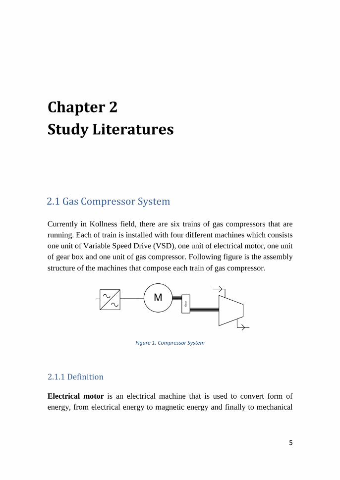
Currently in Kollness field, there are six trains of gas compressors that are

running. Each of train is installed with four different machines which consists

one unit of Variable Speed Drive (VSD), one unit of electrical motor, one unit

of gear box and one unit of gas compressor. Following figure is the assembly

structure of the machines that compose each train of gas compressor.

Figure 1. Compressor System

2.1.1 Definition

Electrical motor is an electrical machine that is used to convert form of

energy, from electrical energy to magnetic energy and finally to mechanical

6

energy [2]. Generally, electrical motor is formed by several parts such as rotor,

stator, shaft, end bells, bearing and motor housing as showed in Figure 2.

Figure 2. Electrical Motor Structure

Gear Gearbox is mechanical drives with step by step ratio change [2].

Mechanical drive is a unit set of mechanical power transmission that transfers

power from prime mover to the actuator. Gearbox contains several gears.

Gears are transmission mode with meshing or machines with toothed design.

Gears have function to transmit or receive motion from another gear-tooth.

When the gears are meshing with each other, they transmit torque moment, a

force that has tendency to rotate around the axis [3].

Figure 3. Example of Gearbox Design

7

Gas compressor is a method and devices for compressing gas. The gas is

compressed by entering an inlet which is known as Inlet Guide Vanes (IGV)

and accelerated by a row rotating airfoils (blades) called rotors and the

diffused, to obtain a pressure increase, in a row stationary blades called

stator[3]. A combination of a rotor and a stator makes up one stage and there

are several stages in a compressor. Figure 4 is showing the operating principle

for the compressor.

Figure 4. Compressor Components and Operating Principle

2.1.2 Failure Mode

Degradation from each machine will give impact to system’s performance. In

the next section, we will present the summary of several degradation processes

that can increase the failure rate for each component of gas compressor trains.

In table 1 we can see the list of failures that can deteriorate performance of gas

compressor system.

8

Table 1. Degradation Modes for Electrical Motor, Gearbox, and Gas Compressor

Unit Machine Category Faults

Electrical

Motor

Electrical Faults Open or short circuit in

winding

Wrong connection of windings

High resistance contact to

conductor

Unstable ground

Partial discharge

Mechanical Faults Broken rotor bars

Broken magnet

Cracked end-rings

Bent shaft

Bolt loosening

Bearing failure

Gearbox failure

Air-gap irregularity

Outer System Failure Inverter system failure

Unstable current source

Shorted/ Opened supply line

Gear Box Mechanical Faults Gear breakage

Flank damage

Gas

Compressor

Mechanical Faults Fretting

Creep deformation

Hot corrosion

Electrical Motor has three different types of degradation which are electrical

faults, mechanical faults and Outer system failure. Several faults that are

9

common to happen in electrical motor are partial discharge, bearing failure,

and broken rotor bars. Partial discharge (PD) is small electric sparks inside air

bubbles that are formed due to non-uniform electrical distribution on

insulation material [13]. This phenomenon usually happens in stator part of

electrical motor. In excessive electrical stresses, PD can cause change in

material properties to electrochemical reaction [14]. This changing causes

material degradation that eventually will lead to the complete breakdown of

the insulation [15]. Bearing of electrical motor can fail due to several causes

such as misalignment and fatigue that can lead to excessive vibration and

breakage, abrasion on the bearing due to improper lubrication, corrosion, and

contamination.

Gear breakage and flank damage are the main reason for a gear-box to have

decreasing performance. Gear breakage that represent statistically 60% of all

gear damages can be caused due to fatigue in tooth root, unit overload, and

inaccurate mounting that will lead to fracture of the gear. Another 40% of the

cause is flank damage. Flanks damage can happen due to pitting or surface

fatigue, loss of material, and high load that lead to plastic deformation.

Performance of gas compressor is mainly depending on performance of its

turbine blades. The fractures that happen on turbine blades will be unfavorable

for a gas compressor to maintain its performance. Fractures that happen on

turbine blades can be caused by several reasons such as fretting, creep

deformation and hot corrosion. Fretting is a wearing process between two

surfaces that has oscillatory motion with small amplitude [4]. Creep

deformation usually happens under operation condition where it is exposed to

high temperature yet still below the melting point of material. It also is

exposed with high stress level below the yield strength in long period of time

[9]. Turbine blades that are experiencing long high temperature and high stress

will stretch to the state that they will not be flexible anymore (plastic) or

become permanently deformed. Hot corrosion is an accelerated corrosion

process, causes by the existence of salt contaminants such as Natrium Sulfate

(Na2SO4), Natrium Chloride (NaCl), and Vanadium Oxide (V2O5). These

contaminants then are combined and create melted deposits and damage the

protective surface [10].

10

2.2 Remaining Useful Lifetime

The interests in this report are to predict the future failure before it actually

happens and estimate how much longer the machines can give the service

before they reach the end of their functional lifetime. The result from

prediction process or prognostic process can help the engineers to improve

their maintenance policy. It can give a valuable information for engineers to

decide and make plans for their maintenance strategies with better prediction

of future failure, better preparation on spare part components, and better

understanding of residual lifetime of the machines.

According to ISO 13381-1, prognostic is defined as “an estimation of time and

risk for one or more existing and future failure modes. The capability to

provide early detection of the precursor and/or incipient fault condition of a

component, and to have the technology and means to manage and predict the

progression of this fault condition to component failure.” [5] said that “failure

prognosis involves forecasting of system degradation based on observed

system condition”.

RUL as the result from prognostic process is defined as the length from the

current time to the end of the useful life [6]. In general, RUL also can be

formulated as follow [7] :

𝑅𝑈𝐿(𝑡) = 𝑖𝑛𝑓{ℎ: 𝑌(𝑡 + ℎ) ∈ 𝑆𝐿 | 𝑌(𝑡), 𝑌(𝑡) ∉ 𝑆𝐿 } (1)

Where 𝑌(𝑡) is system condition at time t and 𝑆𝐿 is set of failed states of the

unit.

The method of prognostic technique in this report is model-based. Model-

based prognostic methods mainly use the available mathematical or physical

models to picture the progress of the system from the working state to its

failure state. Model-based methods have the advantage to integrate physical

understanding of the system to improve the knowledge for system

degradation. The example of models that are using this approach are Markov

and Semi Markov model, Hidden Markov, Bayesian Network, etc.

11

2.3 Markov Process

2.3.1 Introduction

To solve the existing problems, it will be better if we can translate them into

models that can give description and represent the actual problems properly.

By having models, it will be easier to understand the main focus where we can

make limitations of contribution factors that will be included or not. The

limitations that we set will make the models simpler and allow us to do

experiments with possibility to change their parameters in order to seek the

optimum solution.

Markov chain is one of stochastic process {𝑋 (𝑡), 𝑡 ≥ 0} to model a system by

using states and transition between states [8]. Markov chain has Markov

property which means that the future event depends on the current state, not

its pass history. Variable 𝑋 (𝑡) is a random variable that denotes the state of

system at time 𝑡. Markov chain, based on time, is divided into discrete time

Markov chain and continuous time Markov chain. When time is discrete, it

may take value in {0,1,2,3, . . } or when we denote it by {𝑋𝑛, 𝑛 =

0, 1, 2, . . }. When time is continuous, we call it as continuous time Markov

chain or Markov Process. Markov process can be categorized as homogenous

and non-homogenous process. A model is called homogenous Markov process

when transition from one state to another state does not depend on time.

Otherwise, it will be called as non-homogenous Markov process.

We can start creating Markov process by defining several possible states and

transition rates between states. The simplest state is a state with status as

functioning state and not functioning or failed state. The transition from state

𝑖 to state 𝑗 can be denoted with 𝐴(𝑖, 𝑗). All of the transition rates in one process

then will be organized into a matrix 𝐴.

To know the probability in which state we are at time 𝑡 is always an interest

in Markov process. This is called transient probability that will be denoted

with 𝜇0 for initial state at time 0 and 𝜇𝑡(𝑖) denotes the probability that the

12

system is at state 𝑖 at time 𝑡. To calculate the value of 𝜇𝑡, we can use the

following formula

𝜇𝑡 = 𝜇0 𝑒𝑡𝐴 (2)

2.3.2 Multiphase Markov Process

The models of gas compressor trains will have different characteristics during

summer and winter period. In different periods, the system will have different

parameters of failure rates and these parameters will continuously change from

time to time between summer and winter. In order to depict the models close

to reality, we will use multiphase Markov process.

One summer in the initial year will be denoted by 𝑇1 which will represent time

𝑡 = 0 until 𝑡 = 4380. Winter time is from 𝑡 = 4381 until 𝑡 = 8760 and will be

denoted as 𝑇2. Next summer in second year will be denoted as 𝑇3, and so on.

In other word 𝑇𝑖 is time at which system will have season change. Since the

parameters of transition rates in summer and winter is different, transition

matrix 𝐴 for each phase will be different as well and will change at time 𝑇𝑖 .

To calculate the probability for such process, we can use this following

formula.

𝜇𝑡 = 𝜇0 𝑒𝑡𝐴1 for 𝑡 ∈ [0, 𝑇𝑖] and 𝑇𝑖 = 4380 (3)

Formula above is to calculate probability in operation process at time 𝑡 where

𝑡 starts from 𝑡 = 0 until 𝑡 = 4380, use transition matrix 𝐴1 that contains

transition rates that fit for summer period only. To continue the calculation for

next period, which is winter, we need to change transition matrix 𝐴1 to

transition matrix 𝐴2. Time 𝑡 in winter starts from 𝑡 = 4381 until 𝑡 = 8760.

The probability will be calculated as follow

𝜇𝑡 = 𝜇𝑇1 𝑒(𝑡−𝑇1)𝐴2 = 𝜇0 . 𝑒𝑇1𝐴1 . 𝑒(𝑡−𝑇1)𝐴2

13

for 𝑡 ∈ [4381, 𝑇𝑖] and 𝑇1 = 4380; 𝑇𝑖 for first winter which

is 𝑇𝑖 = 8760 (4)

For probability law at time 𝑡 then we can use formula as follow

𝜇𝑡 = 𝜇0 (∏ 𝑒(𝑇𝑘−𝑇𝑘−1)𝐴𝑘

𝑘=𝑖

𝑘=1

) 𝑒(𝑡−𝑇𝑖)𝐴𝑖+1

(5)

𝑘 denotes the phases.

14

15

Chapter 3

Maintenance Models

3.1 Markov Process Model without Degradation

3.1.1 Model without Maintenance

First model starts with very simple scheme. As is mentioned in the assumption

chapter 1, only two trains of gas compressor are used for the simplicity of the

model. In the beginning, three stages are included to see how long the system

will last from time 𝑡 = 0 until 𝑡 = 𝑇, where 𝑇 is time when all of the trains

are failed. In calculation with MATLAB, we use time horizon for 15 years or

(131400 hours) for 𝑇 to see the trend of the graphic that is created by numerical

results. This duration is used so that the probability to have all the trains failed

is close to 1. The initial state or state one of this Markov process model is a

condition where all the machines are perfect, second state or state two is a

condition where one machine is fail and one machine is still working. There

will be different status for this state in different season. The third state or state

3 is a failure state where both of the machines fail. In this model, there is no

maintenance is involved. For the first model or so called Model-1, is pictured

by Figure 5.

In one year, the trains are treated differently depend on the season, summer

and winter. During winter period, the trains is required to work in full capacity

16

to fulfil the required demand. Any failure in any train will make the whole

system fail since it will not be enough to cover the demand. Meanwhile in

summer, demand decreases. Thus, the structure of the trains during summer

can be varied. First option, all of the trains can be running yet not in full

capacity. Second option, half of the trains are functioning to fulfil the order,

and the rest are off for standby position in case there is a train that is failed

during operation.

Figure 5. Model 1 – Markov Process Model of The System Without Any Maintenance Program

Due to different capacity requirements between summer and winter, second

state of Markov model in both season has different status. It will be

functioning state in summer phase because we can still have option to make

the system work by manipulating the number of trains that need to be occupied

or switching the failed train with standby train or changing the rate of trains’

capacity to fulfil the required demand. Meanwhile during winter, the second

state of Markov model will become a failure state since all of maximum

capacity trains need to be functioning to reach the target. If we look at Model-

1, we notice that there are different colors in second state between summer

phase and winter phase to mark the status differences. First state in both phase

is colored blue to indicate working state. Second state is blue for summer

phase and white for winter. White circle indicates failure state.

17

To distinguish different availability between summer and winter, we make the

model into multiphase Markov model. From figure 5, we can see that there are

two phases of Markov model which are almost similar. First phase is named

summer phase and the other is named winter phase.

In computation using MATLAB, we define different phases of Markov

process with different transition matrix. A1 represents the transition between

states in summer phase only and A2 represents the transition between states in

winter phase only. Transition matrix A1 and A2 have three rows and three

columns corresponding to number of states in each phase. When 𝑎𝑖𝑗 is the rate

when we are leaving state 𝑖 to go to state 𝑗, then transition matrix 𝐴 can be

defined as follow

𝐴 = [

𝑎11 𝑎12 𝑎13

𝑎21 𝑎22 𝑎23

𝑎31 𝑎32 𝑎33

] (6)

For diagonal elements, the value 𝑎𝑖𝑖 = − ∑ 𝑎𝑖𝑗𝑟𝑗=0𝑗≠𝑖

where r is the last state of

the model. Transition matrix for Model-1 then will be

𝐴 = [−2𝜆 2𝜆 0

0 −𝜆 𝜆0 0 0

]

Since there is a different in working status from winter and summer, the

availability of the system in both period is calculated differently. Availability

of the system for time 𝑡 in period summer is accumulation of probability that

the trains, for time 0 until time 𝑡, are in state 1 and state 2 or we can write as

follow

𝐴𝑣(𝑡)𝑠𝑢𝑚𝑚𝑒𝑟 = 𝜇𝑡(1,1) + 𝜇𝑡(1,2) (7)

𝐴𝑣(𝑡)𝑤𝑖𝑛𝑡𝑒𝑟 = 𝜇𝑡(1,1)

𝜇𝑡 is probability of Markov process in each state. Thus, for initial probability

of the system is 𝜇(0) = [1 0 0] which means all of the trains are in the

first state. In equation (8), 𝜇𝑡(1,1) referring probability in row 1 column 1.

18

From one state to another state, the transition rates that are used are following

data from OREDA as the table 2 below. OREDA that is referred in this report

is OREDA 6th Edition (2015) Volume 1 – Topside Equipment.

Table 2 – System Failure Rate from OREDA

Machine Total Failure rate

(Per 10-6 hours)

Degraded Failure rate

(Per 10-6 hours)

Variable Speed Drive 10 3.5

Electrical Motor 114.91 38.3

Gear Box 15 5.25

Gas Compressor 524.46 193.89

Total 664.37 240.94

Thus, total failure rate for the system is total accumulation from four failure

rates of composer machine units, which is 6.6437 x 10-4/hours. Notice that the

transition matrixes are the same for both phases, indicate that transition rates

from state one to state two and from state two to state three is the same.

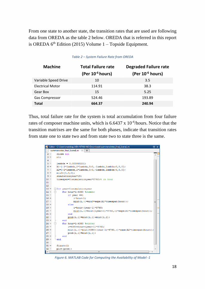
Figure 6. MATLAB Code for Computing the Availability of Model -1

19

Using MATLAB program, we can calculate the availability of the system

based on Markov process that we have built. In figure 6, we see MATLAB

code to compute system’s availability in each phase. Each phase or each

season is designed to take place for six months’ period or 4380 hours. The

availability diagram from numerical result of Model-1 is showed in Figure 7.

Figure 7. The Availability Graph for Model 1

From Table 2, we know that total failure rate is 𝜆 = 6,6437 ×10−4 /ℎ𝑜𝑢𝑟𝑠 ,

it means that the system has mean time to failure (MTTF) for 1505.18 hours.

As we expect, the system will have total failure before it reaches second year

of operation. To see the trend in longer period, the adjustment to failure rate

is made. By using ten (10) time smaller 𝜆 value from OREDA, we can see the

trend result in figure 8.

We start computing the model with summer phase first, then continue to winter

phase, and go back to summer phase for the next year. From the graph in figure

8, we can see the dropping line for winter season is quite extreme. The gap

between phases due to different condition for working state in each season. In

fifteen years, the availability line for Model 1 is closed to 0.

0

0.2

0.4

0.6

0.8

1

16

09

12

17

18

25

24

33

30

41

36

49

42

57

48

65

54

73

60

81

66

89

72

97

79

05

85

13

91

21

97

29

10

33

71

09

45

11

55

31

21

61

12

76

91

33

77

13

98

51

45

93

15

20

11

58

09

16

41

7

AV

AIL

AB

ILIT

Y A

T TI

ME

T

TIME (T) IN HOUR(S)

Availability Diagram for Model-1 (λ=6,6437 x 10-4)

Availability Line

MTTF = 1505.8 hours

20

Figure 8 The Availability Graph for Model 1 Using Adjusted Failure Rate

3.1.2 Markov Process Model with Maintenance

Model 2

Model-1 above is very basic and does not consider any maintenance.

Adjustment is needed to make the simulation can give a proper result to real

case. Model-2 in figure 9 is a model that is created with involvement of

maintenance when the system is failed. In this model, when the failure

happened during winter at state 2, maintenance will be carried out. Yet, when

the period of maintenance in this state start entering summer phase, the

maintenance will be hold on or stopped because in summer phase we need

fewer trains. In summer phase, we define second state as a working state where

one failure train will keep the system goes on so the maintenance will be no

longer needed.

Repair rate is simulated with two numbers of repair values i.e. maximum

repair time (0.0027/hour) and mean repair time (0.04/hour) from OREDA. The

result can be seen in Figure 10.

21

The graphs in Figure 10 are numerical result of Model-2 with different value

of repair rates, maximum and average repair time. The total mean availability

of each model in order is 75.426%, and 97.761%. The explanation about how

to calculate mean availability value will be discussed in chapter 3 section 3.3.1

availability comparison. Despite of the result from Model-2 with average

repair time is quite high, however in certain time when the system switches

the phase to winter, the availability is close to 0. This is not the risk that a

company will take because it can lead to failure for every winter phase. When

we adjust the value of failure rate become ten (10) times smaller than the value

from OREDA, we get result that is pictured on Figure 11.

In figure 10, we can see that the pattern of the graph gets steady in short period

of time. We start the graph in summer phase at 1 of y axis. It goes down really

slow for the first phase and suddenly drop with big gap when the system

switches to winter phase at 𝑡 = 4381. This happens since we calculate the

availability from first state only during winter phase instead of first state and

second state like we do in summer phase. The availability line in winter

increases rapidly until it gets stable number. The increase happens since value

of repair rate is bigger compare to failure rate. When the phase enters summer

period in the following year, the availability line jumps higher since we come

back to initial calculation, counting the availability from probability in the first

and second state. The pattern goes on until in the end of time horizon used in

this computation

Figure 9. Model 2 – Markov Process With Maintenance

22

Figure 10. Numerical Result for Model 2 with Different values of Repair Rate

.

Winter phase

Summer phase

Summer phase

Winter phase

23

Figure 11 Availability Diagram for Model 2 with Maximum Repair Rate and Adjustment of Failure Rate

Total availability of the system in Model-2 with adjustment failure rate and

maximum repair time is 95.751% and 99.696% for Model-2 with adjustment

failure rate and average repair time. We can see that in every model, we can

get steady state in short time, starting at year 2 or year 3. This fast formation

of steady state occurs due to few number of phases which are only summer

and winter and numerical result from the same phase is similar for every year.

Model 3

In Model 3, we introduce maintenance program as soon as any failure happens

to the running trains. In this case, we assume one maintenance crew is

dedicated to each failed train and repair rates are the same for both phases.

Model 3 is depicted on Figure 12.

24

Figure 12 Markov Process Model 3, Availability Diagram for Model 3 in Average (Middle) and

Maximum (Bottom) Repair time.

25

The availability for the system from Model-3 is quite high i.e. 80.265% with

maximum repair rate value and 98.365% with mean repair rate. The

availability diagram for each model is showed in Figure 13. The availability

during summer and winter is plotted with straight line because the repair rate

is higher than failure rate so the trains can maintain their constant condition

almost as initial state. The dropping line in availability line during winter

phase due to the number of state that is considered as working state which is

only the first state.

Model 4

we change maintenance strategy into full maintenance which means that we

repair the trains and turn them to new condition or we assume they turn as

good as new after maintenance. The maintenance will be done when the whole

system is failed. During summer, the system fails in the third state. Meanwhile

in the winter, we define system failure in the second state and third state. Since

in third state of winter phase all of the trains are failed, we need faster repair

rate, thus we arrange value of 𝜇1 is higher compare to 𝜇2. The availability

with this maintenance program is 84.234%.

Figure 13. Markov Process - Model 4

26

Figure 14. Model 4 and Availability Diagram for Model 4

Model 5

In this model, we conduct maintenance service as soon as any failure happens

and return the trains to their last position when the system is in working state.

With this program, we get better result compare to Model 4 result. The

availability with this model is 97.696%

27

Figure 15. Model 5 and the Availability Diagram

Model 6

In this model, we try to apply maintenance action as soon as any failure is

happened. Slightly different compare to Model 5, instead of we repair the

failed trains to the last position, in this model we return the trains as good a

new like in the first state. This program gives the better result compare to the

other model that has been described above. Using maximum repair time value,

we can get availability of the system for 82,391% and when the mean repair

time is used, the availability is 98,391%. The model and the numerical result

diagram can be seen in figure 16.

28

Figure 16. Model 6, Availability Diagram with Maximum Repair Time and Mean Repair Time

Model 7

The first six models above have the same scheme for winter phase. It has only

one working state i.e. the first state. During winter phase the system is able to

fulfil the order when all of the trains are in good condition and running in their

full capacity. But more often in real case, one failure of the train will not make

the rest of the trains stop operating. They will keep running. Speedy

maintenance action however will be required in this situation to put the system

29

back on track as soon as possible. While the failed train is under maintenance,

the company will endure some loss since they cannot meet the target.

Figure 17. Model 7 - Markov Process Model

Model-7 is calculated to see how the difference in availability for the whole

system when we make the second state of winter phase turn into working state.

In Figure 17, the repair rate for 𝜇1is smaller compare to 𝜇2. During winter

phase, all the trains are required to be in place to fulfil the order. Thus,

maintenance is more urgent and has to be done faster. In this case, the value

of 𝜇2 and 𝜇3 are using mean repair time from OREDA and 𝜇1is using

maximum repair time value

Figure 18 displays two different availability diagrams for winter phase only.

One diagram is showing the availability of the system when it is running with

full capacity with average availability 96.63%, and the other one is showing

the availability of the system when it is in the second state with system

capacity is reduced. The average availability is 3.3% for reduced capacity. In

total, the average availability of the system, including summer phase is

increase to 99.75%.

When both of phases have the same working state, the gap between summer

season and winter season is narrower and availability of the system is

increased. But we need to consider that there is also cost for production. From

this numerical result, we can estimate the approximation of production lost

30

probability that company will face during winter operation. To get this

estimation number, we calculate total availability of the system during winter

phase when the system in state two and divided the number to total availability

of the system. From this division, we get 1.6% from total availability as

estimation number for production lost. Knowing this estimated production

lost, the company can make planning earlier to cover the lost, for instance is

by having buffer for the gas that need to be delivered to the customer.

Figure 18. Availability Diagram for Model 7 (Winter Phase). Availability Diagram for state 1 (top) and state 2 (bottom)

31

3.1.3 Simulation with Standby Condition

Model 8

As was mentioned before, the treatment for the gas compressor trains during

summer may vary. Another maintenance program that is adopted in this case

is standby trains model. Standby model allows us to cut maintenance time by

having trains exchange. The train that is failed will be replaced by good train

as soon as the failure happens. With this planning, the repair time during

summer can be smaller compare to winter time. In the model, we set 𝜇1 > 𝜇2 .

The mean availability for Model-8 is 85.348%.

Figure 19. Model 8 - Markov Process Model and Availability Diagram

32

3.2 Markov Process Model with Degradation Process

Model 9

First section of this chapter presents system models without any degradation

process. There is no observation or monitoring applied to the system before

the system actually fails or breaks down. Monitoring activity towards

degradation process in each machine can give advance warning to engineers

that there will be digression in system performance. The engineers will be able

to take preventive actions to avoid the unwanted event, system failure.

Figure 20. Model 9 – Markov Process Model with Degradation State

The models that are discussed in this section will give illustration on how the

actions that are taken place to respond any degradation process will influence

the availability number. Figure 20 shows the expansion of Markov process by

having degradation states before the trains move to failure state. Performance

of the machines will decrease rapidly after the machines experiencing

degradation. Thus, the failure rate for 𝜆2 is higher compare to 𝜆1. By having

33

the knowledge of trains’ current state, we can have better planning for the

maintenance such as advance planning for spare part supply, integrated

maintenance schedule, proper number of required maintenance crew, and

better coordination with another operation schedule.

In model 9, maintenance or repair activity is implemented as soon as the

failure happens. Both phases have the same program maintenance. Yet, there

is different rate for 𝜇1 and 𝜇2 since maintenance action during winter is more

urgent and needs to be done faster.

Figure 21. Avaialbility Diagram for Model 9

As expected, the mean availability for model 9 is quite high i.e. 98.30%. We

calculate the availability from 5 states out of 6 states for summer phase where

total failure will happen when both of the machines are failed in the same time.

During winter, only 3 states out 6 states for winter phases that are considered

as working states where all of the trains need to be in function.

34

System failure will less likely to happen in this model since monitoring actions

of the machines are more frequent and the operators will have more attention

to the machines once degradation symptoms start emerging.

Model 10

In the last model of this report, we will introduce preventive maintenance.

Preventive maintenance will be done when the maintenance crews have

identified that there is degradation happening in the trains. In Figure 22 we

can recognize preventive maintenance for green arrow from state from state

CdC or CdCd to initial state, CC. Since preventive maintenance is an early

detection process to avoid further failure, maintenance action not necessarily

to be done so fast. Thus, in this model, we set repair rate of preventive

maintenance with same value of maximum maintenance time from OREDA

(𝜇 = 0,0027/ℎ𝑜𝑢𝑟). Numerical result for this calculation, it gives average

availability for 99.568%. It approves that by having preventive maintenance,

we can keep our system always in working condition most of the time.

35

Figure 22. Model 10 - Markov Process Model with Preventive Maintenance

36

3.3 Model Recommendation from Availability

Comparison

We have ten models that have been presented in this chapter to give the

company information regarding availability for maintenance programs that

can be implemented in the plant. Those models are considered possible to be

applied in real technical condition on the existing gas compressor system even

though the parameters value that are used need to be adjusted with the real

number from the plant. Currently, there are no actual data that can be referred

to, thus some of the parameters in this report are based on assumption and

some of data are also referred to OREDA data base. To avoid unreasonable

gap in comparing the availability between models, we will compare one model

to another model that uses the same parameters assumption.

Table 3

Maintenance Program

Mean Availability

per unit time

No Repair Time Model 1-1 1.60 %

Model 1-2 11.49 %

Maximum Repair Time (μ=0,0027/hour)

Model 2-1 75.43 %

Model 3-1 80.27 %

Model 6-1 82.96 %

Mean Repair Time (μ=0,04/hour)

Model 2-2 95.75 %

Model 3-2 98.37 %

Model 6-2 98.39 %

Combination of Repair Time Model 4 84.23 %

Model 5 83.73 %

Reduced-Capacity Model 7 99.75%

Standby Model 8 85.35%.

Degradation Model 9 98.30%

Model 10 99.57%

37

These average availability numbers are produced by following this formula:

𝐴𝑣𝑒𝑟𝑎𝑔𝑒 𝐴𝑣𝑎𝑖𝑙𝑎𝑏𝑖𝑙𝑖𝑡𝑦 =∑ 𝜇𝑡

𝑡=131400𝑡=0

131400 ℎ𝑜𝑢𝑟𝑠 (8)

From MATLAB calculation, we will get 3 columns information of 𝜇𝑡. Each

column contains information for each state. Only 𝜇𝑡 in working state will be

considered. During summer, information from state one and two will be added

up together. Meanwhile for winter, 𝜇𝑡 for first state only that will be put into

account. Total availability during winter will be summed with total availability

of summer. Total number from this addition then will be divided by total time.

Model 2 and 3 share the same parameters assumption for failure rates and

repair rates, both in summer and winter phase. Repairs in both models are done

when failures happen and turn the trains back to previous condition. Model 6

is also almost similar with model 2 and 3 except we assume that reparation of

the trains will turn the trains’ condition as good as new. The models are

calculated for two repair time, maximum repair time and average repair time

that we get form OREDA.

All of the models except model 7 have the same assumption for working state

in winter phase. Gas compressor trains in winter season must not fail to fulfil

the order. Thus, if one train fails then the system is considered fail as well.

This assumption makes the availability in winter season only calculated from

state one. Model-7 gives the highest average availability value, yet we have to

consider the lost production that occurs.

For standby model, Model8, is similar with the condition that we have in

Model-5. The difference is in summer. Instead of let all the machines are

functioning, model in standby mode allows half of the trains to be in standby

position so if any train fails during the operation, the operators can switch the

train with standby train and repair the failed train in parallel. This model gives

slightly higher availability in total. It also helps operators to more focus in

repairing since they will have more time until the next failure.

38

Preventive model that is explained in Model 10 is showing the best availability

number. It has been expected for having machine degradation monitoring. it

will give better information for the operators to avoid the system failure. With

this information, we can have better plan in maintenance and other strategies

related to maintenance to make the operation optimum.

39

3.4 Model Validation

To be sure that models in this chapter are correct, we need to validate the

models. One of the way to validate the models is by comparing the numerical

results with results from another tool or software. Here, we will use another

software called GRIF to check the numerical results from models that are

processed by MATLAB. GRIF is one of many software that can be used to

calculate Markov process. By inputting the Markov process graphs, we able

to calculate the availability of the system. For an example, we will use model

8 to see whether the numerical results that we get from MATLAB and GRIF

are the same or not. In previous section, it has been mentioned that average

availability for Model 8 is 85.348%

Figure 23. Diagram Comparison between GRIF (top) and MATLAB (bottom)

40

Figure 23 is showing graphs comparison that is produced by GRIF and

MATLAB software. We can see that both programs give similar result. In

GRIF’s diagram, we can see the information related to average value of the

availability which is 0.8534 or 85.34%.

We also compare the numerical result between GRIF and MATLAB per time

(t) in figure 24. Error between two software in average is 0.073%. This number

is small enough and acceptable to say that the result from both software is the

same. In other word, the models that we create with MATLAB are valid.

Comparison for other models will be presented in Attachment Chapter except

for Model 9 and Model 10 due to graphics limitation in GRIF. Graphics

limitation in GRIF means how much number of states and transition rates that

we can calculate. GRIF has limitation for 25 graphics and Model 9 and Model

10 have more than the limitation allowed.

The spikes that are showed in figure 24 happen in the time when the phases

are switching from summer to winter or winter to summer (𝑇𝑖). To calculate

the error, we use this following formula

% 𝐸𝑟𝑟𝑜𝑟 = |µ𝑡 𝐺𝑅𝐼𝐹−µ𝑡 𝑀𝐴𝑇𝐿𝐴𝐵

µ𝑡 𝐺𝑅𝐼𝐹| ×100 (8)

Figure 24 - Error Diagram Between GRIF and MATLAB

41

In summary, the comparisons between numerical results that are produced by

GRIF and MATLAB are showed in table 4.

Table 4. Comparison of Availability Between GRIF and MATLAB

Model % Error

Mean Availability per Time (t) in % Description

GRIF MATLAB

1 72.71823 1.6 1.6

2 4.480605 78.24 75.43 µ=0,0027/hour

2 0.036443 97.79 95.75 µ=0,04/hour

3 0.000787 80.27 80.27 µ=0,0027/hour

3 2.03E-07 98.37 98.37 µ=0,04/hour

4 9.03E-06 84.23 84.23

5 1.627436 85.29 83.73

6 2.61E-05 82.96 82.96 µ=0,0027/hour

6 2E-07 98.39 98.39 µ=0,04/hour

7 0.014278 98.1 99.75

8 0.073007 85.34 85.35

To calculate the availability using GRIF is much simpler compare to

MATLAB. GRIF has input interface that allows the user to create Markov

process graph directly in the program.

Figure 25.GRIF’s User Interface

Computation Button

42

The brown circles identify the states that are available and white circles

identify the failure states. The user can connect one state and another using the

arrows for transition direction. It is possible to rename the state and change

the efficiency of the state. For normal state, without degradation, usually the

efficiency is 1.

To adjust the parameter, GRIF also has several columns that we can fill to set

the duration of the simulation, single Markov Process or multiple process, etc.

Using computation button, the program will start computing the availability

of the process that has been input. The result can be a graph or set of number

that shows the availability of the system in each 𝑡 according to time setting.

43

Chapter 4

Conclusion

In this chapter, we will look back the objectives of this thesis and will discuss

whether we have answered all the points which are mentioned in that section.

In Objectives, we have five main points which are list of possible programs,

availability estimation, availability comparison, remaining useful lifetime

estimation, and maintenance program that will be recommended for the

company.

4.1 Maintenance Models

We have discussed ten (10) models of Markov process with different number

of parameters and different scenarios. MATLAB is used to help as calculator

in producing numerical results for computing the probability of the system in

each state at time 𝑡. The time period that is calculated is for fifteen (15) years.

Adjustment in each model is applied to make the model applicable for real

condition. Since we do not proper information related to failure rates and

maintenance time for real case, we use data from OREDA. There are several

models that are calculated twice with different parameters to see how big the

influence of a parameter to change system’s availability.

44

4.2 System Availability

We define the model using Markov process by divided the physical conditions

(working or fail) of the system into several possible states. Between each state,

we set different parameters and assumptions such as value of transition rate,

when maintenance action will be done, and the result of maintenance action

toward the failure trains (as good as new or not). Different phases are applied

to distinguish different conditions of states due to difference in demand

requirement.

Using MATLAB as calculator, we can get numerical result on possibility of

the system is exist in certain state, in this case we interest to know the

possibility of the system exist in working state regardless in which phase.

Different models share different trends on the graph. The highest availability

is showed by model 10 where there is involvement of preventive maintenance

and condition monitoring towards machine’s performance.

Condition monitoring let us to have better knowledge of the system that we

have. It gives us earlier warning when the system start degrading so the crew

can take action as soon as possible before further unwanted event occurs. With

early information about what happen to gas compressors, the operators can

decide what actions that need to be done in proper and timely manner.

The results that are produced from MATLAB are validated using GRIF.

Another software that has capability in computing availability from Markov

process. In chapter 3.4, we can see the that our calculation using MATLAB

gives the same result if we use this software.

4.3 Remaining Useful Lifetime

Remaining useful lifetime is the remaining time that a system has until the end

of useful life knowing the condition at current time. To estimate remaining

useful lifetime with Markov process, we have to know the current state of the

system.

45

Initial probability for every state at time t=0 is µ0 = [1,0,0]. When we compute

Markov process model, we assume that the system starts with new machines

so we can be sure that the system is 100% work. In real condition, the system

may have run for several years, so we have to adjust the value of µ0 and

compute the model again. With the same procedure in the chapter 3.1.2, we

can see the probability of the machine is being in working state for period of

time that become our main interest.

Let’s take Model-2 for example. When the system has run for 20 years, and

we assume that in current condition, the probability of each state for the system

is µ0 = [0.3,0.65,0.05]. Our interest is to know the availability of the system

in the next 5 years. Using MATLAB, we can get estimation for 0.1539 or

15.4% that the system will be available for the next five years.

Figure 26. Availability Estimation for a System

46

4.4 Further Discussion

While writing this thesis, there are some points that become interest for the

writer yet not have been covered or discussed. This interest can be input for

the reader to explore more related to those topics. First, numerical results from

all of the models show that they reach steady state in early time. It may be

due to repair rate that is quite high, few number of phases which are only two,

and also because the assumptions that are used for repaired condition. In this

report, it is assumed that after repair or maintenance, the trains come back to

new condition which may not be the case in real condition.

Second, condition monitoring is a good tool in supporting Model-10 as the

recommended model that the writer proposed for this report. There are a lot of

technics of condition monitoring that will be fit to be carried out for gas

compressor system. This topic can be an option for another study in the future.

There are no data yet from the actual plant that can be useful for this report.

Necessary adjustment need to be done when the required information will be

available.

47

Attachment

In this section, we will present the comparison of Error computation from

GRIF and MATLAB that have been explained in chapter 3.4.

Model 1

In the beginning of the graph, the errors are close to 0. After 2 years, the errors

increase. This is because numerical results from MATLAB for µ𝑡 keep

decreasing into so small number (µ131400 = 1.555 𝐸 − 76). Meanwhile with

computation using GRIF, the values of µ𝑡 decrease only at 𝑇𝑖 or when the

season switches yet within each season the values remain constant. For

example, the values from µ127021 until µ131400 are the same i.e. 6.5836 E-14.

This different that make the error after two years decrease. The average of %

error for Model 1 is 72,72%. Availability diagram for Model 1 by GRIF is

presented in the next page.

0

20

40

60

80

100

14

86

89

73

51

46

02

19

46

92

43

36

29

20

33

40

70

38

93

74

38

04

48

67

15

35

38

58

40

56

32

72

68

13

97

30

06

77

87

38

27

40

87

60

79

24

74

97

34

11

02

20

81

07

07

51

11

94

21

16

80

91

21

67

61

26

54

3

Erro

r P

er T

me

(t)

in %

Time in Hour(s)

% Error Between GRIF and MATLAB(Model 1)

48

Model 2

The average of error for Model 2 is 0,036% for Model 2 that use repair rate

equal to 0,04/hour. And for Model 2 that uses maximum repair rate, the

average of error is 4,48%. There is quite different results between GRIF and

MATLAB even though the trend from availability diagram for both method

are similar.

0

5

10

15

20

25

1

48

68

97

35

14

60

21

94

69

24

33

6

29

20

33

40

70

38

93

74

38

04

48

67

1

53

53

85

84

05

63

27

26

81

39

73

00

6

77

87

38

27

40

87

60

79

24

74

97

34

1

10

22

08

10

70

75

11

19

42

11

68

09

12

16

76

12

65

43

Erro

r P

er T

ime

(t)

in %

Time in Hour(s)

% Error Between GRIF and MATLAB(Model 2 µ=0,0027/hour)

49

The spikes in both two diagrams above happen during phase changing.

0

0.5

1

1.5

2

1

54

76

10

95

1

16

42

6

21

90

1

27

37

6

32

85

1

38

32

6

43

80

1

49

27

6

54

75

1

60

22

6

65

70

1

71

17

6

76

65

1

82

12

6

87

60

1

93

07

6

98

55

1

10

40

26

10

95

01

11

49

76

12

04

51

12

59

26

Erro

r P

er T

ime

(t)

in %

Time in Hour(s)

% Error Between GRIF and MATLAB (Model 2 µ=0.04/hour)

50

Model 3

The trend for Model 3 between maximum repair time and average repair time

shows the same pattern. The average error for Model 3 in consecutive order is

0.000787036 % and 2.03181E-07%. Different results between GRIF and

MATLAB occur in the beginning of computation. While the model gives

steady state result, the errors are close to 0.

0

0.001

0.002

0.003

0.004

0.005

0.006

0.007

15

05

5

10

10

91

51

63

20

21

72

52

71

30

32

53

53

79

40

43

34

54

87

50

54

15

55

95

60

64

96

57

03

70

75

77

58

11

80

86

58

59

19

90

97

39

60

27

10

10

81

10

61

35

11

11

89

11

62

43

12

12

97

12

63

51

Erro

r P

er T

ime

(t)

in %

Time in Hour(s)

% Error Between GRIF and MATLABModel 3 (µ=0,0027/hour)

0

0.0001

0.0002

0.0003

0.0004

0.0005

0.0006

15

05

51

01

09

15

16

32

02

17

25

27

13

03

25

35

37

94

04

33

45

48

75

05

41

55

59

56

06

49

65

70

37

07

57

75

81

18

08

65

85

91

99

09

73

96

02

71

01

08

11

06

13

51

11

18

91

16

24

31

21

29

71

26

35

1

Erro

r iP

er T

ime

(t)

in %

Time in Hour (s)

% Error Between GRIF and MATLABModel 3 (µ=0,04/hour)

51

Model 3 with µ = 0,0027/hour

Model 3 with µ = 0,04/hour

52

Model 4

The average of error is 9.02595E-06%.

0

0.0005

0.001

0.0015

0.002

15

25

71

05

13

15

76

92

10

25

26

28

1

31

53

73

67

93

42

04

94

73

05

52

56

1

57

81

76

30

73

68

32

97

35

85

78

84

1

84

09

78

93

53

94

60

99

98

65

10

51

21

11

03

77

11

56

33

12

08

89

12

61

45

Erro

r P

er T

ime

(t)

in %

Time in Hour(s)

% Error Between GRIF and MATLABModel 4

53

Model 5

The average of error is 1.627435649%.

00.5

11.5

22.5

33.5

4

1

50

55

10

10

9

15

16

3

20

21

7

25

27

1

30

32

5

35

37

9

40

43

3

45

48

7

50

54

1

55

59

5

60

64

9

65

70

3

70

75

7

75

81

1

80

86

5

85

91

9

90

97

3

96

02

7

10

10

81

10

61

35

11

11

89

11

62

43

12

12

97

12

63

51

Erro

r P

er T

ime

(t)

in %

Time in Hour(s)

% Error Between GRIF and MATLAB(Model 5)

54

Model 6

The average of error is 1.99989E-07% for µ = 0,0027/hour and 2.60589E-

05% for µ = 0,04/hour

0

0.001

0.002

0.003

0.004

0.005

0.006

0.007

15

05

5

10

10

91

51

63

20

21

72

52

71

30

32

53

53

79

40

43

34

54

87

50

54

15

55

95

60

64

96

57

03

70

75

77

58

11

80

86

58

59

19

90

97

39

60

27

10

10

81

10

61

35

11

11

89

11

62

43

12

12

97

12

63

51

Erro

r P

er T

ime

(t)

in %

Time in Hour(s)

% Error Between GRIF and MATLABModel 6 (µ=0,0027/hour)

0

0.0001

0.0002

0.0003

0.0004

0.0005

0.0006

15

05

51

01

09

15

16

32

02

17

25

27

13

03

25

35

37

94

04

33

45

48

75

05

41

55

59

56

06

49

65

70

37

07

57

75

81

18

08

65

85

91

99

09

73

96

02

71

01

08

11

06

13

51

11

18

91

16

24

31

21

29

71

26

35

1

Erro

r P

er T

ime

(t)

in %

Time in Hour(s)

% Error Between GRIF and MATLABModel 6 (µ=0,04/hour)

55

Model 6 with µ = 0,0027/hour

Model 6 with µ = 0,04/hour

56

Model 7

The average of error is 0.014277547%.

0

5

10

15

20

25

30

1

48

68

97

35

14

60

21

94

69

24

33

6

29

20

33

40

70

38

93

74

38

04

48

67

1

53

53

85

84

05

63

27

26

81

39

73

00

6

77

87

38

27

40

87

60

79

24

74

97

34

1

10

22

08

10

70

75

11

19

42

11

68

09

12

16

76

12

65

43

Erro

r P

er T

ime

(t)

in %

Time in Hour(s)

% Error Between GRIF and MATLABModel 7

57

Bibliography 1. StatOil, StatOil. 2013. 2. Randall, R.B., A New Method of Modeling Gear Faults. Journal of Mechanical

Design, 1982. 104(2): p. 259-267. 3. Jelaska, D., Introduction, in Gears and Gear Drives. 2012, John Wiley & Sons,

Ltd. p. 1-16. 4. Kermanpur, A., et al., Failure analysis of Ti6Al4V gas turbine compressor

blades. Engineering Failure Analysis, 2008. 15(8): p. 1052-1064. 5. Jianhui, L., et al. Model-based prognostic techniques [maintenance

applications]. in Proceedings AUTOTESTCON 2003. IEEE Systems Readiness Technology Conference. 2003.

6. Kassner, M.E. and M.T. Pérez-Prado, Five-power-law creep in single phase metals and alloys. Progress in Materials Science, 2000. 45(1): p. 1-102.

7. Barros, A.C.P., Some notes about the Remaining Useful Lifetime. 2016: NTNU. p. 2.

8. Rausand, M. and H. Arnljot, System reliability theory: models, statistical methods, and applications. Vol. 396. 2004: John Wiley & Sons.