1

Remarks on the exact energy functional for fermions: an

analysis using the Löwdin partitioning technique

Marc Caballero,a,b Ibério de P. R. Moreira,a,b Josep Maria Bofilla,c,*

aInstitut de Química Teòrica i Computacional, Universitat de Barcelona, IQTCUB,

C/ Martí i Franquès 1, E-08028 Barcelona, Spain bDepartament de Química Física, Universitat de Barcelona,

C/ Martí i Franquès 1, E-08028 Barcelona, Spain cDepartament de Química Orgànica, Universitat de Barcelona,

C/ Martí i Franquès 1, E-08028 Barcelona, Spain *Corresponding author. Email: jmbofill@ub.edu

(Version: August 29, 2013)

Abstract.-

A comparison model based in the Löwdin partitioning technique is used to

analyze the differences between the wave function and density functional models. This

comparison model provides a tool to understand the structure of both theories and its

discrepancies in terms of the subjacent mathematical structure and the variationality

required for the energy functional. It is argued that the density functional theory can be

compared to the wave-function theory. The wave-function theory provides an explicit

form of the exact energy functional for a fermion system from the Full Configuration

Interaction approach. The density functional theory can be seen as special cases of

Löwdin function that do not satisfy all variational conditions on and also on the

term. This analysis shows that ignoring the restrictions imposed by the spin and

space symmetry requirements of the solutions when making a variational calculation

implies that the correlations expressed by the function will be inconsistent with a

function derivable from a spin and space symmetry adapted wave function

, even for a closed-shell system. The comparison scheme also provides a

new insight in order to achieve a consistent description of the molecular electronic

structure of both ground and excited states. Some numerical results are reported.

Keywords: wave-function theory, density functional theory, Löwdin partition

technique, variational methods, comparison model.

ρ(r)

EXC

ρ[ ]

ρ(r)

γ1(r1;r1')

Ψ(r1s1,,r

nsn)

2

1. Introduction.

The quantum many-electron system defined by n electrons and N nuclei in

interaction is one of the central problems in chemistry and physics. The fundamental

mathematical formulation of the non-relativistic n electron problem is the time

independent Schrödinger equation for this system and the corresponding exact solutions

provide the essential quantum-mechanical description of each electronic state in terms

of the different n electron wave function Ψ(r1s1,,r

nsn) .

For a system of n electrons and N nuclei in interaction, the time independent

Schrödinger equation (in the Born-Oppenheimer approximation) can be written as a

Rayleigh-Ritz quotient given by

E Ψ[ ] =Ψ H Ψ

Ψ Ψ (1)

in which the Hamiltonian operator is defined as

H = T + V + W (2)

with

In this expression, the first term stands for the electrons kinetic energy of the electrons,

the second arises from the external potential v(ri;R1; ··· ;RN) generated by the nuclei and

1/rij is the two electron interaction. This hamiltonian operator defines, along with its

boundary conditions, an eliptic second order differential equation and the wave-function

must satisfy some specific conditions to be an acceptable solution of Eq. (1), namely: a)

must be bounded and continuous, b) the partial derivatives with respect

to spatial coordinates must be continuous, and c) the function

| |2 must be integrable. Since the non-relativistic many-electron

Hamiltonian does not act on spin coordinates, anti-symmetry and spin restrictions must

be imposed ad hoc to restrict the solutions (i.e. the wave functions Ψ(r1s1,,r

nsn) ) to

T (r1,,r

n) = −

1

2∇(i )

2

i=1

n

∑

V (r1,,r

n;R

1;;R

N) =

−ZI

RI− r

iI =1

N

∑i=1

n

∑ = v(ri;R

1;;R

N)

i=1

n

∑

W (r1,,r

n) =

1

ri− r

jj= i+1

n

∑i=1

n−1

∑ =1

riji> j=1

n

∑

Ψ(r1s1,,r

nsn)

Ψ(r1s1,,r

nsn)

3

the set of functions that satisfy the Pauli principle and spin symmetry requirements of

the quantum mechanical state of the system.

In the wave-function theory (WFT) formalism, the most compact expression for

the energy of the n-electron system in the field of N fixed nuclei can be written as

(3)

in which the many electron quantities γ1(r1) and γ2(r1,r2) are the diagonal elements,

γ1(r1) = γ1(r1;r1) and γ2(r1,r2) = γ2(r1,r2;r1,r2), of the spinless one- and two-electron

density matrices, respectively [1-3] The function γ1(r1) = γ1(r1;r1) corresponds to an

observable, the one electron density ρ(r), and is commonly used in electronic structure

theory. In WFT, large efforts are devoted to obtain accurate prediction of the energy of

a given system in a given electronic state using a reasonable estimate of Ψ(r1s1,,r

nsn) .

It is customary to expand Ψ(r1s1,,r

nsn) in a known basis set and to find the expansion

coefficients using the variational method and with all necessary and sufficient

constraints (spin and space symmetries) to prevent the variational collapse [4]. This

mathematical requirement is essential to avoid to converge to a solution with no

physical meaning. This is the basis of the so-called Full Configuration Interaction

(FCI) method which provides the exact solution for the energy functional of the

electronic system defined in Eq. (3) in a given basis set. Indeed, for a finite basis set

this is the exact solution and has been extensively used as a benchmark for quantum

chemical methods [5,,,,9].

Density Functional Theory (DFT) propose a different approach which aims to

replace both γ1(r1;r1’) and γ2(r1,r2) in Eq. (3) by the one-electron density, γ1(r1). For the

ground state, this wish is justified by the celebrated Hohenberg-Kohn theorems (HK),

which state that the exact ground state total energy of any many-electron system is

given by a universal, unknown, functional of the electron density only [10]. Rigorously

speaking, only the second term of the right hand side part of Eq. (3) is an explicit

functional of the diagonal one-electron density matrix, γ1(r1). The first term, which

E γ1,γ

2[ ] = −1

2∇⋅∇Tγ

1r

1;r

1

′( )⎡⎣

⎤⎦dr1

r1=r1′∫ +

+ v(r1;R

1;;R

N)γ

1r

1( )dr1r1

∫ +

+γ

2r

1,r

2( )r12

dr1dr

2

r1

∫r2

∫

4

corresponds to the kinetic energy, is an explicit functional of the complete one-electron

density matrix, γ1(r1;r1’). The major contribution to the electron-electron term comes

from the classical electrostatic ‘self energy’ of the charge distribution, which is also an

explicit functional of the diagonal one-electron density matrix [1]. The remaining

contribution of the electron-electron term is an explicit functional of γ2(r1,r2). It is

important to stress the well known fact that the two-electron density γ2(r1,r2) cannot be

factorized in terms of γ1(r1;r1’) in the expression of the exact energy of the exact

ground-state, even for a closed-shell system. In DFT, this and the non-diagonal part of

the electron kinetic energy term are usually added into a so-called ‘exchange-

correlation’ functional which also depends on the one-electron density only (EXC[ρ]).

The definition of EXC[ρ] is the basis for the practical use of DFT. Since EXC[ρ] is a

functional of the density, it is possible to define a universal functional which is

derivable from the one-electron density itself and without reference to the external

potential v(ri;R1; ··· ;RN). Hence, DFT offers a way to eliminate the connection with the

n electron wave function working in terms of the density function ρ(r) alone. In

addition, since the first HK theorem states that there exists a one-to-one mapping

between the external potential v(ri;R1; ··· ;RN), the particle density γ1(r1) (or ρ(r)) it

follows that ρ(r) determines the exact non relativistic Hamiltonian (Eq. (1)) and hence

one may, incorrectly, claim that ρ(r) does also determine the ground state wave function

Ψ(r1s1,,r

nsn) . However, one must advert that, using the exact non-relativistic FCI

wave function, information regarding γ1(r1) and γ2(r1,r2) is required to reconstruct the

energy of the system provided that the spin is introduced ad hoc to fulfill the Pauli

principle.

It is interesting to reformulate the exact energy functional expressed in Eq. (3) to

provide a general expression to compare the WFT and DFT theories using a common

language. To this end, following McWeeny [1] one should reformulate DFT extending

Levy’s constrained search [11] to ensure not only that the variational procedure leads to

a γ1(r1) which derives from some wave function Ψ(r1s1,,r

nsn) (the N-representability

problem)4 but also that Ψ(r1s1,,r

nsn) belongs to the appropriate irreducible

representation of the spin permutation group Sn (the Pauli principle). The above

proposition, corresponding to Eq. (1), can be written in a mathematical form by

rewriting Eq. (3) as

5

E γ1,γ

2[ ] = minρ→γ 1 derived from Ψ∈Sn

−1

2∇⋅∇Tγ

1r

1;r

1

′( )⎡⎣

⎤⎦dr1

r1=r1′∫ +

⎧⎨⎪

⎩⎪

+ v(r1;R

1;;R

N)γ

1r

1( )dr1r1

∫ +

+1

2

γ1r

1( ) 1− P12( )γ 1

r2;r

2

′( )r12

dr1dr

2

r2=r2′∫

r1

∫⎫⎬⎪

⎭⎪+

+ minγ 2 derived from Ψ∈Sn

ECorrelation

γ2r

1,r

2( )⎡⎣ ⎤⎦{ }

(4)

which clearly shows the one-to-one relation between the one-electron density matrix,

γ1(r1;r1'), and the main part of the energy E and the explicit dependence of the electron-

electron correlation on γ2(r1,r2). Notice that if ECorrelation[γ2(r1,r2)] in Eq. (4) is forced to

be zero one obtains another form of the well-known Hartree-Fock energy expression.

In DFT, according to the HK theorem, ultimately ECorrelation[γ2(r1,r2)] is also assumed as a

function of the one electron density only and, if this is written in terms of the electron

density, one obtains the Kohn-Sham equations [12] provided the non-diagonal terms of

the kinetic energy and those arising from the permutation operator are all included in

EXC[ρ]. In the Hartree-Fock method, the energy is obtained trough a variational iterative

procedure which involves the non-local Fock operators [13]. In DFT the variational

problem possesses the same mathematical structure of the Hartree-Fock problem and it

can be also solved iteratively leading to the Khon-Sham (KS) equations [12]. The

current implementation of DFT based methods differ in the particular way to model the

unknown EXC[ρ] term. Taking into account this comparison and within the language of

the DFT model, Eq. (4) can be written in a more compact form as

E [ρ]=EKS[ρ] + EXC[ρ] (5)

where EKS[ρ] is the Khon-Sham energy and accounts for the kinetic, nuclear potential

and Coulomb terms, whereas EXC[ρ] accounts for the exchange term plus correlation

energy. This correlation energy is the extra energy term not contained in the EKS[ρ] plus

exchange terms.

In this work, we analyze the mathematical structure of the exact energy functional

for fermions derived from FCI by extending the analysis that we introduced in a

previous work [14] where we have established a comparison scheme between the WFT

and DFT methods to compare energy functionals defined by the same external potential

6

v(ri;R1; ··· ;RN) and using the same basis set to describe the system of n electrons. To

this end, we use the Löwdin partitioning technique [15, 16] constructed using the exact

non-relativistic FCI solution of Eq. (1) using different sets of basis functions (orbitals)

defined in a minimal basis set. We apply this analysis to simple and well defined

molecular systems, namely, H2O, SH2, NH3, CH4, NH4+ (closed shell singlets) and CH2

and O2 (triplet ground state) to provide some numerical results that show de inherent

structure of the energy functional and the dependence of the Löwdin function with

respect to the orbitals used to construct the FCI space.

2. The Löwdin partitioning technique and its related function.

In a previous work [14] we have proposed a comparison scheme to establish an

equivalence between the WFT and DFT methods. The aim of this comparison model is

to compare different energy functionals defined by the same external potential v(ri;R1;

··· ;RN) generated by the N fixed nuclei and using the same basis set to describe the

system of n electrons. To this end, we split the energy functional of the system as

E =Eref + ECorr . (6)

By exploring simple forms of the component functionals it is possible to establish

some equivalences in the subjacent mathematical structure between different energy

functionals. We emphasize that this equivalence does not mean equality and our

intention is to provide a comparison criterion for WFT and DFT based energy

functionals. For this purpose we use the Löwdin partitioning technique of a secular

equation [15, 16] applied to the FCI electronic Hamiltonian in a given basis set and

number of electrons, n, to solve the time independent Schrödinger equation given in Eq.

(1). We split the FCI electronic Hamiltonian secular equation of dimension K through I

and II subspaces (K = KI + KII) as follows:

HI ,I

HI ,II

HII ,I

HII ,II

⎛

⎝⎜⎜

⎞

⎠⎟⎟

cI

(i)

cII

(i)

⎛

⎝⎜⎜

⎞

⎠⎟⎟= E

i

cI

(i)

cII

(i)

⎛

⎝⎜⎜

⎞

⎠⎟⎟

(7)

For any eigenvalue, Ei, for which the components of the corresponding eigenvector

(c(i))T = (cI(i) cII

(i))T ≠ (0I 0II)T, being 0I and 0II the zero vectors of the subspaces I and II

respectively, the solutions of the secular equation given in Eq. (7) are equivalent to the

solutions of the partitioned secular equation

7

HI ,I−H

I ,IIH

II ,II− E

iIII ,II( )

−1H

II ,I⎡⎣

⎤⎦cI

(i)= E

icI

(i) (8)

where III,II is the identity matrix in the II subspace. For simplicity, in the present

analysis we take the subspace I of dimension one with HI,I = H11 = Eref, i.e.: only a

Configuration State Function (CSF) defines this subspace to represent singlet or triplet

electronic states of representative systems. The rest of the CSFs of the FCI space

provide the basis of the II subspace. Now we define the Löwdin function f (E) which

can be seen as the “eigenvalue” of the one-dimensional matrix [HI,I – HI,II(HII,II – E III,II)-

1HII,I], more explicitly, f (E), can be written as a “Rayleigh-Ritz” quotient of this one

dimensional matrix with an one-dimensional vector, say d, with a coefficient d = 1 due

to normalization,

f (E) = dT[HI,I – HI,II(HII,II – E III,II)-1HII,I]d dTd = 1 d = d = 1 (9)

Notice that in the present case HI,II = (HII,I)T is a vector of dimension K–1, HII,II is a

matrix of dimension (K–1)x(K–1), and finally HI,I is an element of the H matrix. The

domain of E is E ∈ (-∞, ∞). The set of K values of the Löwdin function such that f (E)

takes the value of E, f (E) = E = Ei corresponds to the set of K eigenvalues of the secular

equation given in Eq. (7). In this case d = cI(i) [(cI

(i))T(cI(i))]-1/2 if c(i) is a normalized

vector. The function f (E) is a non-increasing function of E. When the function f (E) is

represented in front of E, the horizontal asymptote of f (E) tends to the value of the

matrix element, HI,I = H11 i.e.: limE→±∞

f E( ) =HI ,I = Eref. This limit coincides with the

Hartree-Fock energy if the FCI electronic Hamiltonian has been constructed using the

set of orbitals that makes stationary the one-CSF energy functional, Eref [γ1] = EHF [γ1]=

HI,I [γ1]. However, the remaining term in Eq. (9), namely, the HI,II = (HII,I)T vector and

HII,II matrix, are very complex functions that can be expressed in terms of the one-

electron components of the two-electron density matrix. Hence, at the point where f (E)

= E = Ei the variational condition required in Eq. (7) for the eigenstate i is satisfied, the

Löwdin function given in Eq. (9) defines an energy functional that can be expressed

more explicitly as E[γ1, E] taking into account that the HI,II = (HII,I)T vector and HII,II

matrix can be expressed in terms of the one-electron components of the two-electron

density matrix . The details of these relations are described in the next

section.

γ 2 (r1,r2;r1 ',r2 ')

8

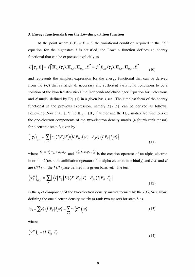
3. Energy functionals from the Löwdin partition function

At the point where f (E) = E = Ei the variational condition required in the FCI

equation for the eigenstate i is satisfied, the Löwdin function defines an energy

functional that can be expressed explicitly as

(10)

and represents the simplest expression for the energy functional that can be derived

from the FCI that satisfies all necessary and sufficient variational conditions to be a

solution of the Non Relativistic-Time Independent-Schrödinger Equation for n electrons

and N nuclei defined by Eq. (1) in a given basis set. The simplest form of the energy

functional in the previous expression, namely E[γ1, E], can be derived as follows.

Following Roos et al. [17] the HI,II = (HII,I)T vector and the HII,II matrix are functions of

the one-electron components of the two-electron density matrix (a fourth rank tensor)

for electronic state L given by

Lγ2( )

ij,kl= cI

LI Eij K K Ekl J cJ

L −δ jkcILI Eil J cJ

L

I ,J ,K

∑ (11)

where and is the creation operator of an alpha electron

in orbital i (resp. the anihilation operator of an alpha electron in orbital j) and I, J, and K

are CSFs of the FCI space defined in a given basis set. The term

(12)

is the ij,kl component of the two-electron density matrix formed by the I,J CSFs. Now,

defining the one electron density matrix (a rank two tensor) for state L as

Lγ1= c

I

LI E

ijJ c

J

L

I ,J

∑ = cI

L γ1

IJ( )ijcJ

L

I ,J

∑ (13)

where

(14)

E γ1,E[ ] = f HI ,I (γ 1),HI ,II ,HII ,II ,E⎡⎣ ⎤⎦ = f EHF (γ 1),HI ,II ,HII ,II ,E⎡⎣ ⎤⎦

Eij= a

iα+ajα−+ a

iβ+ajβ− a

iα

+ (resp. a

jα

−)

γ2

IJ( )ij,kl

= I Eij K K Ekl J −δ jk I Eil J⎡⎣ ⎤⎦K

∑

γ1

IJ( )ij= I E

ijJ

9

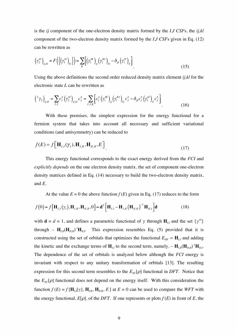
is the ij component of the one-electron density matrix formed by the I,J CSFs, the ij,kl

component of the two-electron density matrix formed by the I,J CSFs given in Eq. (12)

can be rewritten as

γ2

IJ( )ij,kl

= F γ1

IJ( )kl

{ }( ) = γ1

IK( )ijγ1

KJ( )kl

−δ jk γ1IJ( )

il

K

∑. (15)

Using the above definitions the second order reduced density matrix element ij,kl for the

electronic state L can be rewritten as

Lγ2( )

ij,kl= cI

L γ2

IJ( )ij,klcJL

I ,J

∑ = cIL γ

1

IK( )ijγ1

KJ( )klcJL −δ jkcI

L γ1

IJ( )ilcJL

I ,J ,K

∑. (16)

With these premises, the simplest expression for the energy functional for a

fermion system that takes into account all necessary and sufficient variational

conditions (and antisymmetry) can be reduced to

. (17)

This energy functional corresponds to the exact energy derived from the FCI and

explicitly depends on the one electron density matrix, the set of component one-electron

density matrices defined in Eq. (14) necessary to build the two-electron density matrix,

and E.

At the value E = 0 the above function f (E) given in Eq. (17) reduces to the form

f 0( ) = f HI ,I γ1( ),HI ,II,H

II ,II, 0 = d

TH

I ,I−H

I ,IIH

II ,II( )−1H

II ,I

d (18)

with d = d = 1, and defines a parametric functional of γ1 through HI,I and the set {γ1

IJ}

through – HI,II(HII,II)-1HII,I. This expression resembles Eq. (5) provided that it is

constructed using the set of orbitals that optimizes the functional EHF = HI,I and adding

the kinetic and the exchange terms of HI,I to the second term, namely, – HI,II(HII,II)-1HII,I.

The dependence of the set of orbitals is analyzed below although the FCI energy is

invariant with respect to any unitary transformation of orbitals [13]. The resulting

expression for this second term resembles to the EXC[ρ] functional in DFT. Notice that

the EXC[ρ] functional does not depend on the energy itself. With this consideration the

function f (E) = f [HI,I[γ1], HI,II, HII,II, E ] at E = 0 can be used to compare the WFT with

the energy functional, E[ρ], of the DFT. If one represents or plots f (E) in front of E, the

f (E) = f HI ,I (γ 1),HI ,II ,HII ,II ,E⎡⎣ ⎤⎦

10

energy of any DFT method should be located on the vertical axis f (0). The reason, as

noted above, is because the EXC[ρ] of any DFT method is equivalent to the second term

of the f (0) Löwdin function where in this case E does not appear explicitly in the

function as occurs in DFT. So far it seems the most licit and appropriated way to

compare both models, namely, the WFT, also so-called ab initio methods, and the DFT.

The functions representing both theories, namely, E[ρ] in Eq. (5) and the Löwdin

function f (E) at E = 0 from Eq. (9) are equivalent if they are build using the same basis

set with the same external potential v(ri;R1; ··· ;RN), the same number of electrons, n,

and in addition in DFT the set of orbitals is the KS while in WFT is HF. With these two

premises the comparison is well established and permitted.

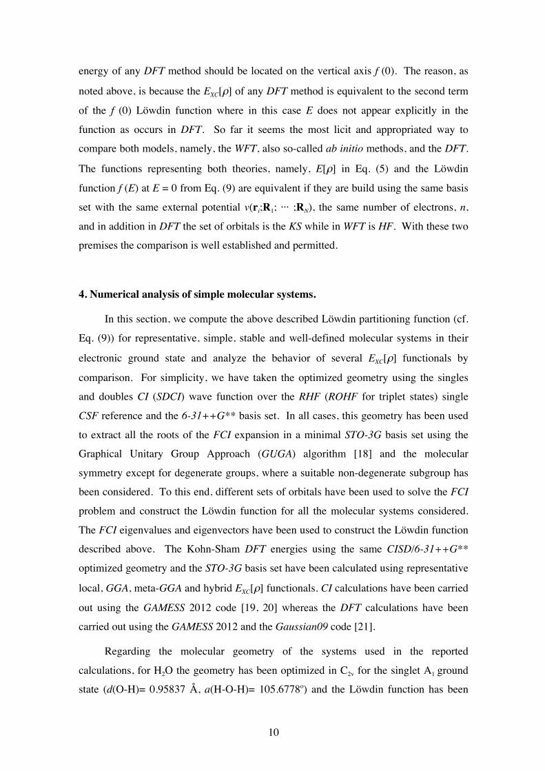
4. Numerical analysis of simple molecular systems.

In this section, we compute the above described Löwdin partitioning function (cf.

Eq. (9)) for representative, simple, stable and well-defined molecular systems in their

electronic ground state and analyze the behavior of several EXC[ρ] functionals by

comparison. For simplicity, we have taken the optimized geometry using the singles

and doubles CI (SDCI) wave function over the RHF (ROHF for triplet states) single

CSF reference and the 6-31++G** basis set. In all cases, this geometry has been used

to extract all the roots of the FCI expansion in a minimal STO-3G basis set using the

Graphical Unitary Group Approach (GUGA) algorithm [18] and the molecular

symmetry except for degenerate groups, where a suitable non-degenerate subgroup has

been considered. To this end, different sets of orbitals have been used to solve the FCI

problem and construct the Löwdin function for all the molecular systems considered.

The FCI eigenvalues and eigenvectors have been used to construct the Löwdin function

described above. The Kohn-Sham DFT energies using the same CISD/6-31++G**

optimized geometry and the STO-3G basis set have been calculated using representative

local, GGA, meta-GGA and hybrid EXC[ρ] functionals. CI calculations have been carried

out using the GAMESS 2012 code [19, 20] whereas the DFT calculations have been

carried out using the GAMESS 2012 and the Gaussian09 code [21].

Regarding the molecular geometry of the systems used in the reported

calculations, for H2O the geometry has been optimized in C2v for the singlet A1 ground

state (d(O-H)= 0.95837 Å, a(H-O-H)= 105.6778o) and the Löwdin function has been

11

calculated using this geometry and FCI/STO-3G singlet wave functions of A1 symmetry

generated using the GUGA algorithm (N(FCI) = 70 CSF's) using the HF orbitals. We

proceed similarly for SH2 (A1 ground state in C2v symmetry with d(S-H) = 1.33088 Å,

a(H-S-H) = 92.9297o; N(FCI) = 382 CSF's), CH4 (singlet A1 ground state optimized in

C2v (d(C-H) = 1.08527 Å, a(H-C-H) = 109.4712o; N(FCI) = 1436 CSF's), NH3 (singlet

A’ ground state optimized in Cs (d(N-H)= 1.00967 Å, a(H-N-H)= 107.9010o; N(FCI) =

616 CSF's), NH4+( singlet A1 ground state optimized in C2v (d(N-H)= 1.01972 Å, a(H-

N-H)= 105.6778o; N(FCI) = 1436 CSF's).

We also included two molecules having a triplet ground state: CH2 (triplet B1

ground state optimized in C2v (d(C-H)= 1.07593 Å, a(H-C-H)= 132.3511o; Löwdin

function calculated using this geometry and FCI/STO-3G triplet wave functions of B1

symmetry with N(FCI) = 148 CSF's) and O2 (B1g ground state optimized in D2h (d(O-

O)= 1.2215 Å); Löwdin function calculated using this geometry and FCI/STO-3G

singlet wave functions of B1g symmetry with N(FCI) = 106 CSF's).

In Table 1 we report a set of WFT and DFT energy values for the set of simple

molecules described above for which the Löwdin function defined in Eq. (9) has been

constructed using the FCI results in a STO-3G minimal basis set. Here we report the

energy of the systems (same n, same external potential v(ri;R1; ··· ;RN), and same basis

set) obtained using HF and several standard parameterizations of the EXC[ρ] functional

for LDA [22, 23], GGA (PW91PW91 [24], BLYP [25, 26], and PBEPBE [27]), meta-

GGA (revTPSS [28], PKZBPKZB [29], and VSXC [30]) and hybrid (B3LYP [26, 31] and

PBE0 [32]). It should be emphasized that exactly the same FCI energies are obtained

using different orbitals to construct the FCI space as expected from the fact that the

same atomic basis set is used in all the cases.

In Table 2, we provide some relevant values for the Löwdin functions

constructed from the FCI matrix using different sets of orbitals to analyze the

dependence of the H11 and the f(0) values on the set of basis fuctions used to solve the

FCI problem. In particular, we have used the RHF/ROHF set of orbitals (orbital basis

set A), symmetrized Huckel orbitals (orbital basis set B), the Kohn-Sham orbitals from

S-VWN [22, 23] LDA functional (orbital basis set C), BLYP [25, 26] GGA functional

(orbital basis set D) and the PBE0 [32] hybrid functional (orbital basis set E). Finally,

we also used the natural orbitals corresponding to the FCI ground state to show the

12

relevance of the exact one electron density matrix in defining the wave function of the

ground state (orbital basis set F).

In all cases, the Löwdin function f (E) for the present systems has the general

structure shown in Figure 1 with the corresponding value of K (dimension of the FCI

matrix). For the minimal basis set, all electronic states are bound (i.e.: Ei < 0 for i = 1,

K with K = N(FCI)) and, hence, the value f (0) appears after the last vertical asymptote

(aK). However, for a general case the f (0) value can be located between two vertical

asymptotes ai and ai+1. This fact does not have any relevant consequence for the

discussion below. We note that each vertical asymptote ai is an eigenvalue of the HII,II

matrix. In the present case we have only K–1 vertical asymptotes because this is the

dimension of the HII,II matrix if the dimension of the full H is K = N(FCI). When the E

variable takes a value E = ai then f (E) function goes to infinity at this point. The f (E)

function is a non-increasing function of E. Finally we recall that as E tends to ±∞ then f

(E) goes to HI,I = H11 = Eref. In this case, each branch located within two consecutive

vertical asymptotes, lets say, ai and ai+1, cuts the straight line f (E) = E one time and only

one. This straight line passes through the point (0, 0). The point where a branch cuts

the straight line is an eigenvalue of the full H matrix. The last branch cuts the straight

line f (E) = E at the point E = EK corresponding to the highest eigenvalue of this matrix,

and also cuts the vertical axis f (0) and from this point it goes to Eref as E tends to +∞.

The f (E) function when E tends to ±∞ takes the values Eref (which corresponds to EHF

when the HF orbitals are used (orbital set A), and to the expectation value of the

Hamiltonian using the Huckel determinant, the KS determinant or the natural

determinant for the ground state (orbital sets B to F)). In other words,

= H11 = Eref. All these features show that the overall behavior of the calculated Löwdin

function throughout the whole E horizontal axis is well defined.

Regarding the particular values of the energies for the systems reported in Table

1, we emphasize that for each system the same number of electrons n, the same external

potential v(ri;R1; ··· ;RN), and same basis set has been used to obtain the energy using

the FCI, HF and several standard parameterizations of the EXC[ρ] functional. For all

the systems described above, the HF energy is always above the exact FCI energy, as

known from the variational nature of the wave function expressed in terms of CI

expansions. In general, the DFT energies obtained using the selected functionals show

limE→±∞

f E( ) =HI ,I

13

important differences depending on the particular form of the exchange-correlation

functional considered. The LDA approach provides a value of the energy of the ground

state that is above the exact FCI energy value. A detailed analysis of the values

reported in Table 2 shows that the Löwdin function has essentially the same form but

shows a the dependence of the H11 and the f(0) values on the set of basis fuctions used to

solve the FCI problem. The expected values of the energy H11 = Eref using the sets of

orbitals C to F are slightly above the HF energy, whereas a larger difference is observed

when using the symmetrized Huckel orbitals. This is in line with the fact that the HF

determinant provides the lowest variational energy using a single determinant

description. Interestingly enough, the LDA energy value is also above the HF energy

and close to the value of the branch of the Löwdin function that cuts the f (E) axis at E =

0. However, the GGA, meta-GGA and hybrid DFT energy values are all below the exact

FCI value. As a general rule, the differences between energy values provided by the

GGA, meta-GGA and hybrid DFT functionals are system dependent and larger for

systems with larger number of electrons. A similar picture of the Löwdin function is

obtained using different basis sets with a small variation of the f (0) value (except

perhaps when using the roughly approximated symmetrized Huckel basis set). Also, a

significant change of the weight of the reference determinant in the ground state is

observed for the differents orbital sets, with the larger value obtained using the natural

orbitals of the FCI ground state. This value provides an estimation of the contribution

of the one electron density matrix to the FCI wave function.

In view of the previous discussion, the equivalence between E [ρ] and the

expression of the Löwdin function at E = 0 provides an argument to explain this

dispersion of results in terms of the complexity of the particular functional (larger

number of parameters leads to lower energy) and the lack of variationality with respect

to E. This comparison model suggests that the present DFT approaches require a

revision to include an additional variational term in addition to the density ρ (r), playing

the role that the variable E plays in the Löwdin function. From this comparison scheme

it is clear that the variable E controls the variational requirements in order to achieve a

consistent description of the molecular electronic structure of both ground and excited

states. The lack of an explicit dependence on E in current DFT based approaches (along

with the difficulties to treat open shell states) explains the limitations of this theory to

describe excited states. Finally, this formal mathematical correspondence also suggests

14

that DFT functionals can be seen as effective single determinant approaches in the sense

used by Clementi and coworkers to define their semi-empirical density functional

approximations to obtain correlation energies from HF wave-functions [33].

5. Conclusions

The results exposed in the previous sections reveals that the Löwdin function of

Eq. (9) provides a tool of comparison model between the wave function and the density

functional theories. This model provides an explicit form of the exact energy functional

for a fermion system and reveals the inherent structure of both theories in order to be

compared. The DFT functionals can be seen as special cases of Löwdin function that

do not satisfy all necessary and sufficient conditions on ρ (r). The latter implies that,

if we are given any density function ρ (r) which are not correctly derivable from a spin

and space symmetry adapted wave function, there will always exist at least a functional

which is capable of detecting this fact, in the sense that ρ (r) will yield to an energy for

this functional which is lower than its minimum energy. Ignoring the type of

restrictions imposed by the spin and space symmetry adapted when making a variational

calculation on such a system leads to an energy minimum that will exhibit the

phenomenon of "overcorrelation". That is, the correlations expressed by the ρ (r)

function will be inconsistent with a γ1(r1;r1') function derivable from a spin and space

symmetry adapted wave function , even for a closed-shell system.

From this analysis, the increasing empiricism in defining current EXC based on the

statistical performance is clearly limited by the form of the exact energy functional.

Extension of DFT to include the dependence with E to restore variationality may

improve existent functionals to describe the ground and excited states.

Acknowledgements

Financial support has been provided by the Spanish Ministerio de Economía y

Competitividad (formerly Ministerio de Ciencia e Innovación) through grants

CTQ2011-22505 and FIS2008-02238) and by the Generalitat de Catalunya through

grants 2009SGR-1472, 2009SGR-1041 and XRQTC. Part of the computational time

Ψ(r1s1,,r

nsn)

15

has been provided by the Centre de Supercomputació de Catalunya (CESCA) which is

also gratefully acknowledged.

16

Figure 1. Qualitative representation of the Löwdin function f (E) for a FCI problem

with K = 8 CSF's and H11 = Eref, to show the general behaviour of this function. In this

example, the horizontal assimptote corresponds to Eref (i.e. single configuration

representations: RHF for closed shell systems, ROHF or GVB for open shell singlets

and triplets). The points E1 ≤ E2 ≤ E3 ≤ ... ≤ E8 correspond to the set of eigenvalues of

the full H matrix of dimension K = 8 (i.e.: those in which f (E) = E). The K - 1 = 7

vertical assimptotes a1 ≤ a2 ≤ a3 ≤ ... ≤ a7 correspond to the eigenvalues of the K - 1

reduced H matrix, namely, HII,II. See text for more explanation details of this plot.

17

Table 1. Relevant energy values for the FCI energies and energies of representative

EXC[ρ] functionals. In all cases, the basis set is STO-3G and the geometries correspond

to CISD/6-31++g** optimised structures (see text for details). The same sets of FCI

eigenvalues are obtained independently of the orbitals used to construct the

determinants discussed in Table II.

H2O NH3 SH2 CH4 NH4

+ CH2 O2 K = N (FCI) 70 616 382 1436 1436 148 106 E1 -75.012114 -55.517543 -394.354092 -39.805451 -55.946702 -38.472608 -147.747895 E2 -74.419386 -54.989548 -393.780008 -38.973091 -55.099684 -37.943644 -147.146834 E3 -74.015740 -54.931878 -393.610959 -38.917079 -55.065056 -37.888937 -146.901982 ... EK-1 -28.052661 -16.773511 -179.589921 -9.0789790 -13.342182 -11.697235 -103.312082 EK -27.401570 -16.607329 -177.750980 -8.9003961 -13.139050 -11.366848 -101.543057 E(HF/ROHF) -74.962674 -55.453330 -394.311615 -39.726846 -55.866554 -38.429892 -147.632382 E(SVWN5) -74.731653 -55.289280 -393.511068 -39.616730 -55.709647 -38.235051 -147.197578 E(PW91PW91) -75.278919 -55.752563 -394.908835 -40.006167 -56.167937 -38.617965 -148.238832 E(BLYP) -75.277026 -55.744244 -394.899925 -39.994248 -56.157526 -38.614300 -148.245053 E(PBEPBE) -75.225100 -55.706750 -394.755311 -39.966679 -56.123036 -38.581657 -148.141707 E(revTPSS) -75.326254 -55.796958 -394.970071 -40.051700 -56.210114 -38.666296 -148.328874 E(PKZBPKZB) -75.193024 -55.688394 -394.529979 -39.958448 -56.104226 -38.573009 -148.079450 E(VSXC) -75.349301 -55.814583 -395.109922 -40.059908 -56.228813 -38.668603 -148.359499 E(PBE0) -75.245260 -55.725543 -394.816928 -39.984130 -56.141393 -38.599394 -148.155159 E(B3LYP) -75.312120 -55.784317 -394.951857 -40.038517 -56.197663 -38.646414 -148.273295