Remote Sensing and GISApplications for Hilly Watersheds

SUBASHISA DUTTA DEPARTMENT OF CIVIL ENGINEERING

IIT GUWAHATI

Deciding Alternative Land Use Options in a Watershed Using GIS

2Source: Anita Prakash et al, 2007

High Resolution of IRS-P6 Imagery

VIENNA

3Source: NRSC website

High Resolution of CARTOSAT-2 Imagery

4Part of Varanasi, Uttar Pradesh, India Source: NRSC website

Topics to be coveredTopics to be covered

• Hydrological response of a hillslope under• Hydrological response of a hillslope under

extreme rainfall events

• GIS as a tool for watershed management

• Analysis of digital elevation model ( terrain

data))

• Case studies and discussion

5

The Hydrologic Cycle at hillslope

6Physical Processes Involved in Runoff Generation

Hillslope HydrologyHillslope HydrologyCritical Hydrologic Processes

InfiltrationOverland FlowSubsurface StormflowSubsurface StormflowSoil Macropores and Water Flow

Consequences :Flash FloodinggSlope Failures and SlidesSoil Erosion

7

Debris FlowGroundwater Pollution

Hillslope Experimental Plot

Geographic Location - 26°12′ N latitude and 91°42′ EGeographic Location 26 12 N latitude and 91 42 E longitude

T h8

Topography – Average slope 20%, COV 10.49% Microtopographic variation not significant

Hillslope Experimental Setup

UPSTREAM CHANNELPROFILE PROBE LOCATION

Upper Channel

SIDE PLATES

OVERLAND

VENTURIMETER

VALVE

LOCATION

18 mPiezometer

Side Plate

DOWNSTREAM CHANNEL

OVERLANDFLOW

PUMPPUMP

Piezometer

PONDMEASURING

TANKOUTLET

Lower Channel

6 m

Extreme Storm Intensity – about 50 - 400 mm/hr

9

mm/hrStorm Durations – 15 -120 minutes

10

Overland Flow - Results6

3

4

5

entra

tion,

t c(m

in) Sparse

Moderate

Dense

0

1

2

Tim

e of

Con

ce

Outflow hydrographFig. 5

00 100 200 300 400 500

Equivalent Rainfall Intensity, i (mm/hr)Fig. 6Relationship between tc and i

300Sparse

Similar response in sparse and moderrate vegetationSimilar macropore network150

200

250

n R

ate,

f b (m

m/h

r)

SparseModerateDense

Distinct changes in behavior in dense vegetationSignificant change in macropore 0

50

100

0 100 200 300 400 500

Infil

tratio

n

11

connectivity and network0 100 200 300 400 500

Equivalent Rainfall Intensity, i (mm/hr)Fig. 7Relationship between fb and i

At t 22 iInitial state

Temporal dynamics of subsurface storm flow

At t=22minAt t=18min.Initial state

At t=42 rainfall ceased At t=51min.At t=29 min.

At t=42 rainfall ceased At t 51min.

12

Temporal dynamics of subsurface storm flow ( Continued)

At t=66min. At t=85 min. At t=99 min.

C i i l Ob iCritical Observations :

1. Fast subsurface stormflow ( within 1-2 hours of the storm event)

2. Initiation of subsurface storm flow occurs for even a storm event of 50 mm/hr

3 T ll h d t t bl f ti th b d k

13

3. Temporally perched water-table formation on the bed-rock

Saturation in zones of convergent topographyp g p y

Hydrological effect of land use/land cover changey g g

• Change in top soil macroporosity, more likely to have overland flowgeneration

• Blocking of subsurface stormflow path, more concentrated flowgeneration, leading high sheet erosionB i th h ld fl h i it i t ll d b i f ll i t it• Being a threshold flow mechanism, it is controlled by rainfall intensity,vegetation condition, soil layers

• Wetness index, based on DEM, predicts the subsurface storm flowpathspaths

• Identification of “Hotspots” in a hilly watershed, related to flash floodsand soil erosion, sediment transport capacity and natural sedimenttrapper

• Land use/land cover planning to be carried out by integrating“hydrological knowledge” on geospatial database

17

18

Why GIS?

C h dl hi ll f d d tCan handle geographically referenced data or spatial data as well as non-spatial data

Can handle relational numerical expressions between these data sets

Ideal for natural resource management

19

B i F ti f GISBasic Functions of GIS

Capturing dataStoring dataManipulating dataRetrieving and Querying dataRetrieving and Querying dataAnalyzing dataDi l i d tDisplaying data

20

Data TypesSpatial Data Non-spatial Data

TopographyLand Use Land Cover S il

Descriptive Attributes

Soil TypeSoilWater bodiesState District Blocks

Soil TypeLand Use TypeVillage Name

State, District, BlocksVillagesForests

Street Name

ForestsGeologyRoad Network

21

Representation of Spatial Data

22

23

Spatial Data Models

Vector Data Model Raster Data Model

Based on geometry of Digital RepresentationG id C ll

Pointas Grid Cells

Satellite Images

Line

P l

Aerial Photographs

Polygon Digital Elevation Models (DEM)

24

Vector and Raster Data Model

25

Vector Data ModelB i hi l fArc-Node data structure Basic graphical features

Point Line Polygon

26

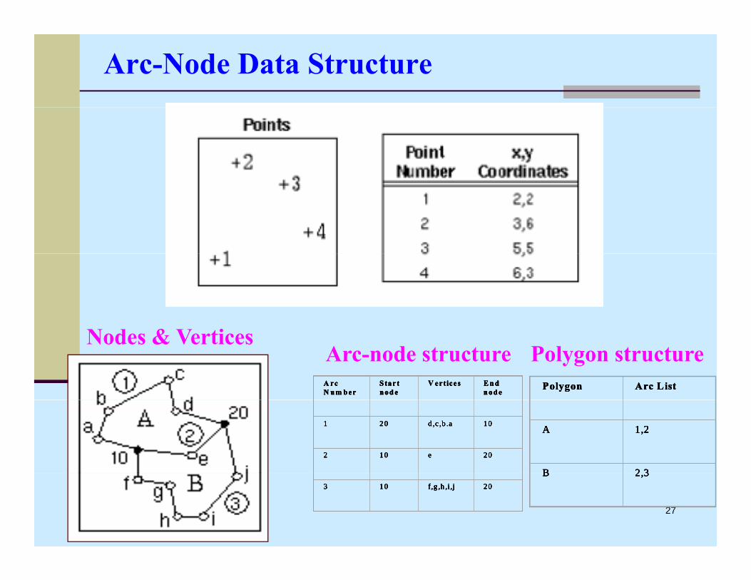
Arc-Node Data Structure

Polygon Arc ListPolygon Arc ListPolygonPolygon Arc ListArc ListA rc N u m b e r

S ta r t n o d e

V ertices E n d n o d e

A rc N u m b e r

S ta r t n o d e

V ertices E n d n o d e

A rc N u m b e rA rc N u m b e r

S ta r t n o d eS ta r t n o d e

V erticesV ertices E n d n o d eE n d n o d e

Nodes & VerticesArc-node structure Polygon structure

A 1,2

B 2 3

A 1,2

B 2 3

AA 1,21,2

BB 2 32 3

1 2 0 d ,c ,b .a 10

2 1 0 e 20

1 2 0 d ,c ,b .a 10

2 1 0 e 20

11 2 02 0 d ,c ,b .ad ,c ,b .a 1010

22 1 01 0 ee 2020

27

B 2,3B 2,3BB 2,32,33 1 0 f,g ,h ,i,j 203 1 0 f,g ,h ,i,j 2033 1 01 0 f,g ,h ,i,jf,g ,h ,i,j 2020

Topology : Defining Spatial Relationships

Three major topological concepts:

Connectivity: Arcs connect to each other at nodes.

Area definition: Arcs that connect to surround d fi lan area define a polygon

Contiguity: Arcs have direction and left and i ht idright sides

28

Connectivity

29

Area Definition

30

Contiguity : Adjacency

31

Vector Data Model

Points: represent discrete point features

each point locationhas a record in thetable

airports are point featuresh i t i t d

32

each point is stored as a coordinate pair

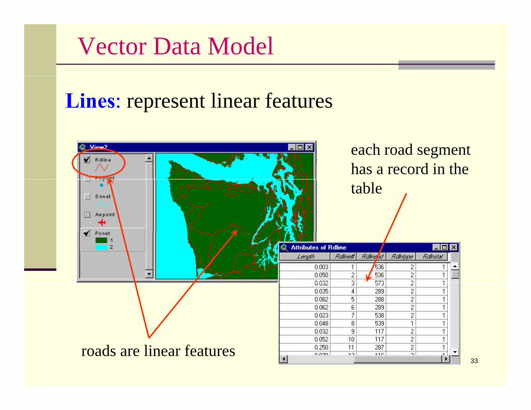
Vector Data Model

Lines: represent linear features

each road segmenthas a record in thetable

33roads are linear features

Vector Data Model

Polygons: represent bounded areas

each bounded polygonhas a record in thetable

polygonal features

34

polygonal features

Multiple Layers of Vector Data

35

Data Structures

“where” of GIS is determined by coordinatewhere of GIS is determined by coordinate (map) data structures, but …

“what” of GIS is determined by tabular (relational database) data structures( )

GIS Database = Coordinate data + Attribute Data

36

Attribute Data Structures

Attribute data are stored in database tables.

Tables are composed of:

Fi ldFields

andand

Records

37

Use of Tabular Data

Making queries

Promoting and sorting recordsPromoting and sorting records

Displaying selected sets

Modifying selected sets

Basic descriptive statisticsBasic descriptive statistics

38

Making Queries

Selecting records from tables/features

39

Displaying Selected Sets

Selecting records from tables also select features from themesfrom themes

40

Analysis Tools of GIS

BUFFER ANALYSIS

OVERLAY ANALYSIS

NETWORK ANALYSIS

41

Buffering

Quantifying a spatial entity to influence its neighbours or the neighbours to influence the character of aor the neighbours to influence the character of aSpatial entity

Point

Line

Polygon42

Polygon

POINT BUFFER

43

LINE BUFFER

44

Overlay Analysis

Point over Polygon

45Line over Polygon

Overlay Operators

46

Analysis of DEM for extraction of Watershed yparameters

47

Digital Elevation ModelsRemotely Sensed Satellite ImagesDigital Elevation Models (DEM)

Raster Data Structure

48

DEM Data from Contours

Contours720 720

Contours740

720

700

680

49680700720740

DEM ElevationsContours

700

680

50

A Simple Digital Elevation Model

67 56 49 46 50

cell size

53 44 37 38 4850

(cell value)58 55 22 31 24

61 47 21 16 19

(cell value)

12 11 123453 cell

51

DEM Data Sources

1 km DEM of the earth (GTOPO)

100 m DEM from 1:250,000 scale maps

30 m DEM from 1:24,000 scale map, p

90 m Shuttle Radar Topography Mission (SRTM)p g p y ( )

52

Using DEM Data

1 1Direction of Steepest Descent

67 56 49 67 56 49

53 44 37 53 44 37

58 55 22 58 55 22

26.1624467

=−

141

5367=

−Slope:

53

2 1

Eight Direction Pour Point Model

32 64 128

16 116

8 4

1

28 4 2

54

Flow Direction Grid

2 2 4 4 8

1 2 4 8 4

128 1 2 4 8

2 1 4 4 4

1 2 1611

55

30 Meter DEMEle ations in metersElevations in meters ftp://ftp.tnris.state.tx.us/tnris/demA.html

56

Flow Direction Grid

32 64 128

16

8 4

1

2

57

Fl N kFlow Network

58

Flow Accumulation Grid

0 0 000 0 0 00 0

0

0 0

03 2 2

1

0

0 0

0

0

3 2 2

11 1

00

0 0

0

011 1

1 15

0

0

0

0 0

011 1

1 15

0 2 524 1 0 12 245

59

Fl A l i 5 C ll Th h ldFlow Accumulation > 5 Cell Threshold

St Li

0 0 00 0

Stream Lines

0

0 03 2 2

0 0 011 1

0

0

0 01

12

15

245

60

0 2 245

St N t k f 5 ll Th h ldStream Network for 5 cell Threshold Drainage Area

0 0 000

0

0

03 2 2

00

0 00

111

1 0

0

0 0 115

2 5 161

024

1

Watershed Outlet

62

Watershed Draining to the Outlet

63

SRTM Data Source Website: http://srtm.csi.cgiar.org/

64

SRTM Data Selection Option

65

Sample DEM Data

66SRTM Data: 90 m Resolution

Computing Flow Direction

67Flow Direction Map

Flow Accumulation from Raw DEM

Discontinuous Flow Lines orLoopsLoops

Sinks

Filling is Required

68

Sink Filling

C ti St Li

69

Continuous Stream Line

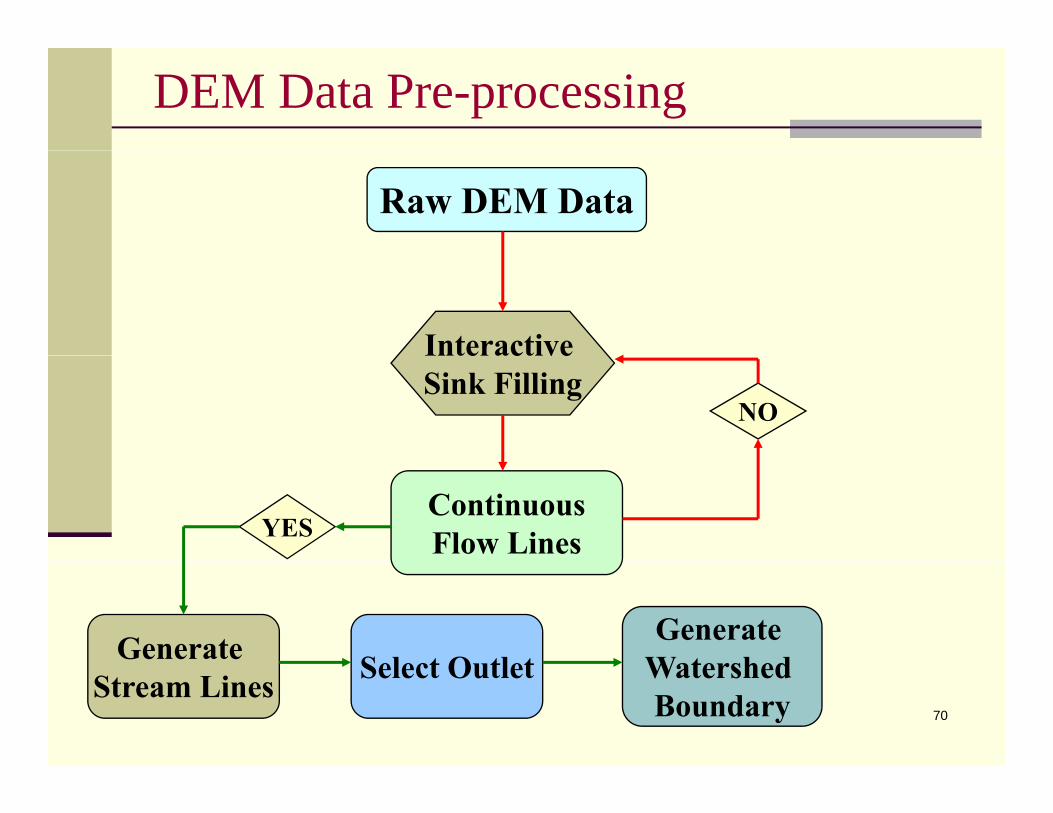
DEM Data Pre-processing

Raw DEM Data

InteractiveInteractive Sink Filling

NO

ContinuousFlow LinesYES

Generate Select O tletGenerate

Watershed70

Stream Lines Select Outlet Watershed Boundary

Filled DEM Data

71

Stream Network from Filled DEM

72

Defining Watershed Boundary

Watershed Boundary

Outlet

73

Case studies : GIS and RS applications

74

Case study : Shiwalik hill in DehradunDEM t CARTOSAT iDEM : stereo CARTOSAT imagery

Wetness index image Ln(As/S) Stream power index (A *S) Sediment transport index

75Source: suresh kumar et al, 2008, ISRS-36, 159-165

Case study-2: Spatial distribution of annual sediment yield estimation

Source: Manish and Suresh

76Study area: Jhikhu Khola watershed in NEPAL

Conclusion and DiscussionsExtreme hydrological response of a hillslope :

discussed, their prediction based on wetness index,, p ,

their knowledge for land use/land cover planning

GIS: introduced its use in watershed managementGIS: introduced, its use in watershed management

Digital elevation model: extraction of watershed

parameters, wetness index, stream power index

Recent case studies using high-resolution DEM andg g

satellite remote sensing

77

Th k YThank You

78