ISWS CR 165 Loan c. 1

REMOTE SENSING OF CROP HAIL DAMAGE

BY

Neil G. Towery, John R. Eyton, Stanley A. Changnon, Jr. and Christine L. Dailey

Report of Research Conducted 15 May 1974 - 14 May 1975

FOR

The Country Companies

July 21, 1975

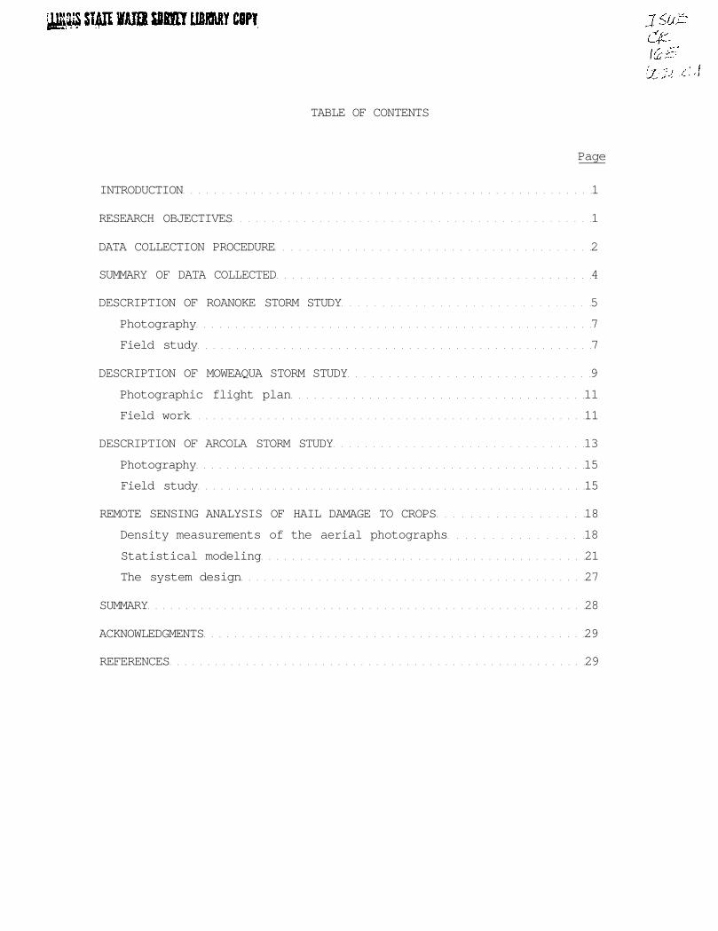
TABLE OF CONTENTS

Page

INTRODUCTION 1

RESEARCH OBJECTIVES 1

DATA COLLECTION PROCEDURE 2

SUMMARY OF DATA COLLECTED 4

DESCRIPTION OF ROANOKE STORM STUDY 5 Photography 7 Field study 7

DESCRIPTION OF MOWEAQUA STORM STUDY 9 Photographic flight plan 11 Field work 11

DESCRIPTION OF ARCOLA STORM STUDY 13 Photography 15 Field study 15

REMOTE SENSING ANALYSIS OF HAIL DAMAGE TO CROPS 18 Density measurements of the aerial photographs 18 Statistical modeling 21 The system design 27

SUMMARY 28

ACKNOWLEDGMENTS 29

REFERENCES 29

INTRODUCTION

Crop disease studies (Jackson, 1970; Philpott et al., 1969) have used color and infrared films to detect damage to crops from various forms of stress. These studies basically revolve around damaged crops reflecting differently in certain wavelengths (through changes in chlorophyll production) and being detected by the film. These studies seem to suggest that hail damage could also be detected through the same process-damaged crops reflect radiation differently. Thus, a study (Changnon et al., 1970) was conducted in 1969 to investigate this possibility. This study on one storm in July and test plots at Western Illinois University concluded that visual inspection and densitometer measurements could estimate the damage with reasonable accuracy. Both normal color and infrared films were used with little difference in the accuracy of assessing the hail damage. Further study was recommended but not performed because of lack of funding.

In April 1975 initial discussions began with the Country Companies concerning initiating and expanded project. A letter describing the possible project was submitted to the Country Companies on April 17, 1974, and a formal agreement followed after negotiations and approval from Country Companies staff. The final formal agreement was submitted on May 15, 1974 after receipt of approval (May 1, 1974) from the Country Companies. The contract was signed on May 29, 1975.

A separate contract to provide the aerial photography was arranged between the Country Companies and Danner and Associates, Inc. of Urbana. The photography by Danner and Associates was to be done under the direction of the Illinois State Water Survey. Danner and Associates handled the entire photography portion from purchase of the film flight mission, and having the film processed by Mead Techniques, Inc. of Dayton, Ohio.

The objectives of the project appear in the next section, followed by a detailed description of the data collection, both airborne and at the surface. Then, the 3 major storms studied are each described in detail, followed by discussion of the film analysis procedure and then a summary and recommendations.

RESEARCH OBJECTIVES

The main objective was to investigate the application and potential accuracy of using aerial photography to assess hail damage to Illinois' major crops (corn, soybeans, wheat). A secondary objective was to investigate aerial photography as a means to quickly delineate severe crop damage areas so as to help direct surface storm surveying operations. In each case, development of a technology for direct application to hail insurance needs was the ultimate goal.

-2-

These objectives required that aerial photography (at various times after the storms and at various altitudes) be taken of crops damaged by hail during 5 or 6 separate storms at different stages of growth of the various crops throughout the growing season (15 May-30 September 1974). The photographic data were to be compared with standard crop damage assessments made by an adjustor from the Country Companies.

The plan was to compare the collected aerial photography data and crop loss data to determine if any relationship existed. These comparisons were to be done for each surface crop loss assessment. Hopefully, the accumulation of these comparisons throughout the crop growing season would be sufficient to determine possible relationships so as to determine the feasibility of crop loss assessment using aerial photographs.

DATA COLLECTION PROCEDURE

The information about the occurrence of crop damaging hailstorms for potential studies usually came from the Country Companies. After it was determined that a hailstorm might meet the general guidelines for a photographic mission, the storm was quickly inspected by the crop adjuster and Illinois State Water Survey (ISWS) personnel. The general guidelines used were 1) that crop damage range from 0% to greater than 60%, and be concentrated in a relatively small area (usually less than 4 square miles), and 2) that the storm area must contain different growth stages of each crop. If the storm met those requirements, Danner and Associates were notified of the area to be photographed, the altitudes from which the photography was to be taken, the film types to be used, and the direction of the flight lines. The first photographic mission for a particular storm was performed the first day weather permitted after the storm, and in all storm cases studied, the flights were always completed within the desired 6-14 days after the storm occurrence date.

Table 1 presents the relationship between flight altitude above ground level (AGL) and amount of area covered per photograph using stereo photography, which was used during this project. For instance, at 3,000 ft AGL each photograph covers a gross area of .726 square miles or 465 acres. The net area covered for stereo photography (which allows easy identification of hills and valleys) is .204 square miles or 130 acres. This Table also demonstrates the value of increasing the flight altitude. If the altitude is increased to 6,000 ft AGL the area covered is four times as great. This would represent a considerable savings in photographic cost because only one fourth as many photographs are needed to cover the same area.

The photographic missions require more than normal flying expertise for quality photography. The pilot must be able to fly the aircraft along a straight line called the flight line. This is often difficult at times on days with high or gusty winds.

-3-

Table 1. Flight Altitudes and Their Relationship to the Photographic Transparency Characteristics.

Altitude Transparency Area Covered AGL* Scale Square Miles Acres Feet 1" = ft. Net** Gross Net** Gross 600 100 .008 .029 5.2 18.60 1200 200 .032 .113 21 74 1500 250 .050 .182 32.5 116 3000 500 .204 .726 130 465 6000 1000 .814 2.90 521 1,860 7920 1320 1.42 5.06 907 3,200 9000 1500 1.83 6.54 1,171 4,184 12000 2000 3.25 11.60 2,083 7,438 15000 2500 5.08 18.16 3,254 11,622 * AGL - Above Ground Level ** Using Stereo Photography (60% forward overlap - 30% sidelap)

After the photographic mission was completed, Danner and Associates sent the film to be processed. The film was processed in such a manner that the film transparencies could be developed almost immediately, but prints took longer. The entire process nominally took 14-21 days. Because of this approximate 2-3 week delay, a camera malfunction on the second photographic mission was not discovered for almost 3 weeks after the first mission. Therefore, the film processing procedure was changed slightly after that flight. The new procedure required that the transparencies be processed, returned to the Illinois State Water Survey for inspection, and then returned to the processor for processing of the prints. This caused a further delay in receipt of the prints, but served the purpose of insuring that the quality of the photography was good, another mission could be done within a week of the first flight.

The time elapsed between the storm occurrence and receipt of processed prints was similar to the normal waiting period before field adjustments begin. Thus, it was possible to use aerial prints as an aid in selection of fields for adjustment.

John Williams, the adjustor assigned to the project, plotted the area photographed on a map, selected the fields for crop loss assessments and contacted owners or tenants of the fields of interest. After obtaining proper permission, he proceeded with his adjustments. The adjuster noted on a worksheet for the field to be inspected the county, township, range, section number, owner's name and address, storm date and the inspection date. He also included information on the size of the field, type of crop, stage of growth and any other damage to crops such as disease, genetic, or mechanical. He then proceeded to make adjustments of the fields using standard crop loss adjusting procedures.

There was one major important exception from normal crop adjusting procedures. That exception was that the loss assessments were for many specific, point locations in the fields, as opposed to a few points over the entire field which are normally used to derive an average loss' for that field.

The point locations were necessary because the overall procedure was to compare the crop loss at a particular location (spot) with the same location on the film. To accomplish this, distance measurements to each location were made from an object detectable in the aerial photograph. These objects were usually fences, houses, roads, driveway entrances, etc. The adjuster used a "rolatape" to measure these distances. (A rolatape is simply a wheel that measures distance as it's rolled along a hard surface). The adjuster would start at one of these visible objects and measure the distance to where he entered the field. After entering the field, he measured his distance to each loss assessment location from his point of entry into the field. Therefore, each loss assessment location could be related to some visible object; and his location could be plotted on the aerial photograph.

In general, the adjustor walked down the crop rows and made loss assessments when the crop loss changed by (10-15%) from his preceding assessment. This method was used in a field until a fairly complete coverage of percent damage had been obtained.

Other information which could then be added to the adjuster's worksheet included all standing water and water damage spots, management deficiencies, soil types, variety of seed, population of crop and planting date. Surface photographs of the inspected fields including close-ups of specific damage were also taken. After all necessary information had been gathered for each field of interest in the study area, a final field report and summary were submitted to the Survey's project staff for use in further analysis.

SUMMARY OF DATA COLLECTED

Table 2 presents a brief summary of the storms studied. The Table identifies the town near the storm location; storm date; loss assessment dates; and summary data on the number of fields, sample points and crop stages.

Table 3 presents a review of the photographic flight missions. The Table includes locations, dates, film types, altitudes, number of photographs, and approximate cost.

An extremely wet spring in Illinois delayed planting and crop stages occurred 2 to 4 weeks later than normal. The lack of crops prior to June made early season photography impossible and no suitable storms occurred after the Arcola storm on 18 August 1974.

The Galesburg storm didn't undergo extensive study because the crops were too small to be detected in the early photography and too mature in the late photography. The first Galesburg flight did serve an extremely useful

-4-

-5-

purpose. It allowed us to devleop some of the techniques and procedures to be used for the later flights. These techniques and procedures included storm notification procedures, storm survey procedures, the surface measurements, flight procedures, film development and inspection procedures. These were important things to accomplish prior to the other storms which provided the bulk of the data collected and which will now be described in detail.

Table 2. 1974 Storms Studied.

No. of No. of No. of No. of Storm Storm Inspection Corn Bean Total -Date Area Dates Fields Fields Fields Corn Beans Corn Beans 6-14 Galesburg 7/ 8-7/18 7-10 Roanoke 7/31-8/16 9 3 12 77 27 8 2 8- 2 Moweaqua 8/26-9/10 13 12 25 82 85 3 4 8-18 Arcola 9/16-20 5 8 13 63 101 2 2

TOTAL 28 23 51 222 213 11* 6*

* Some crop stages were duplicated from one storm to the next groups. The crop stages covered include 7, 10, 13, 15, 16, 17, and 18 leaf, tassle, silked, and brown silk in corn and V-3, V-3.5, R-5, R-6, R-7, and R-7.5 in beans.

DESCRIPTION OF ROANOKE STORM STUDY

The first storm to be considered for extensive study was near Roanoke in central Illinois. This relatively intense hailstorm occurred on Wednesday, 10 July 1974 at approximately 1800 CDT. The damaged area was located 2 1/2 miles north and 2 1/2 miles west of the town of Roanoke and affected sections of Lynn and Roanoke townships. John Williams initially surveyed the storm area on July 11th. On 12 July 1974 the ISWS staff accompanied Mr. Williams to the area to inspect the damage so as to determine if a photographic mission was appropriate. Damage varied from 100% at what appeared to be the center of the storm to 0% within a 6-section area. Because the storm was relatively early and planting weather had been delayed, 8 stages of corn ranging from 7 leaf to the tassle stage, and two stages of beans, V-3 and V-3.5 were present. Wheat had already been harvested, but a few fields of ripe oats were found which were almost completely destroyed. The major criteria for flying were met and the decision to photograph the storm area was made.

Points Stages

Table 3. Review of 1974 Flights.

No. of Total One-Way Photos Number Exposure Printing Flight

Flight Area Type per of Cost Cost Cost Total Date and Number of Film Altitude Altitude Photos ($9 each) ($6/photo) ($l/mi) Cost 1974 6-27 Galesburg 1 Kodak 3000 33 33 297 198 132 627

Ektachrome 2448

7-16 Roanoke 2 Kodak 3000 38 39 — NO CHARGES Ektachrome 2448 12000 1

7-30 Roanoke 3 Kodak 3000 35 36 315 210 78 618 Ektachrome 2448 12000 1 9 6

8-12 Moweaqua 4 Kodak 1500 17 113 153 102 48 1743 Ektachrome 2448 3000 41 369 246

12000 55 495 330 8-24 Arcola 5 Kodak 3000 41 60 369 246 24 924

Ektachrome 2448 6000 18 162 108

12000 1 9 6 8-30 Moweaqua 6 Kodak 3000 28 33 252 168 48 543

Ektachrome 2448 9000 4 36 24

12000 1 9 6 9-14 Arcola 7 Kodak 6000 12 13 108 72 24 219

Ektachrome 2448 12000 1 9 6

9-15 Galesburg 8 Kodak 3000 9 9 81 54 132 267 Infrared

Ektachrome 2443

9-25 Survey 9 220 Flight 366 2943 1952 564 5689

-7-

Photography

Three photographic flight missions occurred in relation to the Roanoke storm (Table 3).

The first photographs were taken 10 July 1974, six days after the storm. This date represents the earliest desirable time between the storm occurrence date and photographic date. Sections 29, 30, 31, and 32 of Lynn Township and sections 5 and 6 of Roanoke Township were covered in the photography (see Fig. 1). The flight direction was from north to south. The flight time was approximately 1030 CDT and the altitude was 3000 ft above the ground level (AGL). To cover the area from a 3000 ft altitude required three flight lines and 38 exposures of Kodak Ektachrome 2448 Color film (a color positive film which was used in all but two photographic missions). A "spot" photograph of the entire area was taken from 12,000 ft AGL using the same film.

A problem was discovered when the transparencies and prints were returned underexposed on 30 July 1974. The image was still visible, but there was a fear of loss of data. Danner and Associates immediately rephotographed the area (at no charge) on 30 July 1974 (20 days after the storm). This is well beyond the photographic limit of 6-12 days originally set by the ISWS personnel. Some doubts arose about the sensitivity of the film in detecting damage areas after long periods of time, but these fears were unwarranted. After this first flight to the Roanoke storm, all transparencies were returned for inspection within a week's time so that malfunctions could be detected early and photos could be retaken in a more appropriate time span. After inspection and approval, all tansparencies were sent back for printing.

The second flight closely followed the original plan except that only 36 exposures were taken. These pictures were relatively good and showed the hail damaged areas well, even after the extended time period.

On 15 September 1974 a third aerial photographic mission was flown of the storm area. It followed the original flight plan but was photographed in Infrared False Color Type 2443 film. Infrared color film had been documented as a valid method of indicating stress in plants. Because crops in the Roanoke area had reached a mature stage by the time of the final flight, there was a question of whether the early damage incurred would still be recognizable. Infrared color film, because of its unique properties, was used in the hope that at this late date it would record any crop stress still evident from the hailstorm of 10 July 1974. Thirty photographs were taken: one at 12,000 ft AGL and twenty-nine at 3,000 ft AGL. All photography was taken with 60% forward overlap and 30% sidelap for stereo-viewing purposes.

Field study

John Williams began collecting field data (assessments) on 31 July 1974, and he was finished by 16 August 1974. A large amount of the time was spent contacting owners for permission to adjust fields. Actual time spent in

-8-

Figure 1. Area Photographed for Roanoke Storm.

-9-

adjusting was 8 days. Damage assessments were gathered from 12 fields (Table 4) scattered throughout the storm area and were representative of all the stages of crops and percentages of damage available in the region. The number of sites assessed in various crop stages with varying degrees of loss (10-percent intervals) appear in Table 5.

Several field trips were also made by the ISWS staff to become familiar with the study area. The first visit was to determine if a photo mission was necessary. On a second visit, it was discovered that many of the badly damaged crops had been replanted or plowed under. Unfortunately, these practices disrupted the damage pattern and caused some data loss. However, this is a problem that must be faced with assessment of early loss. A third visit on 8 August 1974 allowed the ISWS staff to accompany the adjuster and inspect various pre-selected fields. Frequently, hail damaged areas were found to correspond to distinctive light areas which appeared on the photograph.

Table 4. Surface Damage Assessments of the Storm at Roanoke on 10 July 1974.

Type Field of No. of Number Acreage Crop Stage Measurement Date Adjusted

1 75a Corn Tassle 21 Aug. 6, 1974 2 20a Corn 15 leaf 10 Aug. 6, 1974 3 30a Corn 7 leaf 6 Aug. 12, 1974 4 30a Beans V-3 3 Aug. 12, 1974 5 160a Corn 17 leaf 6 Aug. 13, 1974 6 18a Corn 18 leaf 6 Aug. 13, 1974 7 9a Corn 18 leaf 6 Aug. 13, 1974 8 13a Corn 14 leaf 7 Aug. 12, 1974

16 leaf 9 50a Beans V-3.5 16 Aug. 12, 1974 10 40a Corn 10 leaf 4 Aug. 12, 1974 11 10a Beans V-3 8 Aug. 7, 1974 12 40a Corn 16 leaf 11 Aug. 9, 1974

DESCRIPTION OF M0WEAQUA STORM STUDY

The next storm studied was probably the most widespread and damaging storm in Illinois in 1974. Hail fell on the evening of 2 August 1974, and it

created a path of 100% crop damage about 3/4 of a mile wide and 20 miles long. The storm began south and east of Moweaqua in central Illinois, and traveled in a northeasterly direction to LaPlace, Illinois. The storm affected parts of Macon, Moultrie, Piatt, and Shelby counties.

Table 5. Surface Data Points by Crop Stage and Percent Damage (By 10 Percent Intervals).

ROANOKE

P e r c e n t Damage Sub

S t a g e 0-10 10-20 20-30 30-40 40-50 50-60 60-70 70-80 80-90 90-100 T o t a l T o t a l

7 l e a f 2 2 1 0 1 0 0 0 0 0 6 10 l e a f 4 0 0 0 0 0 0 0 0 0 4 14 l e a f 7 0 0 0 0 0 0 0 0 0 7 15 l e a f 0 0 0 4 0 1 1 4 0 0 10 16 l e a f 2 4 2 2 0 1 0 0 0 0 11 17 l e a f 5 1 0 0 0 0 0 0 0 0 6 18 l e a f 0 0 0 0 0 0 0 2 3 7 12 T a s s l e 8 1 2 3 0 0 1 2 4 0 21

S u b t o t a l 28 8 5 9 1 2 2 8 7 7 77

V-3 0 0 1 1 1 0 1 2 1 4 11 V-3.5 7 1 1 3 3 1 0 0 0 0 16

S u b t o t a l 7 1 2 4 4 1 1 2 1 4 27

-11-

Only a small portion of the storm damage area was used for analyses. The study area is approximately 5 miles east of Moweaqua and consists of Sections 19, 20, 21, 22, 27, 28, 29, and 30 in Penn Township (Fig. 2). The major crops in the area were corn and beans. The growth stages of the crops ranged from 13 leaf to blister for corn, and from V-3 to R-7 for beans. Damage varied from 100% loss to no loss within 1 mile.

Photographic flight plan

Two separate photographic missions occurred (Table 3) over the damaged area near Moweaqua. Because of inclement (cloudy) weather after the storm, the first flight did not occur until 12 August 1974. This flight covered the eight study sections in an east-west direction at 3000 ft AGL using 41 exposures. Parts of sections 19, 20, 29, and 30 were photographed at 1500 ft AGL using 17 frames. Finally 3 flight paths at 12,000 ft AGL (producing 55 photographs) were made along the major axis of the storm to obtain full coverage of the damage pattern from a point 4-5 miles east of Moweaqua to LaPlace.

A second flight mission of this storm occurred on 30 August 1974 at approximately 0900 CDT. This second-mission was in keeping with the objectives of attempting to determine the optimum time after the storm for the aerial photography. Sections 20, 21, 28, and 29 were flown at altitudes of 3000 ft, 9000 ft, and 12,000 ft AGL. Four flight lines at 3000 ft produced 28 stereo exposures in an east-west direction. The 9000 ft flight contained only one line and 4 exposures, and at 12,000 ft only a spot photo was taken. Kodak Ektachrome Color type 2448 film was used in both flights, and the photographic quality from both was the best we obtained in 1974.

Field work

John Williams began adjustment of fields on 26 August 1974 and was finished by 10 September 1974. The 25 fields surveyed are listed in Table 6. Adjusting was more extensive because many fields were totally destroyed and they did not require much adjustment time, and because there were fewer owners to contact. The 25 fields adjusted produced 167 damage locations. The number of sites assessed in various crop stages with varying degrees of loss by 10 percent intervals appears in Table 7.

Two site visits were made by the ISWS staff. The first on 6 August 1974 was to view damage and determine which areas were appropriate to photograph. The second visit was made on 11 September 1974 to determine if areas which were thought to display hail damage in the aerial photographs corresponded to actual damage in the field. In most cases, the comparisons showed this to be true. What appeared to be a second damage area was visible on the photos taken from 12,000 ft. The site was inspected and crop damage was discovered at that location on the ground. This indicates that severe damage at this stage of crop can be discovered with high altitude photography and possibly used in planning field survey operations.

Figure 2. Area and Flight Line Photographed for Moweaqua Storm.

-13-

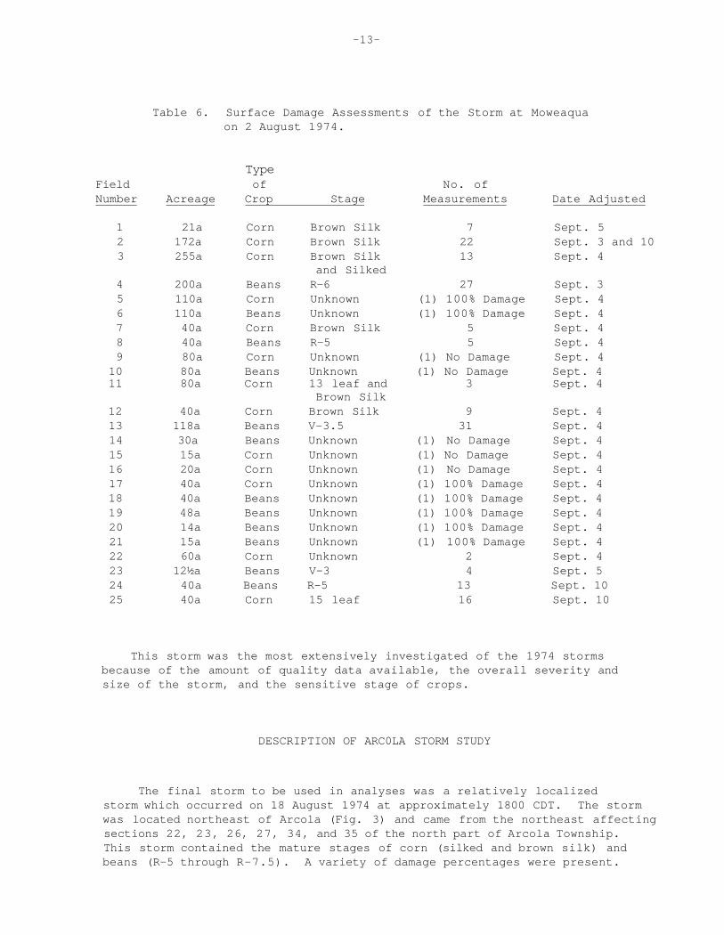
Table 6. Surface Damage Assessments of the Storm at Moweaqua on 2 August 1974.

Type Field of No. of Number Acreage Crop Stage Measurements Date Adjusted

1 21a Corn Brown Silk 7 Sept. 5 2 172a Corn Brown Silk 22 Sept. 3 and 10 3 255a Corn Brown Silk 13 Sept. 4

and Silked 4 200a Beans R-6 27 Sept. 3 5 110a Corn Unknown (1) 100% Damage Sept. 4 6 110a Beans Unknown (1) 100% Damage Sept. 4 7 40a Corn Brown Silk 5 Sept. 4 8 40a Beans R-5 5 Sept. 4 9 80a Corn Unknown (1) No Damage Sept. 4

10 80a Beans Unknown (1) No Damage Sept. 4 11 80a Corn 13 leaf and 3 Sept. 4

Brown Silk 12 40a Corn Brown Silk 9 Sept. 4 13 118a Beans V-3.5 31 Sept. 4 14 30a Beans Unknown (1) No Damage Sept. 4 15 15a Corn Unknown (1) No Damage Sept. 4 16 20a Corn Unknown (1) No Damage Sept. 4 17 40a Corn Unknown (1) 100% Damage Sept. 4 18 40a Beans Unknown (1) 100% Damage Sept. 4 19 48a Beans Unknown (1) 100% Damage Sept. 4 20 14a Beans Unknown (1) 100% Damage Sept. 4 21 15a Beans Unknown (1) 100% Damage Sept. 4 22 60a Corn Unknown 2 Sept. 4 23 12½a Beans V-3 4 Sept. 5 24 40a Beans R-5 13 Sept. 10 25 40a Corn 15 leaf 16 Sept. 10

This storm was the most extensively investigated of the 1974 storms because of the amount of quality data available, the overall severity and size of the storm, and the sensitive stage of crops.

DESCRIPTION OF ARC0LA STORM STUDY

The final storm to be used in analyses was a relatively localized storm which occurred on 18 August 1974 at approximately 1800 CDT. The storm was located northeast of Arcola (Fig. 3) and came from the northeast affecting sections 22, 23, 26, 27, 34, and 35 of the north part of Arcola Township. This storm contained the mature stages of corn (silked and brown silk) and beans (R-5 through R-7.5). A variety of damage percentages were present.

Table 7. Surface Data Points by Crop Stage and Percent Damage (By 10 Percent Intervals).

MOWEAQUA

Percent Damage Stage 0-10 10 -20 20 -30 30 -40 40-50 50-60 60 -70 70 -80 80 -90 90 -100

Sub Total Total

13 leaf 15 leaf Brown Silk

0 0 19

0 0 9

1 2 3

0 2 4

1 2 4

0 3 0

0 0 3

0 1 4

0 3 4

1 3 13

3 16 63

Subtotal 19 9 6 6 7 3 3 5 7 17 82

V-3 V-3.5 R-5 R-6

2 0 2 0

0 3 3 1

1 3 2 2

0 1 3 2

1 3 3 5

0 5 2 3

0 4 1 1

0 3 2 3

0 3 1 4

0 6 1 11

4 31 20 32

Subtotal 4 7 8 6 12 10 6 8 8 18 87

-15-

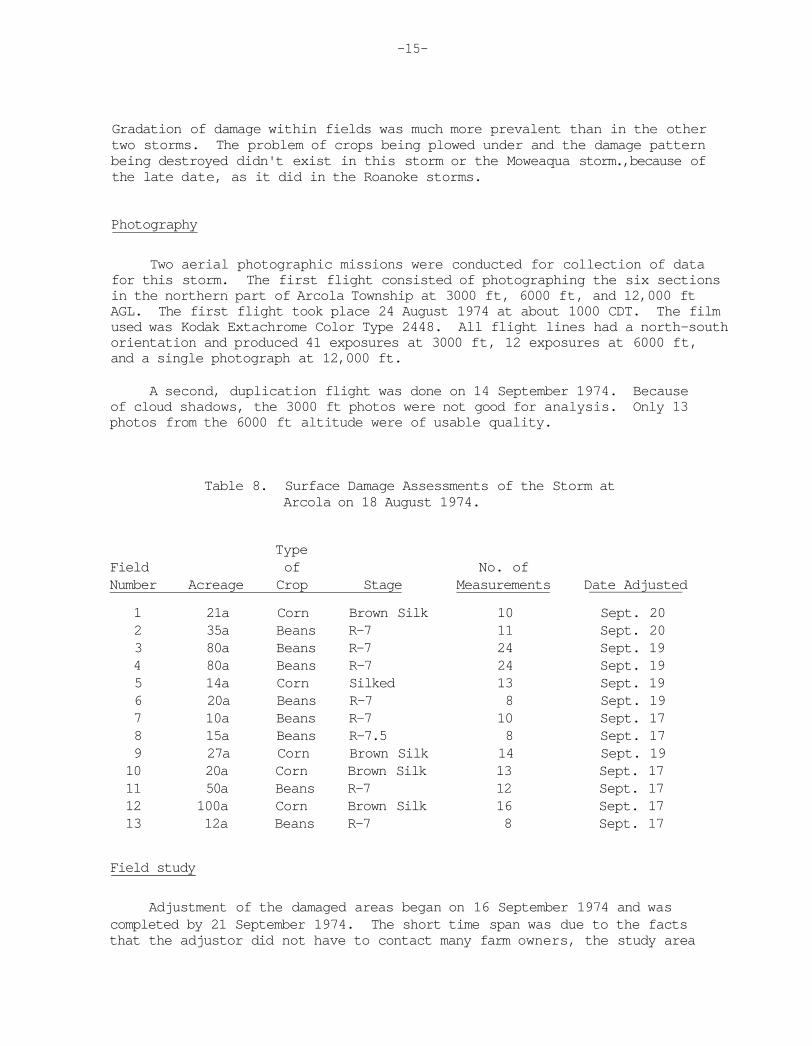
Gradation of damage within fields was much more prevalent than in the other two storms. The problem of crops being plowed under and the damage pattern being destroyed didn't exist in this storm or the Moweaqua storm.,because of the late date, as it did in the Roanoke storms.

Photography

Two aerial photographic missions were conducted for collection of data for this storm. The first flight consisted of photographing the six sections in the northern part of Arcola Township at 3000 ft, 6000 ft, and 12,000 ft AGL. The first flight took place 24 August 1974 at about 1000 CDT. The film used was Kodak Extachrome Color Type 2448. All flight lines had a north-south orientation and produced 41 exposures at 3000 ft, 12 exposures at 6000 ft, and a single photograph at 12,000 ft.

A second, duplication flight was done on 14 September 1974. Because of cloud shadows, the 3000 ft photos were not good for analysis. Only 13 photos from the 6000 ft altitude were of usable quality.

Table 8. Surface Damage Assessments of the Storm at Arcola on 18 August 1974.

Type Field of No. of Number Acreage Crop Stage Measurements Date Adjusted

1 21a Corn Brown Silk 10 Sept. 20 2 35a Beans R-7 11 Sept. 20 3 80a Beans R-7 24 Sept. 19 4 80a Beans R-7 24 Sept. 19 5 14a Corn Silked 13 Sept. 19 6 20a Beans R-7 8 Sept. 19 7 10a Beans R-7 10 Sept. 17 8 15a Beans R-7.5 8 Sept. 17 9 27a Corn Brown Silk 14 Sept. 19 10 20a Corn Brown Silk 13 Sept. 17 11 50a Beans R-7 12 Sept. 17 12 100a Corn Brown Silk 16 Sept. 17 13 12a Beans R-7 8 Sept. 17

Field study

Adjustment of the damaged areas began on 16 September 1974 and was completed by 21 September 1974. The short time span was due to the facts that the adjustor did not have to contact many farm owners, the study area

-16-

Figure 3. Area Photographed for Arcola Storm.

Table 9. Surface Data Points by Crop Stage and Percent Damage (By 10 Percent Intervals).

ARCOLA

Percent Damage Stage 0-10 10-20 20-30 30 -40 40--50 50 -60 60-70 70 -80 80-90 90--100

Sub Total Total

Silked Brown Silk

0 6

0 14

0 6

0 6

1 5

1 2

10 5

0 5

0 2

0 0 12

51 Subtotal 6 14 6 6 6 3 15 5 2 0 63

R-7 R-7.5

8 3

7 2

7 3

8 0

9 0

5 0

10 0

6 0

10 0

23 0

93 8

Subtotal 11 9 10 8 9 5 10 6 10 23 101

-18-

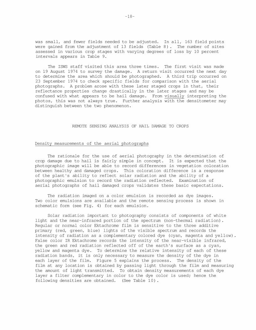
was small, and fewer fields needed to be adjusted. In all, 163 field points were gained from the adjustment of 13 fields (Table 8). The number of sites assessed in various crop stages with varying degrees of loss by 10 percent intervals appears in Table 9.

The ISWS staff visited this area three times. The first visit was made on 19 August 1974 to survey the damage. A return visit occurred the next day to determine the area which should be photographed. A third trip occurred on 23 September 1974 to check specific fields for comparison with the aerial photographs. A problem arose with these later staged crops in that, their reflectance properties change drastically in the later stages and may be confused with what appears to be hail damage. From visually interpreting the photos, this was not always true. Further analysis with the densitometer may distinguish between the two phenomenon.

REMOTE SENSING ANALYSIS OF HAIL DAMAGE TO CROPS

Density measurements of the aerial photographs

The rationale for the use of aerial photography in the determination of crop damage due to hail is fairly simple in concept. It is expected that the photographic image will be able to record differences in vegetation coloration between healthy and damaged crops. This coloration difference is a response of the plant's ability to reflect solar radiation and the ability of a photographic emulsion to record the radiation reflected. Examination of aerial photographs of hail damaged crops validates these basic expectations.

The radiation imaged on a color emulsion is recorded as dye images. Two color emulsions are available and the remote sensing process is shown in schematic form (see Fig. 4) for each emulsion.

Solar radiation important to photography consists of components of white light and the near-infrared portion of the spectrum (non-thermal radiation). Regular or normal color Ektachrome film is sensitive to the three additive primary (red, green, blue) lights of the visible spectrum and records the intensity of radiation as a complementary colored dye (cyan, magenta and yellow). False color IR Ektachrome records the intensity of the near-visible infrared, the green and red radiation reflected off of the earth's surface as a cyan, yellow and magenta dye. To determine the relative intensity of each of these radiation bands, it is only necessary to measure the density of the dye in each layer of the film. Figure 5 explains the process. The density of the film at any location is obtained by passing light through the film and measuring the amount of light transmitted. To obtain density measurements of each dye layer a filter complementary in color to the dye color is used; hence the following densities are obtained. (See Table 10).

-19-

Figure 4.

Figure 5.

-20-

Table 10. Density Measurements from Normal and False Color Films.

Regular Color False Color Film In Film

Color Filter R G B R G B on Densitometer Dye Layer C M Y C M Y Corresponding Band of R G B IR R G Reflected Radiation

The actual density value is calculated as follows;

Opacity is defined as the ratio of light incident on a film to the light transmitted or Opacity = Density is defined as the logarithm of opacity or Density = Log

Table 11 illustrates these measures.

Table 11. Opacity, Density Measures.

% Light Opacity Density Transmitted Li/Lt Log (Li/Lt)

100 100/100 = 1 0 10 100/ 10 = 10 1 1 100/ 1 = 100 2 0.1 100/ 0.1 = 1,000 3 0.01 100/ 0.01 = 10,000 4

These measures are then used to quantify the radiation reflected off a ground target as recorded on film. Unfortunately, although damage to crops alters their reflecting properties, other variables are involved. Atmospheric conditions, crop stage, scale of photography, differences in emulsions and processing, background soil color, densitometer characteristics and calibration and time of flight after storm all affect the record of the radiation response of the film. To determine the relationship between crop damage and density measurements, statistical processing is necessary.

-21-

Statistical modeling

The first part of the modeling procedure to be developed for the project was to simply record the density readings from the photography. This was done for each field, within the flight line, in which an adjuster had made an evaluation of the damage and indicated the location points of his sampling. The data were then subjected to a data screening program which does the following:

1. Lists the data for each field according to crop type for a single flight line. Identification information includes a field number, a photograph number, the altitude of the photograph, date and time it was taken, crop type and stage, and the number of data points measured. Data includes a point identification density readings for the red, green, blue and visual transmissions and percent damage assessed (Table 12).

2. Plots scatter diagrams for the percent damage vs. each band (R, G, B) of raw density value.

3. Calculates the simple linear correlation coefficient for the regression line of the scatter diagram of raw densities vs. percent damage.

4. Ratios two bands of the raw densities and plots them against the percent damage.

5. Calculates the simple linear correlation coefficient for the regression line of the scatter diagram of the ratio of raw densities vs. percent damage. (See Fig. 6).

The above steps (2-5) are then repeated for all of the field data amalgamated as one data set.

This data screening has proved to be an invaluable aid in obtaining a first look at the information and the trends in the relationship between crop damage and densities. Two important results were obtained from this modeling; 1. The ratioing technique improves the correspondence between density vs. percent crop damage, 2. The greatest scatter occurs at either extreme of the percent damage (0% or 100% damage).

The first result was expected as ratioing density values has a tendency to remove some of the noise (atmospheric conditions, normal differences in coloration, angle of incidence of the Sun, etc.) from the raw measurements. The second result was not anticipated and predictions of crop damage at either extreme (near 0% or 100%) becomes unreliable.

An alternative approach to modeling the relationship between crop damage and density was attempted using multiple-curvilinear regression techniques. A three dimensional regression model was fitted to the data of the form;

-22-

Table 12. Computer Output of Surface and Spectral Data for Assessment Points of Damaged Corn Fields at Roanoke.

Figure 6. Scatter Diagram of Ratioed Spectral Data for a Damaged Corn Field in the Roanoke Storm.

-24-

Equation 1

W = a0 + a1X + a2Y + a3Z

where W = percent crop damage X = B density value Y = G density value Z = R density value

X, Y, and Z are density values recorded on the densitometer -depending on which film is being used. Their values correspond to different radiation bands. (See Table 10).

This equation can be expanded by increasing the powers (degree) of the terms to include more complex envelopes fitting the data. The improvement in prediction ability is rewarding and the investigation will pursue the refinement of this model for use as the prediction method. Table 13 presents computer printout of the prediction model for the damaged corn fields in Roanoke. In the Table x-value is the red/green ratioed density value, y-value is the green/blue ratioed density value, z-value is the actual loss assessment, z-predicted is the predicted loss from the model, and the residual is the difference in the actual and predicted assessments.

The coefficient of correlation of 0.927 is very high (a perfect correlation is 1.00). It means that 86% (the square of 0.927) of the loss variability is explained by the technique.

It is apparent then that the use of this model involves a priori knowledge of crop damage on the ground. Because of the variations within the system, it is impossible to develop a table of densities vs. crop damage, and each flight taken at different times will have to be calibrated. This involves sampling a small number of fields on the ground to estimate crop damage, recording of the densities for the same fields from the film and then using the computer to develop the model as shown in Equation 1. The amount of crop damage to the remaining fields, recorded on the same flight, can be predicted by measuring the densities of the fields on the photography and entering them in Equation 1. The results of this modeling can then be displayed as a computer derived map in which the percent damage is shown as contoured display. The map scale can be accurately determined and the area corresponding to each class of percent damage calculated.

A simplified version of this program is now completed and the results of a trial run are shown in Fig. 7. The statistics with the map indicate the area of each class of percent damage and frequency of that damage class for the field. Additional calculations could easily be added to the existing algorithm. For instance, claim figures could be entered and using the statistics generated from the map and a final adjustment figure could be computed.

-25-

Table 13. Computer Output of Prediction Model for the Damaged Corn Fields at Roanoke.

-26-

Figure 7. Map and Areal Statistics of a Damaged Corn Field at Roanoke Reconstructed from the Aerial Photography and Computer Model.

-27-

The system design

Much of the work completed has been tailored to the establishment of a simple workable system with which an individual would be able to estimate crop damage and determine the statistics necessary to settle claims from photography and a minimal amount of ground truth sampling. The system as envisioned now would consist of the following steps:

1. After a storm, direct a flight be made of the area for acquisition of aerial photographs.

2. Initiate a ground truth operation of a sample of the fields within the overflight area.

3. Determine what fields on the imagery correspond to the sampled fields and take density readings at the spot locations where the adjuster has estimated percent damage.

4. Insert these data into the multiple regression program and obtain estimates (coefficients) of the model for prediction of loss.

5. Systematically sample the remaining fields in the flight line obtaining 20-30 density readings per field with the densitometer. Using the estimates (coefficients) of the multiple-curvilinear model and the systematically sampled data, enter all of it into the mapping program.

6. Results for all fields will be printed maps showing percent damage statistics and patterns similar to Fig. 7.

Although this system is currently operational, it contains only very basic capabilities. Much work needs to be done to refine the modeling procedures, and a validity check of the refined system will eventually be necessary. Much of the future investigation, as far as the remote sensing data analysis techniques are concerned, will be centered around the following items:

1. An examination and modeling of the crop stages as a variable affecting the differences in the density values recorded on the film.

2. An examination and modeling of the effect of photographic scale and lag time of the photography after the storm on the density values recorded on the film.

3. Comparison of the discrimination ability of normal color film vs. the color infrared film.

4. Analysis of density values obtained by scanning an entire photograph.

-28-

5. Possible use of an alternate envelop modeling technique which fits the data exactly rather than statistically (least squares) as currently being used.

6. Development of a spatial sampling (coordinate locations) system for the systemmatic sampling of densities in the unknown fields in the flight line.

7. Determining the optimal ground truth sample size for 95% or better prediction capability.

8. Development of a method to remove water damaged areas from the area statistics.

9. Include means of determining crop damage estimates from early (young crop stage) in the season photography.

10. Develop a system through which the results of a previous year's work can be validated and used to improve the prediction model for the succeeding new season.

All of the above deals directly with the modeling programs used for prediction. Further examination of the adjuster's ability to estimate percent damage and area should be considered as well. Although his values are used for the calibration of the modeling system, it may be appropriate to examine and test his field method and recommend procedural changes which will aid in the development of a more accurately calibrated system. The reliability of the system is wholly dependent on an adjuster's ability to accurately sample a small set of fields within a flight. The system developed here will extend this subset of information to all fields within the flight line. The accuracy of the measurements and the estimates of the crop damage for these fields will be no better than the estimates for the subset sampled by the adjuster.

SUMMARY

The primary objective of this project was to determine the feasibility of aerial photography in assessing crop damage from hail. The 1974 photographic flights, surface loss assessments, and analysis discussed above demonstrated that a relationship between actual crop damage and that determined remotely by photographic analysis could possibly be established.

Further study needs to be done to refine the analysis techniques. More photographic and surface loss data are needed to obtain a statistically significant sample. Use of the advanced computer analysis techniques which were not available several years ago, indicate that false color infrared film needs to be re-investigated, particularly in the early crop stages. For instance, it might be better able to detect the damage (loss in quality and yield) after crops have recovered to some degree. Also, more research needs

-29-

to be done to determine the most efficient flight altitude. Increasing the altitude by 1500 ft, from 3000 to 4500 ft above ground level, will reduce the number of photographs by one-half.

The 1974 investigations revealed that photos from various altitudes (3000 to 12,000 ft) could be used to delineate major areas of damage. This gives strong indication that aerial photography can be used as an aid in planning and conducting storm surveys. It also gives indications that a relationship exist between crop damage and what is recorded on an aerial photograph.

Assuming that no major problems occur and sufficient data are collected in the second year (1975), we would hope to have the loss assessments technology developed by May 1976. The summer of 1976 should be viewed as a "test" and demonstrating period for the technology. This test would include aerial photography, surface calibration points, computer processing of these data, and resulting loss of yield determinations for selected fields.

ACKNOWLEDGMENTS

This project is deeply indebted to John R. Williams who conducted all the surface loss measurements, surveyed many storms, and offered many helpful suggestions. Thanks also goes to the many Country Companies Agencies and crop adjusters who notified us of potentially useful hailstorms.

REFERENCES

Barron, N. A., S. A. Changnon, Jr., and J. Hornaday, 1970: Investigations of crop-hail loss measurement techniques. Res. Rept. 42, Crop-Hail Insurance Actuarial Association, Chicago, 65 pp.

Changnon, S. A., Jr., and N. A. Barron, 1971: Quantification of crop-hail losses by aerial photography, J. Appl. Meteoro. , 10, 86-96.

Jackson, H. R., 1970: Corn aphid infestation computer analyzed from aerial color infrared, Photogrammetric Engineering, 40, 943-952.

Philpott, L. E., and V. R. Wallen, 1969: IR color for crop disease identification. Photogrammetric Engineering, 35, 1116-1125.