Remote Sensing of Environment 196 (2017) 193–204

Contents lists available at ScienceDirect

Remote Sensing of Environment

j ourna l homepage: www.e lsev ie r .com/ locate / rse

Enhanced forest cover mapping using spectral unmixing andobject-based classification of multi-temporal Landsat imagery

David Gudex-Cross ⁎, Jennifer Pontius, Alison AdamsThe Rubenstein School of Environment and Natural Resources, University of Vermont – Aiken Center, 81 Carrigan Drive, Burlington, VT 05405, United States

⁎ Corresponding author.E-mail address: dgudexcr@uvm.edu (D. Gudex-Cross)

http://dx.doi.org/10.1016/j.rse.2017.05.0060034-4257/© 2017 Elsevier Inc. All rights reserved.

a b s t r a c t

a r t i c l e i n f o

Article history:Received 7 November 2016Received in revised form 24 April 2017Accepted 8 May 2017Available online xxxx

Spatially-explicit tree species distribution maps are increasingly valuable to forest managers and researchers inlight of the effects of climate change and invasive pests on forest resources. Traditional forest classifications arelimited to broad classes of forest types with variable accuracy. Advanced remote sensing techniques, such asspectral unmixing and object-based image analysis, offer novel forest mapping approaches by quantifying pro-portional species composition at the pixel level and utilizing ancillary environmental data for forest classifica-tions. This is particularly useful in the Northeastern region of the United States where species composition isoften mixed.Here we employed a hierarchical forest mapping approach using spectral unmixing of multi-temporal Landsatimagery to quantify percent basal area for ten common tree species/genera across northern New York and Ver-mont. Basal areamapswere then refinedusing an object-based ruleset to produce a thematic forest classification.Validationwith 50 field inventory plots covering a range of species compositions indicated that the quality of per-cent basal areamapping largely reflected the number of “pure” (N80% BA) endmember plots available for calibra-tion, with more common species mapped at a higher accuracy (i.e. Acer saccharum, adj. r2 = 0.44, compared toPopulus sp., adj. r2 = 0.24). The resulting thematic forest classification mapped 15 forest classes (nine species/genus level and six common species assemblages) with overall accuracy = 42%, KHAT = 33%, fuzzy accuracy= 86% at the pixel level, and 38%, KHAT = 29%, fuzzy accuracy = 84% at the object level.Using the validation plots to compare existing forest classification products, this hierarchical approach providedmore class detail (11 represented classes) and higher accuracy than the National Forest TypeMap (six represent-ed classes, overall accuracy 18%, fuzzy accuracy 70%), LANDFIRE (five represented classes, overall accuracy 28%,fuzzy accuracy 80%) and National Land Cover Database (three represented classes, overall accuracy = 56%).These results show thatmore detailed and accurate forestmapping is possible using a combination ofmulti-tem-poral imagery, spectral unmixing, and rule-based classification techniques. Improved large-scale forest mappinghas important implications for natural resource management and other modeling applications.

© 2017 Elsevier Inc. All rights reserved.

Keywords:Remote sensingBasal area mappingBiophysical modelingHierarchical classificationObject-based image analysis

1. Introduction

Developing cost-effectivemethods to accurately classify forest coveris essential to inform sustainable forest management at local, regional,and national levels. These products are increasingly valuable in light ofthe anticipated effects of climate change and invasive pests on forest re-sources.Warming temperatures and changing precipitation regimes areexpected to cause shifts in tree species distributions (Hamann andWang, 2006; Iverson and Prasad, 2001; Tang et al., 2012) and increasesin the duration and severity of pest/pathogen outbreaks (Dale et al.,2001; Dukes et al., 2009). Yet our ability to direct management actionsis limited by the coarse detail and relatively low accuracy of existinglarge-scale forest cover maps.

.

Existing forest cover maps include field inventory and remote sens-ing based products, including those generated through the Forest Inven-tory and Analysis program (FIA; http://www.fia.fs.fed.us/), the NationalLand Cover Database (NLCD; http://www.mrlc.gov/) and LANDFIREExisting Vegetation Type (LANDFIRE EVT; http://www.landfire.gov/).More recently, the United States Forest Service (USFS) has also usedFIA data, multi-temporal Moderate Resolution Spectroradiometer(MODIS) imagery, vegetation indices, and other ancillary environmen-tal data to produce the National Forest Type map (National ForestType Map, http://data.fs.usda.gov/geodata/rastergateway/forest_type/index.php). The LANDFIRE and NLCD programs provide national foresttype maps at a 30 m × 30 m spatial resolution, but in coarser foresttype classes than FIA/USFS species-level products.

Several remote sensing studies have successfully mapped species-level distributions, though largely at highly localized spatial scales(Carleer and Wolff, 2004; Immitzer et al., 2012; Ke et al., 2010; Martin

194 D. Gudex-Cross et al. / Remote Sensing of Environment 196 (2017) 193–204

et al., 1998; Plourde et al., 2007). These studies typically rely on data-in-tensive hyperspectral and/or high spatial resolution imagery (e.g.Ikonos, QuickBird, WorldView-2, Airborne Visible/Infrared ImagingSpectrometer – AVIRIS, Light Detection and Ranging – LiDAR), limitingtheir applicability to tree species/genus classification across largerregions.

Wolter et al. (1995), Mickelson et al. (1998), and Hill et al. (2010)achieved relatively accurate species-type classifications by utilizingmulti-temporal Landsat imagery, demonstrating the usefulness of ac-quiring multiple image dates that capture phenologically-significantdifferences among species (e.g. green-up, senescence, etc.). Dymondet al. (2002) also found improved deciduous forest type discriminationwhen multi-temporal Landsat imagery was supplemented with Nor-malized Difference Vegetation Index (NDVI) and Tasseled Cap Transfor-mation (TC) bands, as well as their respective differences among imagedates.

Advanced remote sensing techniques, such as spectral unmixing andobject-based image analysis (OBIA), utilize a wealth of spectral, spatial,and ancillary environmental data to enable more precise forest covermapping (see Pu, 2013 for reviews; Xie et al., 2008). Spectral unmixinghas been shown to outperform traditional pixel-based classifiers bydecomposing (“unmixing”)mixed pixels and assigning component pro-portions at the subpixel level (Huguenin et al., 1997; Oki et al., 2002).This is particularly useful in northeastern forests where species com-position is often heterogeneous. The resulting per-pixel proportionsof each species obtained from the spectral unmixing process alsofacilitate the mapping of other forest attributes that are dependentupon the complexity of species composition common in northeast-ern forests (e.g. carbon storage, basal area, productivity) (Hall etal., 1995; Sonnentag et al., 2007; Yan et al., 2015). OBIA techniquesovercome individual pixel constraints by segmenting imagery intohomogenous “objects” upon which classification is then carriedout. This allows for the additional characterization of shape, size,and texture into classifications and minimizes impacts of canopyarchitecture-driven variability in spectral signatures (Chubey et al.,2006).

While OBIA is often more accurate than pixel-based methods formapping forest cover at high spatial resolutions (Agarwal et al., 2013;Dorren et al., 2003; Oruc et al., 2004), comparative studies indicatethat coupling pixel-based and OBIA techniques can improve the accura-cy of forest type classifications (Aguirre-Gutiérrez et al., 2012; Wang etal., 2004). Using Ikonos imagery, Wang et al. (2004) achieved thehighest mangrove classification accuracies when integrating a pixel-level classification to identify spectrally-distinct classes, then carryingout an object-based nearest neighbor analysis on spectrally-mixed clas-ses. Similarly, Aguirre-Gutiérrez et al. (2012) obtained the highest accu-racy in montane landscapes when merging the best pixel-based andobject-based classes to produce the final thematic land coverclassification.

Here, we test a novel approach to tree species mapping that inte-gratesmanyof the successful approaches used in these previous studies.This involves pixel-level spectral unmixing that integratesmulti-tem-poral Landsat imagery to develop percent basal area coverages for 10common species. These percent basal area coverages are then incorpo-rated into an object-based hierarchical ruleset to generate 16 forestclasses (10 species/genera and 6 common assemblages). To evaluatethe utility of this integrated multi-temporal, spectral unmixing(MTSU) approach,we compare accuracywith existing large-scale forestmapping products, including LANDFIRE EVT, National Forest Type Map,and NLCD.

Achieving accurate, species-specific forest classifications isnecessary to fill critical gaps in our knowledge of current tree speciesdistributions. This integrated approach attempts to maximize the ac-curacy and detail possible from widely available Landsat imagery,allowing for improved, widespread mapping of important forestresources.

2. Methods

2.1. Study area and base imagery

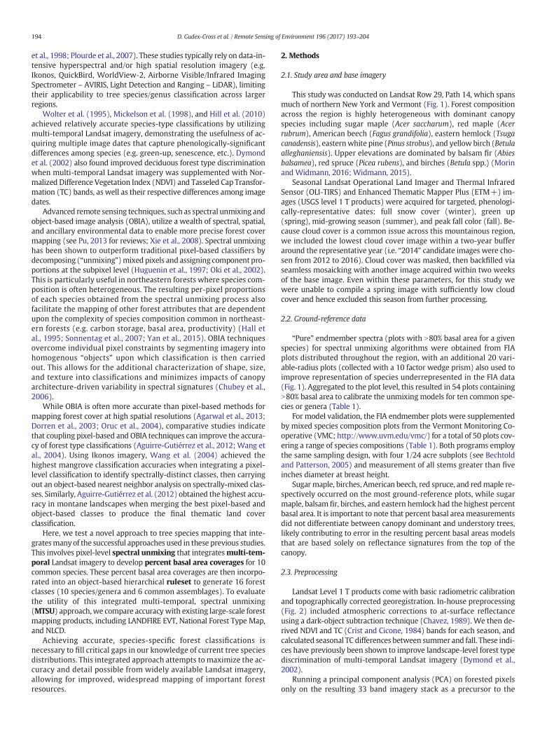
This study was conducted on Landsat Row 29, Path 14, which spansmuch of northern New York and Vermont (Fig. 1). Forest compositionacross the region is highly heterogeneous with dominant canopyspecies including sugar maple (Acer saccharum), red maple (Acerrubrum), American beech (Fagus grandifolia), eastern hemlock (Tsugacanadensis), easternwhite pine (Pinus strobus), and yellow birch (Betulaalleghaniensis). Upper elevations are dominated by balsam fir (Abiesbalsamea), red spruce (Picea rubens), and birches (Betula spp.) (Morinand Widmann, 2016; Widmann, 2015).

Seasonal Landsat Operational Land Imager and Thermal InfraredSensor (OLI-TIRS) and Enhanced Thematic Mapper Plus (ETM+) im-ages (USGS level 1 T products) were acquired for targeted, phenologi-cally-representative dates: full snow cover (winter), green up(spring), mid-growing season (summer), and peak fall color (fall). Be-cause cloud cover is a common issue across this mountainous region,we included the lowest cloud cover image within a two-year bufferaround the representative year (i.e. “2014” candidate images were cho-sen from 2012 to 2016). Cloud cover was masked, then backfilled viaseamless mosaicking with another image acquired within two weeksof the base image. Even within these parameters, for this study wewere unable to compile a spring image with sufficiently low cloudcover and hence excluded this season from further processing.

2.2. Ground-reference data

“Pure” endmember spectra (plots with N80% basal area for a givenspecies) for spectral unmixing algorithms were obtained from FIAplots distributed throughout the region, with an additional 20 vari-able-radius plots (collected with a 10 factor wedge prism) also used toimprove representation of species underrepresented in the FIA data(Fig. 1). Aggregated to the plot level, this resulted in 54 plots containingN80% basal area to calibrate the unmixing models for ten common spe-cies or genera (Table 1).

For model validation, the FIA endmember plots were supplementedby mixed species composition plots from the Vermont Monitoring Co-operative (VMC; http://www.uvm.edu/vmc/) for a total of 50 plots cov-ering a range of species compositions (Table 1). Both programs employthe same sampling design, with four 1/24 acre subplots (see Bechtoldand Patterson, 2005) and measurement of all stems greater than fiveinches diameter at breast height.

Sugarmaple, birches, American beech, red spruce, and redmaple re-spectively occurred on the most ground-reference plots, while sugarmaple, balsam fir, birches, and eastern hemlock had the highest percentbasal area. It is important to note that percent basal area measurementsdid not differentiate between canopy dominant and understory trees,likely contributing to error in the resulting percent basal areas modelsthat are based solely on reflectance signatures from the top of thecanopy.

2.3. Preprocessing

Landsat Level 1 T products come with basic radiometric calibrationand topographically corrected georegistration. In-house preprocessing(Fig. 2) included atmospheric corrections to at-surface reflectanceusing a dark-object subtraction technique (Chavez, 1989). We then de-rived NDVI and TC (Crist and Cicone, 1984) bands for each season, andcalculated seasonal TC differences between summer and fall. These indi-ces have previously been shown to improve landscape-level forest typediscrimination of multi-temporal Landsat imagery (Dymond et al.,2002).

Running a principal component analysis (PCA) on forested pixelsonly on the resulting 33 band imagery stack as a precursor to the

Fig. 1. The study area, spanning northern New York and Vermont, and distribution of ground-reference plots (Landsat Path 14, Row 29).

195D. Gudex-Cross et al. / Remote Sensing of Environment 196 (2017) 193–204

Minimum Noise Fraction (MNF) transform (see Section 2.4 below)allowed us to minimize autocorrelation among the full component ofinput bands. This step removed noise inherent in many of these bandsdue to differences in illumination and atmospheric conditions acrossdifferent image acquisition dates, and isolated the spectral signal specif-ic to distinguishing forested pixels.

The final stacked image for spectral unmixing included the firstthree PCA bands (accounting for N99% of the spectral variability in thefull 33-band stack). Because these PCA bands were primarilydistinguishing among species composition (see Section 3.1), the finalstacked image also included summer Landsat reflectance bands, NDVI,Tasseled Cap, and Tasseled Cap difference vegetation index products(Fig. 2) to capture information about canopy density for percent basalarea modeling.

Table 1The species composition of ground-reference plots used for development of percent basalarea (%BA) models.

Tree spp./genus No. of pureendmember plots

Mean %BA(±SD)

Max %BA No. of plotsw/species

Balsam fir 8 14.3 (27.7) 92.5 14Red maple 2 6.7 (14.2) 80.5 18Sugar maple 10 27.7 (36.6) 96.0 27Birches 6 13.1 (20.4) 80.7 26American beech 2 6.3 (13.2) 81.8 22Red spruce 1 5.7 (14.6) 92.0 20Eastern white pine 11 5.8 (21.4) 100.0 6Aspens 1 3.3 (13.8) 86.5 5Oaks 2 3.4 (13.1) 65.0 4Eastern hemlock 11 9.2 (25.0) 93.1 10

2.4. Spectral unmixing

The spectral unmixing process outlined here largely follows that de-veloped by Nielsen (2001) and Boardman and Kruse (2011), which haspreviously been used to classify tree specieswith hyperspectral imagery(see Hallett et al., 2010; Plourde et al., 2007). AMNF transformwas firstapplied to the final imagery stack (17 bands) for data decorrelation andspectral noise reduction (Green et al., 1988) (Fig. 2). Endmember pixelswere refined using a Pixel Purity Index to ensure spectral similarity ofMNF bands among geographically distinct sites, with spectral outliersbeing excluded from further analysis. The resulting MNF image wasthen “unmixed” using aMixture-tunedMatched Filtering (MTMF) algo-rithm (Boardman, 1998) based on the target endmember spectra (i.e.tree species signatures). MTMF is a form of spectral mixture analysisthat employs partial linear unmixing to map the abundance or fractionof target endmember spectra within each pixel (Boardman and Kruse,2011). The MTMF output consists of a matched filter and infeasibilityscore for each pixel, with the former reflecting how well the pixelmatches the target spectra and the latter representing the likelihoodof a false positive.

We considered several approaches to model percent basal area forinput into the object-based classification ruleset based on the MTMFproducts. The traditional approach involves identifying thresholds formatched filter and infeasibility scores to maximize the binary accuracyof a species' presence/absence. Because we were mapping heteroge-neous forest cover dominated by mixed species composition, such a bi-nary classification was ruled out for our purposes. Regression modelshave also been used to map species fractional basal area usinghyperspectral imagery (Pontius et al., 2005). This study differed from

Fig. 2. The Landsat preprocessing and percent basal area modeling workflow.

196 D. Gudex-Cross et al. / Remote Sensing of Environment 196 (2017) 193–204

these previous single species efforts based on the large number ofground-reference plots across a range of forest species composition.The diverse plot network resulted in a variable number of plots wherethe target species was completely absent, as well as a suite of possiblematched filter and infeasibility scores derived from the 10 speciesunmixing products.

Using linear regression models based only on plots that containedthe species of interest produced more stable regression metrics, but re-sulted inmany false positives where particular species were absent. Wealso tested zero-inflated regression to account for the propensity of zerobasal area plots in the calibration data. Results were generally lowermodel fit than the general linear models, with continued over-predic-tion of zero basal area plots. Further, zero-inflation p-values resultingfrom regression estimates were not significant, indicating that the pres-ence of zero value data was not a significant contributor to overallmodel variability.

Our most consistently accurate results came from a stepwise linearregression model that included all ground-reference plots (includingthose where the target species was absent). Model terms were limitedto match filter and infeasibility variables significant at the 0.05 level,with amaximum variance inflation factor of 10 to avoid autocorrelationamong parameters. We used the minimum Bayesian Information Crite-rion (Bhat and Kumar, 2010) to select the best fit model. The resultingregression equation was then applied to the MTMF image via bandmath to create a percent basal area raster for each target species/genus.

It is important to note that the resulting fractional basal area prod-ucts were not intended to be stand-alone products, but instead to beused as inputs to quantify the relative abundance of species withineach pixel in order to inform classification. These relative abundanceswere not aggregated for all species but instead used as independent in-puts to the object-based hierarchical ruleset (see Section 2.5 below).

2.5. Object-based classification

Percent basal area rasters obtained from the pixel-based spectralunmixing were then incorporated into an object-based, hierarchicalruleset classification scheme (Fig. 3). This allowed us to refine the per-cent basal area products using ancillary environmental data (i.e. digitalelevation data from theNational ElevationDataset available through theU.S. Geological Survey) and produce classifications on a stand- versuspixel-level.

Object-based classifications begin with segmentation to aggregatelike pixels into larger image objects. Segmentation settings and inputlayer weightings were informed by knowledge of the image resolution,spatial characteristics of the landscape, and spectral nature of the fea-ture objects. As is common in object-based classifications, iterations ofvarious settings were evaluated to confirm selection of final segmenta-tion settings. We used a multiresolution segmentation algorithm (seeChubey et al., 2006 for further explanation) based on layer inputs thathighlighted differences in vegetation characteristics across our studyarea. This included weighting the first three MNF bands most, followedby summer and winter NDVI and seasonal TC differences. Given themoderate spatial resolution of Landsat imagery and heterogeneous na-ture of forest composition patterns across the landscape, a very lowscale parameter (1) with no shape or compactness weighting wasused for object segmentation. To compare the pixel-level ruleset resultsto this object-based approach, a chessboard segmentation with a scaleparameter of 1 and no band weighting was used to create pixel“objects”.

The ruleset started by differentiating forest from non-forest objectsusing thresholds for winter band 3 leveraging snow cover (non-forestN 0.60), and spring band 4, masking water (non-forest b 0.065). Forestclasses were then assigned based on percent basal area rasters and

Fig. 3. The object-based image analysis (OBIA) workflow to generate a 16-class thematic forest cover map.

Table 2Principal components analysis eigenvectors highlight the input bands that account for themost spectral variability among forested pixels.

Input band PCA band Eigenvector

Fall band 5 (mid-IR) 1 0.233Fall band 2 (green) 1 0.207Fall band 4 (NIR) 2 0.295Fall NDVI 2 0.271

197D. Gudex-Cross et al. / Remote Sensing of Environment 196 (2017) 193–204

elevational constraints outlined by Burns and Honkala (1990) (Fig. 3)following a rule-based hierarchy. A species/genus class was assigned ifthe object contained N40% basal area of that species or genus and didnot exceed the specified elevation threshold (if there was one). Sincerare species are spottier across the landscape and more likely to besmoothed out when averaged within image objects, forest type assign-ment in the hierarchical ruleset progressed from the least to most com-mon species to maximize representation of rare species in the finalthematic classification.

To capture regionally-common species assemblages where no spe-cies was N40% basal area, we also classified six common forest assem-blages by summing the percent basal area values for their respectivecomponent species (Fig. 3). The final thematic forest classification of16 possible forest types was then exported as a 30-m by 30-m rasterproduct.

2.6. Accuracy assessment

Inventory data for the FIA and VMC plots described above (seeSection 2.2) were used to assign a forest class according to the samerule thresholds applied to the imagery. A confusionmatrix of actual ver-sus predicted forest classes was created to examine overall, kappa,User's, and Producer's accuracies. We also determined fuzzy accuracyby allowing misclassification between common species/species assem-blages. For example, we considered sugarmaple pixels that were classi-fied as northern hardwoods to be “correct” at the fuzzy level.

We similarly calculated accuracy for three existing forest mappingproducts: the 2011 LANDFIRE EVT classification; the National ForestType Map classification; and the 2011 NLCD classification. Only theLANDFIRE and National Forest Type Map classifications could be com-pared at the species-type level, with accuracy being determined follow-ing the same process outlined above with field plots assigned to matchtheir respective classes. For the NLCD product, we classified the valida-tion data as deciduous (N75% deciduous species), evergreen (N75% ev-ergreen species), or mixed forest (a plot was considered mixed whenboth deciduous and evergreen species were present but neitherexceeded 75% of the plot basal area).

3. Results and discussion

3.1. Spectral decomposition

Our approach included the aggregation of a variety of image datesand vegetation index products in order to maximize the spectral infor-mation available to differentiate physiologically similar species. Eigen-vectors from spectral decomposition were used to identify whichbands accounted for the most variability among forested pixels. Fromthe full 33 band multi-temporal stack, the largest eigenvectors camefrom the fall image (Table 2). It is important to keep in mind that thisPCA was run on forested pixels only in order to isolate the potentialspectral signal specific to differentiation among forest types (not for-est/non-forest). The fall image was timed at the peak of physiologicaldifferentiation among species for our region, providing key spectral in-formation to help separate otherwise spectrally similar species. Otherstudies have also cited the importance of using shoulder seasons withunique phenological information to assist in species classification(Dymond et al., 2002; Hill et al., 2010).

3.2. Percent basal area modeling

MTMF models of percent basal area resulted in significant but rela-tively weak (adj. r2 = 0.24; RMSE = 0.04, Populus sp.) to moderate re-lationships (adj. r2 = 0,59; RMSE = 0.06, American beech). Theserelatively low model fits likely result from several sources of knownerror. The sensor primarily records the spectral reflectance from the

198 D. Gudex-Cross et al. / Remote Sensing of Environment 196 (2017) 193–204

canopy surface, with a mix of canopy dominant trees that may differfrom understory composition included in ground-reference inventories.Further, percent basal area is based on main trunk diameter at breastheight with no accounting for variability in crown size or geometryamong species. This is reflected in lower fit statistics for species thatare more common in the understory of Northeastern forests (e.g. east-ern hemlock), or with relatively small crown geometry relative to com-mon co-occurring species.

The lack of fit is likely also driven by the preponderance of “pure”species plots included in the validation dataset. This resulted in plotswith extreme high and extreme low (zero occurrence) values of eachtarget species, levels where regression models are typically weakest.Species/genera with the lowest percent basal area fit were those withthe fewest endmember calibration plots and lowest general abundanceacross the study area (per FIA forest demographic reports). For thesetarget species, percent basal area was typically under-predicted (Table3). The most accurate percent basal area models were associated withthe dominant species in our region (e.g. American beech).

These results are similar other species mapping efforts. Savage et al.(2015) used a zero-inflated regressionmodel, based on a two-step pro-cess, to first predict the presence or absence of the target species andthen species composition only where the target species was present.They modeled five different conifer species in heterogeneous forests ofnorthwesternMontana using Landsat TMandOLI imagery, reporting in-dependent accuracy assessment RMSE from 0.11 to 0.23 (no r2 valueswere reported). These errors are slightly higher than the range ofRMSE values reported for our ten target species (0.04 to 0.16).

Moisen et al. (2006) compared generalized additive regressionmodeling, classification and regression tree (CART) techniques, and sto-chastic gradient boosting for modeling live basal area from multi-tem-poral Landsat imagery for thirteen tree species in Utah. Basal areaprediction results for all modeling techniques were poor for most spe-cies (r2 b 0.5 and RMS errors N 0.8). While the general approachemployed by Moisen et al. (2006) is similar to that described here(multi-temporal Landsat imagery), our range ofmodel fit is higher, indi-cating that the additional image processing techniques and spectralunmixing approach employed here may improve abundance mappingusing Landsat imagery.

Our percent basal area modeling results also compare favorably tothose obtained in other studies using MTMF techniques. Hyperspectralimagery, with its wealth of narrow reflectance bands, is well suited tospectral unmixing and species abundance mapping. Hyperspectral in-struments have reported comparable accuracy to that reported herefor eastern hemlock abundance in the Catskills region (r2 = 0.65;RMSE 0.12, Pontius et al. (2005)). Plourde et al. (2007) used spectralunmixing to model percent sugar maple and American beech in NewHampshire using both hyperspectral AVIRIS imagery as well as modifi-cations of the hyperspectral imagery to match broadband sensors. Theyfound weak relationships between field-measured and predicted per-cent basal area based on the broadband imagery, but results similar tothose reported here for spectral unmixing of the full hyperspectral

Table 3Percent basal area model fits derived from spectral unmixing.

Tree spp./genus r2 Adj. r2 Mean %BA RMSE PRESS RMSE

Balsam fir 0.34 0.32 0.15 0.11 0.12Red maple 0.47 0.46 0.08 0.06 0.06Sugar maple 0.46 0.44 0.28 0.16 0.17Birches (Betula spp.) 0.32 0.30 0.13 0.08 0.09American beech 0.60 0.59 0.07 0.06 0.07Red spruce 0.52 0.51 0.07 0.06 0.06Eastern white pine 0.3 0.29 0.1 0.1 0.1Aspens (Populus spp.) 0.25 0.24 0.04 0.04 0.04Oaks (Quercus spp.) 0.49 0.48 0.05 0.05 0.05Eastern hemlock 0.32 0.30 0.11 0.09 0.1

data (r2 = 0.49; RMSE = 0.09 for sugar maple and r2 = 0.36; RMSE= 0.18 for beech).

These studies collectively underscore that modeling continuous var-iables, like individual tree species basal area, is a difficult task. Clearlythe spatial resolution of Landsat imagery is limiting for mapping forestcover at the species level in highly mixed forests. Difficulties associatedwith scaling field data to the Landsat pixel level include: overlap in can-opy dominant species (Hallett et al., 2010; Plourde et al., 2007); incon-gruities between fieldmeasurements (which include understory stems)and sensor-derived canopy reflectance (particularly for shade-tolerantspecies such as hemlock); and incorrect registration between calibra-tion field plots and pixel centers. Atmospheric and topographic shadowimpacts on spectra are also particularly troublesome inmountainous re-gions. Within-species spectral variability due to differences in treehealth can also confound unmixing algorithms (Carter, 1993; Plourdeet al., 2007).

While these errors impact the overall accuracy of themodels, it is in-teresting to note that themulti-temporal, broadband, spectral unmixingapproach described here reports similar accuracy to hyperspectral ef-forts (Plourde et al., 2007; Pontius et al., 2005) and improved accuracycompared to other broadband-based tree species abundance mapping(Moisen et al., 2006; Plourde et al., 2007; Savage et al., 2015). We attri-bute the improved performance of our MTSU integrative approach to acombination of factors: 1) the use of multi-temporal imagery to capturespecies-specific spectral characteristics during key phenological times;2) the inclusion of vegetation indices derived from the multi-temporalimages to isolate species-specific differences in vegetation characteris-tics across seasons; and 3) the use ofMTMF products frommultiple spe-cies components to model abundance of the target species. Previousbroadband sensor-based studies have shown the utility of using multi-ple phenologically-important image dates and vegetation indiceswhen classifying heterogeneous forest cover at the species-type level(e.g. Dymond et al., 2002; Hill et al., 2010). Others have highlightedthat the use of multiple endmembers in spectral mixture analysis canimprove assessments of forest structural attributes (Hall et al., 1995;Roberts et al., 1998).

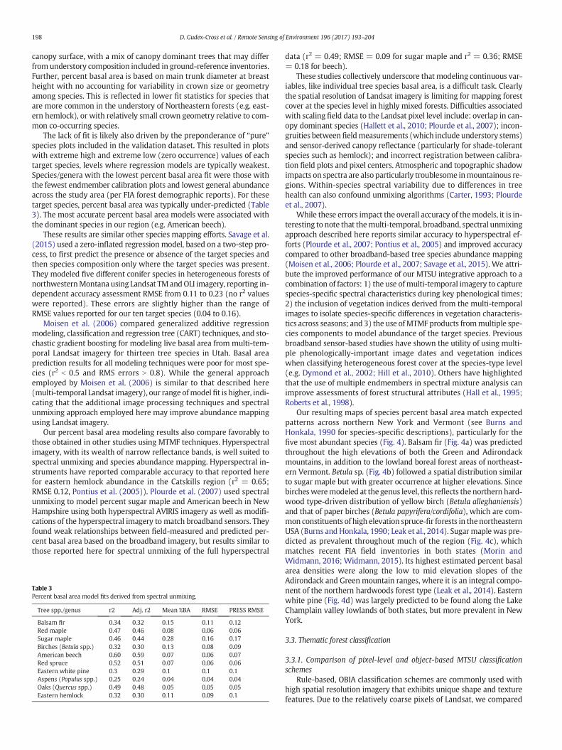
Our resulting maps of species percent basal area match expectedpatterns across northern New York and Vermont (see Burns andHonkala, 1990 for species-specific descriptions), particularly for thefive most abundant species (Fig. 4). Balsam fir (Fig. 4a) was predictedthroughout the high elevations of both the Green and Adirondackmountains, in addition to the lowland boreal forest areas of northeast-ern Vermont. Betula sp. (Fig. 4b) followed a spatial distribution similarto sugar maple but with greater occurrence at higher elevations. Sincebirchesweremodeled at the genus level, this reflects the northern hard-wood type-driven distribution of yellow birch (Betula alleghaniensis)and that of paper birches (Betula papyrifera/cordifolia), which are com-mon constituents of high elevation spruce-fir forests in thenortheasternUSA (Burns and Honkala, 1990; Leak et al., 2014). Sugar maple was pre-dicted as prevalent throughout much of the region (Fig. 4c), whichmatches recent FIA field inventories in both states (Morin andWidmann, 2016; Widmann, 2015). Its highest estimated percent basalarea densities were along the low to mid elevation slopes of theAdirondack and Greenmountain ranges, where it is an integral compo-nent of the northern hardwoods forest type (Leak et al., 2014). Easternwhite pine (Fig. 4d) was largely predicted to be found along the LakeChamplain valley lowlands of both states, but more prevalent in NewYork.

3.3. Thematic forest classification

3.3.1. Comparison of pixel-level and object-based MTSU classificationschemes

Rule-based, OBIA classification schemes are commonly used withhigh spatial resolution imagery that exhibits unique shape and texturefeatures. Due to the relatively coarse pixels of Landsat, we compared

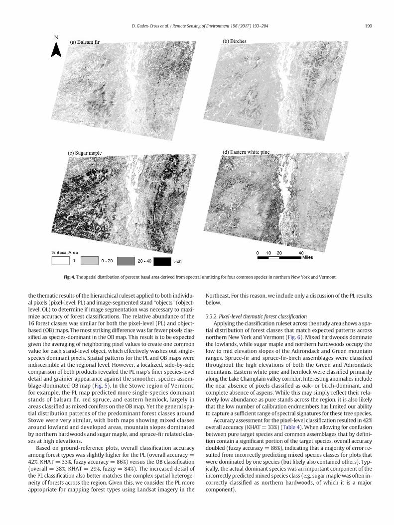
Fig. 4. The spatial distribution of percent basal area derived from spectral unmixing for four common species in northern New York and Vermont.

199D. Gudex-Cross et al. / Remote Sensing of Environment 196 (2017) 193–204

the thematic results of the hierarchical ruleset applied to both individu-al pixels (pixel-level, PL) and image-segmented stand “objects” (object-level, OL) to determine if image segmentation was necessary to maxi-mize accuracy of forest classifications. The relative abundance of the16 forest classes was similar for both the pixel-level (PL) and object-based (OB)maps. Themost striking differencewas far fewer pixels clas-sified as species-dominant in the OB map. This result is to be expectedgiven the averaging of neighboring pixel values to create one commonvalue for each stand-level object, which effectively washes out single-species dominant pixels. Spatial patterns for the PL and OB maps wereindiscernible at the regional level. However, a localized, side-by-sidecomparison of both products revealed the PL map's finer species-leveldetail and grainier appearance against the smoother, species assem-blage-dominated OB map (Fig. 5). In the Stowe region of Vermont,for example, the PL map predicted more single-species dominantstands of balsam fir, red spruce, and eastern hemlock, largely inareas classified as mixed conifers on the OBmap. Yet the general spa-tial distribution patterns of the predominant forest classes aroundStowe were very similar, with both maps showing mixed classesaround lowland and developed areas, mountain slopes dominatedby northern hardwoods and sugar maple, and spruce-fir related clas-ses at high elevations.

Based on ground-reference plots, overall classification accuracyamong forest types was slightly higher for the PL (overall accuracy =42%, KHAT = 33%, fuzzy accuracy = 86%) versus the OB classification(overall = 38%, KHAT = 29%, fuzzy = 84%). The increased detail ofthe PL classification also better matches the complex spatial heteroge-neity of forests across the region. Given this, we consider the PL moreappropriate for mapping forest types using Landsat imagery in the

Northeast. For this reason, we include only a discussion of the PL resultsbelow.

3.3.2. Pixel-level thematic forest classificationApplying the classification ruleset across the study area shows a spa-

tial distribution of forest classes that match expected patterns acrossnorthern New York and Vermont (Fig. 6). Mixed hardwoods dominatethe lowlands, while sugar maple and northern hardwoods occupy thelow to mid elevation slopes of the Adirondack and Green mountainranges. Spruce-fir and spruce-fir-birch assemblages were classifiedthroughout the high elevations of both the Green and Adirondackmountains. Eastern white pine and hemlock were classified primarilyalong the Lake Champlain valley corridor. Interesting anomalies includethe near absence of pixels classified as oak- or birch-dominant, andcomplete absence of aspens. While this may simply reflect their rela-tively low abundance as pure stands across the region, it is also likelythat the low number of calibration endmembers has limited our abilityto capture a sufficient range of spectral signatures for these tree species.

Accuracy assessment for the pixel-level classification resulted in 42%overall accuracy (KHAT= 33%) (Table 4). When allowing for confusionbetween pure target species and common assemblages that by defini-tion contain a significant portion of the target species, overall accuracydoubled (fuzzy accuracy = 86%), indicating that a majority of error re-sulted from incorrectly predicting mixed species classes for plots thatwere dominated by one species (but likely also contained others). Typ-ically, the actual dominant species was an important component of theincorrectly predictedmixed species class (e.g. sugarmaplewas often in-correctly classified as northern hardwoods, of which it is a majorcomponent).

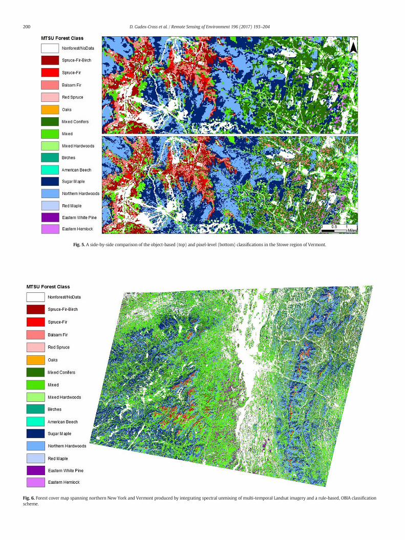
Fig. 6. Forest cover map spanning northern New York and Vermont produced by integrating spectral unmixing of multi-temporal Landsat imagery and a rule-based, OBIA classificationscheme.

Fig. 5. A side-by-side comparison of the object-based (top) and pixel-level (bottom) classifications in the Stowe region of Vermont.

200 D. Gudex-Cross et al. / Remote Sensing of Environment 196 (2017) 193–204

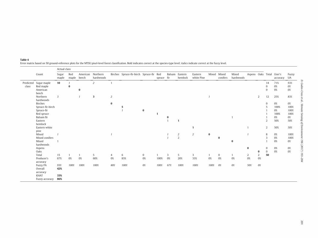
Table 4Error matrix based on 50 ground-reference plots for the MTSU pixel-level forest classification. Bold indicates correct at the species-type level; italics indicate correct at the fuzzy level.

Actual class

Count Sugarmaple

Redmaple

Americanbeech

Northernhardwoods

Birches Spruce-fir-birch Spruce-fir Redspruce

Balsamfir

Easternhemlock

Easternwhite Pine

Mixed Mixedconifers

Mixedhardwoods

Aspens Oaks Total User'saccuracy

FuzzyUA

Predictedclass

Sugar maple 10 1 2 1 14 71% 93%Red maple 0 0 0% 0%Americanbeech

0 0 0% 0%

Northernhardwoods

3 1 3 2 1 2 12 25% 83%

Birches 0 0 0% 0%Spruce-fir-birch 5 5 100% 100%Spruce-fir 1 0 1 0% 100%Red spruce 1 1 100% 100%Balsam fir 0 1 1 0% 0%Easternhemlock

1 1 2 50% 50%

Eastern whitepine

1 1 2 50% 50%

Mixed 1 1 1 2 2 0 1 8 0% 100%Mixed conifers 1 2 0 3 0% 100%Mixedhardwoods

1 0 1 0% 0%

Aspens 0 0 0% 0%Oaks 0 0 0% 0%Total 15 1 1 5 4 6 0 1 3 5 3 1 0 1 2 2 50Producer'saccuracy

67% 0% 0% 60% 0% 83% 0% 100% 0% 20% 33% 0% 0% 0% 0% 0%

Fuzzy PA 93% 100% 100% 100% 80% 100% 0% 100% 67% 100% 100% 100% 0% 0% 50% 0%Overallaccuracy

42%

KHAT 33%Fuzzy accuracy 86%

201D.G

udex-Crossetal./Rem

oteSensing

ofEnvironment196

(2017)193–204

202 D. Gudex-Cross et al. / Remote Sensing of Environment 196 (2017) 193–204

The highest producer's accuracies were obtained for the most com-mon forest types across the study area (Table 4): sugarmaple, northernhardwoods, and spruce-fir-birch. Lower user's accuracies for northernhardwoods highlight the tendency of the ruleset to categorize singlespecies-dominant validation plots into this species assemblage class.The lowest user's accuracies were obtained for less common specieswith relatively low abundance across the study area. These includedbirches and the three conifer species (balsam fir, eastern hemlock, andeastern white pine), all of which were often classified as mixed speciesassemblages. If identification of less abundant species is desired, thepercent basal area thresholds of the ruleset could be lowered to denote“dominant stands”. However, we suggest that if the goal of using theseforestmaps is examining the spatial and structural distribution of a par-ticular species, using the percent basal area maps themselves would bepreferential to using the thematic classification.

3.3.3. Comparison to other forest mapping productsIn order to evaluate how this integrated forest classification com-

pared to other commonly used forest covermaps, we consider the spec-ificity of forest classes (number and structure of distinct classes), thespatial resolution, and the mapping accuracy of each product (Table 5).

Our forest classification resulted in 15 forest types (no aspen standsmapped) across the study area, based on the 10 most common genera/species in the region and six common assemblages of these species. TheNational Forest Type Map and LANDFIRE EVT forest class structures aremost comparable to our MTSU integrated classification with 29 and 17predicted across the study area. Both include common species assem-blages such as spruce-fir and northern hardwoods. The National ForestType Map also includes species-specific classes (e.g. balsam fir, easternhemlock, eastern white pine, etc.). Where the LANDFIRE EVT classifica-tion diverges from ours is in its use of disturbance and geographic mod-ifiers to describe certain forest types (e.g. ruderal forest, Atlantic swampforest). Further, its mixed forest classes often cover a broader range ofspecies assemblages, (e.g. pine-hemlock-hardwood and spruce-fir-hardwood). The NLCD product only classifies three broad forest types:deciduous, evergreen, and mixed.

Our 50 ground-reference plots represented 11 forest types for ourMTSU integrated classification, five for the LANDFIRE EVT, and six forthe National Forest Type Map (Table 5). Of the five LANDFIRE EVT clas-ses, nearly all were predicted as belonging to one of three mixed foresttypes (pine-hemlock-hardwood, spruce-fir-hardwood, or yellow birch-sugar maple). Of the six National Forest Type Map classes, our ground-reference plots were predominantly categorized as one mixed foresttype (sugar maple-beech-yellow birch). This simplification of the het-erogeneity of species assemblages found across the Northern Forest re-gion into broad categories resulted in a gross over-prediction of yellowbirch-sugar maple (LANDFIRE EVT) and sugar maple-beech-yellowbirch (National Forest Type Map) across the landscape, while missingother species entirely.

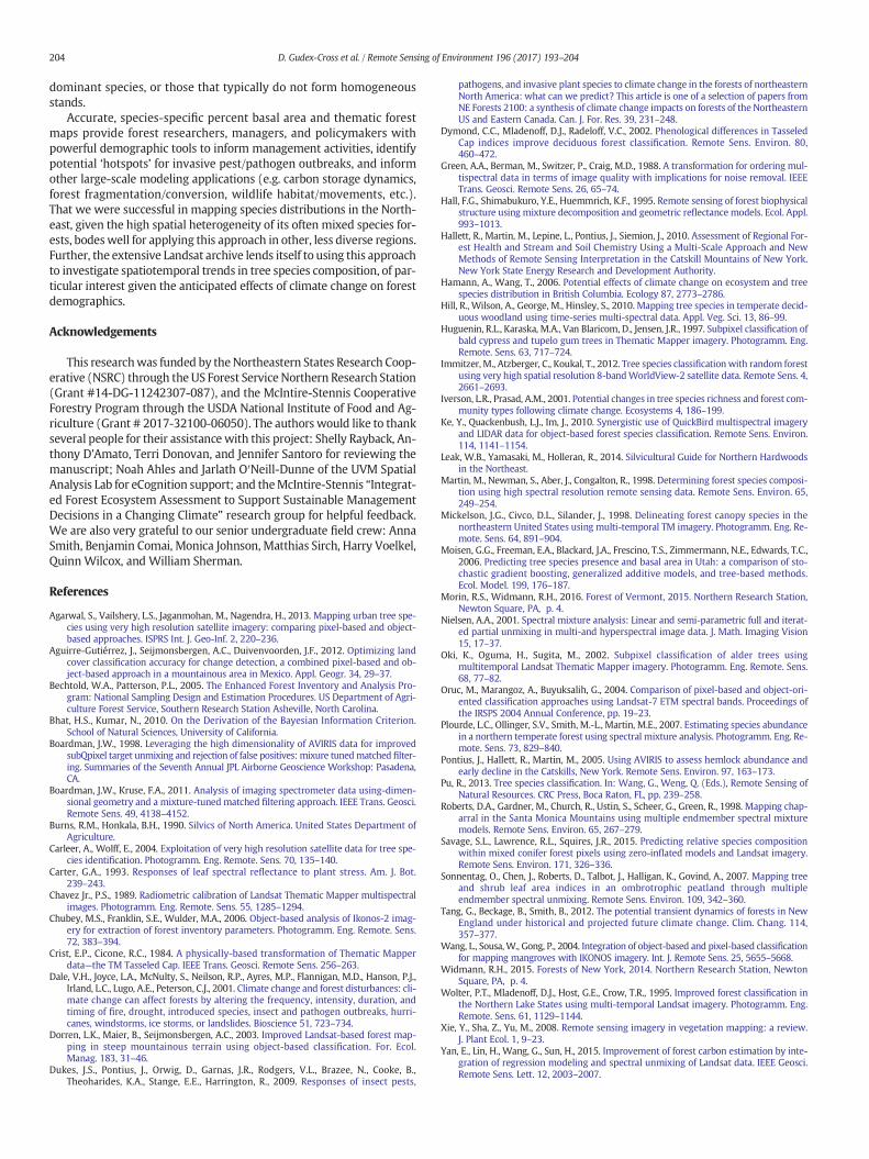
Focusing on the topographically diverse forests in the Stowe regionof Vermont, a comparison of these forest classifications highlights theincreased spatial detail and specificity of our MTSU product (Fig. 7).The MTSU predicts balsam fir, red spruce, spruce-fir, and spruce-fir-birch stands at high elevations, in addition to scattered balsam fir dom-inated stands in lowland swamp areas near suburban developments.Along mountain slopes, northern hardwoods and sugar maple standsare found throughout the low-mid elevations, with rare occurrences

Table 5Comparison of class specificity, spatial resolution, and accuracy of forest mapping products.

Product # Forest classes Spatial resolution (m)

MTSU 15 30LANDFIRE 17 30National forest type map 29 250NLCD 3 30

of birch and American beech dominated pixels. The valleys are largelydominated by the MTSU's broadest species assemblages: mixed,mixed conifers, and mixed hardwoods. These results contrast those ofthe National Forest Type Map and LANDFIRE EVT, which both classifymuch of the region as a mixed northern hardwoods-type (maple/beech/birch and yellow birch-sugar maple, respectively). The NationalForest TypeMap also does poorly distinguishing forest from non-forest,and has amore pixelated appearance due to its coarse spatial resolution.The spatial distribution of NLCD forest cover aligns most closely withthat of the MTSU product, but at a much coarser forest type specificity.

To compare accuracy among the mapping products, we used thesame 50 ground-reference plots referenced throughout this study.Since there are inherent differences in how each product categorizesforest types, ground-reference plots were assigned to match the com-parison product categories based on their species composition. Our re-sults indicate that our MTSU classification was more accurate than theLANDFIRE EVT product (42% compared to 28% overall accuracy respec-tively) and more than twice as accurate as the National Forest TypeMap (42% compared to 18% overall accuracy respectively) (Table 5).While fuzzy accuracies are improved for the National Forest Type Mapand LANDFIRE EVT products, this is likely inflated by their broad classstructure and near uniform assignment of plots into mixed forest typeclasses that include most of the common species/genera found withinour ground-reference dataset.

When modifying all four classifications to match the coarser NLCDforest types (i.e. deciduous, evergreen, and mixed forest) for a more di-rect comparison of the general performance of these models, again theMTSU outperformed the LANDFIRE EVT, National Forest Type Map,andNLCD products (76%, 66%, 62% and 56% overall accuracy, respective-ly) (Table 5). Most of the error in the MTSU was due to an over-predic-tion of mixed forest in conifer dominated plots. Deciduous forest, by farthemost common class in the ground-reference data, was also themostaccurately predicted in each classification. The high deciduous class ac-curacies of the LANDFIRE EVT and National Forest TypeMapwere againdriven by their propensity to predict yellow birch-sugar maple andsugar maple-beech-yellow birch across the landscape.

4. Conclusions

Our results indicate that the use of multi-temporal Landsat imagery,spectral unmixing, and a hierarchical ruleset classification (‘MTSU’ inte-grated approach) offers improved species specificity and accuracy rela-tive to existing forest classification products. The key to this approachincludes: 1) the use of multi-temporal imagery to capture species-spe-cific differences during important phenological periods; 2) spectralunmixing tomore accurately characterize themixed composition of for-ests in the study area; and 3) integration of resulting percent basal areamaps and ancillary environmental variables into a hierarchical, rule-based classification scheme.

Public availability of Landsat and FIA data enable the broad imple-mentation, as well as scalable nature, of this approach. However, it isimportant to note that this approach hinges upon the user's ability toobtain high quality (low cloud cover) multi-temporal imagery duringkey phenological periods, which is often difficult in temperate andmountainous regions. It also requires a robust set of “pure” speciesplots for use as endmembers in spectral unmixing and calibration ofthe percent basal area models. This can be difficult for rare and non-

Spp-type accuracy Fuzzy accuracy NLCD coarse accuracy

42% 86% 76%28% 80% 66%18% 70% 62%– – 56%

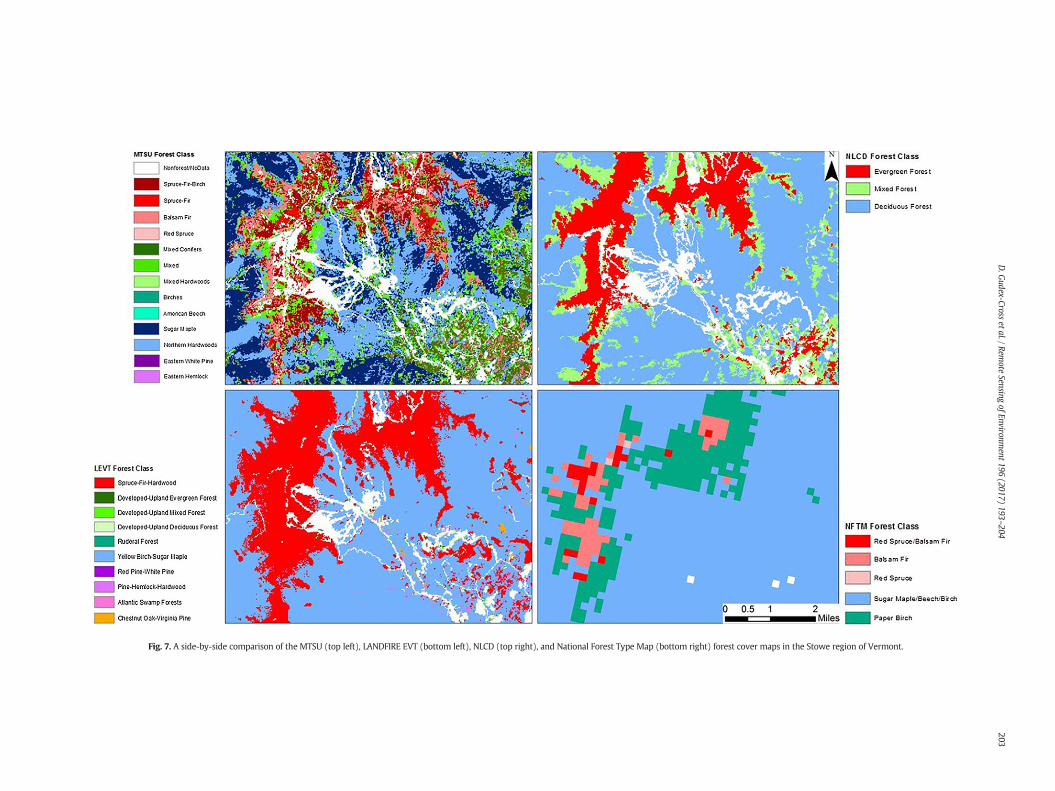
Fig. 7. A side-by-side comparison of the MTSU (top left), LANDFIRE EVT (bottom left), NLCD (top right), and National Forest Type Map (bottom right) forest cover maps in the Stowe region of Vermont.

203D.G

udex-Crossetal./Rem

oteSensing

ofEnvironment196

(2017)193–204

204 D. Gudex-Cross et al. / Remote Sensing of Environment 196 (2017) 193–204

dominant species, or those that typically do not form homogeneousstands.

Accurate, species-specific percent basal area and thematic forestmaps provide forest researchers, managers, and policymakers withpowerful demographic tools to inform management activities, identifypotential ‘hotspots’ for invasive pest/pathogen outbreaks, and informother large-scale modeling applications (e.g. carbon storage dynamics,forest fragmentation/conversion, wildlife habitat/movements, etc.).That we were successful in mapping species distributions in the North-east, given the high spatial heterogeneity of its often mixed species for-ests, bodeswell for applying this approach in other, less diverse regions.Further, the extensive Landsat archive lends itself to using this approachto investigate spatiotemporal trends in tree species composition, of par-ticular interest given the anticipated effects of climate change on forestdemographics.

Acknowledgements

This researchwas funded by theNortheastern States Research Coop-erative (NSRC) through the US Forest Service Northern Research Station(Grant #14-DG-11242307-087), and the McIntire-Stennis CooperativeForestry Program through the USDA National Institute of Food and Ag-riculture (Grant # 2017-32100-06050). The authors would like to thankseveral people for their assistance with this project: Shelly Rayback, An-thony D'Amato, Terri Donovan, and Jennifer Santoro for reviewing themanuscript; Noah Ahles and Jarlath O′Neill-Dunne of the UVM SpatialAnalysis Lab for eCognition support; and theMcIntire-Stennis “Integrat-ed Forest Ecosystem Assessment to Support Sustainable ManagementDecisions in a Changing Climate” research group for helpful feedback.We are also very grateful to our senior undergraduate field crew: AnnaSmith, Benjamin Comai, Monica Johnson, Matthias Sirch, Harry Voelkel,Quinn Wilcox, and William Sherman.

References

Agarwal, S., Vailshery, L.S., Jaganmohan, M., Nagendra, H., 2013. Mapping urban tree spe-cies using very high resolution satellite imagery: comparing pixel-based and object-based approaches. ISPRS Int. J. Geo-Inf. 2, 220–236.

Aguirre-Gutiérrez, J., Seijmonsbergen, A.C., Duivenvoorden, J.F., 2012. Optimizing landcover classification accuracy for change detection, a combined pixel-based and ob-ject-based approach in a mountainous area in Mexico. Appl. Geogr. 34, 29–37.

Bechtold, W.A., Patterson, P.L., 2005. The Enhanced Forest Inventory and Analysis Pro-gram: National Sampling Design and Estimation Procedures. US Department of Agri-culture Forest Service, Southern Research Station Asheville, North Carolina.

Bhat, H.S., Kumar, N., 2010. On the Derivation of the Bayesian Information Criterion.School of Natural Sciences, University of California.

Boardman, J.W., 1998. Leveraging the high dimensionality of AVIRIS data for improvedsubQpixel target unmixing and rejection of false positives: mixure tunedmatched filter-ing. Summaries of the Seventh Annual JPL Airborne Geoscience Workshop: Pasadena,CA.

Boardman, J.W., Kruse, F.A., 2011. Analysis of imaging spectrometer data using-dimen-sional geometry and a mixture-tuned matched filtering approach. IEEE Trans. Geosci.Remote Sens. 49, 4138–4152.

Burns, R.M., Honkala, B.H., 1990. Silvics of North America. United States Department ofAgriculture.

Carleer, A., Wolff, E., 2004. Exploitation of very high resolution satellite data for tree spe-cies identification. Photogramm. Eng. Remote. Sens. 70, 135–140.

Carter, G.A., 1993. Responses of leaf spectral reflectance to plant stress. Am. J. Bot.239–243.

Chavez Jr., P.S., 1989. Radiometric calibration of Landsat Thematic Mapper multispectralimages. Photogramm. Eng. Remote. Sens. 55, 1285–1294.

Chubey, M.S., Franklin, S.E., Wulder, M.A., 2006. Object-based analysis of Ikonos-2 imag-ery for extraction of forest inventory parameters. Photogramm. Eng. Remote. Sens.72, 383–394.

Crist, E.P., Cicone, R.C., 1984. A physically-based transformation of Thematic Mapperdata—the TM Tasseled Cap. IEEE Trans. Geosci. Remote Sens. 256–263.

Dale, V.H., Joyce, L.A., McNulty, S., Neilson, R.P., Ayres, M.P., Flannigan, M.D., Hanson, P.J.,Irland, L.C., Lugo, A.E., Peterson, C.J., 2001. Climate change and forest disturbances: cli-mate change can affect forests by altering the frequency, intensity, duration, andtiming of fire, drought, introduced species, insect and pathogen outbreaks, hurri-canes, windstorms, ice storms, or landslides. Bioscience 51, 723–734.

Dorren, L.K., Maier, B., Seijmonsbergen, A.C., 2003. Improved Landsat-based forest map-ping in steep mountainous terrain using object-based classification. For. Ecol.Manag. 183, 31–46.

Dukes, J.S., Pontius, J., Orwig, D., Garnas, J.R., Rodgers, V.L., Brazee, N., Cooke, B.,Theoharides, K.A., Stange, E.E., Harrington, R., 2009. Responses of insect pests,

pathogens, and invasive plant species to climate change in the forests of northeasternNorth America: what can we predict? This article is one of a selection of papers fromNE Forests 2100: a synthesis of climate change impacts on forests of the NortheasternUS and Eastern Canada. Can. J. For. Res. 39, 231–248.

Dymond, C.C., Mladenoff, D.J., Radeloff, V.C., 2002. Phenological differences in TasseledCap indices improve deciduous forest classification. Remote Sens. Environ. 80,460–472.

Green, A.A., Berman, M., Switzer, P., Craig, M.D., 1988. A transformation for ordering mul-tispectral data in terms of image quality with implications for noise removal. IEEETrans. Geosci. Remote Sens. 26, 65–74.

Hall, F.G., Shimabukuro, Y.E., Huemmrich, K.F., 1995. Remote sensing of forest biophysicalstructure using mixture decomposition and geometric reflectance models. Ecol. Appl.993–1013.

Hallett, R., Martin, M., Lepine, L., Pontius, J., Siemion, J., 2010. Assessment of Regional For-est Health and Stream and Soil Chemistry Using a Multi-Scale Approach and NewMethods of Remote Sensing Interpretation in the Catskill Mountains of New York.New York State Energy Research and Development Authority.

Hamann, A., Wang, T., 2006. Potential effects of climate change on ecosystem and treespecies distribution in British Columbia. Ecology 87, 2773–2786.

Hill, R., Wilson, A., George, M., Hinsley, S., 2010. Mapping tree species in temperate decid-uous woodland using time-series multi-spectral data. Appl. Veg. Sci. 13, 86–99.

Huguenin, R.L., Karaska, M.A., Van Blaricom, D., Jensen, J.R., 1997. Subpixel classification ofbald cypress and tupelo gum trees in Thematic Mapper imagery. Photogramm. Eng.Remote. Sens. 63, 717–724.

Immitzer, M., Atzberger, C., Koukal, T., 2012. Tree species classificationwith random forestusing very high spatial resolution 8-bandWorldView-2 satellite data. Remote Sens. 4,2661–2693.

Iverson, L.R., Prasad, A.M., 2001. Potential changes in tree species richness and forest com-munity types following climate change. Ecosystems 4, 186–199.

Ke, Y., Quackenbush, L.J., Im, J., 2010. Synergistic use of QuickBird multispectral imageryand LIDAR data for object-based forest species classification. Remote Sens. Environ.114, 1141–1154.

Leak, W.B., Yamasaki, M., Holleran, R., 2014. Silvicultural Guide for Northern Hardwoodsin the Northeast.

Martin, M., Newman, S., Aber, J., Congalton, R., 1998. Determining forest species composi-tion using high spectral resolution remote sensing data. Remote Sens. Environ. 65,249–254.

Mickelson, J.G., Civco, D.L., Silander, J., 1998. Delineating forest canopy species in thenortheastern United States using multi-temporal TM imagery. Photogramm. Eng. Re-mote. Sens. 64, 891–904.

Moisen, G.G., Freeman, E.A., Blackard, J.A., Frescino, T.S., Zimmermann, N.E., Edwards, T.C.,2006. Predicting tree species presence and basal area in Utah: a comparison of sto-chastic gradient boosting, generalized additive models, and tree-based methods.Ecol. Model. 199, 176–187.

Morin, R.S., Widmann, R.H., 2016. Forest of Vermont, 2015. Northern Research Station,Newton Square, PA, p. 4.

Nielsen, A.A., 2001. Spectral mixture analysis: Linear and semi-parametric full and iterat-ed partial unmixing in multi-and hyperspectral image data. J. Math. Imaging Vision15, 17–37.

Oki, K., Oguma, H., Sugita, M., 2002. Subpixel classification of alder trees usingmultitemporal Landsat Thematic Mapper imagery. Photogramm. Eng. Remote. Sens.68, 77–82.

Oruc, M., Marangoz, A., Buyuksalih, G., 2004. Comparison of pixel-based and object-ori-ented classification approaches using Landsat-7 ETM spectral bands. Proceedings ofthe IRSPS 2004 Annual Conference, pp. 19–23.

Plourde, L.C., Ollinger, S.V., Smith, M.-L., Martin, M.E., 2007. Estimating species abundancein a northern temperate forest using spectral mixture analysis. Photogramm. Eng. Re-mote. Sens. 73, 829–840.

Pontius, J., Hallett, R., Martin, M., 2005. Using AVIRIS to assess hemlock abundance andearly decline in the Catskills, New York. Remote Sens. Environ. 97, 163–173.

Pu, R., 2013. Tree species classification. In: Wang, G., Weng, Q. (Eds.), Remote Sensing ofNatural Resources. CRC Press, Boca Raton, FL, pp. 239–258.

Roberts, D.A., Gardner, M., Church, R., Ustin, S., Scheer, G., Green, R., 1998. Mapping chap-arral in the Santa Monica Mountains using multiple endmember spectral mixturemodels. Remote Sens. Environ. 65, 267–279.

Savage, S.L., Lawrence, R.L., Squires, J.R., 2015. Predicting relative species compositionwithin mixed conifer forest pixels using zero-inflated models and Landsat imagery.Remote Sens. Environ. 171, 326–336.

Sonnentag, O., Chen, J., Roberts, D., Talbot, J., Halligan, K., Govind, A., 2007. Mapping treeand shrub leaf area indices in an ombrotrophic peatland through multipleendmember spectral unmixing. Remote Sens. Environ. 109, 342–360.

Tang, G., Beckage, B., Smith, B., 2012. The potential transient dynamics of forests in NewEngland under historical and projected future climate change. Clim. Chang. 114,357–377.

Wang, L., Sousa,W., Gong, P., 2004. Integration of object-based and pixel-based classificationfor mapping mangroves with IKONOS imagery. Int. J. Remote Sens. 25, 5655–5668.

Widmann, R.H., 2015. Forests of New York, 2014. Northern Research Station, NewtonSquare, PA, p. 4.

Wolter, P.T., Mladenoff, D.J., Host, G.E., Crow, T.R., 1995. Improved forest classification inthe Northern Lake States using multi-temporal Landsat imagery. Photogramm. Eng.Remote. Sens. 61, 1129–1144.

Xie, Y., Sha, Z., Yu, M., 2008. Remote sensing imagery in vegetation mapping: a review.J. Plant Ecol. 1, 9–23.

Yan, E., Lin, H., Wang, G., Sun, H., 2015. Improvement of forest carbon estimation by inte-gration of regression modeling and spectral unmixing of Landsat data. IEEE Geosci.Remote Sens. Lett. 12, 2003–2007.