remote sensing of soil moisture using airborne ... sensing of soil moisture using airborne...

522

GIScience & Remote Sensing, 2011, 48, No. 4, p. 522–540. http://dx.doi.org/10.2747/1548-1603.48.4.522Copyright © 2011 by Bellwether Publishing, Ltd. All rights reserved.

Remote Sensing of Soil Moisture Using Airborne Hyperspectral Data1

Michael P. Finn2 U.S. Geological Survey (USGS), Center of Excellence for Geospatial Information Science (CEGIS), Denver Federal Center, Box 25046, Mail Stop 510, Denver, Colorado 80225

Mark (David) Lewis3

Institute for Technology Development (ITD) Stennis Space Center, Mississippi 39529

David D. BoschU. S. Department of Agriculture–Agricultural Research Service (USDA-ARS), Southeast Watershed Research Laboratory (SEWRL), P.O. Box 748 Tifton, Georgia 31793

Mario Giraldo4 Department of Geography, University of Georgia, Athens, Georgia 30602

Kristina YamamotoU.S. Geological Survey (USGS), Center of Excellence for Geospatial Information Science (CEGIS), Denver Federal Center, Box 25046, Mail Stop 510, Denver, Colorado 80225

Dana G. Sullivan5 U. S. Department of Agriculture–Agricultural Research Service (USDA-ARS), Southeast Watershed Research Laboratory (SEWRL), P.O. Box 748 Tifton, Georgia 31792

Russell KincaidInstitute for Technology Development (ITD) Stennis Space Center, Mississippi 39529

1Any use of trade names in this publication is for descriptive purposes only and does not constitute endorsement by the U.S. Government.2Corresponding author; email: [email protected] with Naval Research Laboratory, Building 1009, Room A128, Stennis Space Center, MS 39529.4Now with Kennesaw State University, Kennesaw, Georgia.5Now with Turfscout LLC.

remote sensing of soil moisture 523

Ronaldo Luna and Gopala Krishna Allam6 Missouri University of Science and Technology (Missouri S&T), Department of Civil, Architectural, and Environmental Engineering, Rolla, Missouri 65409

Craig KvienUniversity of Georgia, National Environmentally Sound Production Agricultural Laboratory (NESPAL), Tifton, Georgia 31793

Michael S. Williams7

U.S. Geological Survey, Center of Excellence for Geospatial Information Science (CEGIS), Rolla, Missouri 65401

Abstract: Landscape assessment of soil moisture is critical to understanding the hydrological cycle at the regional scale and in broad-scale studies of biophysi-cal processes affected by global climate changes in temperature and precipitation. Traditional efforts to measure soil moisture have been principally restricted to in situ measurements, so remote sensing techniques are often employed. Hyperspectral sensors with finer spatial resolution and narrow band widths may offer an alternative to traditional multispectral analysis of soil moisture, particularly in landscapes with high spatial heterogeneity. This preliminary research evaluates the ability of remotely sensed hyperspectral data to quantify soil moisture for the Little River Experimental Watershed (LREW), Georgia. An airborne hyperspectral instrument with a short-wavelength infrared (SWIR) sensor was flown in 2005 and 2007 and the results were correlated to in situ soil moisture values. A significant statistical correlation (R2 value above 0.7 for both sampling dates) for the hyperspectral instrument data and the soil moisture probe data at 5.08 cm (2 inches) was determined. While models for the 20.32 cm (8 inches) and 30.48 cm (12 inches) depths were tested, they were not able to estimate soil moisture to the same degree.

INTRODUCTION

Soil moisture is a critical process in the water cycle and its assessment is of para-mount importance in forecasting changes in the water balance of a region (Salvucci et al., 2002). In agricultural production, the spatial variability of soil moisture can be responsible for low or spatially variable crop yields, as soil moisture is required to make nutrients soluble for plant absorption.

Soil moisture fluctuates both spatially and temporally due to factors such as soil type, soil horizon, and other site-specific geologic and climatic conditions. Traditional efforts to measure soil moisture have been principally restricted to in situ measurements

6Now with Terracon Consultants, Inc., Omaha, Nebraska.7Now with Garmin International Inc., Olathe, Kansas.

524 finn et al.

(Engman, 1999) and predominately reliant on direct field instrumentation and point data (Steele-Dunne et al., 2010), which can be costly when used to obtain spatially distributed data over a large region or landscape (Jensen and Hodgson, 2004). As an alternative to ground point data, remote sensing data are seen as a promising approach to evaluate soil moisture characteristics in different landscapes and sampling areas by providing in a regional description of the water redistribution at different temporal and spatial resolutions (McCabe and Wood, 2006).

The advantage of remote digital imaging is that relatively frequent measurements can be made. By subtracting spatially referenced data, time-displacement associations (i.e., time series) can be produced. Beginning in the 1920s, aerial photographs were used to delineate and map boundaries of different soil series by identifying dissimilari-ties in photographs (Helms et al., 2002). By focusing primarily on using vegetation as a proxy for soil water holding capacity, mapped soils, derived from those image demarcations, can aid managers and farmers in identifying homogenous zones within agricultural fields for guiding nutrient application rates using variable rate technology (VRT) (Baumgardner et al., 1985; Walthall et al., 2001; Gish et al., 2002; Daughtry et al., 2002).

More recently, soil scientists have used multispectral images for mapping land cover attributes and related moisture conditions. The wetness in the top few centime-ters of soil can be measured remotely using multispectral remote sensing or certain radar bands (Njoku and Entekhabi, 1996). Transformations of the spectral reflectance in remotely sensed images can provide useful information on soil water content and, if augmented with existing soil and other geospatial information, can provide spatially representative estimates of soil moisture. Most studies using remotely sensed data to look for relationships with soil properties have focused on the 0.3 to 2.8 micrometer region of the electromagnetic spectrum (Bushnell, 1932; Barnes et al., 2003).

Despite numerous studies, a universal spectral range and sampling scheme has yet to be determined for best detecting soil moisture. Visible near-infrared (VNIR) (0.4–1.4 μm), near-infrared (NIR) (0.75–1.4 μm), short-wavelength infrared (SWIR) (1.4–3.0 μm), thermal infrared (3.5–20 μm), and microwave (0.3–300 cm) have each shown some promise. In general, the literature suggests that the longer the wavelength the better the potential ability to predict soil moisture. NIR appears to be a suitable option for bare-soil fields after a rainfall (Milfred and Kiefer, 1976) if the particle size and soil type are the same as the calibration set (Slaughter et al., 2001). NIR, when used in conjunction with visible bands, holds promise to categorize soil samples by moisture content, especially when soil variability is low (Mouazen et al., 2006). As a better alternative, SWIR has been shown to be more effective than VNIR at moni-toring soil moisture changes (important to predicting soil moisture), as long as the soil moisture values remain at less than or equal to 50% of volumetric water content (Lobell and Asner, 2002), especially the creation of Gaussian models for soils from the Mediterranean region (Whiting et al., 2004). Measurements from the thermal infrared portion of the electromagnetic spectrum have also been conducted. Thermal infrared emissivity increases as soil moisture content decreases at low water content levels (Mira et al., 2010) and thermal infrared images with high spatial resolution can be used to map soil moisture at a fine scale (Katra et al., 2006).

Microwave bands also have the capacity to measure soil moisture (Moran et al., 1998; Barnes et al., 2003) over a selection of topographic and vegetation cover


settings (Jackson et al., 1997). On relatively unvegetated soil it is possible to obtain reasonably accurate soil moisture estimates using active microwave X- (2.4–3.8 cm) and C-band (3.8–7.5 cm) radar imagery (Jensen et al., 2005). Because of the signal ability to penetrate the earth, microwave technology allows scientists to gather data on the properties of the zone from the soil surface to the groundwater table (Crow et al., 2005). Extending this technology to routine measurements from a satellite system would supply notable spatial and temporal characteristics to hydrologic measurements (Engman, 1999). Additional microwave remote sensing investigations specific to our study area are expanded upon in the next section of this paper.

As an alternative to broad-band multispectral remote sensing sensors, which collect spectral information across relatively wide ranges of the electromagnetic spec-trum, hyperspectral sensors collect remote sensing data as images, with each image representing a different spectral band with higher spectral resolution than broad-band sensors. When stacked together, the two-dimensional spatial (image) data sets create hyperspectral data cubes, with two dimensions containing spatial information and the third dimension containing spectral information (Warren et al., 1997; Vogt et al., 2004).

The possibilities of using hyperspectral data to obtain soil water content are still uncertain, but appear promising. For example, Grandjean et al., (2010) identified air-borne hyperspectral sensing as one of the anticipated geophysical sensor technologies that will aid the dilemma of performing soil data collections at the catchment scale. The use of airborne hyperspectral sensing will bridge a technological gap for the purpose of developing steadfast and cost-effective geophysical mapping solutions, especially for data collection in digital soil property mapping (soil texture, soil water content, soil hydraulic properties, bulk density, and soil organic matter). While airplane-mounted sensors have distinct advantages over satellite-based systems, the approach has yet to be thoroughly tested. The ability to have data with finer spatial resolution and more control over temporal resolution from aircraft mounted sensors is an advantage over satellite-based data. The larger ground area covered in less time is a benefit over in situ measurements.

OBJECTIVES

The purpose of this research was to test the statistical correlation between spectral bands of an airborne hyperspectral sensor and soil moisture ground readings at three different depths. The research explored whether the reflectance values available in hyperspectral remote sensing datasets can be used in the monitoring of soil water con-tent. This study contributes to an ongoing effort to obtain spatially accurate soil mois-ture data using remote sensors that can be used in hydrological and climatic research on such issues as drought prevention/risk, analyzing ground-atmosphere feedback, and crop irrigation techniques among others.

STUDY AREA

The Southeast Watershed Research Laboratory (SEWRL) of the U.S. Department of Agriculture has 30 instrumented stations continuously collecting soil water con-tent for the Little River Experimental Watershed (LREW), a small watershed in south

526 finn et al.

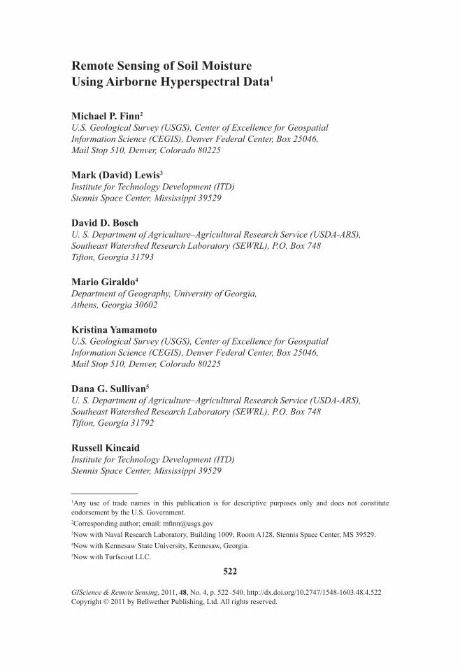
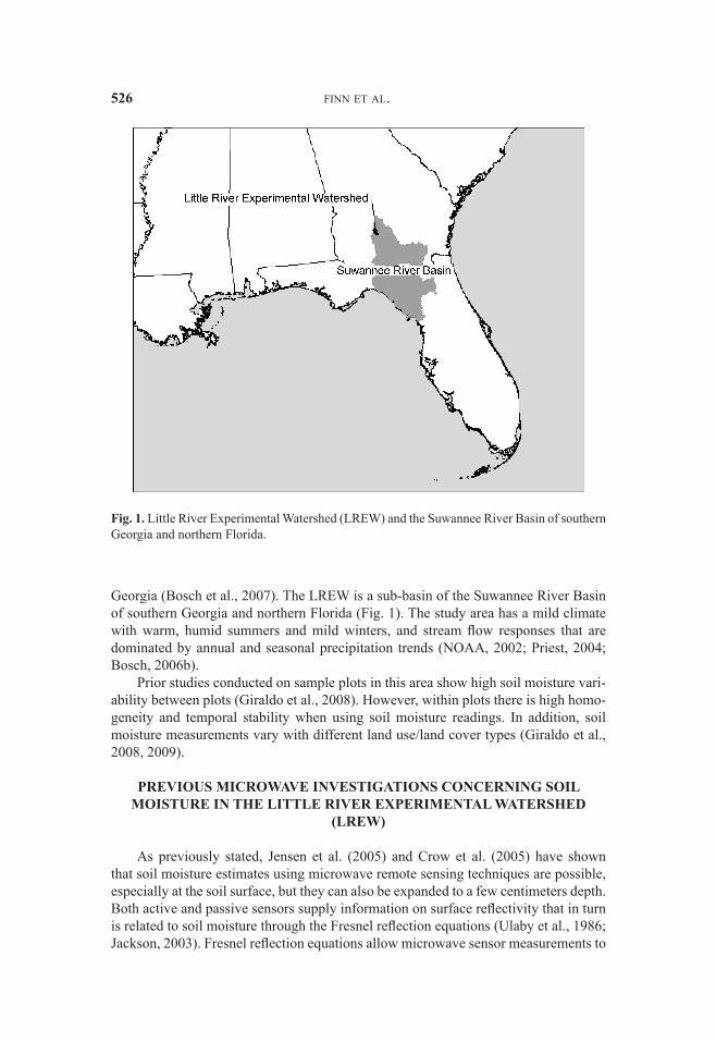
Georgia (Bosch et al., 2007). The LREW is a sub-basin of the Suwannee River Basin of southern Georgia and northern Florida (Fig. 1). The study area has a mild climate with warm, humid summers and mild winters, and stream flow responses that are dominated by annual and seasonal precipitation trends (NOAA, 2002; Priest, 2004; Bosch, 2006b).

Prior studies conducted on sample plots in this area show high soil moisture vari-ability between plots (Giraldo et al., 2008). However, within plots there is high homo-geneity and temporal stability when using soil moisture readings. In addition, soil moisture measurements vary with different land use/land cover types (Giraldo et al., 2008, 2009).

PREVIOUS MICROWAVE INVESTIGATIONS CONCERNING SOIL MOISTURE IN THE LITTLE RIVER EXPERIMENTAL WATERSHED

(LREW)

As previously stated, Jensen et al. (2005) and Crow et al. (2005) have shown that soil moisture estimates using microwave remote sensing techniques are possible, especially at the soil surface, but they can also be expanded to a few centimeters depth. Both active and passive sensors supply information on surface reflectivity that in turn is related to soil moisture through the Fresnel reflection equations (Ulaby et al., 1986; Jackson, 2003). Fresnel reflection equations allow microwave sensor measurements to

Fig. 1. Little River Experimental Watershed (LREW) and the Suwannee River Basin of southern Georgia and northern Florida.


be equated to soil moisture, based on relationships between reflected and transmitted electromagnetic waves.

Data were collected on the LREW using the National Oceanic and Atmospheric Administration (NOAA) Polarimetric Scanning Radiometer (PSR/CX) sensor during Soil Moisture Experiment 2003 SMEX03 (Jackson et al., 2005; Bosch et al., 2006a). The experiment was conducted over the LREW, Georgia, and sites in Oklahoma and Alabama. SMEX03 was the second in a chain of field campaigns conducted to validate brightness temperature data and soil moisture retrieval algorithms for the Advanced Microwave Scanning Radiometer for the Earth Observing System (AMSR-E) on the Aqua satellite. AMSR-E is a passive microwave radiometer sensing microwave radia-tion on 12 channels at six frequencies ranging from 6.9 to 89 GHz (0.3 to 4.3 cm). During SMEX03, researchers collected aircraft data with the PSR/CX sensor (X-Band, 2.5–3.7 cm wavelength with approximately 3 km spatial resolution), satellite AMSR-E X-Band (0.3–4.3 cm) data (40–75 km spatial resolution), and in situ measured soil moisture at 19 long-term sites and 49 supplemental sites (Jackson et al., 2005; Bosch et al., 2006a).

Jackson et al. (2005) found that both the PSR/CX and AMSR-E X-band channels were well calibrated and that X-band comparisons of the PSR/CX high-resolution data with the low-resolution data from AMSR-E indicated a linear scaling for the range of conditions studied in SMEX03. This work was followed by another analy-sis of AMSR-E in the LREW, where LREW and three other soil moisture networks were used (Jackson et al., 2010). They compared National Aeronautics and Space Administration (NASA) and Japan Aerospace Exploration Agency (JAXA) soil mois-ture products to the network observations, along with two alternative soil moisture products developed using the single-channel algorithm (SCA) and the land parameter retrieval model (LPRM). They found that the statistical results indicated that each algorithm performed differently at each site. Furthermore, the JAXA algorithm per-formed better than the NASA algorithm under light-vegetation conditions, whereas the NASA algorithm was more reliable for moderate vegetation. The SCA had the lowest overall root mean square error with a small bias, while the LPRM had a very large overestimation bias and retrieval errors.

Sahoo et al. (2008) estimated the soil moisture from AMSR-E using the 10.7 GHz (2.8 cm) frequency channel and compared it to the Land Surface Microwave Emission Model (LSMEM). In turn, they compared the two methods to in situ measured soil moisture datasets over the LREW and found that the LSMEM method performed bet-ter than the current operational AMSR-E retrieval algorithm.

DATA

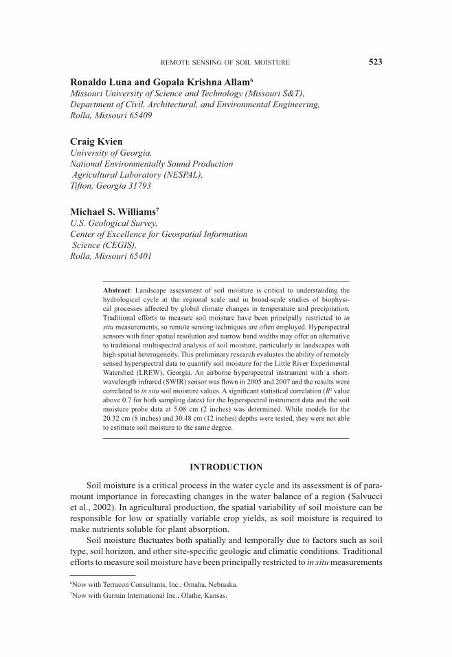
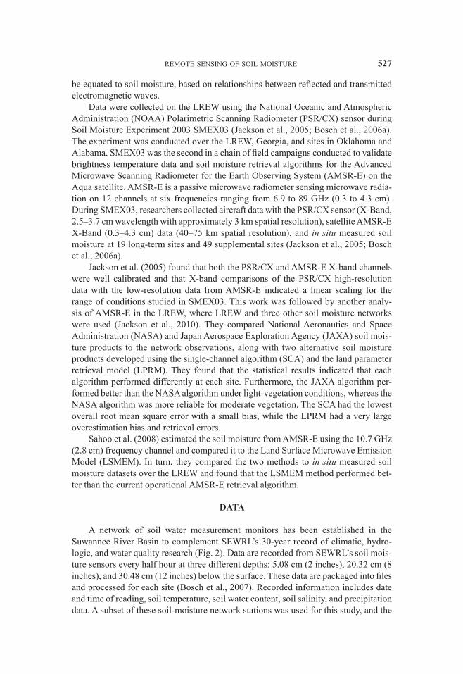
A network of soil water measurement monitors has been established in the Suwannee River Basin to complement SEWRL’s 30-year record of climatic, hydro-logic, and water quality research (Fig. 2). Data are recorded from SEWRL’s soil mois-ture sensors every half hour at three different depths: 5.08 cm (2 inches), 20.32 cm (8 inches), and 30.48 cm (12 inches) below the surface. These data are packaged into files and processed for each site (Bosch et al., 2007). Recorded information includes date and time of reading, soil temperature, soil water content, soil salinity, and precipitation data. A subset of these soil-moisture network stations was used for this study, and the

528 finn et al.

number of stations used was chosen to optimize hyperspectral data collection. Flights across the LREW were conducted on November 30, 2005 and March 6, 2007. For the November 30, 2005 flight, 18 soil moisture probes were chosen, and for the March 6, 2007 flight, 29 soil moisture probes were chosen.8 Flight lines were drawn over the selected soil moisture meters for each flight using United States Geological Survey (USGS) Digital Ortho Quads (DOQ).

The aircraft-mounted SWIR HyperSpectral Imaging (HSI) sensor, developed by the Institute for Technology Development (ITD) of the Stennis Space Center, was used to collect electromagnetic reflectance data over the soil moisture probe stations. The system consists of sensors for three different sections of the electromagnetic spectrum: ultraviolet (UV), VNIR, and SWIR. The sensor was mounted aboard a Cessna, which flew at a nominal 6,000 feet above the ground, resulting in a ground spatial resolu-tion of the image data at just over 6 meters. The extent of the image in the along-track direction was dictated by the distance the aircraft flew while the sensor was recording data. Flight lines were typically established by drawing multiple lines over a digital

8The first flight in 2005 was used to preliminarily test the feasibility of the project. Based on the results from the first flight, a more vigorous statistical design and analysis were conducted for the second flight in 2007.

Fig. 2. Locations of soil moisture sensors in the LREW.


map of the target area. The lines were oriented so that all the targets could be covered within the sensor’s field of view using the minimum number of flight lines. The lati-tude/ longitude of the start and stop points for each line were recorded. The start/stop and latitude/ longitude pairings were then uploaded into the GPS in the aircraft.

The ITD SWIR HSI sensor allows light to pass through a lens and enter into a spectrograph through a slit. The spectrograph in the sensor breaks light passing through the slit into wavelengths that are in the SWIR range. The resulting light illuminates a charge-coupled device (CCD) array and is dispersed with the shorter wavelengths illu-minating the top of the CCD array, and then gradually moving through the spectrum with the longer wavelengths illuminating the bottom of the CCD array.

The CCD array has 240 lines and 320 columns. The number of lines determines the maximum number of spectral bands that can be collected and the number of col-umns dictates the maximum number of cells of spatial information per line. With this SWIR CCD array, 240 lines of spectral band information could be obtained; however, for this research project, the number of photons that are collected in one 1 × 1 cell of the CCD array may not result in enough energy to excite the sensing element. To accommodate for this possibility, the sensor has the capability to aggregate several cells together. By increasing the number of cells that are aggregated together dur-ing data collection, a larger area can be created so that the accumulation of photons received by the combination of cells can increase the sensitivity for each recording element, thus improving the quality of the data.

Binning was used to aggregate cells to create a larger sensing element that records the number of detected photons for measurement. The two advantages to binning are: (1) it increases the signal to noise ratio for the data; and (2) binning the spatial dimen-sion increases the spatial resolution. Increasing the binning in the spectral dimension decreases the number of bands that is collected. For a sensor that collects a maximum of 240 spectral bands, a binning of the data by two causes the number of bands that is collected to be decreased by a factor of two, leaving 120 bands of data. Likewise, binning the data by four causes the data to be decreased by a factor of four, leaving 60 bands of data.

For the first flight on November 30, 2005, each of the 240 spectral sensing lines (elements) was binned with their neighbors to enhance the signal measurement. This resulted in every pair of the spectral sensing elements being binned together for data measurement and subsequently 120 bands of SWIR data were collected for each flight line in the image data. By binning spectrally instead of spatially, measurements of the spectral absorption troughs and reflection peaks were made while maintaining visual identification of the targets on the ground. High and low bands outside the spectral response of the spectrograph were omitted from the analysis. The resulting data set contained 85 bands of information with spectral response in the range of 937 to 1700 nanometers in wavelength.

For the second flight on March 6, 2007, four adjacent spectral sensing elements were binned together to further increase the signal measurement. This resulted in recording 60, or half, of the first flight’s number of spectral bands. All 60 bands of SWIR data were collected for each flight line in the image data. Again, the high and low bands outside the spectral response of the spectrograph were omitted from the analysis. Therefore, the data set that was used for analysis contained 43 bands of reflectance data with a wavelength range of 910 to 1686 nanometers.

530 finn et al.

The data for the second flight were corrected for atmospheric effects and system noise. Atmospheric correction is used to adjust for the absorption characteristics of the atmosphere and to convert the data to percent reflectance (Price, 1987; Chavez and Mackinnon, 1994). It uses a regression line with one graph point representing the raw digital number for the dark point on the x-axis and the corresponding percent reflectance of the radiometer data on the y-axis, while the other graph point represents the raw digital number for a bright point on the x-axis and the corresponding per-cent reflectance of the radiometer data on the y-axis. These regression equations were used to transform all the raw image data to percent reflectance. An Analytical Spectral Devices (ASD) SWIR radiometer was used to capture radiometric data for comparison with the hyperspectral data.

SWIR spectra were extracted from the radiometer data in percent reflectance units of measure and paired with SWIR spectra extracted from the noise-reduced image data to generate a regression equation for calibration. The linear regression equation from these pairings was used to transform all the image frames to percent reflectance. The resulting data sets contained bands with a spectral response between 910 to 1700 nanometers in wavelength.

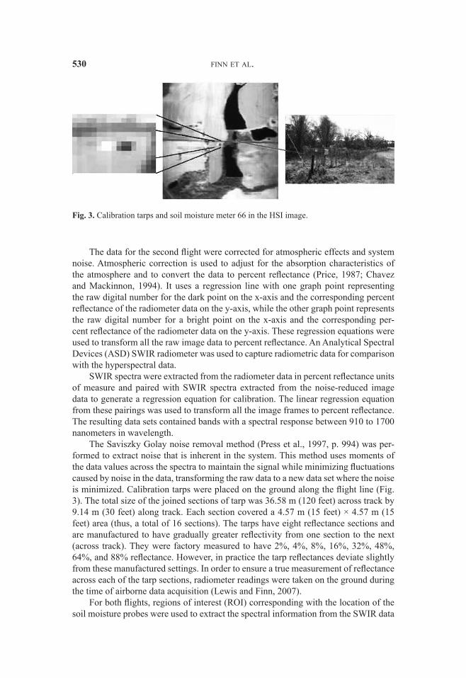
The Saviszky Golay noise removal method (Press et al., 1997, p. 994) was per-formed to extract noise that is inherent in the system. This method uses moments of the data values across the spectra to maintain the signal while minimizing fluctuations caused by noise in the data, transforming the raw data to a new data set where the noise is minimized. Calibration tarps were placed on the ground along the flight line (Fig. 3). The total size of the joined sections of tarp was 36.58 m (120 feet) across track by 9.14 m (30 feet) along track. Each section covered a 4.57 m (15 feet) × 4.57 m (15 feet) area (thus, a total of 16 sections). The tarps have eight reflectance sections and are manufactured to have gradually greater reflectivity from one section to the next (across track). They were factory measured to have 2%, 4%, 8%, 16%, 32%, 48%, 64%, and 88% reflectance. However, in practice the tarp reflectances deviate slightly from these manufactured settings. In order to ensure a true measurement of reflectance across each of the tarp sections, radiometer readings were taken on the ground during the time of airborne data acquisition (Lewis and Finn, 2007).

For both flights, regions of interest (ROI) corresponding with the location of the soil moisture probes were used to extract the spectral information from the SWIR data

Fig. 3. Calibration tarps and soil moisture meter 66 in the HSI image.


set for each of the soil moisture probe locations. Each ROI covers a 3 ×3 pixel mask around the soil moisture probe and the ground spatial resolution of the image data is just over 6 meters. Thus the ROI for each soil moisture probe is approximately 18 by 18 m. The 3 × 3 window of pixels within each ROI were then averaged to create one spectral value for each of the soil moisture probes. For the soil moisture probe data, the corresponding time of the HSI sensor data collection flight was used to obtain soil moisture values for the correlative soil moisture probes used. These sensor data for the 5.08 cm (2 inches), 20.32 cm (8 inches), and 30.48 cm (12 inches) probes were used for correlation to the SWIR spectral information.

ANALYSIS AND RESULTS

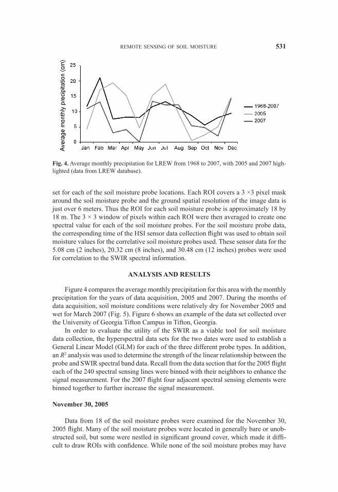
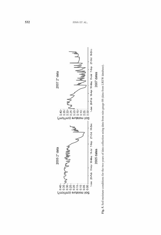
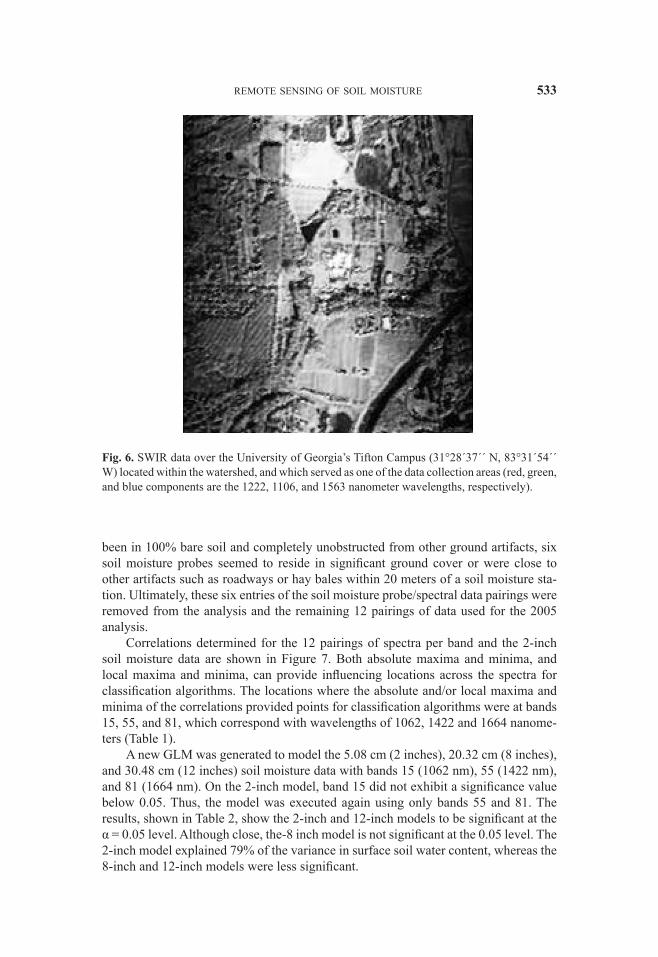
Figure 4 compares the average monthly precipitation for this area with the monthly precipitation for the years of data acquisition, 2005 and 2007. During the months of data acquisition, soil moisture conditions were relatively dry for November 2005 and wet for March 2007 (Fig. 5). Figure 6 shows an example of the data set collected over the University of Georgia Tifton Campus in Tifton, Georgia.

In order to evaluate the utility of the SWIR as a viable tool for soil moisture data collection, the hyperspectral data sets for the two dates were used to establish a General Linear Model (GLM) for each of the three different probe types. In addition, an R2 analysis was used to determine the strength of the linear relationship between the probe and SWIR spectral band data. Recall from the data section that for the 2005 flight each of the 240 spectral sensing lines were binned with their neighbors to enhance the signal measurement. For the 2007 flight four adjacent spectral sensing elements were binned together to further increase the signal measurement.

November 30, 2005

Data from 18 of the soil moisture probes were examined for the November 30, 2005 flight. Many of the soil moisture probes were located in generally bare or unob-structed soil, but some were nestled in significant ground cover, which made it diffi-cult to draw ROIs with confidence. While none of the soil moisture probes may have

Fig. 4. Average monthly precipitation for LREW from 1968 to 2007, with 2005 and 2007 high-lighted (data from LREW database).

532 finn et al.

Fig.

5. S

oil m

oist

ure

cond

ition

s for

the

two

year

s of d

ata

colle

ctio

n us

ing

data

from

rain

gau

ge 0

8 (d

ata

from

LR

EW d

atab

ase)

.


been in 100% bare soil and completely unobstructed from other ground artifacts, six soil moisture probes seemed to reside in significant ground cover or were close to other artifacts such as roadways or hay bales within 20 meters of a soil moisture sta-tion. Ultimately, these six entries of the soil moisture probe/spectral data pairings were removed from the analysis and the remaining 12 pairings of data used for the 2005 analysis.

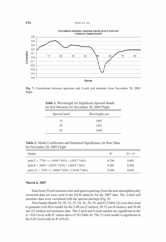
Correlations determined for the 12 pairings of spectra per band and the 2-inch soil moisture data are shown in Figure 7. Both absolute maxima and minima, and local maxima and minima, can provide influencing locations across the spectra for classification algorithms. The locations where the absolute and/or local maxima and minima of the correlations provided points for classification algorithms were at bands 15, 55, and 81, which correspond with wavelengths of 1062, 1422 and 1664 nanome-ters (Table 1).

A new GLM was generated to model the 5.08 cm (2 inches), 20.32 cm (8 inches), and 30.48 cm (12 inches) soil moisture data with bands 15 (1062 nm), 55 (1422 nm), and 81 (1664 nm). On the 2-inch model, band 15 did not exhibit a significance value below 0.05. Thus, the model was executed again using only bands 55 and 81. The results, shown in Table 2, show the 2-inch and 12-inch models to be significant at the α = 0.05 level. Although close, the-8 inch model is not significant at the 0.05 level. The 2-inch model explained 79% of the variance in surface soil water content, whereas the 8-inch and 12-inch models were less significant.

Fig. 6. SWIR data over the University of Georgia’s Tifton Campus (31°28´37´´ N, 83°31´54´´ W) located within the watershed, and which served as one of the data collection areas (red, green, and blue components are the 1222, 1106, and 1563 nanometer wavelengths, respectively).

534 finn et al.

March 6, 2007

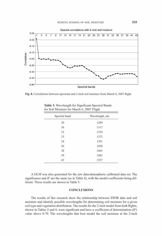
Data from 29 soil moisture sites and spectra pairings from the non- atmospherically corrected data set were used in the GLM analysis for the 2007 data. The 2-inch soil moisture data were correlated with the spectra pairings (Fig. 8).

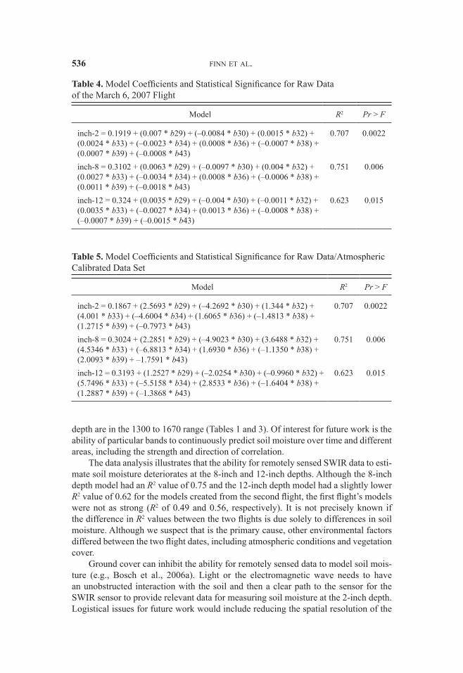
Nine bands (Bands 29, 30, 32, 33, 34, 36, 38, 39, and 43 [Table 3]) were then used to generate a GLM to model for the 5.08 cm (2 inches), 20.32 cm (8 inches), and 30.48 cm (12 inches) soil moisture data. The 2-inch and 8-inch models are significant at the α = 0.01 level with R2 values above 0.70 (Table 4). The 12-inch model is significant at the 0.05 level with an R2 of 0.62.

Fig. 7. Correlations between spectrum and 2-inch soil moisture from November 30, 2005 flight.

Table 1. Wavelength for Significant Spectral Bands for Soil Moisture for November 30, 2005 Flight

Spectral band Wavelength, nm

15 106255 142281 1664

Table 2. Model Coefficients and Statistical Significance for Raw Data for November 30, 2005 Flight

Model R2 Pr > F

inch-2 = .7728 + (–.0399 * b55) + (.0107 * b81) 0.786 0.001inch-8 = .3895 + (.0193 * b55) + (.0055 * b81) 0.485 0.050inch-12 = .7549 + (–.0468 * b55) + (.0148 * b81) 0.560 0.026


A GLM was also generated for the raw data/atmospheric calibrated data set. The significance and R2 are the same (as in Table 4), with the model coefficients being dif-ferent. These results are shown in Table 5.

CONCLUSIONS

The results of this research show the relationship between SWIR data and soil moisture and identify possible wavelengths for determining soil moisture for a given soil type and vegetation distribution. The results for the 2-inch model from both flights, shown in Tables 2 and 4, were significant and have a coefficient of determination (R2) value above 0.70. The wavelengths that best model the soil moisture at the 2-inch

Fig. 8. Correlations between spectrum and 2-inch soil moisture from March 6, 2007 flight.

Table 3. Wavelength for Significant Spectral Bands for Soil Moisture for March 6, 2007 Flight

Spectral band Wavelength, nm

29 129930 131732 135433 137234 139136 142838 146539 148343 1557

536 finn et al.

depth are in the 1300 to 1670 range (Tables 1 and 3). Of interest for future work is the ability of particular bands to continuously predict soil moisture over time and different areas, including the strength and direction of correlation.

The data analysis illustrates that the ability for remotely sensed SWIR data to esti-mate soil moisture deteriorates at the 8-inch and 12-inch depths. Although the 8-inch depth model had an R2 value of 0.75 and the 12-inch depth model had a slightly lower R2 value of 0.62 for the models created from the second flight, the first flight’s models were not as strong (R2 of 0.49 and 0.56, respectively). It is not precisely known if the difference in R2 values between the two flights is due solely to differences in soil moisture. Although we suspect that is the primary cause, other environmental factors differed between the two flight dates, including atmospheric conditions and vegetation cover.

Ground cover can inhibit the ability for remotely sensed data to model soil mois-ture (e.g., Bosch et al., 2006a). Light or the electromagnetic wave needs to have an unobstructed interaction with the soil and then a clear path to the sensor for the SWIR sensor to provide relevant data for measuring soil moisture at the 2-inch depth. Logistical issues for future work would include reducing the spatial resolution of the

Table 4. Model Coefficients and Statistical Significance for Raw Data of the March 6, 2007 Flight

Model R2 Pr > F

inch-2 = 0.1919 + (0.007 * b29) + (–0.0084 * b30) + (0.0015 * b32) + (0.0024 * b33) + (–0.0023 * b34) + (0.0008 * b36) + (–0.0007 * b38) + (0.0007 * b39) + (–0.0008 * b43)

0.707 0.0022

inch-8 = 0.3102 + (0.0063 * b29) + (–0.0097 * b30) + (0.004 * b32) + (0.0027 * b33) + (–0.0034 * b34) + (0.0008 * b36) + (–0.0006 * b38) + (0.0011 * b39) + (–0.0018 * b43)

0.751 0.006

inch-12 = 0.324 + (0.0035 * b29) + (–0.004 * b30) + (–0.0011 * b32) + (0.0035 * b33) + (–0.0027 * b34) + (0.0013 * b36) + (–0.0008 * b38) + (–0.0007 * b39) + (–0.0015 * b43)

0.623 0.015

Table 5. Model Coefficients and Statistical Significance for Raw Data/Atmospheric Calibrated Data Set

Model R2 Pr > F

inch-2 = 0.1867 + (2.5693 * b29) + (–4.2692 * b30) + (1.344 * b32) + (4.001 * b33) + (–4.6004 * b34) + (1.6065 * b36) + (–1.4813 * b38) + (1.2715 * b39) + (–0.7973 * b43)

0.707 0.0022

inch-8 = 0.3024 + (2.2851 * b29) + (–4.9023 * b30) + (3.6488 * b32) + (4.5346 * b33) + (–6.8813 * b34) + (1.6930 * b36) + (–1.1350 * b38) + (2.0093 * b39) + –1.7591 * b43)

0.751 0.006

inch-12 = 0.3193 + (1.2527 * b29) + (–2.0254 * b30) + (–0.9960 * b32) + (5.7496 * b33) + (–5.5158 * b34) + (2.8533 * b36) + (–1.6404 * b38) + (1.2887 * b39) + (–1.3868 * b43)

0.623 0.015


spectral data to minimize interaction with artifacts such as roadways and buildings. In addition, researchers could look more closely at the relationship between reflec-tance and soil moisture where there is ground cover and ascertain the Normalized Difference Vegetation Index (NDVI) in those areas. This could establish a minimum NDVI for ground cover that would allow for estimation of soil moisture. Alternatively, they could establish the vegetative (spectral) response of the ground cover to use as a proxy for soil moisture.

The benefits of hyperspectral data are twofold. First, the spatial resolution (ca. 6 m for this study) is much finer than the datasets used in previous LREW studies by Jackson et al. (2005) and Bosch et al. (2006a) (ca. 3 km for the PSR/CX X-band and 40–75 km for the AMSR-E X-band). In addition, it is worthwhile to note that this higher spatial resolution (by an order of magnitude) is particularly important for investigations of watersheds, where accurate spatial representation can impact water resource decisions. Furthermore, although hyperspectral flights are weather depen-dent, as they are mounted on aircraft and not satellites, researchers have some control over the temporal resolution. Therefore, the inherent characteristics of the hyperspec-tral data directly relate to its strengths in determining soil moisture.

Even though the use of microwave sensors does warrant further research, the goal of this study was to investigate the potential utility of hyperspectral data with SWIR sensors to determine soil moisture. Our results indicate that, at least for a 2-inch depth, hyperspectral sensors can be used to identify soil moisture, most notably in the SWIR range. For situations where satellite-mounted microwave sensors are not an optimal choice, especially in regard to spatial or temporal constraints, aircraft-mounted hyper-spectral sensors can be a valid and useful alternative. Although the sensor used in this study was limited to UV, VNIR, and SWIR, additional future studies using hyperspec-tral sensors with microwave and thermal capabilities are of interest, as this study has shown the potential of hyperspectral data for soil moisture evaluation.

Aside from the microwave data sources mentioned above (PSR/CX and AMSR-E), the Moderate Resolution Imaging Spectroradiometer (MODIS) can be used to derive the temperature/vegetation dryness index (TVDI), which can be used to make infer-ences about soil moisture. The spatial resolution of MODIS is finer than PSR/CX and AMSR-E (between 250 and 1000 m), but it is still coarser than the hyperspectral data used in this study. In addition, the temporal resolution differences (satellite versus air-craft) may also be a determining factor in sensor choice. Although an area of potential future research would be to evaluate the potential of MODIS to determine soil mois-ture in the LREW, it is beyond the scope of this study.

The research described herein provides evidence for the utility of developing SWIR remote sensing analysis to assess soil moisture, particularly for soil moisture measurements at the depth of two inches. The ability to use remote sensing techniques to obtain soil moisture information over a large area could decrease reliance on in situ point measurements, as well as quickly provide data to researchers and agriculturalists. Further studies to test the relationships established in this study and to test their applica-bility to other geographic areas could provide new insights in soil moisture research.

REFERENCES

Barnes, E. M., Sudduth, K. A., Hummel, J. W., Lesch, S. M., Corwin, D. L., Yang, C. H., Daughtry, C. S. T., and W. C. Bausch, 2003, “Remote- and Ground-Based

538 finn et al.

Sensor Techniques to Map Soil Properties,” Photogrammetric Engineering and Remote Sensing, 69(6):619–630.

Baumgardner, M. F., Silva, L. F., Biehl, L. L., and E. R. Stoner, 1985, “The Reflec-tance Properties of Soils,” Advances in Agronomy, 38:1–44.

Bosch, D. D., Lakshmi, V., Jackson, T. J., Choi, M., and J. M. Jacobs, 2006a, “Large Scale Measurements of Soil Moisture for Validation of Remotely Sensed Data: Georgia Soil Moisture Experiment of 2003,” Journal of Hydrology, 323(1–4):120–137.

Bosch, D. D., Sheridan, J. M., and L. K. Marshall, 2007, “Precipitation, Soil Moisture, and Climate Database, Little River Experimental Watershed, Georgia, United States,” Water Resources Research, 43(9).

Bosch, D. D., Sullivan, D. G., and J. M. Sheridan, 2006b, “Hydrologic Impacts of Land-Use Changes in Coastal Plain Watersheds,” Transactions of the ASABE, 49(2):423–432.

Bushnell, T. M., 1932, “A New Technique in Soil Mapping,” American Soil Survey Bulletin, 13:74–81.

Chavez, P. S. and D. J. Mackinnon, 1994, “Automatic Detection of Vegetation Changes in the Southwestern United States Using Remotely Sensed Images,” Photogram-metric Engineering and Remote Sensing, 60(5):571–583.

Crow, W. T., Bindlish, R., and T. J. Jackson, 2005, “The Added Value of Space-borne Passive Microwave Soil Moisture Retrievals for Forecasting Rainfall-Runoff Partitioning,” Geophysical Research Letters, 32(18):L18401 [doi:10.1029/2005GL023543].

Daughtry, C. S. T., Hunt, E. R. J., and P. C. Doraiswamy, 2002, “Assessing Carbon Dynamics in Agriculture Using Remote Sensing,” in International Symposium on Evaluation of Terrestrial Carbon Storage and Dynamics by In-situ and Remote Sensing Measurements, 28–38.

Engman, E. T., 1999, “Remote Sensing in Hydrology,” in Assessment of Non–Point Source Pollution in the Vadose Zone, Corwin, D. L., Loague, K., and T. R. Ellsworth (Eds.), Washington, DC: American Geophysical Union, Geophysical Monograph 108.

Giraldo, M. A., Bosch, D., Madden, M., Usery, L., and C. Kvien, 2008, “Landscape Complexity and Soil Moisture Variation in South Georgia, USA, for Remote Sensing Applications,” Journal of Hydrology, 357(3–4):405–420.

Giraldo, M. A., Madden, M., and D. Bosch, 2009, “Land Use/Land Cover and Soil Type Covariation in a Heterogeneous Landscape for Soil Moisture Studies Using Point Data,” GIScience & Remote Sensing, 46: 77–100.

Gish, T. J., Buss, P., Daughtry, C. S. T., Dulaney, W. P., and C. Walthall, 2002, “Esti-mating Corn Grain Yield from Temporal Variations of Soil Moisture” in Proceed-ings of 6th International Conference on Precision Agriculture and Other Preci-sion Resource Management Conference, Bloomington, MN, 14–17 July 2002.

Grandjean, G., Cerdan, O., Richard, G., Cousin, I., P. L., Tabbagh, B., Van Wesemael, B., Stevens, A., Lambot, S., and F. Carre, 2010, “Digisoil: An Integrated Sys-tem of Data Collection Technologies for Mapping Soil Properties,” in Proximal Soil Sensing, Viscarra Rossel, R. A., McBratney, A., and B. Minasny (Eds.), New York, NY: Springer, 468 p.


Helms, D., Effland, A. B. W., and P. J. Durana, 2002, “Appendix A, Chronology of the U.S. Soil Survey,” in Profiles in the History of the U.S. Soil Survey, Ames, IA: Iowa State University Press.

Jackson, T. J., 2003, “Satellite Microwave Remote Sensing of Soil Moisture: Current and Future Data For Hydrology,” in Fifth International Conference on Electro-magnetic Wave Interaction with Water and Moist Substances, Rotorua, NZ.

Jackson, T. J., Bindlish, R., Gasiewski, A. J., Stankov, B., Klein, M., Njoku, E. G., Bosch, D., Coleman, T., Laymon, C., and P. Starks, 2005, “Polarimetric Scanning Radiometer C and X Band Microwave Observations During SMEX03,” IEEE Transactions on Geoscience and Remote Sensing, 43(11): 2418–2430.

Jackson, T. J., Cosh, M. H., Bindlish, R., Starks, P. J., Bosch, D. D., Seyfried, M., Goodrich, D. C., Moran, M. S., and J. Du, 2010, “Validation of Advanced Microwave Scanning Radiometer Soil Moisture Products,” IEEE Transactions on Geoscience and Remote Sensing, 48(12):4256– 4272.

Jackson, T. J., Oneill, P. E., and C. T. Swift, 1997, “Passive Microwave Observation of Diurnal Surface Soil Moisture,” IEEE Transactions on Geoscience and Remote Sensing, 35(5):1210–1222.

Jensen, J. R. and M. E. Hodgson, 2004, “Remote Sensing of Biophysical Variables and Urban/Suburban Phenomena,” in Geography and Technology, Brunn, S. D., Cutter, S. L., and J. W. Harrington (Eds.), Dordrecht, The Netherlands: Kluwer Academic Publishers, 109–154.

Jensen, J. R., Saalfeld, A., Broome, F., Cowen, D., Price, K., Ramsey, D., Lapine, L., and E. L. Usery, 2005, “Spatial Data Acquisition and Integration,” in A Research Agenda for Geographic Information Science, McMaster, R. B. and E. L. Usery (Eds.), Boca Raton: CRC Press, 416 p.

Katra, I., Blumberg, D. G., Lavee, H., and P. Sarah, 2006, “A Method for Estimating the Spatial Distribution of Soil Moisture of Arid Microenvironments by Close Range Thermal Infrared Imaging,” International Journal of Remote Sensing, 27(12):2599–2611.

Lewis, D. and M. P. Finn, 2007, “Soil Moisture Estimation Using Hyperspectral SWIR Imagery,” in The American Geophysical Union Annual Meeting, San Francisco, CA, 10–14 December 2007.

Lobell, D. B. and G. P. Asner, 2002, “Moisture Effects on Soil Reflectance,” Soil Science Society of America Journal, 66(3):722–727.

McCabe, M. and E. Wood, 2006, “Scale Influences on the Remote Estimation of Evapotranspiration Using Multiple Satellite Sensors,” Remote Sensing of Envi-ronment, 105(4):271–285.

Milfred, C. J. and R. W. Kiefer, 1976, “Analysis of Soil Variability with Repetitive Aerial Photography,” Soil Science Society of America Journal, 40(4):553–557.

Mira, M., Valor, E., Caselles, V., Rubio, E., Coll, C., Niclos, R., Sanchez, J. M., and R. Boluda, 2010, “Soil Moisture Effect on Thermal Infrared (8–13 μm) Emissivity,” IEEE Transactions on Geoscience and Remote Sensing, 48(5):2251–2260.

Moran, M. S., Vidal, A., Troufleau, D., Inoue, Y., and T. A. Mitchell, 1998, “Ku- and C-Band SAR for Discriminating Agricultural Crop and Soil Conditions,” IEEE Transactions on Geoscience and Remote Sensing, 36(1):265–272.

540 finn et al.

Mouazen, A. M., Karoui, R., De Baerdemaeker, J., and H. Ramon, 2006, “Character-ization of Soil Water Content Using Measured Visible and Near Infrared Spectra,” Soil Science Society of America Journal, 70(4):1295–1302.

Njoku, E. G., and D. Entekhabi, 1996, “Passive Microwave Remote Sensing of Soil Moisture,” Journal of Hydrology, 184(1–2):101–129.

NOAA (National Atmospheric and Atmospheric Administration), 2002, Climatog-raphy of the United States, No. 81: Monthly Station Normals of Temperature, Precipitation, and Heating and Cooling Degree Days, 1971–2000. Asheville, NC: National Climatic Data Center.

Press, W. H., Teukolsky, S. A., Vetterling, W. T., and B. P. Flannery, 1997, Numeri-cal Recipes in C: The Art of Scientific Computing. Cambridge, UK, Cambridge University Press.

Price, J. C., 1987, “Calibration of Satellite Radiometers and the Comparison of Veg-etation Indices,” Remote Sensing of Environment, 21(1):15–27.

Priest, S., 2004, Evaluation of Ground-Water Contribution to Streamflow in Coastal Georgia and Adjacent Parts of Florida and South Carolina,” Reston, VA: U. S. Geological Survey, Scientific Investigations Report 2004-5265.

Sahoo, A. K., Houser, P. R., Ferguson, C., Wood, E. F., Dirmeyer, P. A., and M. Kafatos, 2008, “Evaluation of AMSR-E Soil Moisture Results Using the In-situ Data Over the Little River Experimental Watershed, Georgia,” Remote Sensing of Environ-ment, 112(6):3142–3152.

Salvucci, G. D., Saleem, J. A., and R. Kaufmann, 2002, “Investigating Soil Moisture Feedbacks on Precipitation with Tests of Granger Causality,” Advances in Water Resources, 25:1305–1312.

Slaughter, D. C., Pelletier, M. G., and S. K. Upadhyaya, 2001, “Sensing Soil Moisture Using NIR Spectroscopy,” Applied Engineering in Agriculture, 17(2):241–247.

Steele-Dunne, S. C., Rutten, M. M., Krzeminska, D. M., Hausner, M., Tyler, S. W., Selker, J., Bogaard, T. A., and N. C. V. de Giesen, 2010, “Feasibility of Soil Mois-ture Estimation Using Passive Distributed Temperature Sensing,” Water Resourc-es Research, 46:W03534.

Vogt, F., Banerji, S., and K. Booksh, 2004, “Utilizing Three-Dimensional Wavelet Transforms for Accelerated Evaluation of Hyperspectral Image Cubes,” Journal of Chemometrics, 18(7–8):350–362.

Walthall, C. L., Kaul, M., Timlin, D. J., and C. S. T. Daughtry, 2001, “Linking Within-Field Crop Response with Soil Characteristics to Define Crop Response Zones for Management Zone Delineation,” in Proceedings of the 3rd International Con-ference Geospatial Information in Agriculture and Forestry, Denver, CO, 5–7 November 2001.

Warren, J. W., Peacock, K., Darlington, E., Murchie, S. L., Oden, S. F., Hayes, J. R., Bell, J. F., Krein, S. J., and A. Mastandrea, 1997, “Near Infrared Spectrometer for the near Earth Asteroid Rendezvous Mission,” Space Science Reviews, 82(1–2):101–167.

Whiting, M. L., Li, L., and S. L. Ustin, 2004, “Predicting Water Content Using Gauss-ian Model on Soil Spectra,” Remote Sensing of Environment, 89(4):535–552.

Ulaby, F. T., Moore, R. K., and A. K. Fung, 1986, Microwave Remote Sensing: Active and Passive, Vol. III, from Theory to Application, Dedham, MA: Artech House.

remote sensing of soil moisture using airborne ... sensing of soil moisture using airborne...

Documents