rendezvous and close proximity operations for an
TRANSCRIPT

Rendezvous and Close Proximity Operations for
an Interplanetary CubeSat around Small Bodies
Boumchita Wail ID: 899587
Department of Aerospace Science and Technology (DAER)
Politecnico di Milano
Supervisor
Prof. Topputo FrancescoFranzese Vittorio
Giordano Carmine
Master of Science in Space Engineering
April 29, 2020


At some point, everything’s gonna go south on you... everything’s
going to go south and you’re going to say, this is it. This is how I
end. Now you can either accept that, or you can get to work.
That’s all it is. You just begin. You do the math.
You solve one problem... and you solve the next one... and then the
next.
And If you solve enough problems, you get to come home.
Ringraziamenti
Bismillah.
Questo lavoro di tesi rappresenta la conclusione di un percorso du-
rato anni, che non sarebbe stato possibile se non grazie all’aiuto e alla
pazienza di molte persone che vorrei ringraziare.
Il primo ringraziamento va al Professor Francesco Topputo che mi ha
dato la possibilita di approfondire e sviluppare un argomento affasci-
nante e interessante come quello del design di un segmento di una
missione spaziale. Ringrazio Carmine Giordano e Vittorio Franzese
che fin dall’inizio mi hanno seguito, dandomi la loro disponibilita e
trasmettendomi le loro conoscenze, necessarie per riuscire a entrare
meglio nell’ottica del lavoro.
Il percorso universitario non poteva essere lo stesso senza la compag-
nia delle persone con cui ho passato la maggior parte del tempo.
Vorrei ringraziare la mia seconda famiglia che ho avuto la fortuna di
incontrare casualmente il primo giorno che mi son trasferito a Mi-
lano in quel pianerottolo in Via Giovanni Battista Vare. Un grazie
particolare a Stefano e Andrea per avermi motivato quando ero giu,
incoraggiato quando non ce la facevo piu e aiutato quando ne avevo
piu bisogno. Ricordero sempre i lunghi pomeriggi e le notti di studio,
le pile di Monster e Red Bull che si accumulavano inesorabilmente
sulle nostre scrivanie, le gioie e le delusioni che ci hanno accompa-
gnato a seguito di un esame o di un progetto e, infine, i pomeriggi
spensierati ai parchi dopo una sessione a godersi un gelato e a far
finta di saper giocare a pallavolo. Riuscire a ottenere questa laurea
tanto ambita e stata dura, ma con colleghi e amici come voi al mio
fianco e stato quasi divertente.
Vorrei ringraziare inoltre tutte le amicizie nate a Milano, soprattutto
nell’ultimo periodo, facendomi riscoprire quello spirito e senso di ap-
partenenza arabo che non avevo mai approfondito prima. Fratelli e
sorelle che si preoccupano per me anche a distanza, nonostante io non
sia riuscito a dedicar loro il tempo che meritavano. A loro va tutta la
mia stima e il mio affetto.
Infine, un ringraziamento alla mia famiglia. Hamid e Houriya, i due
genitori che ogni figlio dovrebbe avere. Capaci di credere in me anche
nei momenti in cui avevo perso la fiducia in me stesso, ad un passo
dal mollare tutto in quanto non mi ritenevo adatto a quella facolta
che, inshAllah, mi avrebbe permesso di raggiungere obiettivi che fin
da bambino osavo solo sognare. Ancora non capisco appieno con che
coraggio abbiano deciso di accompagnarmi in questa avventura. Yas-
mine, Zakaria e Karim, i miei fratelli da cui mi son allontanato per
6 anni per inseguire questo sogno. Perdonatemi per non avervi ded-
icato abbastanza tempo e vi ringrazio per avermi fatto compagnia,
soprattutto in quest’ultimo periodo.
Alhamdulillah per tutto quanto.
Abstract
In recent years, missions to celestial bodies have been carried out.
However, these missions were expensive and were directed towards
large asteroids or comets. This work will focus on the design of a
mission directed towards a small body using an interplanetary Cube-
Sat, defining all the needed operations to characterize the small body.
This statement introduces two limitations with respect to the previ-
ous mission: to use a cheaper vehicle and to target a celestial body
whose gravitational attraction will not affect the spacecraft dynamics.
Interest in this topic stems from the fact that literature is poor in in-
formation on this type of asteroids and the fact that these bodies can
be a useful resource in the future. The design of the trajectories was
carried out after developing a dynamic model and, subsequently, de-
veloping a program that allows to make the design of the trajectory by
changing each time certain parameters. In addition, the performance
of Vision-based Navigation is discussed. To perform this analysis, a
3D modeling program was used to faithfully simulate the asteroid ap-
proach. The analysis of navigation based on the Center of Brightness
have shown how, taking into account some factors, it is possible to
obtain a good level of navigation.
Sommario
Negli ultimi anni sono state progettate varie missioni verso i corpi
celesti. Tuttavia, queste missioni erano costose ed erano dirette verso
asteroidi o comete di grandi dimensioni. Questo lavoro si concen-
trera sulla progettazione di una missione diretta verso un asteroide di
piccole dimensioni usando un CubeSat interplanetario, identificando
tutte le operazioni necessarie per caratterizzare il corpo celeste. Ven-
gono introdotti due limiti rispetto alle missioni precedenti: l’utilizzo
di un veicolo piu economico e il puntare verso un corpo celeste la
cui attrazione gravitazionale sara troppo debole per influenzare la di-
namica del veicolo spaziale. L’interesse per questo argomento nasce
dal fatto che la letteratura e povera di informazioni su questo tipo di
asteroidi e dal fatto che questi corpi potranno essere utili risorse in fu-
turo. La progettazione delle traiettorie e stata effettuata sviluppando
un adeguato modello dinamico e, successivamente, creando un soft-
ware che consente di progettare la traiettoria del veicolo cambiando
di volta in volta determinati parametri. Inoltre, vengono discusse le
prestazioni della Navigazione basata sulle immagini acquisite dalla
camera a bordo del veicolo spaziale. Per eseguire questa analisi, e
stato utilizzato un programma di modellazione 3D per simulare fedel-
mente l’approccio all’asteroide. L’analisi della navigazione basata sul
Centro di Luminosita ha mostrato come, tenendo conto di alcune fat-
tori, sia possibile ottenere un buon livello di navigazione.

Contents
1 Introduction 1
1.1 Motivations . . . . . . . . . . . . . . . . . . . . . . . . . . . . . . 1
1.2 Objectives and Contributions . . . . . . . . . . . . . . . . . . . . 3
1.3 Overview of the Thesis . . . . . . . . . . . . . . . . . . . . . . . . 4
2 State of the Art 6
2.1 Hayabusa . . . . . . . . . . . . . . . . . . . . . . . . . . . . . . . 7
2.1.1 Approach Phase and Target Detection . . . . . . . . . . . 8
2.1.2 Initial Characterization Phase . . . . . . . . . . . . . . . . 9
2.1.3 Global Mapping Phase . . . . . . . . . . . . . . . . . . . . 10
2.1.4 AOCS and GNC System . . . . . . . . . . . . . . . . . . . 11
2.1.5 Shape and Surface Topography Modeling . . . . . . . . . . 12
2.2 Rosetta . . . . . . . . . . . . . . . . . . . . . . . . . . . . . . . . 14
2.2.1 Approach Phase . . . . . . . . . . . . . . . . . . . . . . . . 14
2.2.2 Initial Characterization Phase . . . . . . . . . . . . . . . . 15
2.2.3 Global Mapping Phase . . . . . . . . . . . . . . . . . . . . 16
2.2.4 Shape Modeling . . . . . . . . . . . . . . . . . . . . . . . . 17
3 System’s Architecture and Dynamic Models 19
3.1 Imaging System . . . . . . . . . . . . . . . . . . . . . . . . . . . . 20
vi
CONTENTS
3.2 Asteroids . . . . . . . . . . . . . . . . . . . . . . . . . . . . . . . 23
3.3 SPICE Toolkit . . . . . . . . . . . . . . . . . . . . . . . . . . . . 27
3.4 Dynamic models . . . . . . . . . . . . . . . . . . . . . . . . . . . 27
3.4.1 Free-motion dynamic equation . . . . . . . . . . . . . . . . 27
3.4.2 Complete equation of motion . . . . . . . . . . . . . . . . 29
3.4.3 Thrust and Isp model . . . . . . . . . . . . . . . . . . . . . 30
3.5 CPO Calculator . . . . . . . . . . . . . . . . . . . . . . . . . . . . 31
3.6 Vision-based Navigation Algorithm . . . . . . . . . . . . . . . . . 35
4 Mission Design 37
4.1 Absolute Navigation Phase . . . . . . . . . . . . . . . . . . . . . . 41
4.1.1 Target Detection and Identification . . . . . . . . . . . . . 41
4.1.2 Navigation . . . . . . . . . . . . . . . . . . . . . . . . . . . 44
4.1.3 Lightcurve analysis . . . . . . . . . . . . . . . . . . . . . . 46
4.1.4 Summary . . . . . . . . . . . . . . . . . . . . . . . . . . . 47
4.2 Relative Navigation Phase - Part 1 . . . . . . . . . . . . . . . . . 48
4.2.1 Relative distance estimation . . . . . . . . . . . . . . . . . 48
4.2.2 Navigation . . . . . . . . . . . . . . . . . . . . . . . . . . . 49
4.2.3 Debris Analysis . . . . . . . . . . . . . . . . . . . . . . . . 51
4.2.4 Summary . . . . . . . . . . . . . . . . . . . . . . . . . . . 51
4.3 Relative Navigation Phase - Part 2 . . . . . . . . . . . . . . . . . 52
4.3.1 Navigation . . . . . . . . . . . . . . . . . . . . . . . . . . . 53
4.3.2 Summary . . . . . . . . . . . . . . . . . . . . . . . . . . . 56
4.4 Close Proximity Operations . . . . . . . . . . . . . . . . . . . . . 57
4.4.1 CPO Trajectory design . . . . . . . . . . . . . . . . . . . . 58
4.4.1.1 Spacecraft: M-ARGO . . . . . . . . . . . . . . . 60
4.4.2 Guidance . . . . . . . . . . . . . . . . . . . . . . . . . . . 61
4.4.2.1 Nominal case . . . . . . . . . . . . . . . . . . . . 62
vii
CONTENTS
4.4.2.2 High visibility case . . . . . . . . . . . . . . . . . 63
4.4.2.3 Maximum phase angle case . . . . . . . . . . . . 66
4.4.2.4 Shape analysis . . . . . . . . . . . . . . . . . . . 67
4.4.3 Navigation . . . . . . . . . . . . . . . . . . . . . . . . . . . 68
4.4.4 Geophysical properties determination . . . . . . . . . . . . 73
4.4.5 Dynamic state determination . . . . . . . . . . . . . . . . 74
4.4.6 Summary . . . . . . . . . . . . . . . . . . . . . . . . . . . 75
4.5 Disposal strategy: Landing . . . . . . . . . . . . . . . . . . . . . . 76
4.6 Error Sources . . . . . . . . . . . . . . . . . . . . . . . . . . . . . 77
5 Severity and Likelihood Categorization 78
5.1 Risk Matrix . . . . . . . . . . . . . . . . . . . . . . . . . . . . . . 79
5.1.1 Reaction Wheel failure . . . . . . . . . . . . . . . . . . . . 80
5.1.2 IMU failure . . . . . . . . . . . . . . . . . . . . . . . . . . 80
5.1.3 Laser Altimeter failure . . . . . . . . . . . . . . . . . . . . 81
6 Conclusions 82
References 88
viii
List of Figures
2.1 Approach Phase OD (1σ uncertainties) . . . . . . . . . . . . . . . 8
2.2 On board navigation system data flow diagram . . . . . . . . . . 9
2.3 The Z position history . . . . . . . . . . . . . . . . . . . . . . . . 11
2.4 Block Diagram of AOCS/GNC System . . . . . . . . . . . . . . . 11
2.5 a) Schematic representation of the scenario. b) 3D model construc-
tion procedure . . . . . . . . . . . . . . . . . . . . . . . . . . . . . 13
2.6 Effect of impact vector on navigation accuracy . . . . . . . . . . . 15
2.7 Comparison of minimum velocity during 1-leg and 2-leg manoeuvres 16
2.8 Silhouette Carving Method . . . . . . . . . . . . . . . . . . . . . . 17
3.1 Cubesat overall structure . . . . . . . . . . . . . . . . . . . . . . . 20
3.2 Performance comparison between visible and IR cameras . . . . . 22
3.3 General Density-Mass plot for asteroids . . . . . . . . . . . . . . . 24
3.4 General Macroporosity-Mass plot for asteroids . . . . . . . . . . . 25
3.5 3D model of the reference asteroid . . . . . . . . . . . . . . . . . . 25
3.6 3D model of the Rosetta comet . . . . . . . . . . . . . . . . . . . 26
3.7 3D model of the Itokawa asteroid . . . . . . . . . . . . . . . . . . 26
3.8 CPO Calculator software screenshot . . . . . . . . . . . . . . . . . 33
3.9 Scheme of the test of the Navigation algorithm . . . . . . . . . . . 35
3.10 Computation of the CoB . . . . . . . . . . . . . . . . . . . . . . . 36
ix
LIST OF FIGURES
4.1 Mission Overview . . . . . . . . . . . . . . . . . . . . . . . . . . . 38
4.2 Initial distance asteroid detectability domain using NavCam . . . 39
4.3 Initial distance asteroid detectability domain using the Star Tracker 40
4.4 GNC workflow chart . . . . . . . . . . . . . . . . . . . . . . . . . 40
4.5 Schematic representation of the Target detection procedure . . . . 42
4.6 Subtraction method for asteroid identification . . . . . . . . . . . 43
4.7 Reference asteroid against background stars . . . . . . . . . . . . 44
4.8 EKF input/output . . . . . . . . . . . . . . . . . . . . . . . . . . 44
4.9 Vision-based algorithm for attitude change detection . . . . . . . 45
4.10 Stein’s light curve . . . . . . . . . . . . . . . . . . . . . . . . . . . 46
4.11 Asteroid image at the beginning of RelNav Phase Pt.1 . . . . . . 48
4.12 GNC workflow for Relative Navigation Pt.1 . . . . . . . . . . . . 49
4.13 Asteroid recognition algorithm . . . . . . . . . . . . . . . . . . . . 50
4.14 Asteroid model at 5km and at 1km . . . . . . . . . . . . . . . . . 53
4.15 GNC workflow for the second part of Relative Navigation . . . . . 54
4.16 Pixel error as the spacecraft approaches the asteroid . . . . . . . . 54
4.17 67P/CG maximum error case during RelNav pt.2 . . . . . . . . . 55
4.18 CoB on the image plane during the approach to the reference asteroid 55
4.19 CoB on the image plane during the approach to Itokawa . . . . . 56
4.20 CoB on the image plane during the approach to 67P/CG . . . . . 56
4.21 3D hyperspectral model workflow . . . . . . . . . . . . . . . . . . 58
4.22 Trajectory design proposed in the M-ARGO CDF study . . . . . 60
4.23 Vertices enumeration . . . . . . . . . . . . . . . . . . . . . . . . . 60
4.24 Planet and 2000SG344 position at the beginning of CPO . . . . . 61
4.25 CPO trajectory simulation considering CDF parameters . . . . . 62
4.26 CPO trajectory simulation considering the new data from MDR . 63
4.27 Asteroid model at 800m and 400m . . . . . . . . . . . . . . . . . 64
x
LIST OF FIGURES
4.28 Closer CPO trajectory simulation . . . . . . . . . . . . . . . . . . 65
4.29 CPO trajectory simulation keeping the distance from drastical
changes . . . . . . . . . . . . . . . . . . . . . . . . . . . . . . . . 65
4.30 Proposed CPO trajectory solution maximizing the maximum phase
angle . . . . . . . . . . . . . . . . . . . . . . . . . . . . . . . . . . 66
4.31 Different CPO trajectory shapes considered in the parametric study 67
4.32 Pixel error during CPO . . . . . . . . . . . . . . . . . . . . . . . . 69
4.33 67P/CG maximum error case during CPO . . . . . . . . . . . . . 69
4.34 Representation of the logic to determine the initial distance for CPO 71
4.35 Representation of the logic to determine the initial distance for CPO 72
4.36 Representation of the logic to determine the initial distance for CPO 72
4.37 Result of the SWIR hyperspectral analysis capable of identifying
an element with different spectral composition on its surface . . . 73
4.38 EKF SLAM workflow . . . . . . . . . . . . . . . . . . . . . . . . . 74
xi
List of Tables
3.1 Estimated mass and dimension for the candidate asteroids . . . . 23
4.1 Optical instruments specifics . . . . . . . . . . . . . . . . . . . . . 38
4.2 Detection distances by each instrument . . . . . . . . . . . . . . . 38
4.3 M-ARGO mission distance milestones . . . . . . . . . . . . . . . . 39
4.4 List of known and unknown properties of the asteroid at the be-
ginning of the mission . . . . . . . . . . . . . . . . . . . . . . . . 41
4.5 List of known and unknown properties of the asteroid at the end
of AbsNav . . . . . . . . . . . . . . . . . . . . . . . . . . . . . . . 47
4.6 List of known and unknown properties of the asteroid at the end
of RelNav Pt.1 . . . . . . . . . . . . . . . . . . . . . . . . . . . . 52
4.7 List of known and unknown properties of the asteroid at the end
on RelNav Pt.2 . . . . . . . . . . . . . . . . . . . . . . . . . . . . 57
4.8 Quantitative comparison of the different trajectory shapes . . . . 68
4.9 List of known and unknown properties of the asteroid at the end
on CPO . . . . . . . . . . . . . . . . . . . . . . . . . . . . . . . . 76
5.1 Risk analysis matrix . . . . . . . . . . . . . . . . . . . . . . . . . 79
xii

Chapter 1
Introduction
1.1 Motivations
Hayabusa, Rosetta and OSIRIS-REx are just a few missions whose goal was to
visit a celestial body, be it an asteroid or a comet. The foundations on which this
thesis was built are based on the teachings from previous large class missions. In
particular, for the Hayabusa mission the references written by J. Kawaguchi et
al. were essential, in particular ref. [1], [2] and [3] are suggested if the reader
is interested in the details of the mission or in the methods with which the 3D
model of the asteroid was created. Analogously for the Rosetta mission ref. [4],
[5] and [6] were vital.
The aim of this thesis is to define a series of operations that a CubeSat will have
to carry out in order to approach an asteroid and complete all the necessary
Close Proximity Operations (CPO). All as independently as possible. The use of
a CubeSat is dictated by the need to lower the costs of the mission. In fact, the
previous missions were characterized by high costs: Hayabusa cost 150 million
euros [7], OSIRIS-REx cost 800 million euros [8], while Rosetta cost 1.3 billion
1
1.1 Motivations
euros [9]. To make space more accessible even to private companies, the total
cost must be lowered. This can be achieved by using spacecraft which can be
mass-produced instead of building ad-hoc spacecraft each time.
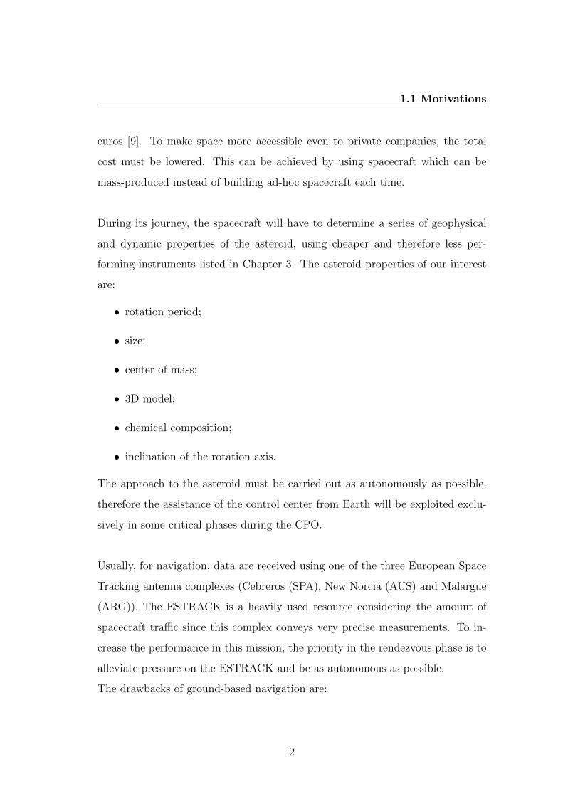
During its journey, the spacecraft will have to determine a series of geophysical
and dynamic properties of the asteroid, using cheaper and therefore less per-
forming instruments listed in Chapter 3. The asteroid properties of our interest
are:
• rotation period;
• size;
• center of mass;
• 3D model;
• chemical composition;
• inclination of the rotation axis.
The approach to the asteroid must be carried out as autonomously as possible,
therefore the assistance of the control center from Earth will be exploited exclu-
sively in some critical phases during the CPO.
Usually, for navigation, data are received using one of the three European Space
Tracking antenna complexes (Cebreros (SPA), New Norcia (AUS) and Malargue
(ARG)). The ESTRACK is a heavily used resource considering the amount of
spacecraft traffic since this complex conveys very precise measurements. To in-
crease the performance in this mission, the priority in the rendezvous phase is to
alleviate pressure on the ESTRACK and be as autonomous as possible.
The drawbacks of ground-based navigation are:
2
1.2 Objectives and Contributions
• Long round-trip time, from many minutes to many hours, depending on the
spacecraft’s position in the Solar System;
• Time to process the data. Orbit determination and maneuver calculation,
convene meetings to make and implement decisions and generate a sequence
of commands and uplink them to spacecraft;
• The lag time between the last navigation update and implementing ma-
neuvers can take from 8 hours to one week losing some science in pointing
instruments.
Incorporating an onboard autonomous navigation system can result in advanta-
geous for many reasons:
• it eliminates the delays due to the round-trip light time;
• it eliminates human factors in ground-based processing;
• it reacts with the latest navigation information.
To guarantee the navigation only optical measurements will be used to get self-
contained data.
1.2 Objectives and Contributions
The main objective of this thesis is to define the Concept of Operations (ConOps)
of an interplanetary mission performed with Cubesats, in particular for the ren-
dezvous and CPO segments.
In defining these operations, problems began to emerge due to the limited tools
on board the spacecraft compared to previous missions. All this was done in order
to reduce the costs of the mission. Other actions have been taken to maximize
the objective:
3
1.3 Overview of the Thesis
• the radiometric support from Earth is limited to some CPO activities;
• no chemical propulsion system was present.
The main propulsion systems are the Electric Propulsion System (EPS) and the
Reaction Control System (RCS). The use of the latter was limited as much as
possible where precise control of the spacecraft had to be obtained. Instead, to
control the attitude, the CubeSat was equipped with a system consisting of three
Reaction Wheels (RW).
In addition to defining these operations, the navigation based on the Center of
Brightness (CoB) and how the spacecraft would perform instead of considering
the Center of Mass (CoM) will also be analyzed. With the results obtained from
the simulations, a solution will be proposed to counter the worsening of naviga-
tion performance. Furthermore, the dynamics of the spacecraft in these segments
will be analyzed and the trajectory design will be made, taking into consideration
that a small body is by definition a celestial body so small as to have a negligible
gravitational field.
Finally, the results will be applied to the M-ARGO mission, the first-ever mission
to rendezvous with an asteroid using Cubesats.
1.3 Overview of the Thesis
The development of the thesis was based on the experiences of the previous
missions. so, after a brief introduction, Chapter 2 will begin by analyzing the
Hayabusa and Rosetta missions. The OSIRIS-REx mission was analyzed and
considered during the development of the thesis, but being a mission still opera-
tional, therefore possibly subject to modifications, it was chosen to not include it
4
1.3 Overview of the Thesis
in the State of Art and to give priority to the two completed missions. Chapter 3
contains a description of the CubeSat of the M-ARGO mission, the instruments
with which it will be equipped, a list of candidate asteroids as possible objectives
of the mission, the dynamic model, a description of the simulation program for
the design of the trajectories and the one used for simulating navigation perfor-
mance. Chapter 4 begins by presenting a general concept of the Rendezvous and
CPO (R&CPO) phases. Then, each segment will be analyzed from an operational
point of view, as well as the design of the trajectory and the analysis of navigation
performance. Finally a disposal strategy will be discussed. In Chapter 5 a risk
analysis will be carried out and an attempt will be made to identify what are the
crucial instruments for the success of the mission.
5
Chapter 2
State of the Art
Summary
The analysis of the State of Art concerning the missions that in the past have
reached a celestial body will be carried out focusing mainly on two missions of
two different space agencies, the Hayabusa mission from JAXA and Rosetta from
ESA.
The reasons why these two missions were chosen are:
• these two missions have reached the smallest celestial bodies that humanity
has achieved, therefore more similar to the subject of this thesis;
• the missions were designed by two different space agencies. It will therefore
be possible to note the different philosophies with which the two missions
were organized;
• both missions are completed, so the literature is full of articles about them.
The analysis of the missions will start from the first detection of the celestial
body until the spacecraft has mapped the target.
6
2.1 Hayabusa
The missions can be divided in the following phases:
• Approach Phase, after detecting the comet with onboard optical sensors,
the spacecraft has to reduce its relative position and velocity and bend its
trajectory towards the celestial body;
• Initial Characterization Phase, in which the main tasks are to identify first
landmarks on the celestial body surface, to determine its shape and rota-
tional state and to obtain an initial estimate of its gravitational field;
• Global Mapping Phase, in which the spacecraft has to map at least 80% of
the body surface and improve the estimate of the navigation parameters.
In the next sections the ConOps of the previously mentioned missions are pre-
sented.
2.1 Hayabusa
Hayabusa is a mission developed by JAXA to reach the asteroid 25143 Itokawa
and, for the first time, take samples from its surface and bring them to Earth.
The mission began in 2003, reached the S-type asteroid in 2005, began its return
in 2007 and landed on Earth in 2010 along with the samples taken.
Various goals have been achieved with this mission, in particular:
• first spacecraft that landed for sampling extra-terrestrial material;
• first spacecraft to land on the surface of the celestial body and lift off again;
• the guidance was obtained with an accuracy of 10−3 m/s;
• first spacecraft to perform cruise via Ion Engines as primary propulsion;
• first spacecraft to demonstrate the possibility of Autonomous Navigation
and Guidance using Optical measurements.
7
2.1 Hayabusa
2.1.1 Approach Phase and Target Detection
The approach phase begins when the asteroid has been identified thanks to the
onboard cameras. Several images were taken and sent to Earth for identifica-
tion, as it is not possible to distinguish the asteroid from the background stars
with a single image. Therefore, these images were taken and compared with the
predicted trajectory ensuring the scientists of the correct identification of the as-
teroid.
A combined use of optical navigation techniques and radiometric information
from Earth has been used to guide Hayabusa to Itokawa. The use of radiomet-
ric information alone would have required a huge amount of data without any
guarantee of the accuracy that would have been obtained. The strategy adopted
consists in providing the information of the spacecraft with respect to Earth us-
ing radiometry, while the determination of the state of the spacecraft relative to
the asteroid was obtained through optical navigation techniques. Therefore this
hybrid strategy has been called Hybrid OPNAV. The measurements obtained
through this technique are less ambiguous and determine the state of the space-
craft in a simpler way.
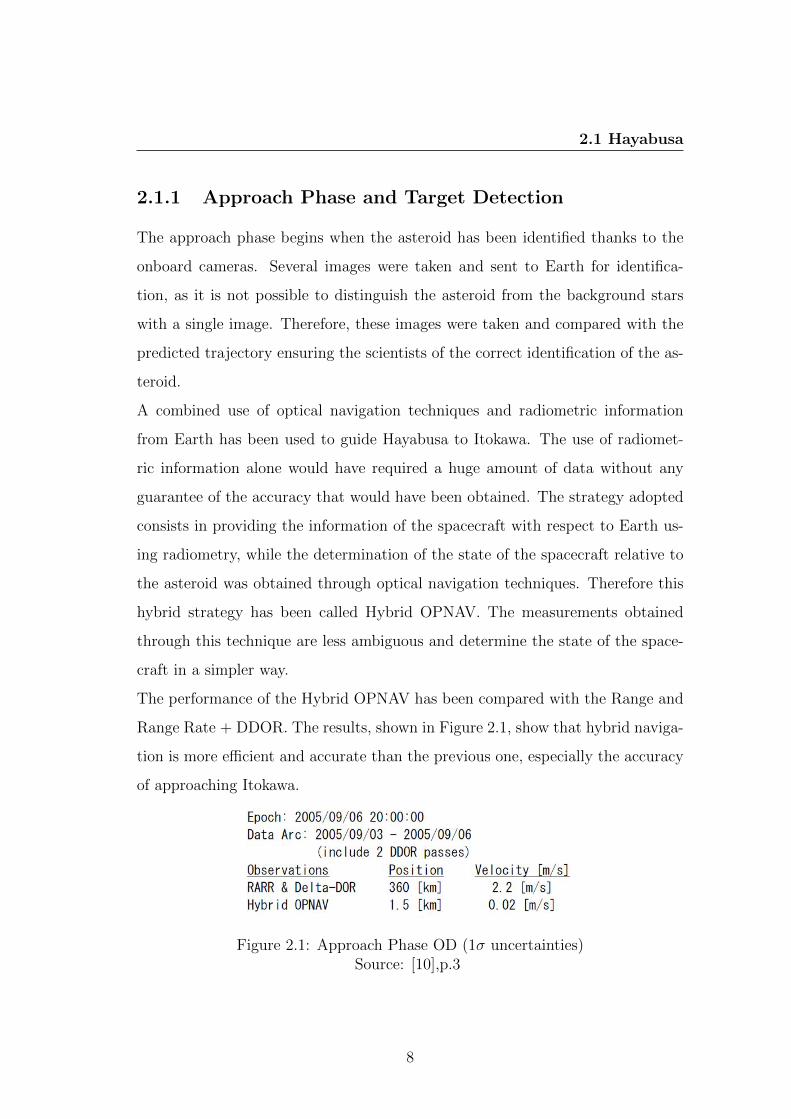
The performance of the Hybrid OPNAV has been compared with the Range and
Range Rate + DDOR. The results, shown in Figure 2.1, show that hybrid naviga-
tion is more efficient and accurate than the previous one, especially the accuracy
of approaching Itokawa.
Figure 2.1: Approach Phase OD (1σ uncertainties)Source: [10],p.3
8
2.1 Hayabusa
Finally, using the acquired images, the Onboard computer (OBC) analyzes the
lightcurve to ensure the correct identification of the objective and to refine the
ground measurements on the rotation period of the asteroid [11]. From the ob-
servations from Earth, the rotation period of the asteroid was estimated to be
12.13± 0.02 hours. The analysis of the lightcurve finally confirmed this value by
measuring a rotation period of 12.132 hours [12].
2.1.2 Initial Characterization Phase
This phase begins 20 km from the asteroid, a location nominated by convention
as a Gate Location by the Japanese space agency. The aim at this point is to
accurately estimate the perturbations due to SRP and begin building a 3D model
of the body.
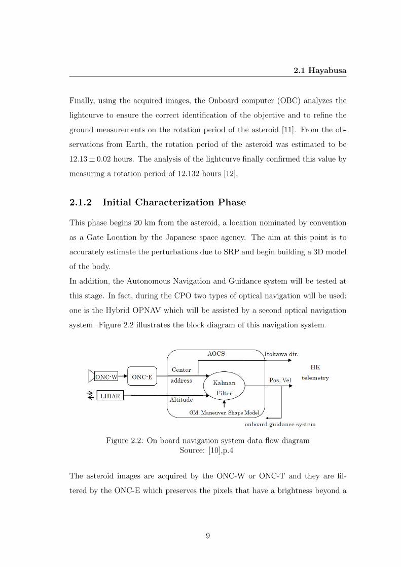
In addition, the Autonomous Navigation and Guidance system will be tested at
this stage. In fact, during the CPO two types of optical navigation will be used:
one is the Hybrid OPNAV which will be assisted by a second optical navigation
system. Figure 2.2 illustrates the block diagram of this navigation system.
Figure 2.2: On board navigation system data flow diagramSource: [10],p.4
The asteroid images are acquired by the ONC-W or ONC-T and they are fil-
tered by the ONC-E which preserves the pixels that have a brightness beyond a
9
2.1 Hayabusa
certain value, it calculates the center of each group of pixels and considers only
the group with most number of illuminated pixels for navigation. Also, LIDAR
provides information regarding the relative distance. The onboard navigation
system acquires data every second and processes the linearized state dynamics
and observation equations in the Kalman filter algorithm.
2.1.3 Global Mapping Phase
This phase begins 7 km from Itokawa, a position named by convention as Home
Position, there will be a detailed observation of the asteroid to determine its
properties and build a detailed 3D model of the asteroid.
At this point the asteroid is close enough to make gravitational force become the
predominant force acting on the spacecraft compared to all other forces, therefore
a precise estimate of this will be made.
During this phase one of the three RWs no longer responds to commands. There-
fore navigation switches to the Dual Reaction Wheel (DRW) mode with a series
of limitations in the frequency and amplitude of the maneuvers necessary for nav-
igation. Not much later, the second RW was unexpectedly malfunctioning and no
longer able to guarantee attitude control. As a result, the GNC switched to RCS
[13]. With the use of the RCS together with considerations on the architecture
and positioning of the thrusters, the attitude has been stabilized. Although the
pointing error in RCS mode was greater than that in DRW mode, hovering of
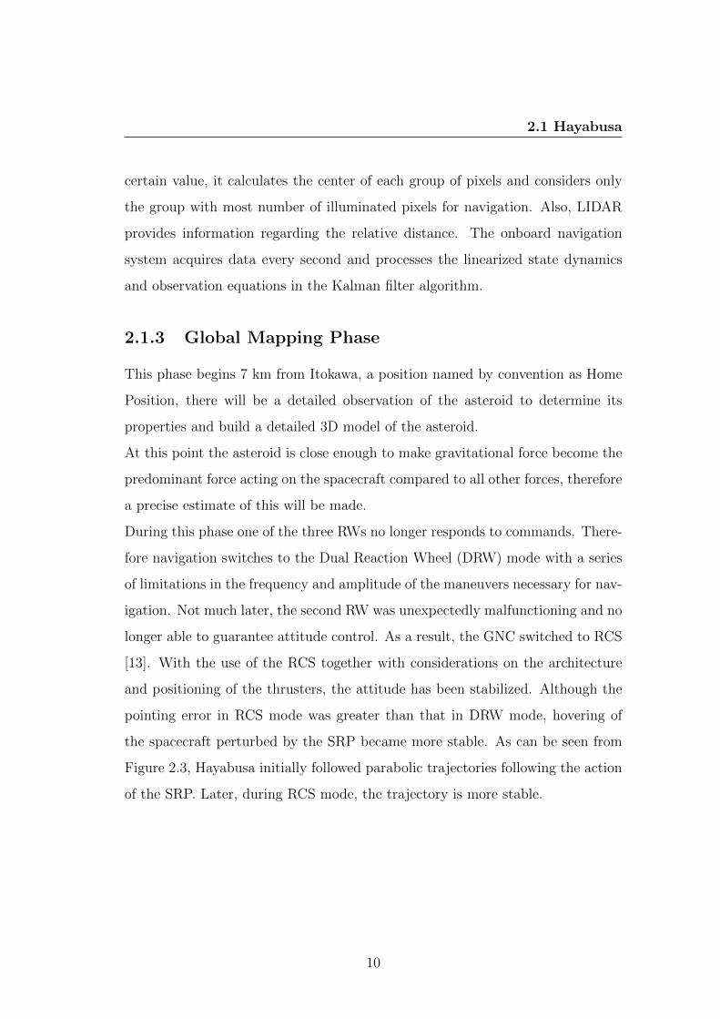
the spacecraft perturbed by the SRP became more stable. As can be seen from
Figure 2.3, Hayabusa initially followed parabolic trajectories following the action
of the SRP. Later, during RCS mode, the trajectory is more stable.
10
2.1 Hayabusa
Figure 2.3: The Z position historySource: [10],p.5
2.1.4 AOCS and GNC System
During the design of the mission, the dimensions, the shape and the surface
conformation of the asteroid were unknown. Therefore these variables had to be
taken into consideration and a more general GNC system had to be designed.
Figure 2.4: Block Diagram of AOCS/GNC SystemSource: [2],p.2
11
2.1 Hayabusa
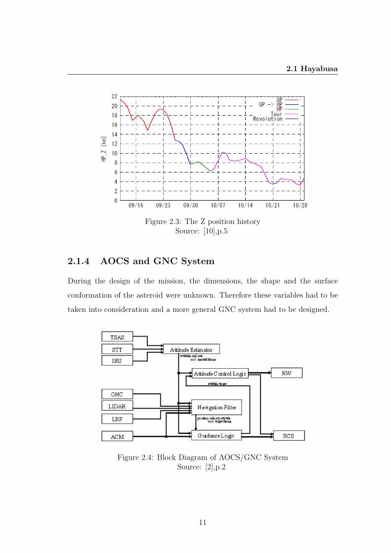
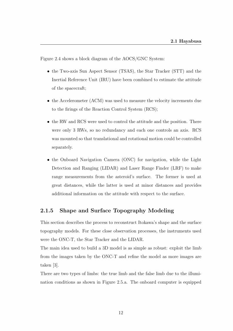
Figure 2.4 shows a block diagram of the AOCS/GNC System:
• the Two-axis Sun Aspect Sensor (TSAS), the Star Tracker (STT) and the
Inertial Reference Unit (IRU) have been combined to estimate the attitude
of the spacecraft;
• the Accelerometer (ACM) was used to measure the velocity increments due
to the firings of the Reaction Control System (RCS);
• the RW and RCS were used to control the attitude and the position. There
were only 3 RWs, so no redundancy and each one controls an axis. RCS
was mounted so that translational and rotational motion could be controlled
separately.
• the Onboard Navigation Camera (ONC) for navigation, while the Light
Detection and Ranging (LIDAR) and Laser Range Finder (LRF) to make
range measurements from the asteroid’s surface. The former is used at
great distances, while the latter is used at minor distances and provides
additional information on the attitude with respect to the surface.
2.1.5 Shape and Surface Topography Modeling
This section describes the process to reconstruct Itokawa’s shape and the surface
topography models. For these close observation processes, the instruments used
were the ONC-T, the Star Tracker and the LIDAR.
The main idea used to build a 3D model is as simple as robust: exploit the limb
from the images taken by the ONC-T and refine the model as more images are
taken [3].
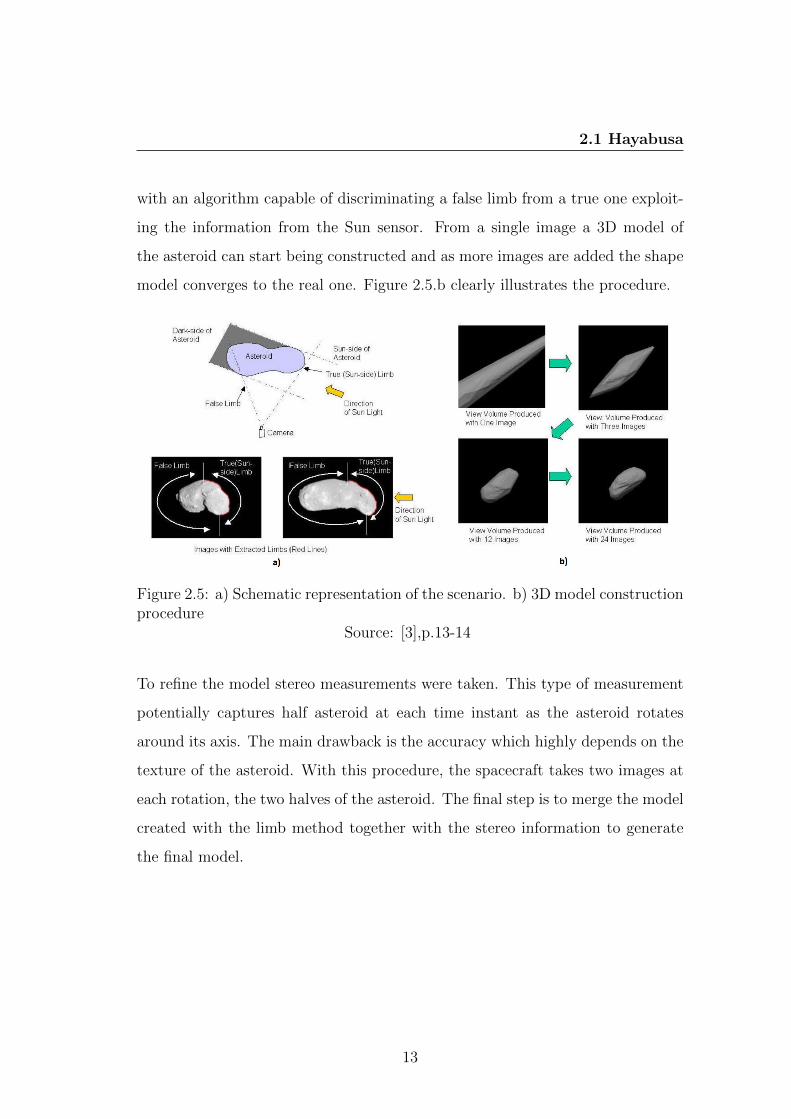
There are two types of limbs: the true limb and the false limb due to the illumi-
nation conditions as shown in Figure 2.5.a. The onboard computer is equipped
12
2.1 Hayabusa
with an algorithm capable of discriminating a false limb from a true one exploit-
ing the information from the Sun sensor. From a single image a 3D model of
the asteroid can start being constructed and as more images are added the shape
model converges to the real one. Figure 2.5.b clearly illustrates the procedure.
Figure 2.5: a) Schematic representation of the scenario. b) 3D model constructionprocedure
Source: [3],p.13-14
To refine the model stereo measurements were taken. This type of measurement
potentially captures half asteroid at each time instant as the asteroid rotates
around its axis. The main drawback is the accuracy which highly depends on the
texture of the asteroid. With this procedure, the spacecraft takes two images at
each rotation, the two halves of the asteroid. The final step is to merge the model
created with the limb method together with the stereo information to generate
the final model.
13
2.2 Rosetta
2.2 Rosetta
Rosetta is an ESA mission whose task was to encounter the comet 67P/Churyumov-
Gerasimenko. The mission was launched in 2004 and reached the comet in 2014.
This mission demonstrated the following procedures:
• first spacecraft to orbit a comet;
• first spacecraft to deploy and land a lander on the surface of a comet;
• first detection of organic particles on a comet;
2.2.1 Approach Phase
The first task was to detect the comet using the onboard cameras. Rosetta was
equipped with two identical NAVCAMs, the primary instruments for optical nav-
igation, and two OSIRIS cameras: a Narrow Angle Camera (NAC) and a Wide
Angle Camera (WAC).
At the beginning, the team tried to detect the comet using the NAVCAMs. The
position of the comet was known with an uncertainty of 15000 km, so both cam-
eras were pointed in the predicted direction. However, OSIRIS NAC was much
more sensitive, so it was also used for detection. Finally, at a distance of 4.9
million km, the comet was detected. To refine the position and orbit prediction
of the comet, every three days, three NAC images were taken and finally the
position was refined with an uncertainty of 2000 km. This procedure was carried
out until 1.8 million km when the NAVCAMs detected the comet.
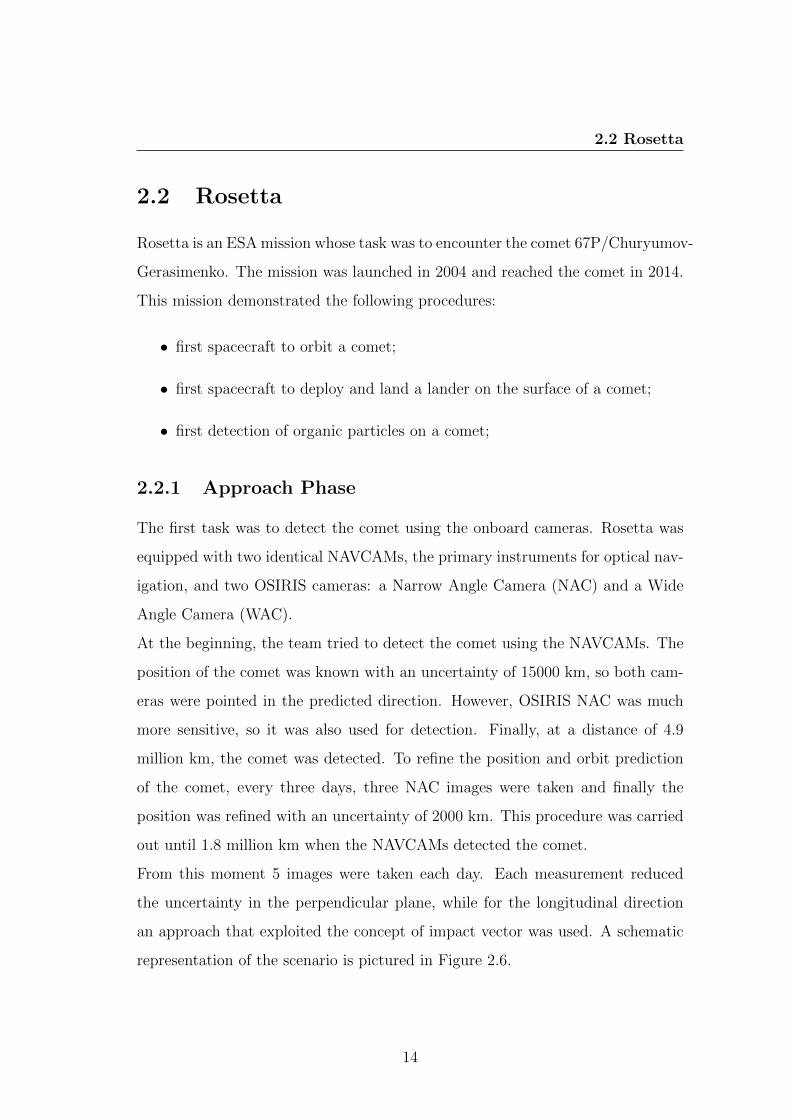
From this moment 5 images were taken each day. Each measurement reduced
the uncertainty in the perpendicular plane, while for the longitudinal direction
an approach that exploited the concept of impact vector was used. A schematic
representation of the scenario is pictured in Figure 2.6.
14
2.2 Rosetta
Figure 2.6: Effect of impact vector on navigation accuracySource: [14],p.6
When the impact vector is large the uncertainty related to these measurements is
small and viceversa. The limit case is when the impact vector is zero. In this case,
the relative distance does not improve by optical measurements. This concept
can be noticed in Figure 2.6 where the yellow area is the uncertainty related to a
certain impact vector.
2.2.2 Initial Characterization Phase
The first orbital strategy proposed to characterize the comet through circular
orbit was not adequate since:
• the estimate of the gravity field was affected by a great uncertainty at that
point;
• the spacecraft had a greater velocity than the escape velocity. Errors in the
orbit insertion would determine a trajectory completely different from the
designed one;
• the magnitude of the circular orbit velocity is small, so, to get images at
different illumination condition would have implied a longer phase duration.
The approach to the comet through hyperbolic arcs enjoys the following advan-
tages.
• They are not sensitive to gravitational estimation errors;
15
2.2 Rosetta
• There is a rapid excursion around the comet;
• The trajectories can be designed to face constantly the dayside.
The spacecraft flight was performed through hyperbolic arcs at low phase angles
providing a good view of the celestial body. In this phase, the first landmarks
were processed.
2.2.3 Global Mapping Phase
The spacecraft began flying 30 km orbits with larger phase angles. The goal in
this phase was to map up to 80% of the surface of the comet with a 2000 pixel
resolution and to cover it with landmarks. Additionally, the knowledge of the
comet dynamic and kinematic state was improved. The selected trajectory for
this phase was formed combining two 30 km orbits tilted by 30◦. To make an
excursion to the night side is sufficient to avoid making the maneuver at the pole,
however, it is preferable to keep the spacecraft in the dayside.
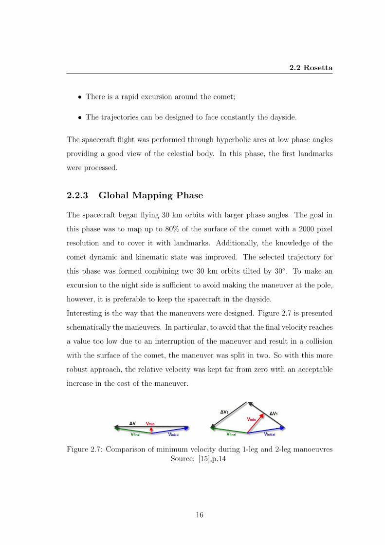
Interesting is the way that the maneuvers were designed. Figure 2.7 is presented
schematically the maneuvers. In particular, to avoid that the final velocity reaches
a value too low due to an interruption of the maneuver and result in a collision
with the surface of the comet, the maneuver was split in two. So with this more
robust approach, the relative velocity was kept far from zero with an acceptable
increase in the cost of the maneuver.
Figure 2.7: Comparison of minimum velocity during 1-leg and 2-leg manoeuvresSource: [15],p.14
16
2.2 Rosetta
2.2.4 Shape Modeling
Before the hibernation, Rosetta flew-by the asteroids 2867 Steins and 21 Lutetia
and had to characterize their shape. The fly-by of the first asteroid was conducted
successfully, but was affected by pointing issues that were solved for the fly-by
around 21 Lutetia. For the shape reconstruction of both asteroids the Silhouette
and the Shadow Carving Methods [16] [17] were adopted.
The first step was to pre-process the images filtering out the bright pixels not
belonging to the asteroid and correct the camera distortions.
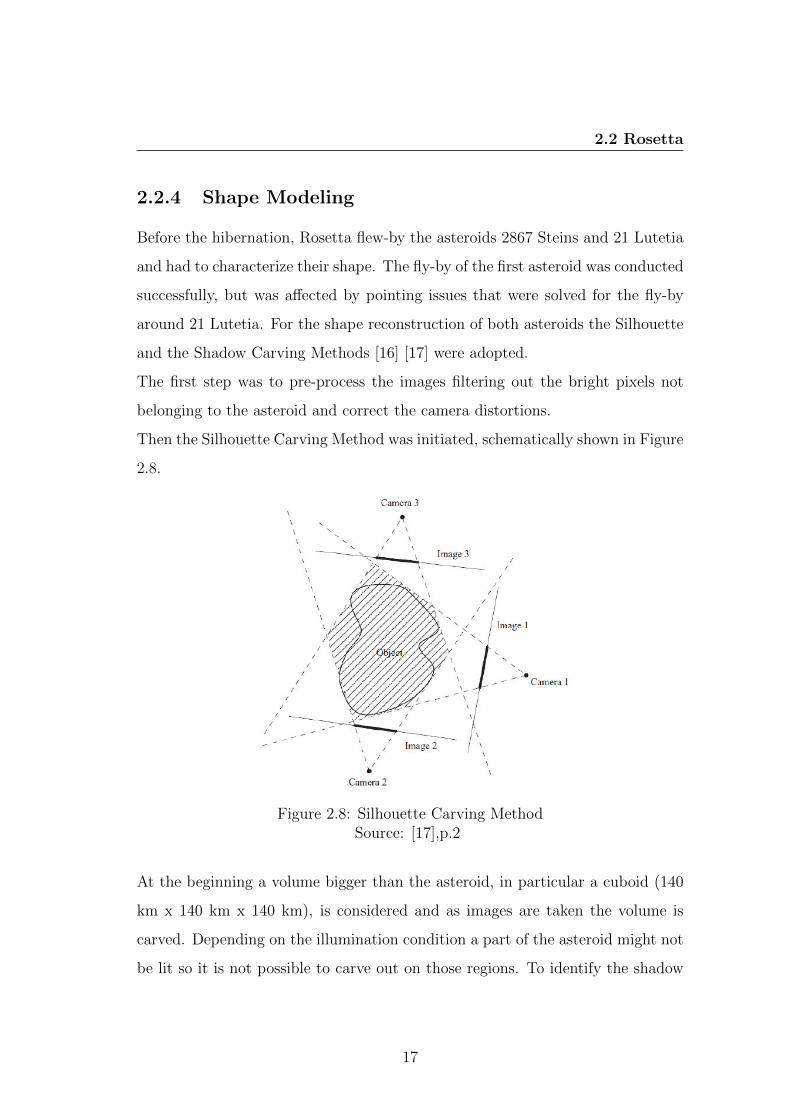
Then the Silhouette Carving Method was initiated, schematically shown in Figure
2.8.
Figure 2.8: Silhouette Carving MethodSource: [17],p.2
At the beginning a volume bigger than the asteroid, in particular a cuboid (140
km x 140 km x 140 km), is considered and as images are taken the volume is
carved. Depending on the illumination condition a part of the asteroid might not
be lit so it is not possible to carve out on those regions. To identify the shadow
17
2.2 Rosetta
side from the empty space region, pixels were classified as three types:
• lit, pixels bright over a certain threshold;
• candidate, pixels candidate to be part of the shadow region. To ensure this
the Sun direction is continuously tracked;
• empty, all the rest of the pixels.
In the last phase, the Shadow Carving Method was used to resolve the lit/shadow
contradictions between the model and the images. After this process the model
becomes photoconsistent. With this last method, once the spacecraft has a good
view of the asteroid and has enough data about the Sun-asteroid-spacecraft con-
figuration, the concave regions, that cannot be modeled with the Silhouette Carv-
ing Method, can be solved.
Once this prototype program has been successfully used for Lutetia, it was also
used for the characterization of the comet 67P/Churyumov-Gerasimenko.
18
Chapter 3
System’s Architecture and
Dynamic Models
Summary
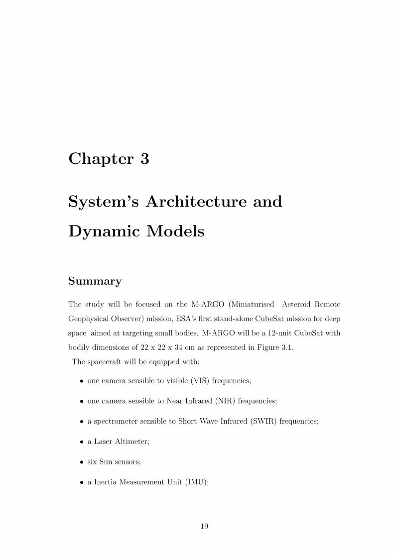
The study will be focused on the M-ARGO (Miniaturised Asteroid Remote
Geophysical Observer) mission, ESA’s first stand-alone CubeSat mission for deep
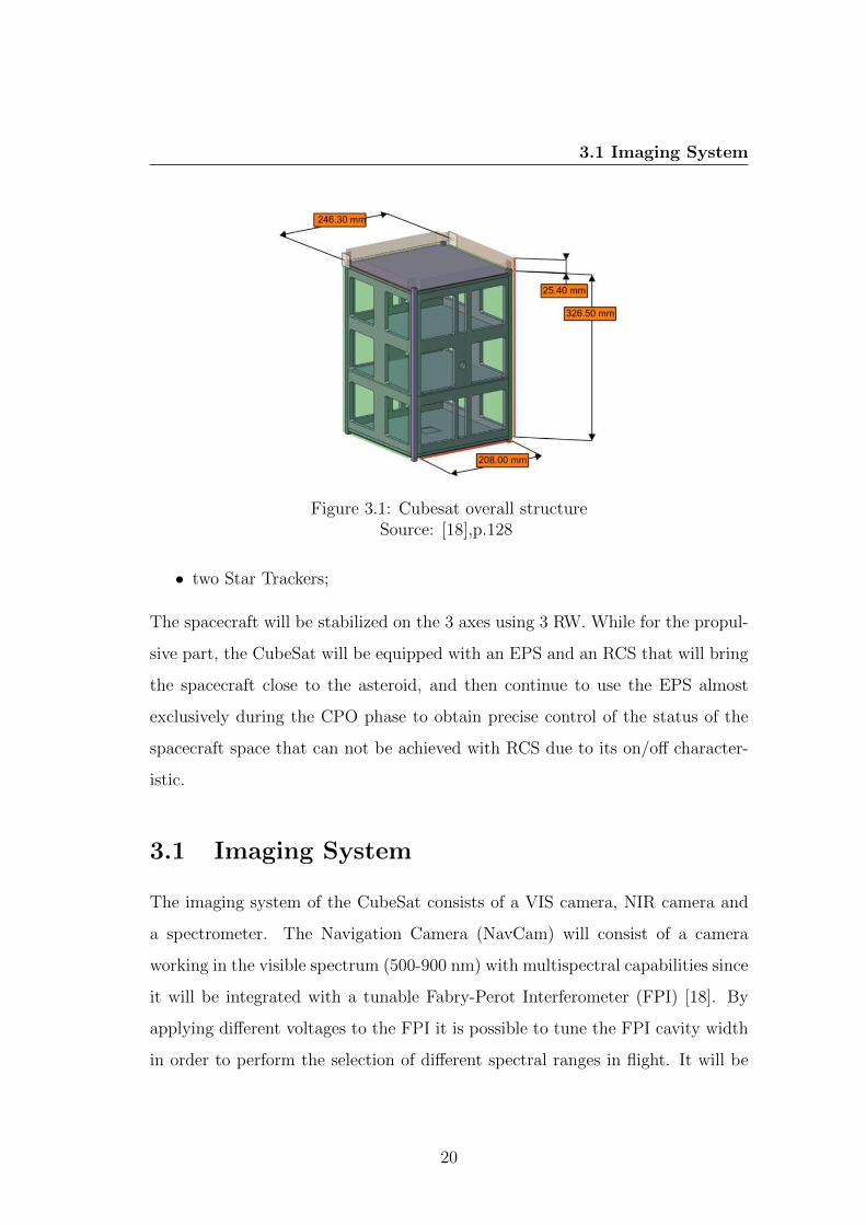
space aimed at targeting small bodies. M-ARGO will be a 12-unit CubeSat with
bodily dimensions of 22 x 22 x 34 cm as represented in Figure 3.1.
The spacecraft will be equipped with:
• one camera sensible to visible (VIS) frequencies;
• one camera sensible to Near Infrared (NIR) frequencies;
• a spectrometer sensible to Short Wave Infrared (SWIR) frequencies;
• a Laser Altimeter;
• six Sun sensors;
• a Inertia Measurement Unit (IMU);
19
3.1 Imaging System
Figure 3.1: Cubesat overall structureSource: [18],p.128
• two Star Trackers;
The spacecraft will be stabilized on the 3 axes using 3 RW. While for the propul-
sive part, the CubeSat will be equipped with an EPS and an RCS that will bring
the spacecraft close to the asteroid, and then continue to use the EPS almost
exclusively during the CPO phase to obtain precise control of the status of the
spacecraft space that can not be achieved with RCS due to its on/off character-
istic.
3.1 Imaging System
The imaging system of the CubeSat consists of a VIS camera, NIR camera and
a spectrometer. The Navigation Camera (NavCam) will consist of a camera
working in the visible spectrum (500-900 nm) with multispectral capabilities since
it will be integrated with a tunable Fabry-Perot Interferometer (FPI) [18]. By
applying different voltages to the FPI it is possible to tune the FPI cavity width
in order to perform the selection of different spectral ranges in flight. It will be
20
3.1 Imaging System
used for asteroid detection, navigation, to create landmarks on the surface of the
asteroid and a 3D model of it. It is characterized by the following parameters:
• Field of View: 6◦ × 6◦ ;
• Image Size: 1024× 1024;
• Pixel Size: 5.5× 5.5 µm2;
• Focal Length: 32.3 mm;
• Ground Sample Distance (GSD) at 500 m: 9 cm;
• SNR: 40;
The NIRCam detects the 900-1600 nm range of frequencies, capable of acquir-
ing multispectra images. It will be used together with the visible camera for
navigation purposes. It is characterized by the following parameters:
• Field of View: 5.3◦ × 5.3◦ ;
• Image Size: 256× 256;
• Pixel Size: 30× 30 µm2;
• Focal Length: 81.5 mm;
• Ground Sample Distance (GSD) at 500 m: 18 cm;
• SNR: 40;
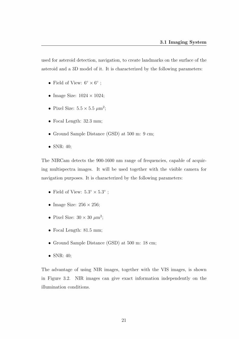
The advantage of using NIR images, together with the VIS images, is shown
in Figure 3.2. NIR images can give exact information independently on the
illumination conditions.
21
3.1 Imaging System
Figure 3.2: Performance comparison between visible and IR camerasSource: NASA / JPL
The SWIR optical spectrometer will be used for chemical composition analysis
of the asteroids. It uses the phenomenon of optical dispersion. The light from a
source can consist of a continuous spectrum, an emission spectrum or an absorp-
tion spectrum. Because each element leaves its spectral signature in the pattern
of lines observed, spectral analysis can reveal the composition of the object be-
ing analyzed. For a detailed description of the SWIR spectrometer architecture
and functioning refer to [19] and [20]. In particular, the spectrometer installed is
sensible to the 1600-2500 nm range of frequency and has the following specifics:
• Field of View: 5◦ circular;
• Image Size: 1 pixel;
• Pixel Size: 1000× 1000 µm2;
• Focal Length: 11.7 mm;
• Ground Sample Distance (GSD) at 500 m: 44 m;
• SNR: 100;
22
3.2 Asteroids
3.2 Asteroids
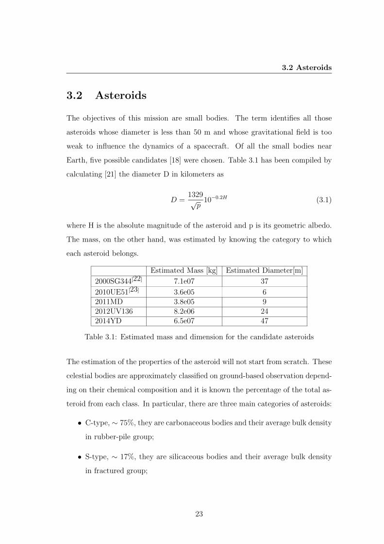
The objectives of this mission are small bodies. The term identifies all those
asteroids whose diameter is less than 50 m and whose gravitational field is too
weak to influence the dynamics of a spacecraft. Of all the small bodies near
Earth, five possible candidates [18] were chosen. Table 3.1 has been compiled by
calculating [21] the diameter D in kilometers as
D =1329√p
10−0.2H (3.1)
where H is the absolute magnitude of the asteroid and p is its geometric albedo.
The mass, on the other hand, was estimated by knowing the category to which
each asteroid belongs.
Estimated Mass [kg] Estimated Diameter[m]
2000SG344[22] 7.1e07 37
2010UE51[23] 3.6e05 62011MD 3.8e05 92012UV136 8.2e06 242014YD 6.5e07 47
Table 3.1: Estimated mass and dimension for the candidate asteroids
The estimation of the properties of the asteroid will not start from scratch. These
celestial bodies are approximately classified on ground-based observation depend-
ing on their chemical composition and it is known the percentage of the total as-
teroid from each class. In particular, there are three main categories of asteroids:
• C-type, ∼ 75%, they are carbonaceous bodies and their average bulk density
in rubber-pile group;
• S-type, ∼ 17%, they are silicaceous bodies and their average bulk density
in fractured group;
23
3.2 Asteroids
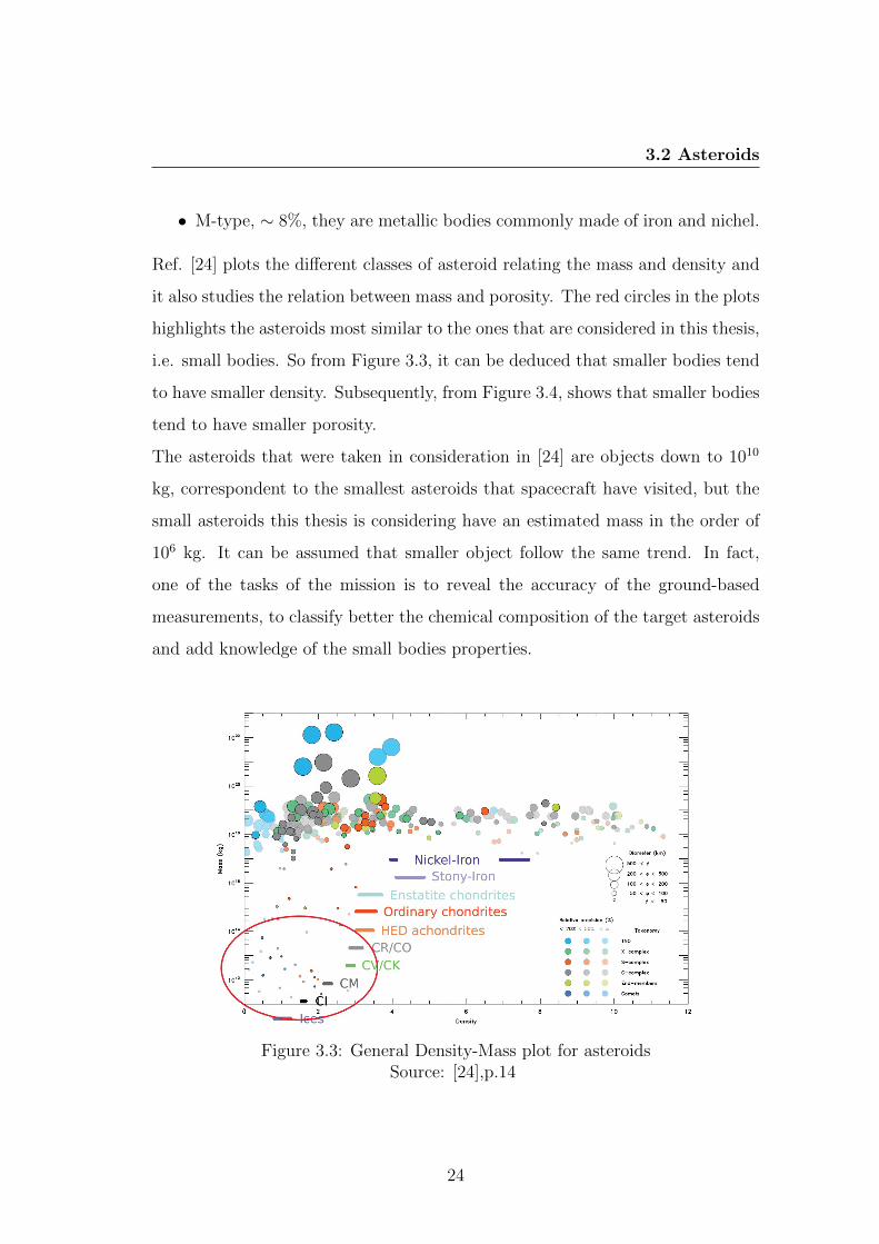
• M-type, ∼ 8%, they are metallic bodies commonly made of iron and nichel.
Ref. [24] plots the different classes of asteroid relating the mass and density and
it also studies the relation between mass and porosity. The red circles in the plots
highlights the asteroids most similar to the ones that are considered in this thesis,
i.e. small bodies. So from Figure 3.3, it can be deduced that smaller bodies tend
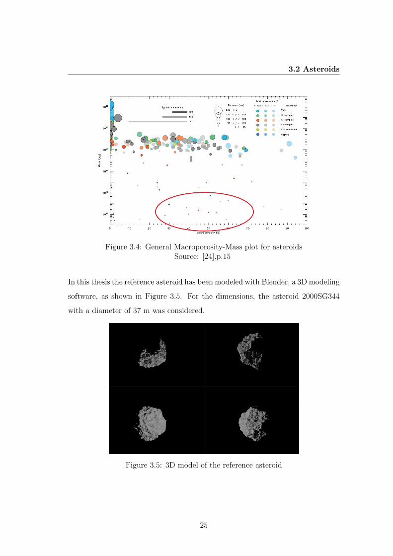
to have smaller density. Subsequently, from Figure 3.4, shows that smaller bodies
tend to have smaller porosity.
The asteroids that were taken in consideration in [24] are objects down to 1010
kg, correspondent to the smallest asteroids that spacecraft have visited, but the
small asteroids this thesis is considering have an estimated mass in the order of
106 kg. It can be assumed that smaller object follow the same trend. In fact,
one of the tasks of the mission is to reveal the accuracy of the ground-based
measurements, to classify better the chemical composition of the target asteroids
and add knowledge of the small bodies properties.
Figure 3.3: General Density-Mass plot for asteroidsSource: [24],p.14
24
3.2 Asteroids
Figure 3.4: General Macroporosity-Mass plot for asteroidsSource: [24],p.15
In this thesis the reference asteroid has been modeled with Blender, a 3D modeling
software, as shown in Figure 3.5. For the dimensions, the asteroid 2000SG344
with a diameter of 37 m was considered.
Figure 3.5: 3D model of the reference asteroid
25
3.2 Asteroids
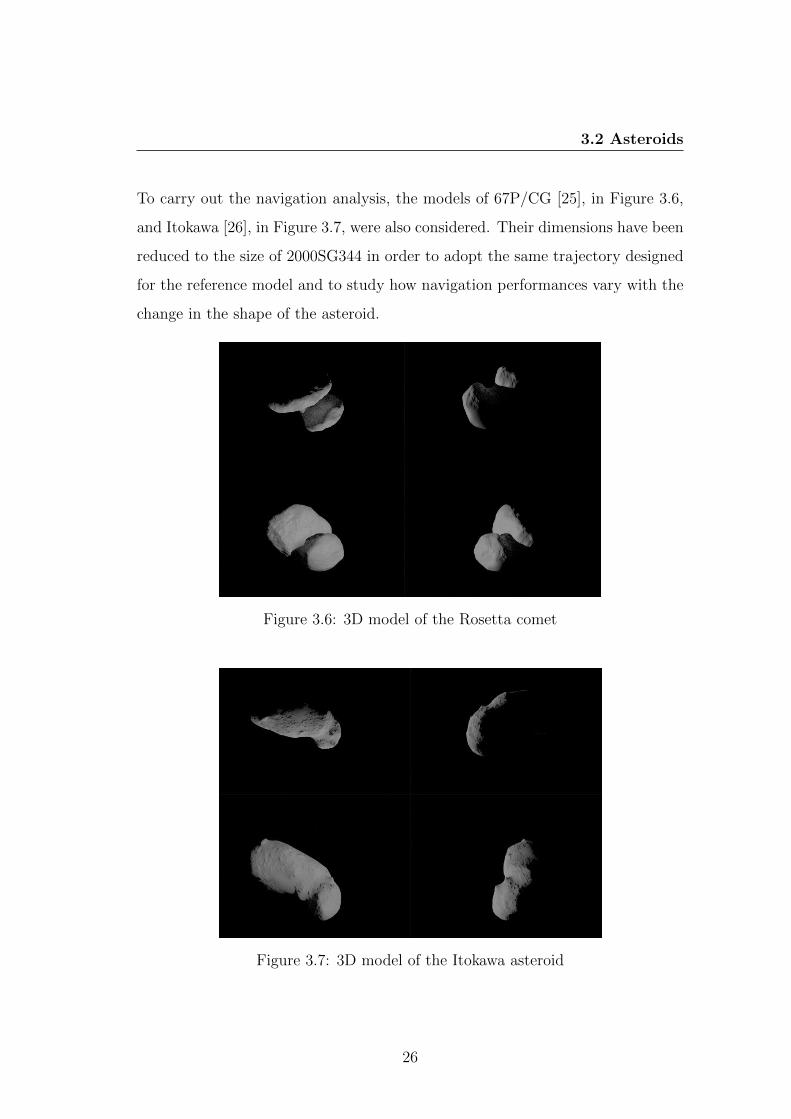
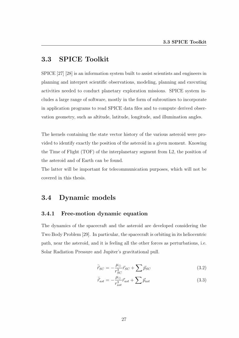
To carry out the navigation analysis, the models of 67P/CG [25], in Figure 3.6,
and Itokawa [26], in Figure 3.7, were also considered. Their dimensions have been
reduced to the size of 2000SG344 in order to adopt the same trajectory designed
for the reference model and to study how navigation performances vary with the
change in the shape of the asteroid.
Figure 3.6: 3D model of the Rosetta comet
Figure 3.7: 3D model of the Itokawa asteroid
26
3.3 SPICE Toolkit
3.3 SPICE Toolkit
SPICE [27] [28] is an information system built to assist scientists and engineers in
planning and interpret scientific observations, modeling, planning and executing
activities needed to conduct planetary exploration missions. SPICE system in-
cludes a large range of software, mostly in the form of subroutines to incorporate
in application programs to read SPICE data files and to compute derived obser-
vation geometry, such as altitude, latitude, longitude, and illumination angles.
The kernels containing the state vector history of the various asteroid were pro-
vided to identify exactly the position of the asteroid in a given moment. Knowing
the Time of Flight (TOF) of the interplanetary segment from L2, the position of
the asteroid and of Earth can be found.
The latter will be important for telecommunication purposes, which will not be
covered in this thesis.
3.4 Dynamic models
3.4.1 Free-motion dynamic equation
The dynamics of the spacecraft and the asteroid are developed considering the
Two Body Problem [29]. In particular, the spacecraft is orbiting in its heliocentric
path, near the asteroid, and it is feeling all the other forces as perturbations, i.e.
Solar Radiation Pressure and Jupiter’s gravitational pull.
~rSC = − µ�
r3SC~rSC +
∑~pSC (3.2)
~rast = − µ�
r3ast~rast +
∑~past (3.3)
27
3.4 Dynamic models
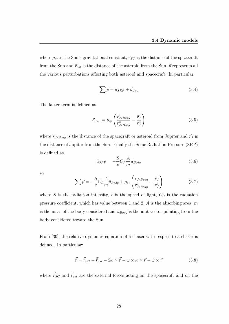
where µ� is the Sun’s gravitational constant, ~rSC is the distance of the spacecraft
from the Sun and ~rast is the distance of the asteroid from the Sun, ~p represents all
the various perturbations affecting both asteroid and spacecraft. In particular:
∑~p = ~aSRP + ~aJup (3.4)
The latter term is defined as
~aJup = µ�
(~rJ/Body
r3J/Body
− ~rJr3J
)(3.5)
where ~rJ/Body is the distance of the spacecraft or asteroid from Jupiter and ~rJ is
the distance of Jupiter from the Sun. Finally the Solar Radiation Pressure (SRP)
is defined as
~aSRP = −ScCR
A
muBody (3.6)
so ∑~p = −S
cCR
A
muBody + µ�
(~rJ/Body
r3J/Body
− ~rJr3J
)(3.7)
where S is the radiation intensity, c is the speed of light, CR is the radiation
pressure coefficient, which has value between 1 and 2, A is the absorbing area, m
is the mass of the body considered and uBody is the unit vector pointing from the
body considered toward the Sun.
From [30], the relative dynamics equation of a chaser with respect to a chaser is
defined. In particular:
~r = ~rSC − ~rast − 2ω × ~r − ω × ω × ~r − ω × ~r (3.8)
where ~rSC and ~rast are the external forces acting on the spacecraft and on the
28

3.4 Dynamic models
asteroid with respect to the frame of the asteroid, ω and ω are the angular velocity
and angular acceleration of the asteroid frame with respect to the inertial frame.
In our case the body frame is considered fixed with respect to the inertial frame,
so ω = ω = 0. With this consideration, the relative dynamics equation simplifies
to
~r = ~rSC − ~rast = (3.9)
= − µ�
r3SC~rSC +
∑~pSC − (− µ�
r3ast~rast +
∑~past) (3.10)
making explicit every term
~r = − µ�
r3SC~rSC −
S
cCR
ASC
mSC
uSC + µ�
(~rJ/SCr3J/SC
− ~rJr3J
)−(
− µ�
r3ast~rast −
S
cCR
Aast
mast
uast + µ�
(~rJ/astr3J/ast
− ~rJr3J
)) (3.11)
During CPO the following assumptions are valid
~rSC ∼ ~rast , ~rJ/SC ∼ ~rJ/ast and uSC ∼ uast (3.12)
So the dynamics reduces to
~r =
(−ScCR
ASC
mSC
+S
cCR
Aast
mast
)uSC (3.13)
This is the dynamic equation describing the Free-Thrust motion.
3.4.2 Complete equation of motion
To address the spacecraft into the nominal path the system employs low-thrust
engine modelled as finite maneuvers. The amplitude of the acceleration due to the
29
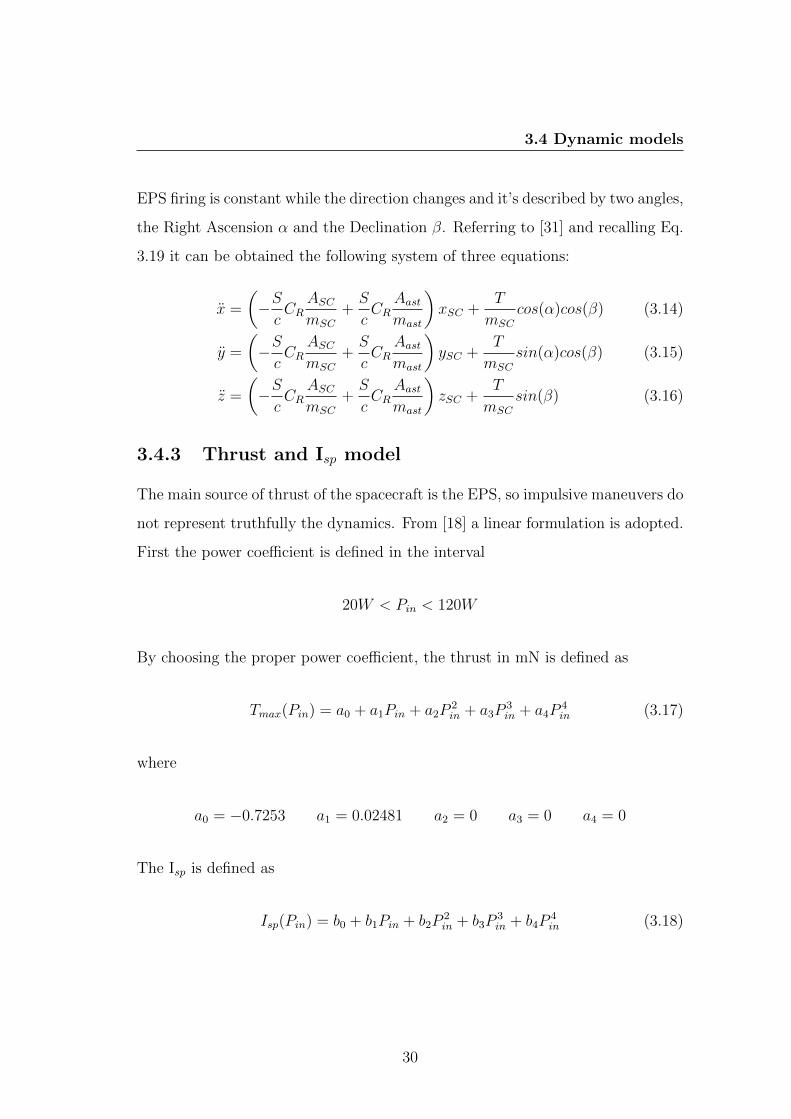
3.4 Dynamic models
EPS firing is constant while the direction changes and it’s described by two angles,
the Right Ascension α and the Declination β. Referring to [31] and recalling Eq.
3.19 it can be obtained the following system of three equations:
x =
(−ScCR
ASC
mSC
+S
cCR
Aast
mast
)xSC +
T
mSC
cos(α)cos(β) (3.14)
y =
(−ScCR
ASC
mSC
+S
cCR
Aast
mast
)ySC +
T
mSC
sin(α)cos(β) (3.15)
z =
(−ScCR
ASC
mSC
+S
cCR
Aast
mast
)zSC +
T
mSC
sin(β) (3.16)
3.4.3 Thrust and Isp model
The main source of thrust of the spacecraft is the EPS, so impulsive maneuvers do
not represent truthfully the dynamics. From [18] a linear formulation is adopted.
First the power coefficient is defined in the interval
20W < Pin < 120W
By choosing the proper power coefficient, the thrust in mN is defined as
Tmax(Pin) = a0 + a1Pin + a2P2in + a3P
3in + a4P
4in (3.17)
where
a0 = −0.7253 a1 = 0.02481 a2 = 0 a3 = 0 a4 = 0
The Isp is defined as
Isp(Pin) = b0 + b1Pin + b2P2in + b3P
3in + b4P
4in (3.18)
30
3.5 CPO Calculator
where
b0 = 2652 b1 = −18.123 b2 = 0.3887 b3 = −0.00174 b4 = 0
3.5 CPO Calculator
The problem of designing the orbit was to obtain the velocity needed to go from
one vertex to another respecting time and position constraints. It is similar to a
Lambert problem since the input data is the starting position, the final one and
the interval of time to go from one point to another. Nevertheless the solution
of this well-known problem could not be used since the motion was affected by
disturbances. For this reason, the Shooting Method was adopted. To start using
the method an initial estimate of the velocity is needed, so by using kinematics
laws the initial guess could be determined.
In Section 3.4.1 it has been defined that the dynamics were characterized by
presence of the SRP
~r =
(−ScCR
ASC
mSC
+S
cCR
Aast
mast
)uSC (3.19)
~r = aSRPTOTuSC (3.20)
The module of this acceleration is constant since the distance does not change
significantly, but the direction does change as the asteroid rotates around the
Sun.
So the motion can be approximated as a uniformly accelerated motion in all the
directions.
31
3.5 CPO Calculator
Considering the x direction, the motion is described by Equation 3.21.
∆x = vx0∆t+1
2ax∆t2 (3.21)
where ∆x is the difference of the x coordinate of the two vertices, ∆t the duration
of the segment and ax is the total SRP acting on the spacecraft on the x-direction.
To compute the ax, the direction of the Sun is needed. As an approximation the
direction of the Sun during the segment will be considered constant and it will
be computed as the mean position from the starting vertex to the ending one.
As the direction has been determined
ax = aSRPTOTxSC (3.22)
and the vx0 can be computed from Equation 3.21. The same procedure will be
adopted also in the y- and z-direction. The dynamics will be propagated using a
velocity below the one estimated and a velocity greater than the estimated one,
then, via interpolation, the velocity needed to reach the exact vertex can be found.
A CPO simulator was developed to allow to simulate CPO in different conditions.
The main parameters that can be modified during the trajectory design are:
the maximum phase angle that the spacecraft can reach; the length and the
duration of each segments; the total flight time; the shape of the trajectory. Each
parameter improves or worsens the final result and some go against each other,
therefore a trade-off analysis is necessary to obtain an optimal result. The main
objective is to reduce as much as possible the cost of the single maneuver is the
monthly cost of the mission.
A screenshot of the CPO Calculator software is reported in Figure 3.8.
32
3.5 CPO Calculator
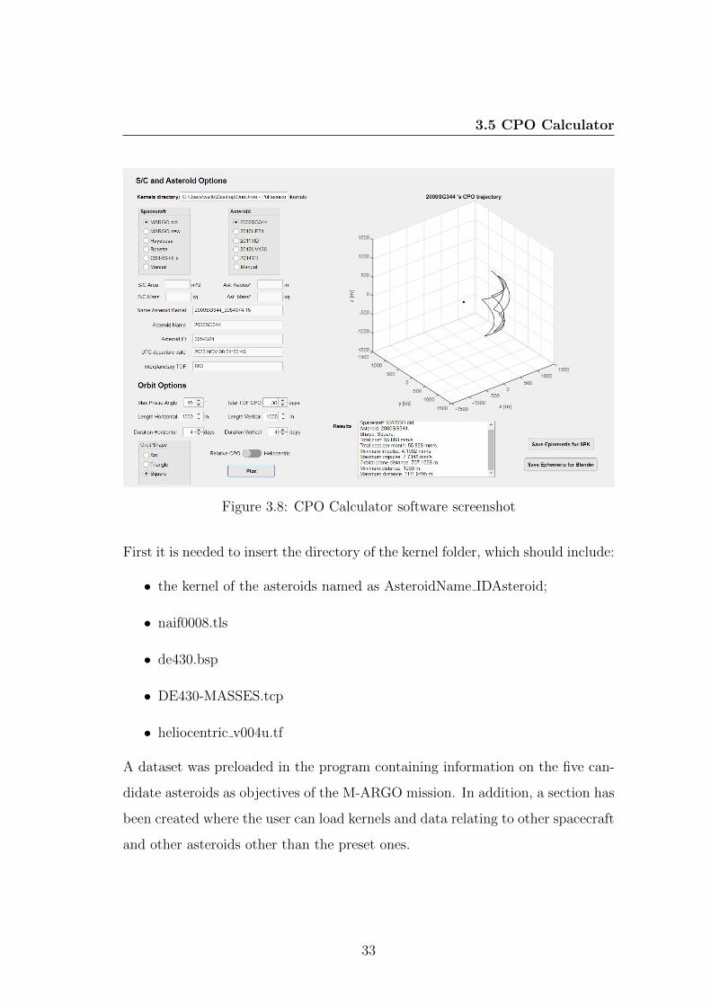
Figure 3.8: CPO Calculator software screenshot
First it is needed to insert the directory of the kernel folder, which should include:
• the kernel of the asteroids named as AsteroidName IDAsteroid;
• naif0008.tls
• de430.bsp
• DE430-MASSES.tcp
• heliocentric v004u.tf
A dataset was preloaded in the program containing information on the five can-
didate asteroids as objectives of the M-ARGO mission. In addition, a section has
been created where the user can load kernels and data relating to other spacecraft
and other asteroids other than the preset ones.
33
3.5 CPO Calculator
Once the spacecraft and the asteroid have been defined, it will be possible to set
the different parameters, keeping in mind the considerations that will be reported
at the end of this section. Once all the parameters have been defined, it will be
possible to plot or the heliocentric view of the orbits of the earth and the asteroid
with a view of the position of the two celestial bodies at the beginning and end
of the CPO or it will be possible to plot the trajectories of the spacecraft relative
to the asteroid that will be depicted in scale.
More importantly, the results that the program will report in the Results area
will be: the information regarding the spacecraft, the asteroid, the shape chosen
for the trajectory, the minimum cost and the maximum cost of the individual
pulses, the monthly cost and the minimum distance and the maximum distance
from the asteroid.
Finally, the ephemerides related to the trajectory can be saved in a text file in
order to generate an SPK file or to be able to use them in the Blender program
for more realistic simulations and for the implementation of an optical navigation
algorithm that will be presented in the next section.
Generally, by changing one parameter at a time, the following consideration can
be made:
• increasing the maximum phase angle the distance decreases and the impulse
cost doesn’t change;
• increasing the length of the segments it decreases the concavity of the tra-
jectory, making it flatter, the distance from the asteroid increases and the
cost slightly increases;
• increasing the duration of the segments it increases the concavity of the
trajectory, it increases the segment cost, but the monthly budget lowers.
34
3.6 Vision-based Navigation Algorithm
3.6 Vision-based Navigation Algorithm
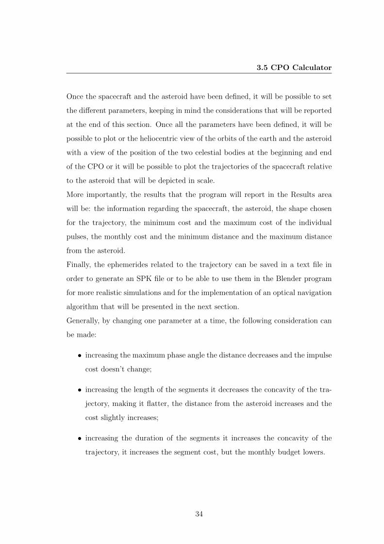
The Vision-based Navigation simulation will be implemented with the combined
use of MATLAB and Blender. The simulation will be schematically represented
in Figure 3.9.
Figure 3.9: Scheme of the test of the Navigation algorithm
• Once the orbital path for the R&CPO is developed, the ephemerides will
exported from MATLAB both for creating the SPK for SPICE and to be
imported in Blender;
• Then, in Blender, the spacecraft will be constrained to follow that path
keeping the asteroid in the FOV of the camera. This program will keep the
camera pointing at the asteroid’s CoM;
• Once the camera point of view has been rendered through a video, it will
be analized by MATLAB through a image processing algorithm.
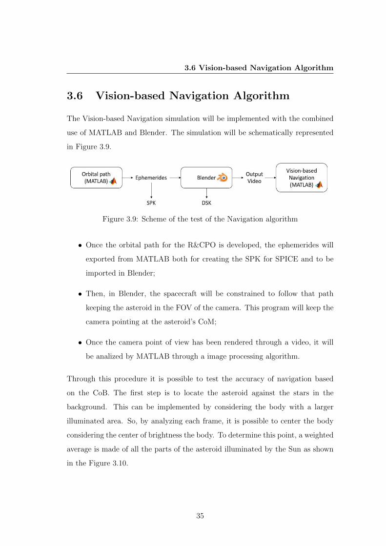
Through this procedure it is possible to test the accuracy of navigation based
on the CoB. The first step is to locate the asteroid against the stars in the
background. This can be implemented by considering the body with a larger
illuminated area. So, by analyzing each frame, it is possible to center the body
considering the center of brightness the body. To determine this point, a weighted
average is made of all the parts of the asteroid illuminated by the Sun as shown
in the Figure 3.10.
35
3.6 Vision-based Navigation Algorithm
Figure 3.10: Computation of the CoB
The algorithm will then be applied during navigation without knowing the CoM
and in the various phases of the R&CPO the error between the CoM and the
CoB will be analyzed, proposing a solution if the navigation based on the CoB is
affected by a not negligible error.
Finally, the accuracy of navigation will be assessed as the shape of the asteroid
changes. In the basic case, an asteroid of fairly regular shape was considered;
subsequently the case in which the asteroid has a more complex shape as the
asteroid Itokawa and the comet 67P/CG will be analyzed.
36
Chapter 4
Mission Design
Summary
The R&CPO segments will be divided into 4 phases according to which naviga-
tion instruments will be used. The four phases will be: the Absolute Navigation
(AbsNav) Phase, the Relative Navigation Part 1 (RelNav pt.1) Phase, the Rel-
ative Navigation Part 2 (RelNav pt.2) Phase, the Close Proximity Operations
(CPO) Phase.
The mission has the following requirements:
• The spacecraft shall rendezvous with the asteroid.
• The spacecraft shall determine the geophysical properties of the asteroid
and analyze the asteroids dynamic state.
• The spacecraft shall be properly disposed after it maps the asteroid and get
as many parameters as possible.
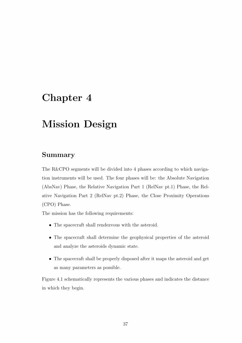
Figure 4.1 schematically represents the various phases and indicates the distance
in which they begin.
37
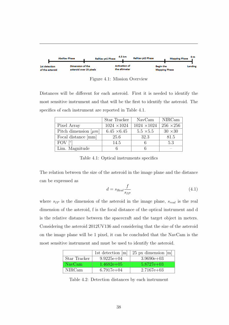
Figure 4.1: Mission Overview
Distances will be different for each asteroid. First it is needed to identify the
most sensitive instrument and that will be the first to identify the asteroid. The
specifics of each instrument are reported in Table 4.1.
Star Tracker NavCam NIRCamPixel Array 1024 ×1024 1024 ×1024 256 ×256Pitch dimension [µm] 6.45 ×6.45 5.5 ×5.5 30 ×30Focal distance [mm] 25.6 32.3 81.5FOV [◦] 14.5 6 5.3Lim. Magnitude 6 6 –
Table 4.1: Optical instruments specifics
The relation between the size of the asteroid in the image plane and the distance
can be expressed as
d = sRealf
sIP(4.1)
where sIP is the dimension of the asteroid in the image plane, sreal is the real
dimension of the asteroid, f is the focal distance of the optical instrument and d
is the relative distance between the spacecraft and the target object in meters.
Considering the asteroid 2012UV136 and considering that the size of the asteroid
on the image plane will be 1 pixel, it can be concluded that the NavCam is the
most sensitive instrument and must be used to identify the asteroid.
1st detection [m] 25 px dimension [m]Star Tracker 9.9225e+04 3.9690e+03NavCam 1.4682e+05 5.8727e+03NIRCam 6.7917e+04 2.7167e+03
Table 4.2: Detection distances by each instrument
38

The results are compared with Figure 4.2 and 4.3, from [18], that take as reference
asteroid 2012UV136. For the NavCam, that has a FOV of 6◦, the asteroid was
predicted to be visible at a distance of between 105 m and 6 × 10⁵ m, thus
confirming the analytically obtained results. Similarly, Figure 4.3 represents the
initial distance detection using the Star Tracker. In particular, the Star Tracker
considered has a FOV of 14.5◦and the figure indicates that the initial distance
detection may vary between 5× 10⁴ m and 2× 10⁵ m.
Figure 4.2: Initial distance asteroid detectability domain using NavCamSource: [18],p.191
Table 4.3 summarizes the distance information that were not made explicit in
Figure 4.1.
1st detection [m] 25 px dimension [m] CPO Phase [m]2000SG344 2.1729e+05 8.6916e+03 400 <d <8002010UE51 3.5236e+04 1.4095e+03 65 <d <1302011MD 5.2855e+04 2.1142e+03 97 <d <2002012UV136 1.4682e+05 5.8727e+03 270 <d <5402014YD 2.9364e+05 1.1745e+04 540 <d <1000
Table 4.3: M-ARGO mission distance milestones
39
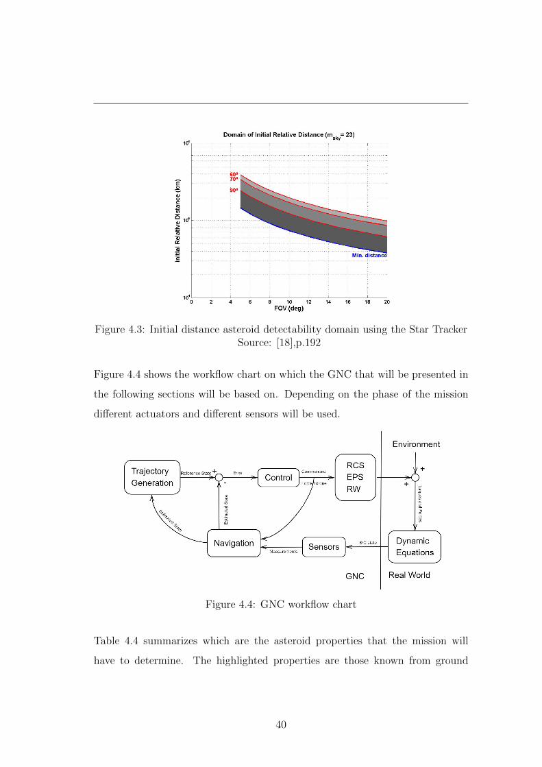
Figure 4.3: Initial distance asteroid detectability domain using the Star TrackerSource: [18],p.192
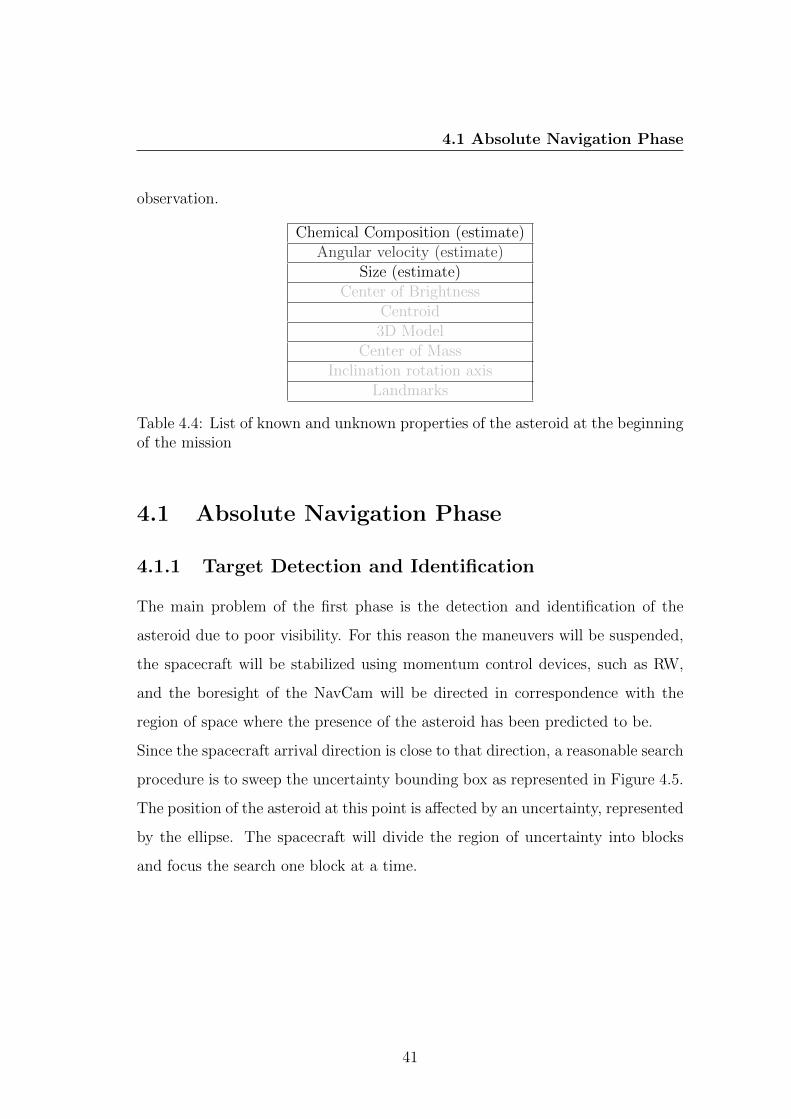
Figure 4.4 shows the workflow chart on which the GNC that will be presented in
the following sections will be based on. Depending on the phase of the mission
different actuators and different sensors will be used.
Figure 4.4: GNC workflow chart
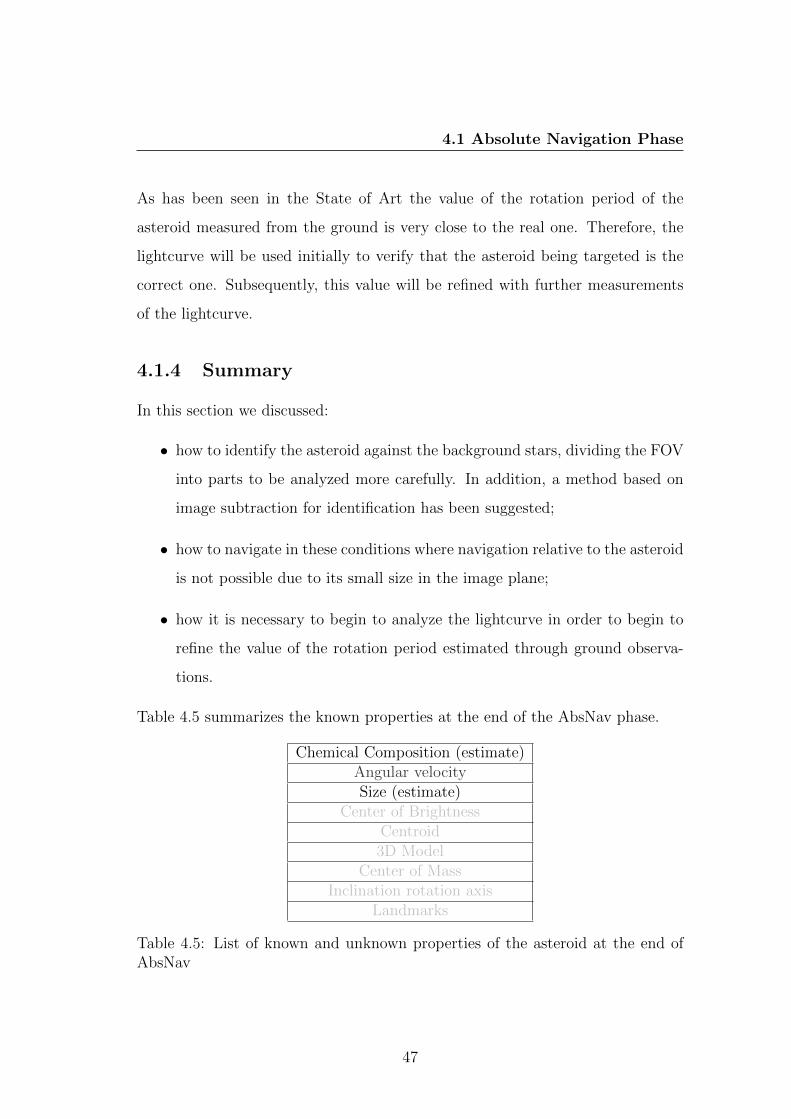
Table 4.4 summarizes which are the asteroid properties that the mission will
have to determine. The highlighted properties are those known from ground
40
4.1 Absolute Navigation Phase
observation.
Chemical Composition (estimate)Angular velocity (estimate)
Size (estimate)Center of Brightness
Centroid3D Model
Center of MassInclination rotation axis
Landmarks
Table 4.4: List of known and unknown properties of the asteroid at the beginningof the mission
4.1 Absolute Navigation Phase
4.1.1 Target Detection and Identification
The main problem of the first phase is the detection and identification of the
asteroid due to poor visibility. For this reason the maneuvers will be suspended,
the spacecraft will be stabilized using momentum control devices, such as RW,
and the boresight of the NavCam will be directed in correspondence with the
region of space where the presence of the asteroid has been predicted to be.
Since the spacecraft arrival direction is close to that direction, a reasonable search
procedure is to sweep the uncertainty bounding box as represented in Figure 4.5.
The position of the asteroid at this point is affected by an uncertainty, represented
by the ellipse. The spacecraft will divide the region of uncertainty into blocks
and focus the search one block at a time.
41
4.1 Absolute Navigation Phase
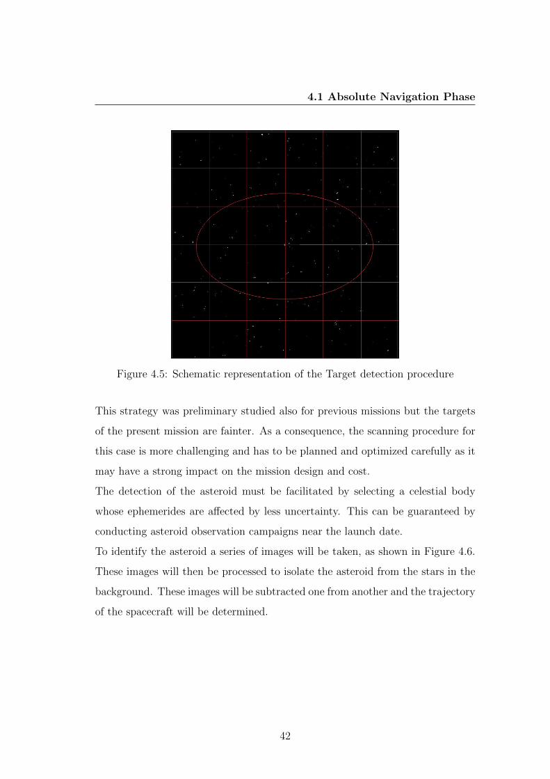
Figure 4.5: Schematic representation of the Target detection procedure
This strategy was preliminary studied also for previous missions but the targets
of the present mission are fainter. As a consequence, the scanning procedure for
this case is more challenging and has to be planned and optimized carefully as it
may have a strong impact on the mission design and cost.
The detection of the asteroid must be facilitated by selecting a celestial body
whose ephemerides are affected by less uncertainty. This can be guaranteed by
conducting asteroid observation campaigns near the launch date.
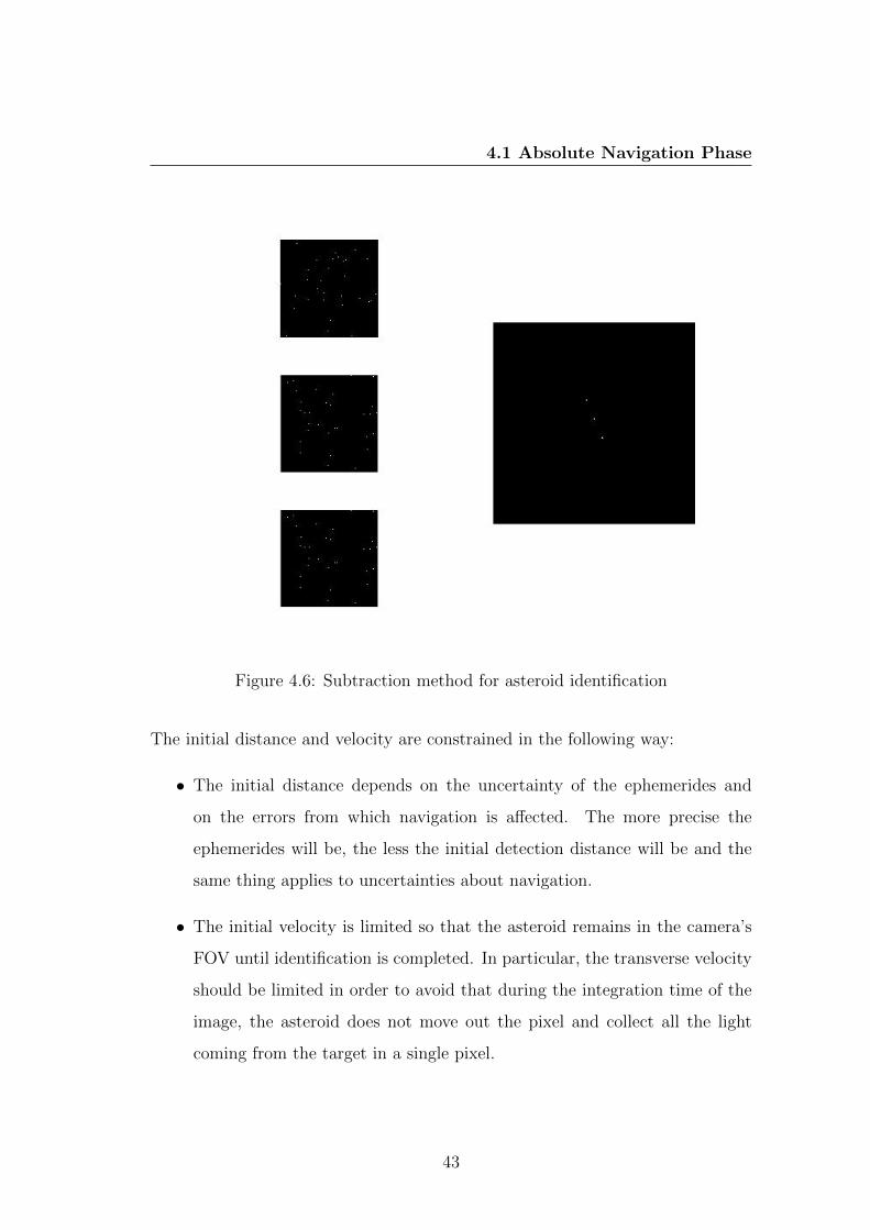
To identify the asteroid a series of images will be taken, as shown in Figure 4.6.
These images will then be processed to isolate the asteroid from the stars in the
background. These images will be subtracted one from another and the trajectory
of the spacecraft will be determined.
42
4.1 Absolute Navigation Phase
Figure 4.6: Subtraction method for asteroid identification
The initial distance and velocity are constrained in the following way:
• The initial distance depends on the uncertainty of the ephemerides and
on the errors from which navigation is affected. The more precise the
ephemerides will be, the less the initial detection distance will be and the
same thing applies to uncertainties about navigation.
• The initial velocity is limited so that the asteroid remains in the camera’s
FOV until identification is completed. In particular, the transverse velocity
should be limited in order to avoid that during the integration time of the
image, the asteroid does not move out the pixel and collect all the light
coming from the target in a single pixel.
43
4.1 Absolute Navigation Phase
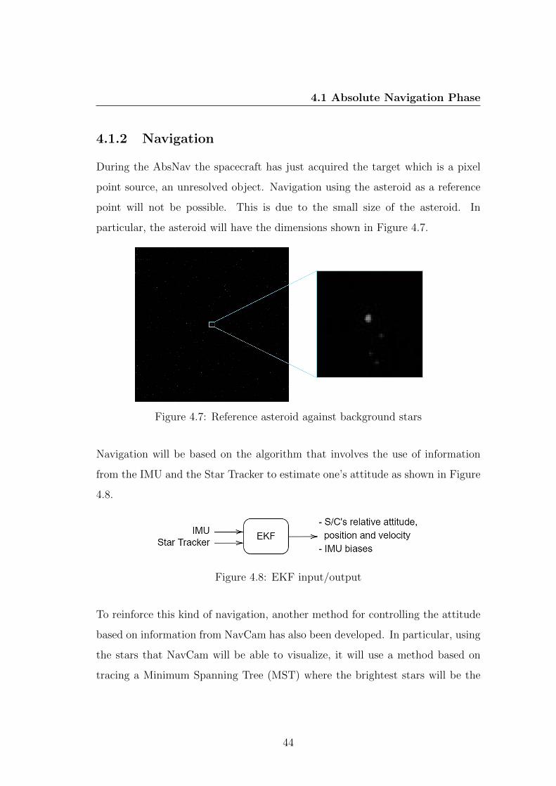
4.1.2 Navigation
During the AbsNav the spacecraft has just acquired the target which is a pixel
point source, an unresolved object. Navigation using the asteroid as a reference
point will not be possible. This is due to the small size of the asteroid. In
particular, the asteroid will have the dimensions shown in Figure 4.7.
Figure 4.7: Reference asteroid against background stars
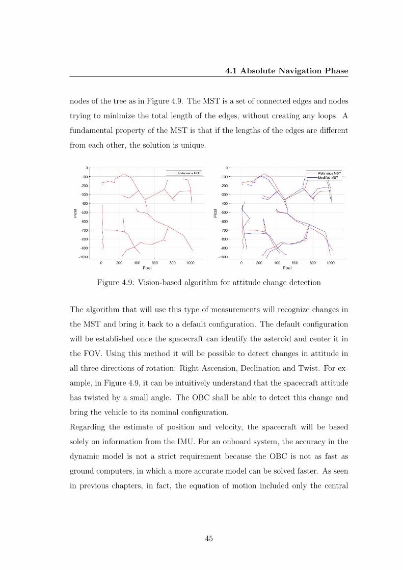
Navigation will be based on the algorithm that involves the use of information
from the IMU and the Star Tracker to estimate one’s attitude as shown in Figure
4.8.
Figure 4.8: EKF input/output
To reinforce this kind of navigation, another method for controlling the attitude
based on information from NavCam has also been developed. In particular, using
the stars that NavCam will be able to visualize, it will use a method based on
tracing a Minimum Spanning Tree (MST) where the brightest stars will be the
44
4.1 Absolute Navigation Phase
nodes of the tree as in Figure 4.9. The MST is a set of connected edges and nodes
trying to minimize the total length of the edges, without creating any loops. A
fundamental property of the MST is that if the lengths of the edges are different
from each other, the solution is unique.
Figure 4.9: Vision-based algorithm for attitude change detection
The algorithm that will use this type of measurements will recognize changes in
the MST and bring it back to a default configuration. The default configuration
will be established once the spacecraft can identify the asteroid and center it in
the FOV. Using this method it will be possible to detect changes in attitude in
all three directions of rotation: Right Ascension, Declination and Twist. For ex-
ample, in Figure 4.9, it can be intuitively understand that the spacecraft attitude
has twisted by a small angle. The OBC shall be able to detect this change and
bring the vehicle to its nominal configuration.
Regarding the estimate of position and velocity, the spacecraft will be based
solely on information from the IMU. For an onboard system, the accuracy in the
dynamic model is not a strict requirement because the OBC is not as fast as
ground computers, in which a more accurate model can be solved faster. As seen
in previous chapters, in fact, the equation of motion included only the central
45
4.1 Absolute Navigation Phase
body gravitational acceleration, the third body point mass gravitational acceler-
ation (Jupiter) and a simple model for the SRP. The onboard thruster activity is
registered by the IMU and included in the integration process.
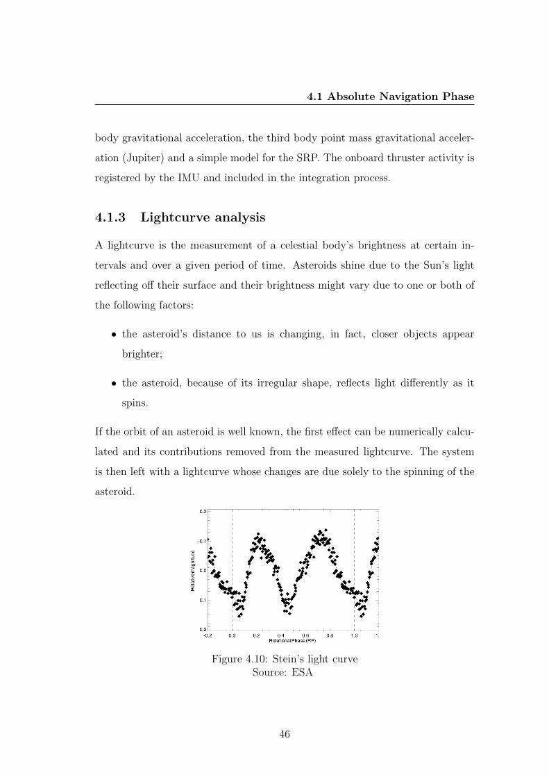
4.1.3 Lightcurve analysis
A lightcurve is the measurement of a celestial body’s brightness at certain in-
tervals and over a given period of time. Asteroids shine due to the Sun’s light
reflecting off their surface and their brightness might vary due to one or both of
the following factors:
• the asteroid’s distance to us is changing, in fact, closer objects appear
brighter;
• the asteroid, because of its irregular shape, reflects light differently as it
spins.
If the orbit of an asteroid is well known, the first effect can be numerically calcu-
lated and its contributions removed from the measured lightcurve. The system
is then left with a lightcurve whose changes are due solely to the spinning of the
asteroid.
Figure 4.10: Stein’s light curveSource: ESA
46
4.1 Absolute Navigation Phase
As has been seen in the State of Art the value of the rotation period of the
asteroid measured from the ground is very close to the real one. Therefore, the
lightcurve will be used initially to verify that the asteroid being targeted is the
correct one. Subsequently, this value will be refined with further measurements
of the lightcurve.
4.1.4 Summary
In this section we discussed:
• how to identify the asteroid against the background stars, dividing the FOV
into parts to be analyzed more carefully. In addition, a method based on
image subtraction for identification has been suggested;
• how to navigate in these conditions where navigation relative to the asteroid
is not possible due to its small size in the image plane;
• how it is necessary to begin to analyze the lightcurve in order to begin to
refine the value of the rotation period estimated through ground observa-
tions.
Table 4.5 summarizes the known properties at the end of the AbsNav phase.
Chemical Composition (estimate)Angular velocitySize (estimate)
Center of BrightnessCentroid3D Model
Center of MassInclination rotation axis
Landmarks
Table 4.5: List of known and unknown properties of the asteroid at the end ofAbsNav
47
4.2 Relative Navigation Phase - Part 1
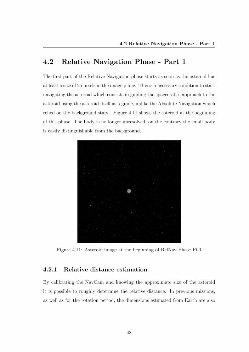
4.2 Relative Navigation Phase - Part 1
The first part of the Relative Navigation phase starts as soon as the asteroid has
at least a size of 25 pixels in the image plane. This is a necessary condition to start
navigating the asteroid which consists in guiding the spacecraft’s approach to the
asteroid using the asteroid itself as a guide, unlike the Absolute Navigation which
relied on the background stars . Figure 4.11 shows the asteroid at the beginning
of this phase. The body is no longer unresolved, on the contrary the small body
is easily distinguishable from the background.
Figure 4.11: Asteroid image at the beginning of RelNav Phase Pt.1
4.2.1 Relative distance estimation
By calibrating the NavCam and knowing the approximate size of the asteroid
it is possible to roughly determine the relative distance. In previous missions,
as well as for the rotation period, the dimensions estimated from Earth are also
48
4.2 Relative Navigation Phase - Part 1
quite close to the real ones [32]. The asteroid size error will determine when the
second part of Relative Navigation phase begins as discussed in the 4.3 section.
Equation 4.1 gives another information: the size of the object on the focal plane
and the distance are inversely proportional. This relation can be exploited to
track the approximate relative distance
dnpx = d25px25
npx
(4.2)
where dnpx is the distance when the asteroid fills a certain amount of pixel, d25px
is the distance computed when the asteroid has 25-pixel dimension on the focal
plane, npx is the number of pixels that the asteroid fills in a certain moment.
The amount of stars on the CCD is less, because of the increased apparent bright-
ness of the asteroid and the subsequent decrease of the exposure time needed to
avoid the image from saturating.
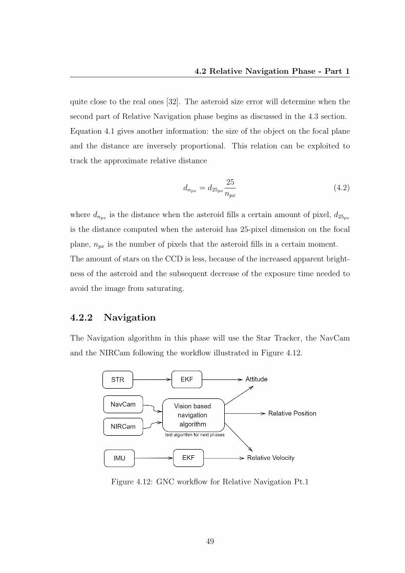
4.2.2 Navigation
The Navigation algorithm in this phase will use the Star Tracker, the NavCam
and the NIRCam following the workflow illustrated in Figure 4.12.
Figure 4.12: GNC workflow for Relative Navigation Pt.1
49
4.2 Relative Navigation Phase - Part 1
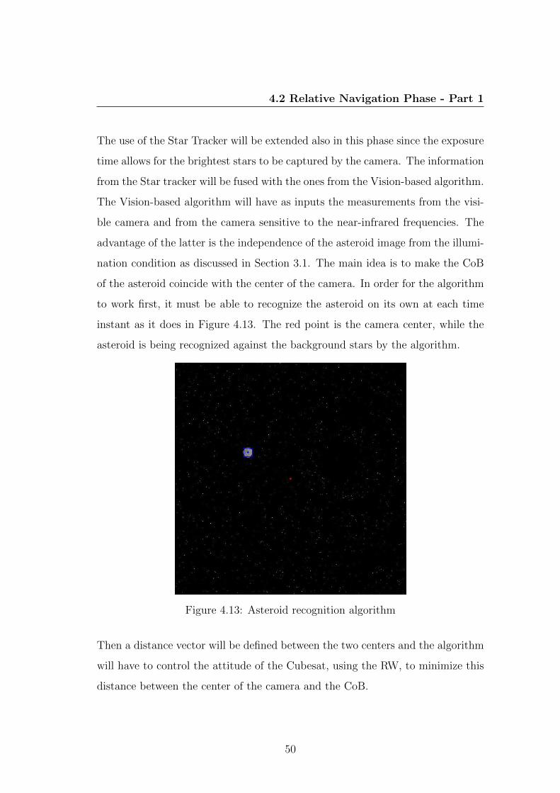
The use of the Star Tracker will be extended also in this phase since the exposure
time allows for the brightest stars to be captured by the camera. The information
from the Star tracker will be fused with the ones from the Vision-based algorithm.
The Vision-based algorithm will have as inputs the measurements from the visi-
ble camera and from the camera sensitive to the near-infrared frequencies. The
advantage of the latter is the independence of the asteroid image from the illumi-
nation condition as discussed in Section 3.1. The main idea is to make the CoB
of the asteroid coincide with the center of the camera. In order for the algorithm
to work first, it must be able to recognize the asteroid on its own at each time
instant as it does in Figure 4.13. The red point is the camera center, while the
asteroid is being recognized against the background stars by the algorithm.
Figure 4.13: Asteroid recognition algorithm
Then a distance vector will be defined between the two centers and the algorithm
will have to control the attitude of the Cubesat, using the RW, to minimize this
distance between the center of the camera and the CoB.
50
4.2 Relative Navigation Phase - Part 1
It is known that navigation referred to CoB can give degraded results, obtaining
a poor quality pointing towards the asteroid, in which the deviation from CoM
can be relevant. As can be seen from Figure 4.11 in these early stages the di-
mensions of the asteroid are still small, so the error between CoM and CoB are
small. Therefore navigation using the latter as a reference maintains an excellent
performance.
4.2.3 Debris Analysis
As the spacecraft approaches the asteroid it should start an analysis of the sur-
rounding environment to detect orbiting objects around the asteroid, in case of
binary systems, or for dust orbiting around that might endanger the spacecraft.
In the case of small bodies, the gravitational force is not strong enough to retain
any object in its surroundings. So no analysis will be carried out regarding this
issue.
4.2.4 Summary
In this section we discussed:
• how to estimate the relative distance by using information from ground-
based observation;
• how the navigation algorithm changes from the previous phase. In particu-
lar, it has been discussed how the navigation referred to the CoB is suitable
for this phase.
Table 4.6 summarizes the known properties at the end of the first part of the
RelNav phase.
51
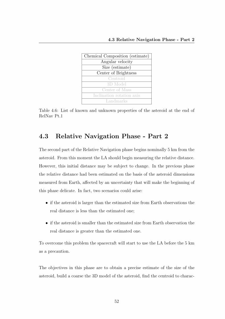
4.3 Relative Navigation Phase - Part 2
Chemical Composition (estimate)Angular velocitySize (estimate)
Center of BrightnessCentroid3D Model
Center of MassInclination rotation axis
Landmarks
Table 4.6: List of known and unknown properties of the asteroid at the end ofRelNav Pt.1
4.3 Relative Navigation Phase - Part 2
The second part of the Relative Navigation phase begins nominally 5 km from the
asteroid. From this moment the LA should begin measuring the relative distance.
However, this initial distance may be subject to change. In the previous phase
the relative distance had been estimated on the basis of the asteroid dimensions
measured from Earth, affected by an uncertainty that will make the beginning of
this phase delicate. In fact, two scenarios could arise:
• if the asteroid is larger than the estimated size from Earth observations the
real distance is less than the estimated one;
• if the asteroid is smaller than the estimated size from Earth observation the
real distance is greater than the estimated one.
To overcome this problem the spacecraft will start to use the LA before the 5 km
as a precaution.
The objectives in this phase are to obtain a precise estimate of the size of the
asteroid, build a coarse the 3D model of the asteroid, find the centroid to charac-
52
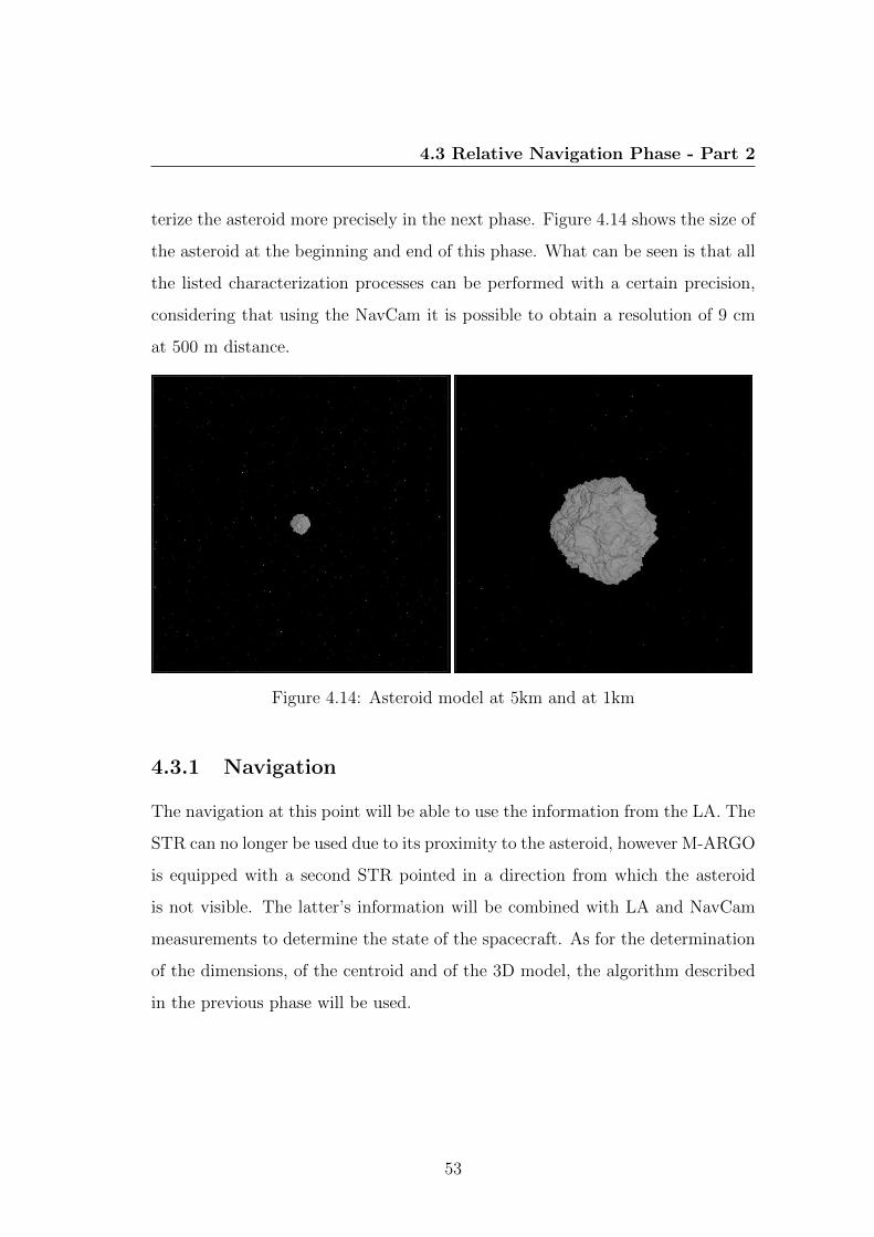
4.3 Relative Navigation Phase - Part 2
terize the asteroid more precisely in the next phase. Figure 4.14 shows the size of
the asteroid at the beginning and end of this phase. What can be seen is that all
the listed characterization processes can be performed with a certain precision,
considering that using the NavCam it is possible to obtain a resolution of 9 cm
at 500 m distance.
Figure 4.14: Asteroid model at 5km and at 1km
4.3.1 Navigation
The navigation at this point will be able to use the information from the LA. The
STR can no longer be used due to its proximity to the asteroid, however M-ARGO
is equipped with a second STR pointed in a direction from which the asteroid
is not visible. The latter’s information will be combined with LA and NavCam
measurements to determine the state of the spacecraft. As for the determination
of the dimensions, of the centroid and of the 3D model, the algorithm described
in the previous phase will be used.
53
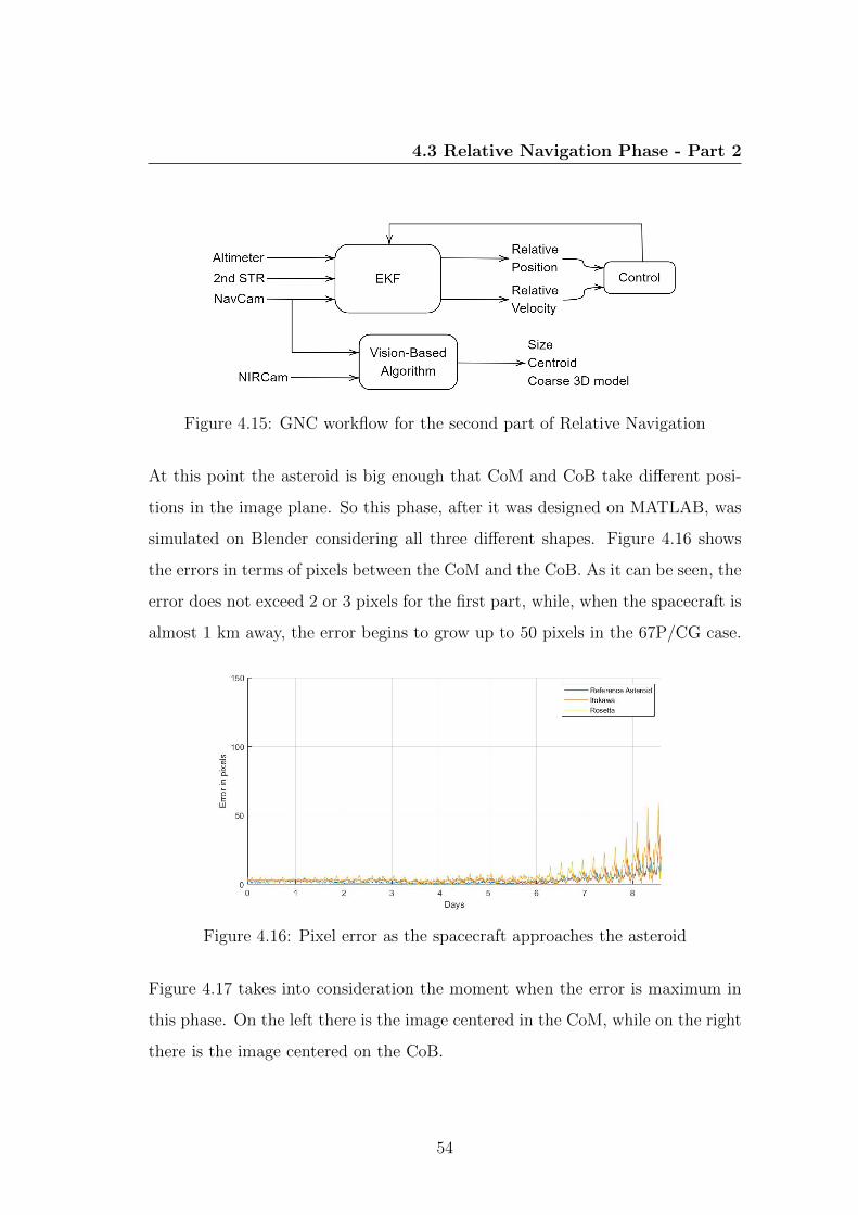
4.3 Relative Navigation Phase - Part 2
Figure 4.15: GNC workflow for the second part of Relative Navigation
At this point the asteroid is big enough that CoM and CoB take different posi-
tions in the image plane. So this phase, after it was designed on MATLAB, was
simulated on Blender considering all three different shapes. Figure 4.16 shows
the errors in terms of pixels between the CoM and the CoB. As it can be seen, the
error does not exceed 2 or 3 pixels for the first part, while, when the spacecraft is
almost 1 km away, the error begins to grow up to 50 pixels in the 67P/CG case.
Figure 4.16: Pixel error as the spacecraft approaches the asteroid
Figure 4.17 takes into consideration the moment when the error is maximum in
this phase. On the left there is the image centered in the CoM, while on the right
there is the image centered on the CoB.
54
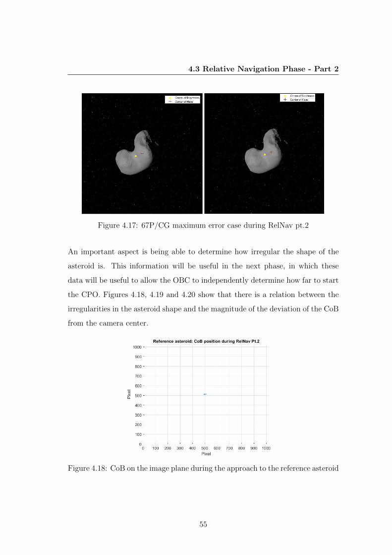
4.3 Relative Navigation Phase - Part 2
Figure 4.17: 67P/CG maximum error case during RelNav pt.2
An important aspect is being able to determine how irregular the shape of the
asteroid is. This information will be useful in the next phase, in which these
data will be useful to allow the OBC to independently determine how far to start
the CPO. Figures 4.18, 4.19 and 4.20 show that there is a relation between the
irregularities in the asteroid shape and the magnitude of the deviation of the CoB
from the camera center.
Figure 4.18: CoB on the image plane during the approach to the reference asteroid
55
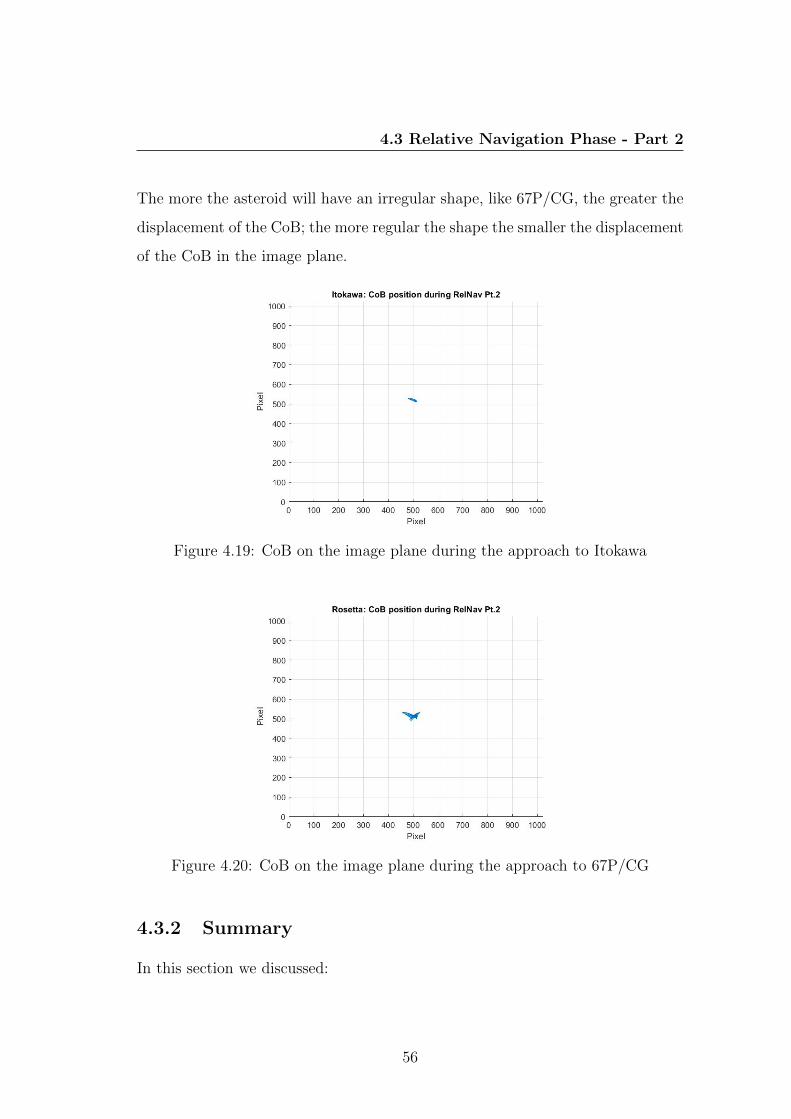
4.3 Relative Navigation Phase - Part 2
The more the asteroid will have an irregular shape, like 67P/CG, the greater the
displacement of the CoB; the more regular the shape the smaller the displacement
of the CoB in the image plane.
Figure 4.19: CoB on the image plane during the approach to Itokawa
Figure 4.20: CoB on the image plane during the approach to 67P/CG
4.3.2 Summary
In this section we discussed:
56
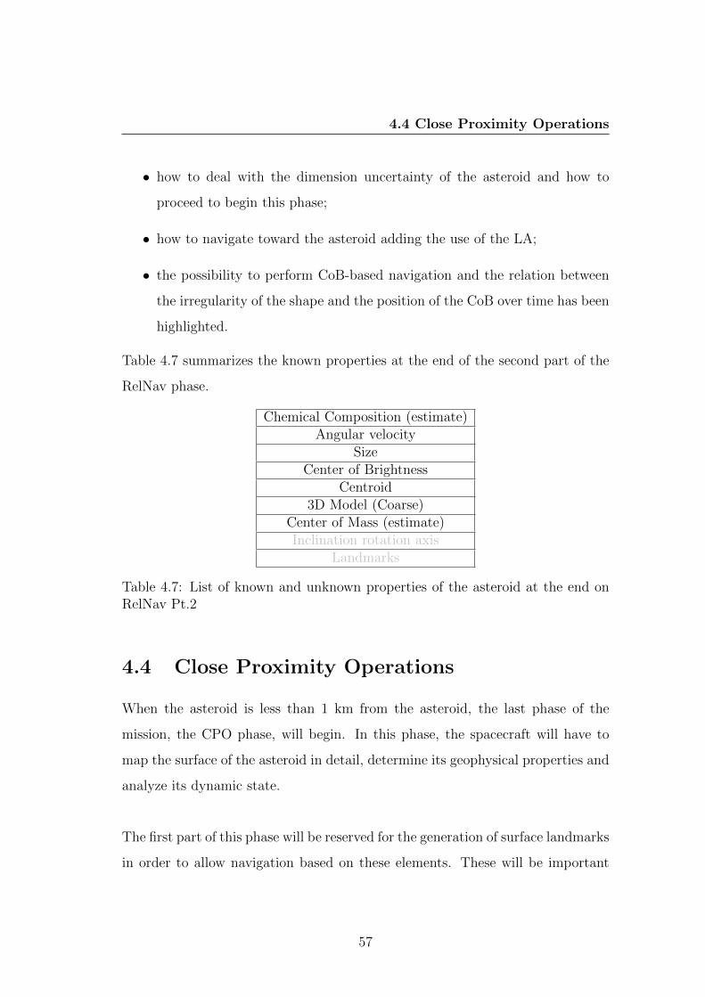
4.4 Close Proximity Operations
• how to deal with the dimension uncertainty of the asteroid and how to
proceed to begin this phase;
• how to navigate toward the asteroid adding the use of the LA;
• the possibility to perform CoB-based navigation and the relation between
the irregularity of the shape and the position of the CoB over time has been
highlighted.
Table 4.7 summarizes the known properties at the end of the second part of the
RelNav phase.
Chemical Composition (estimate)Angular velocity
SizeCenter of Brightness
Centroid3D Model (Coarse)
Center of Mass (estimate)Inclination rotation axis
Landmarks
Table 4.7: List of known and unknown properties of the asteroid at the end onRelNav Pt.2
4.4 Close Proximity Operations
When the asteroid is less than 1 km from the asteroid, the last phase of the
mission, the CPO phase, will begin. In this phase, the spacecraft will have to
map the surface of the asteroid in detail, determine its geophysical properties and
analyze its dynamic state.
The first part of this phase will be reserved for the generation of surface landmarks
in order to allow navigation based on these elements. These will be important
57
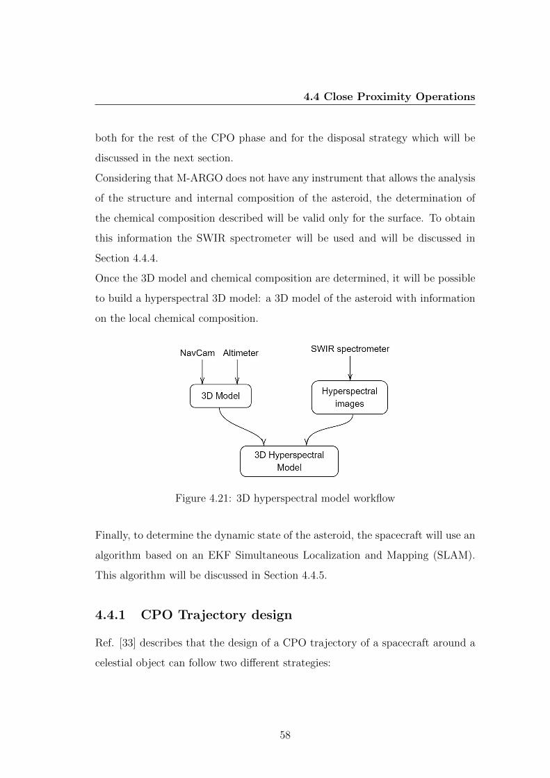
4.4 Close Proximity Operations
both for the rest of the CPO phase and for the disposal strategy which will be
discussed in the next section.
Considering that M-ARGO does not have any instrument that allows the analysis
of the structure and internal composition of the asteroid, the determination of
the chemical composition described will be valid only for the surface. To obtain
this information the SWIR spectrometer will be used and will be discussed in
Section 4.4.4.
Once the 3D model and chemical composition are determined, it will be possible
to build a hyperspectral 3D model: a 3D model of the asteroid with information
on the local chemical composition.
Figure 4.21: 3D hyperspectral model workflow
Finally, to determine the dynamic state of the asteroid, the spacecraft will use an
algorithm based on an EKF Simultaneous Localization and Mapping (SLAM).
This algorithm will be discussed in Section 4.4.5.
4.4.1 CPO Trajectory design
Ref. [33] describes that the design of a CPO trajectory of a spacecraft around a
celestial object can follow two different strategies:
58
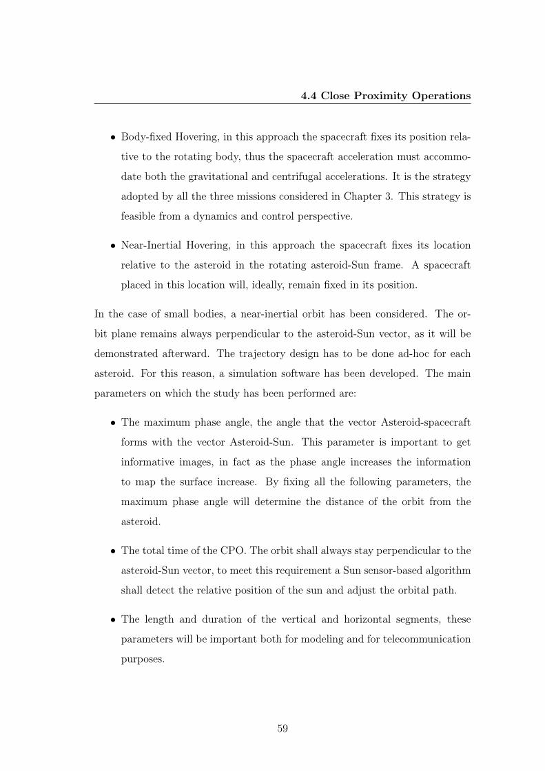
4.4 Close Proximity Operations
• Body-fixed Hovering, in this approach the spacecraft fixes its position rela-
tive to the rotating body, thus the spacecraft acceleration must accommo-
date both the gravitational and centrifugal accelerations. It is the strategy
adopted by all the three missions considered in Chapter 3. This strategy is
feasible from a dynamics and control perspective.
• Near-Inertial Hovering, in this approach the spacecraft fixes its location
relative to the asteroid in the rotating asteroid-Sun frame. A spacecraft
placed in this location will, ideally, remain fixed in its position.
In the case of small bodies, a near-inertial orbit has been considered. The or-
bit plane remains always perpendicular to the asteroid-Sun vector, as it will be
demonstrated afterward. The trajectory design has to be done ad-hoc for each
asteroid. For this reason, a simulation software has been developed. The main
parameters on which the study has been performed are:
• The maximum phase angle, the angle that the vector Asteroid-spacecraft
forms with the vector Asteroid-Sun. This parameter is important to get
informative images, in fact as the phase angle increases the information
to map the surface increase. By fixing all the following parameters, the
maximum phase angle will determine the distance of the orbit from the
asteroid.
• The total time of the CPO. The orbit shall always stay perpendicular to the
asteroid-Sun vector, to meet this requirement a Sun sensor-based algorithm
shall detect the relative position of the sun and adjust the orbital path.
• The length and duration of the vertical and horizontal segments, these
parameters will be important both for modeling and for telecommunication
purposes.
59
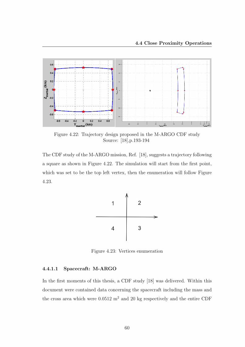
4.4 Close Proximity Operations
Figure 4.22: Trajectory design proposed in the M-ARGO CDF studySource: [18],p.193-194
The CDF study of the M-ARGO mission, Ref. [18], suggests a trajectory following
a square as shown in Figure 4.22. The simulation will start from the first point,
which was set to be the top left vertex, then the enumeration will follow Figure
4.23.
Figure 4.23: Vertices enumeration
4.4.1.1 Spacecraft: M-ARGO
In the first moments of this thesis, a CDF study [18] was delivered. Within this
document were contained data concerning the spacecraft including the mass and
the cross area which were 0.0512 m2 and 20 kg respectively and the entire CDF
60
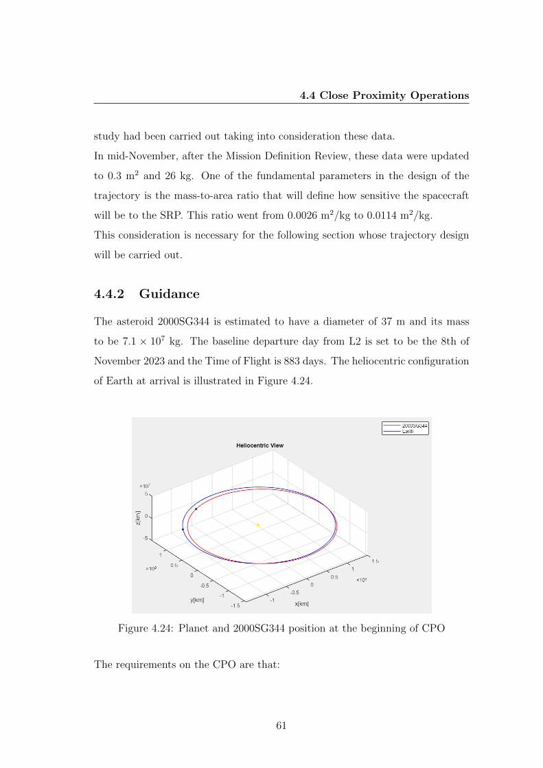
4.4 Close Proximity Operations
study had been carried out taking into consideration these data.
In mid-November, after the Mission Definition Review, these data were updated
to 0.3 m2 and 26 kg. One of the fundamental parameters in the design of the
trajectory is the mass-to-area ratio that will define how sensitive the spacecraft
will be to the SRP. This ratio went from 0.0026 m2/kg to 0.0114 m2/kg.
This consideration is necessary for the following section whose trajectory design
will be carried out.
4.4.2 Guidance
The asteroid 2000SG344 is estimated to have a diameter of 37 m and its mass
to be 7.1 × 10⁷ kg. The baseline departure day from L2 is set to be the 8th of
November 2023 and the Time of Flight is 883 days. The heliocentric configuration
of Earth at arrival is illustrated in Figure 4.24.
Figure 4.24: Planet and 2000SG344 position at the beginning of CPO
The requirements on the CPO are that:
61
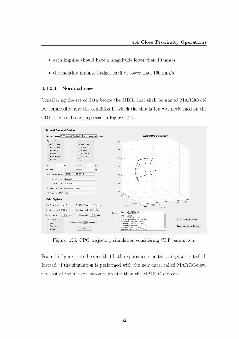
4.4 Close Proximity Operations
• each impulse should have a magnitude lower than 10 mm/s;
• the monthly impulse budget shall be lower than 100 mm/s
4.4.2.1 Nominal case
Considering the set of data before the MDR, that shall be named MARGO-old
for commodity, and the condition in which the simulation was performed on the
CDF, the results are reported in Figure 4.25.
Figure 4.25: CPO trajectory simulation considering CDF parameters
From the figure it can be seen that both requirements on the budget are satisfied.
Instead, if the simulation is performed with the new data, called MARGO-new,
the cost of the mission becomes greater than the MARGO-old case.
62
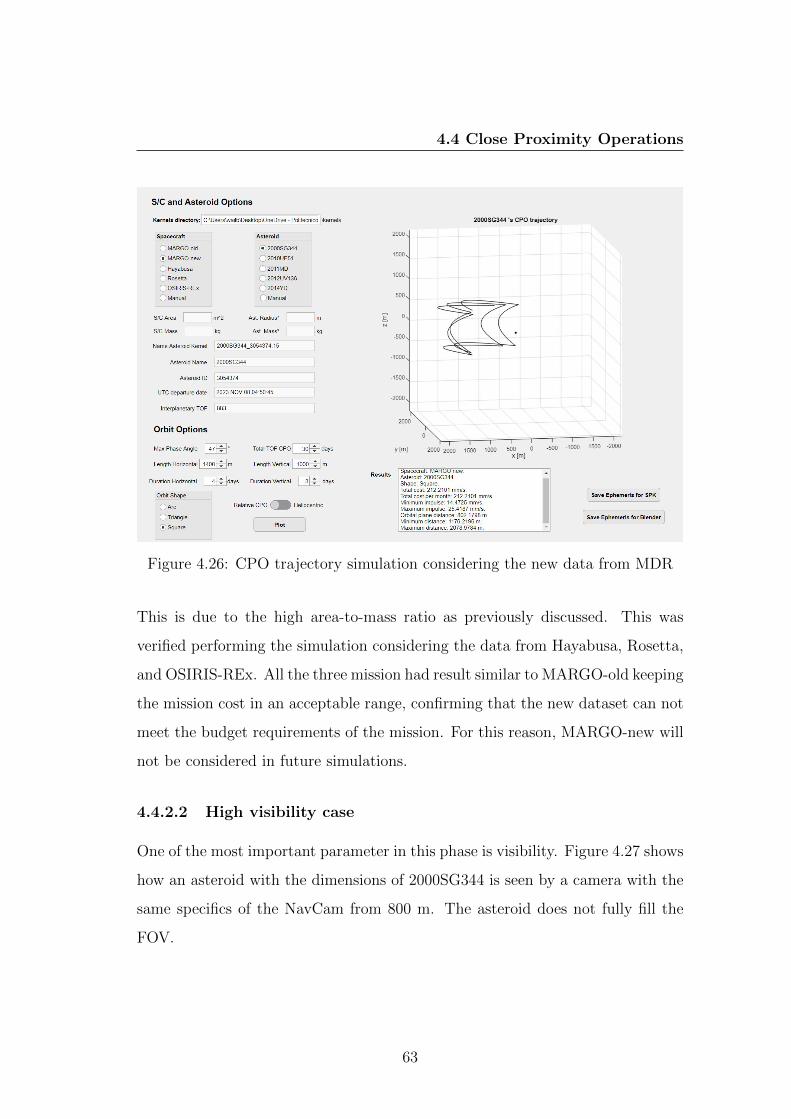
4.4 Close Proximity Operations
Figure 4.26: CPO trajectory simulation considering the new data from MDR
This is due to the high area-to-mass ratio as previously discussed. This was
verified performing the simulation considering the data from Hayabusa, Rosetta,
and OSIRIS-REx. All the three mission had result similar to MARGO-old keeping
the mission cost in an acceptable range, confirming that the new dataset can not
meet the budget requirements of the mission. For this reason, MARGO-new will
not be considered in future simulations.
4.4.2.2 High visibility case
One of the most important parameter in this phase is visibility. Figure 4.27 shows
how an asteroid with the dimensions of 2000SG344 is seen by a camera with the
same specifics of the NavCam from 800 m. The asteroid does not fully fill the
FOV.
63
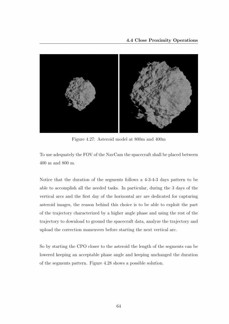
4.4 Close Proximity Operations
Figure 4.27: Asteroid model at 800m and 400m
To use adequately the FOV of the NavCam the spacecraft shall be placed between
400 m and 800 m.
Notice that the duration of the segments follows a 4-3-4-3 days pattern to be
able to accomplish all the needed tasks. In particular, during the 3 days of the
vertical arcs and the first day of the horizontal arc are dedicated for capturing
asteroid images, the reason behind this choice is to be able to exploit the part
of the trajectory characterized by a higher angle phase and using the rest of the
trajectory to download to ground the spacecraft data, analyze the trajectory and
upload the correction maneuvers before starting the next vertical arc.
So by starting the CPO closer to the asteroid the length of the segments can be
lowered keeping an acceptable phase angle and keeping unchanged the duration
of the segments pattern. Figure 4.28 shows a possible solution.
64
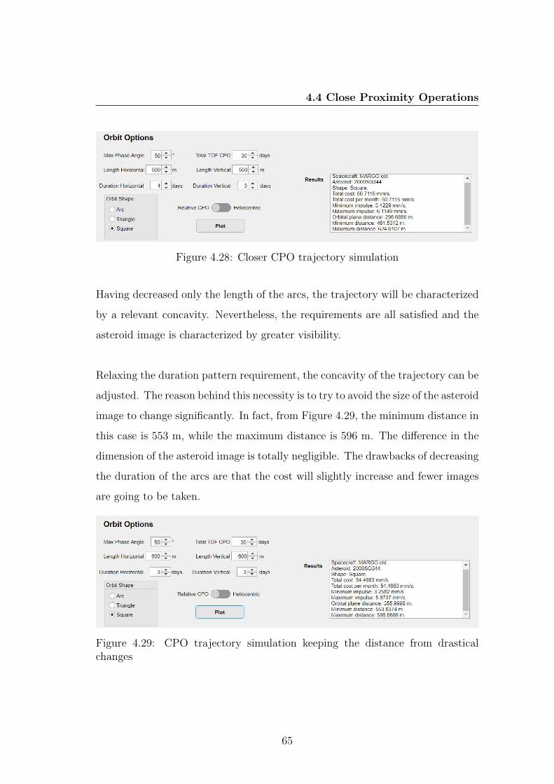
4.4 Close Proximity Operations
Figure 4.28: Closer CPO trajectory simulation
Having decreased only the length of the arcs, the trajectory will be characterized
by a relevant concavity. Nevertheless, the requirements are all satisfied and the
asteroid image is characterized by greater visibility.
Relaxing the duration pattern requirement, the concavity of the trajectory can be
adjusted. The reason behind this necessity is to try to avoid the size of the asteroid
image to change significantly. In fact, from Figure 4.29, the minimum distance in
this case is 553 m, while the maximum distance is 596 m. The difference in the
dimension of the asteroid image is totally negligible. The drawbacks of decreasing
the duration of the arcs are that the cost will slightly increase and fewer images
are going to be taken.
Figure 4.29: CPO trajectory simulation keeping the distance from drasticalchanges
65
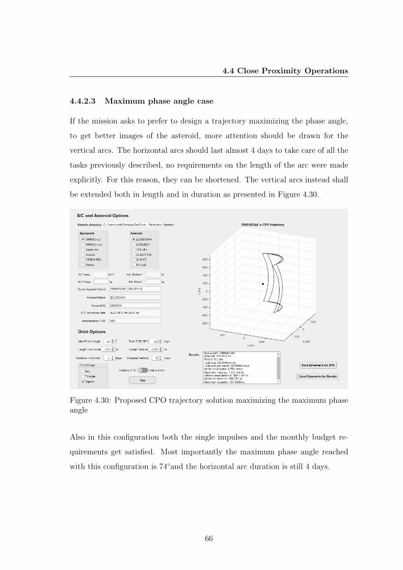
4.4 Close Proximity Operations
4.4.2.3 Maximum phase angle case
If the mission asks to prefer to design a trajectory maximizing the phase angle,
to get better images of the asteroid, more attention should be drawn for the
vertical arcs. The horizontal arcs should last almost 4 days to take care of all the
tasks previously described, no requirements on the length of the arc were made
explicitly. For this reason, they can be shortened. The vertical arcs instead shall
be extended both in length and in duration as presented in Figure 4.30.
Figure 4.30: Proposed CPO trajectory solution maximizing the maximum phaseangle
Also in this configuration both the single impulses and the monthly budget re-
quirements get satisfied. Most importantly the maximum phase angle reached
with this configuration is 74◦and the horizontal arc duration is still 4 days.
66
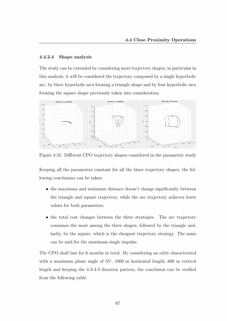
4.4 Close Proximity Operations
4.4.2.4 Shape analysis
The study can be extended by considering more trajectory shapes, in particular in
this analysis, it will be considered the trajectory composed by a single hyperbolic
arc, by three hyperbolic arcs forming a triangle shape and by four hyperbolic arcs
forming the square shape previously taken into consideration.
Figure 4.31: Different CPO trajectory shapes considered in the parametric study
Keeping all the parameters constant for all the three trajectory shapes, the fol-
lowing conclusions can be taken:
• the maximum and minimum distance doesn’t change significantly between
the triangle and square trajectory, while the arc trajectory achieves lower
values for both parameters;
• the total cost changes between the three strategies. The arc trajectory
consumes the most among the three shapes, followed by the triangle and,
lastly, by the square, which is the cheapest trajectory strategy. The same
can be said for the maximum single impulse.
The CPO shall last for 6 months in total. By considering an orbit characterized
with a maximum phase angle of 55◦, 1000 m horizontal length, 600 m vertical
length and keeping the 4-3-4-3 duration pattern, the conclusion can be verified
from the following table.
67
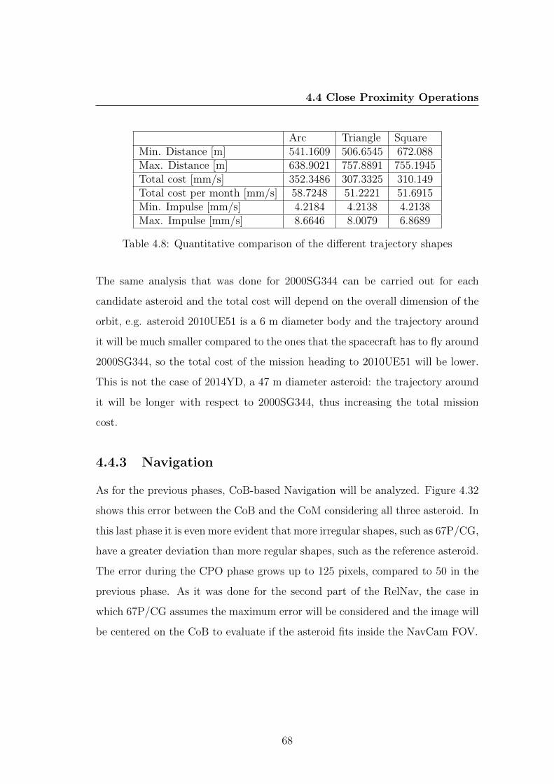
4.4 Close Proximity Operations
Arc Triangle SquareMin. Distance [m] 541.1609 506.6545 672.088Max. Distance [m] 638.9021 757.8891 755.1945Total cost [mm/s] 352.3486 307.3325 310.149Total cost per month [mm/s] 58.7248 51.2221 51.6915Min. Impulse [mm/s] 4.2184 4.2138 4.2138Max. Impulse [mm/s] 8.6646 8.0079 6.8689
Table 4.8: Quantitative comparison of the different trajectory shapes
The same analysis that was done for 2000SG344 can be carried out for each
candidate asteroid and the total cost will depend on the overall dimension of the
orbit, e.g. asteroid 2010UE51 is a 6 m diameter body and the trajectory around
it will be much smaller compared to the ones that the spacecraft has to fly around
2000SG344, so the total cost of the mission heading to 2010UE51 will be lower.
This is not the case of 2014YD, a 47 m diameter asteroid: the trajectory around
it will be longer with respect to 2000SG344, thus increasing the total mission
cost.
4.4.3 Navigation
As for the previous phases, CoB-based Navigation will be analyzed. Figure 4.32
shows this error between the CoB and the CoM considering all three asteroid. In
this last phase it is even more evident that more irregular shapes, such as 67P/CG,
have a greater deviation than more regular shapes, such as the reference asteroid.
The error during the CPO phase grows up to 125 pixels, compared to 50 in the
previous phase. As it was done for the second part of the RelNav, the case in
which 67P/CG assumes the maximum error will be considered and the image will
be centered on the CoB to evaluate if the asteroid fits inside the NavCam FOV.
68
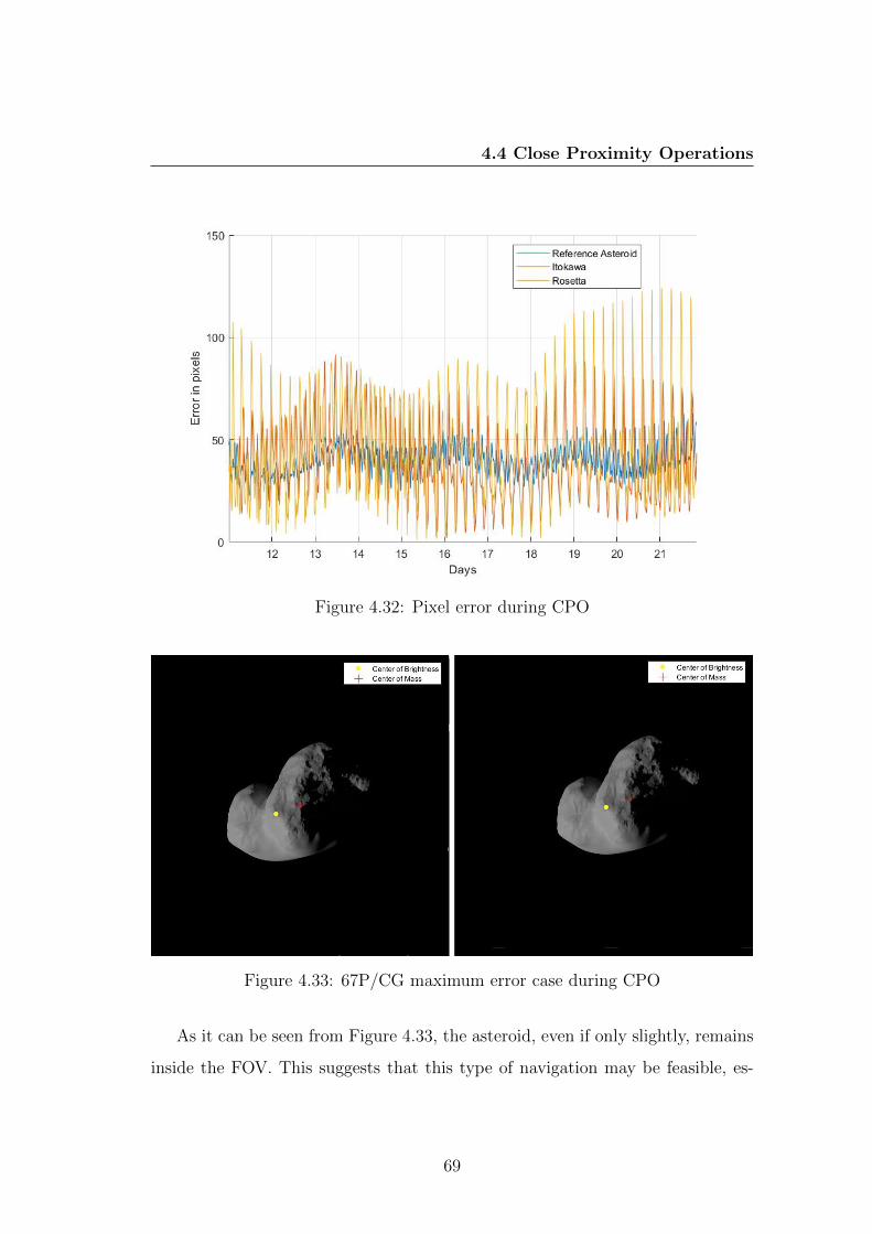
4.4 Close Proximity Operations
Figure 4.32: Pixel error during CPO
Figure 4.33: 67P/CG maximum error case during CPO
As it can be seen from Figure 4.33, the asteroid, even if only slightly, remains
inside the FOV. This suggests that this type of navigation may be feasible, es-
69
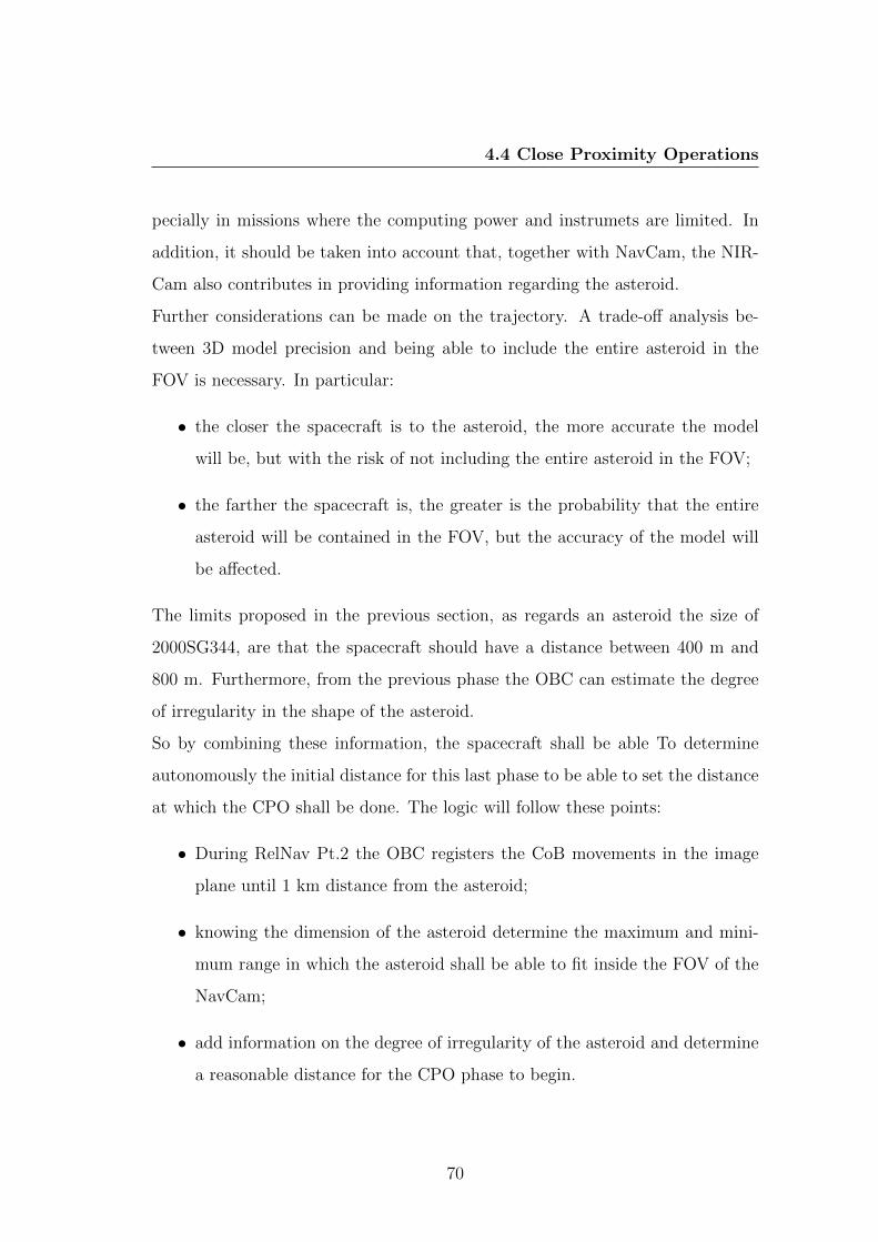
4.4 Close Proximity Operations
pecially in missions where the computing power and instrumets are limited. In
addition, it should be taken into account that, together with NavCam, the NIR-
Cam also contributes in providing information regarding the asteroid.
Further considerations can be made on the trajectory. A trade-off analysis be-
tween 3D model precision and being able to include the entire asteroid in the
FOV is necessary. In particular:
• the closer the spacecraft is to the asteroid, the more accurate the model
will be, but with the risk of not including the entire asteroid in the FOV;
• the farther the spacecraft is, the greater is the probability that the entire
asteroid will be contained in the FOV, but the accuracy of the model will
be affected.
The limits proposed in the previous section, as regards an asteroid the size of
2000SG344, are that the spacecraft should have a distance between 400 m and
800 m. Furthermore, from the previous phase the OBC can estimate the degree
of irregularity in the shape of the asteroid.
So by combining these information, the spacecraft shall be able To determine
autonomously the initial distance for this last phase to be able to set the distance
at which the CPO shall be done. The logic will follow these points:
• During RelNav Pt.2 the OBC registers the CoB movements in the image
plane until 1 km distance from the asteroid;
• knowing the dimension of the asteroid determine the maximum and mini-
mum range in which the asteroid shall be able to fit inside the FOV of the
NavCam;
• add information on the degree of irregularity of the asteroid and determine
a reasonable distance for the CPO phase to begin.
70
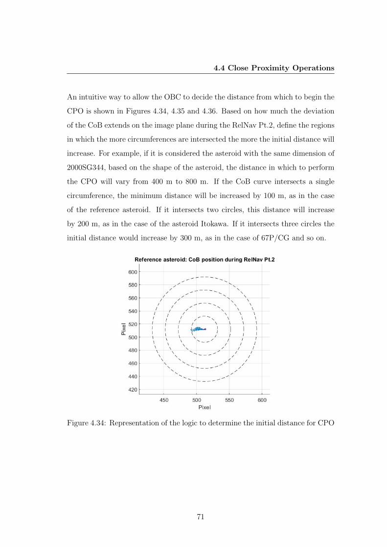
4.4 Close Proximity Operations
An intuitive way to allow the OBC to decide the distance from which to begin the
CPO is shown in Figures 4.34, 4.35 and 4.36. Based on how much the deviation
of the CoB extends on the image plane during the RelNav Pt.2, define the regions
in which the more circumferences are intersected the more the initial distance will
increase. For example, if it is considered the asteroid with the same dimension of
2000SG344, based on the shape of the asteroid, the distance in which to perform
the CPO will vary from 400 m to 800 m. If the CoB curve intersects a single
circumference, the minimum distance will be increased by 100 m, as in the case
of the reference asteroid. If it intersects two circles, this distance will increase
by 200 m, as in the case of the asteroid Itokawa. If it intersects three circles the
initial distance would increase by 300 m, as in the case of 67P/CG and so on.
Figure 4.34: Representation of the logic to determine the initial distance for CPO
71
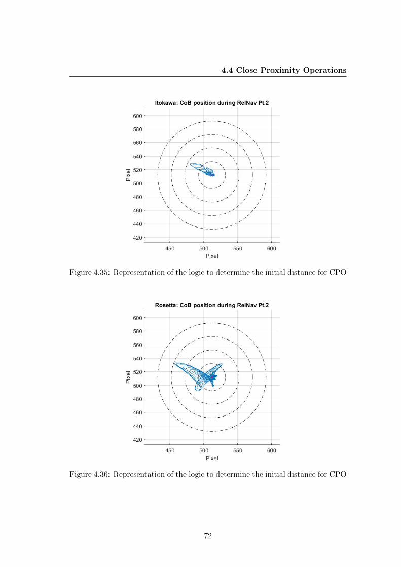
4.4 Close Proximity Operations
Figure 4.35: Representation of the logic to determine the initial distance for CPO
Figure 4.36: Representation of the logic to determine the initial distance for CPO
72
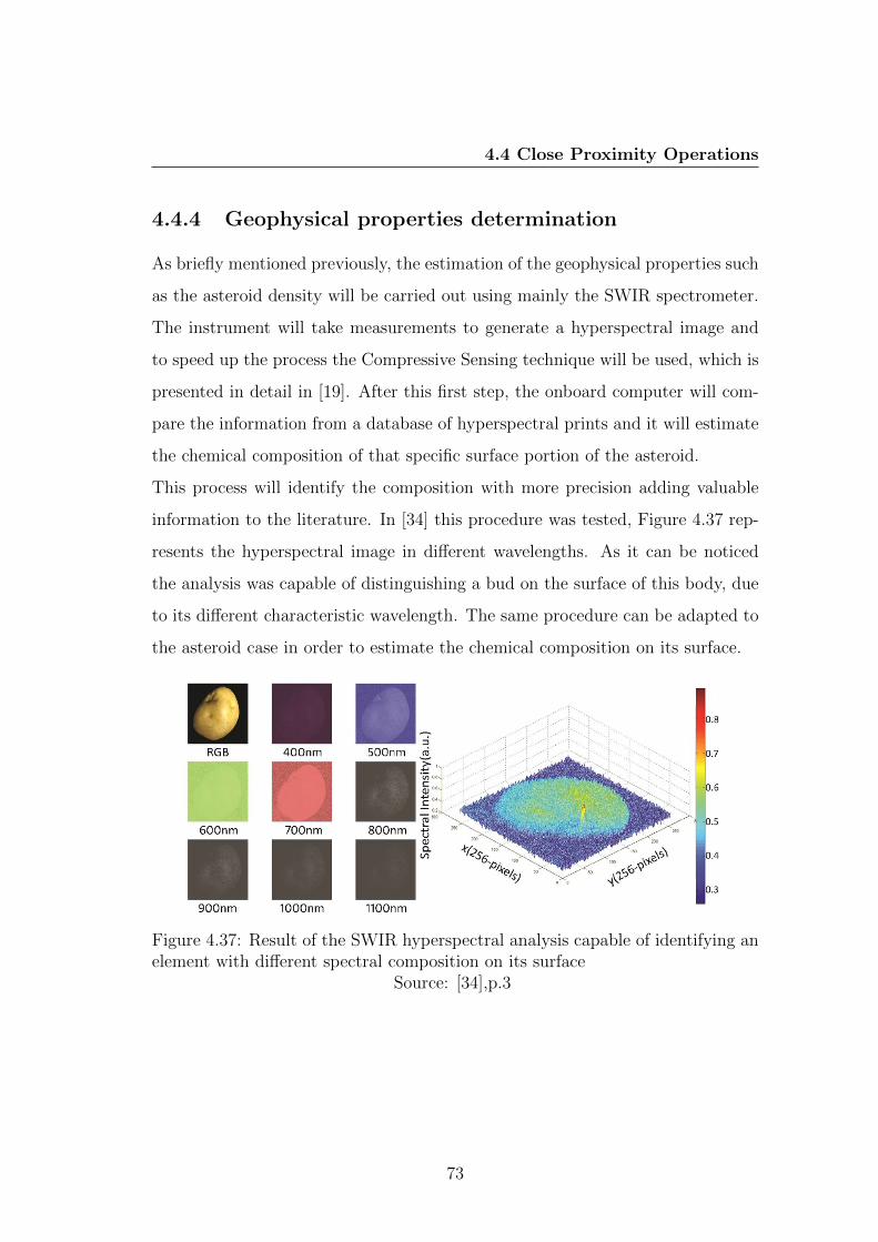
4.4 Close Proximity Operations
4.4.4 Geophysical properties determination
As briefly mentioned previously, the estimation of the geophysical properties such
as the asteroid density will be carried out using mainly the SWIR spectrometer.
The instrument will take measurements to generate a hyperspectral image and
to speed up the process the Compressive Sensing technique will be used, which is
presented in detail in [19]. After this first step, the onboard computer will com-
pare the information from a database of hyperspectral prints and it will estimate
the chemical composition of that specific surface portion of the asteroid.
This process will identify the composition with more precision adding valuable
information to the literature. In [34] this procedure was tested, Figure 4.37 rep-
resents the hyperspectral image in different wavelengths. As it can be noticed
the analysis was capable of distinguishing a bud on the surface of this body, due
to its different characteristic wavelength. The same procedure can be adapted to
the asteroid case in order to estimate the chemical composition on its surface.
Figure 4.37: Result of the SWIR hyperspectral analysis capable of identifying anelement with different spectral composition on its surface
Source: [34],p.3
73
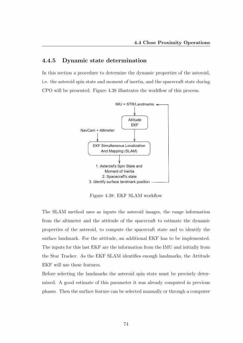
4.4 Close Proximity Operations
4.4.5 Dynamic state determination
In this section a procedure to determine the dynamic properties of the asteroid,
i.e. the asteroid spin state and moment of inertia, and the spacecraft state during
CPO will be presented. Figure 4.38 illustrates the workflow of this process.
Figure 4.38: EKF SLAM workflow
The SLAM method uses as inputs the asteroid images, the range information
from the altimeter and the attitude of the spacecraft to estimate the dynamic
properties of the asteroid, to compute the spacecraft state and to identify the
surface landmark. For the attitude, an additional EKF has to be implemented.
The inputs for this last EKF are the information from the IMU and initially from
the Star Tracker. As the EKF SLAM identifies enough landmarks, the Attitude
EKF will use these features.
Before selecting the landmarks the asteroid spin state must be precisely deter-
mined. A good estimate of this parameter it was already computed in previous
phases. Then the surface feature can be selected manually or through a computer
74
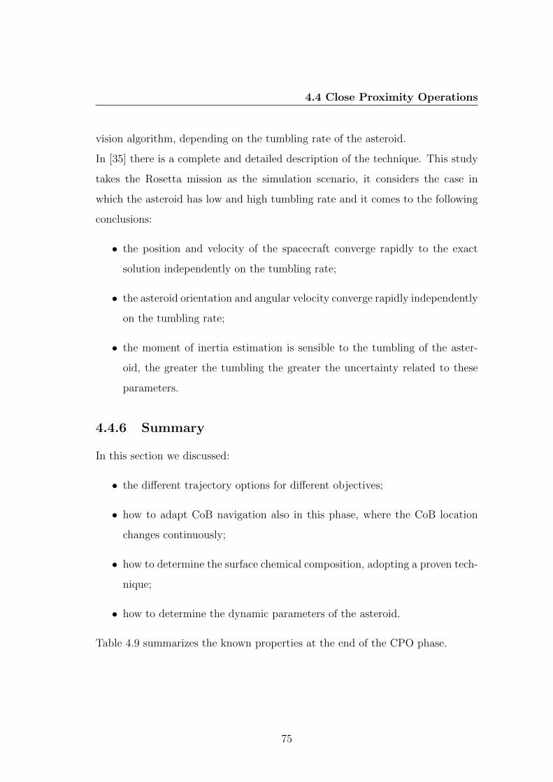
4.4 Close Proximity Operations
vision algorithm, depending on the tumbling rate of the asteroid.
In [35] there is a complete and detailed description of the technique. This study
takes the Rosetta mission as the simulation scenario, it considers the case in
which the asteroid has low and high tumbling rate and it comes to the following
conclusions:
• the position and velocity of the spacecraft converge rapidly to the exact
solution independently on the tumbling rate;
• the asteroid orientation and angular velocity converge rapidly independently
on the tumbling rate;
• the moment of inertia estimation is sensible to the tumbling of the aster-
oid, the greater the tumbling the greater the uncertainty related to these
parameters.
4.4.6 Summary
In this section we discussed:
• the different trajectory options for different objectives;
• how to adapt CoB navigation also in this phase, where the CoB location
changes continuously;
• how to determine the surface chemical composition, adopting a proven tech-
nique;
• how to determine the dynamic parameters of the asteroid.
Table 4.9 summarizes the known properties at the end of the CPO phase.
75
4.5 Disposal strategy: Landing
Chemical CompositionAngular velocity
SizeCenter of Brightness
Centroid3D Model
Center of MassInclination rotation axis
Landmarks
Table 4.9: List of known and unknown properties of the asteroid at the end onCPO
4.5 Disposal strategy: Landing
At the end of mission, the spacecraft shall be disposed appropriately, by either
attempting a landing on the target asteroid or allowing the spacecraft to drift
into a heliocentric graveyard orbit. The spacecraft is not designed to be able
to land, nevertheless by exploiting the information gathered, the remaining EPS
and RCS propellant a landing procedure is here proposed.
The hypotheses on which the maneuver is based on are that the nutation effect is
neglected in a short time interval, as it can be confirmed in the Itokawa asteroid
which nutation was 0,128 deg/year from Ref. [36]. This hypothesis will guarantee
that the pole position can be considered fixed. Also, the radiometric link with
the ground station shall be available.
• Once the 3D model and the information on its surface feature is available,
the Ground Station defines a series of maneuvers to get closer to the pole
lit by the Sun.
• Once the spacecraft is located onto the pole it shall map in detail the surface
of the pole to identify candidate landing spots.
76
4.6 Error Sources
• To guide the spacecraft the NavCam and LA shall be active.
• Initiate the spin of the spacecraft with the RCS. Following the indication
given on [18], the RCS can spin the spacecraft up to 1.5 rad/s in 10 min.
• Facing the NavCam toward the surface the EPS will be able to fire to get
the spacecraft closer to the surface of the asteroid in a controlled way.
• While going toward the asteroid the position shall be corrected and the
velocity precisely controlled down to a few mm/s.
• The landing shall be verified using both optical instrument and LA.
4.6 Error Sources
Here are briefly listed the possible error sources that could affect optical naviga-
tion.
• The inertial direction of the Line of Sight vector, if the stars are not in the
camera FOV then the inertial pointing of the camera will be affected by a
large error that must be accounted for and must be estimated in the filter.
• Errors in the location of the target body or the landmark on its surface will
corrupt the information on the location of the spacecraft.
• Other non-gravitational forces that might affect the spacecraft dynamics,
e.g. uncertainties on the maneuvers, Reaction Wheels desaturation or atti-
tude firings.
All these errors will contribute to degrade the onboard solution and they shall
be taken in consideration during the design of the M-ARGO navigation system.
77
Chapter 5
Severity and Likelihood
Categorization
Summary
The mission during its operative life might be affected by some malfunctioning
or a sensor could stop working for any reason. This section analyzes which in-
struments are critical for the success of the mission and propose a GNC solution
in case of instrument failures.
This was the case of the Hayabusa mission, which was discussed in Chapter 2,
and recently during the OSIRIS-REx mission. The 3rd of March 2020 it was
reported that
Unfortunately, the Low-Energy Laser Transmitter (LELT) on OLA is no longer
operable. We are grateful to the OLA team for all of the amazing data returned
from this pioneering instrument. In addition to aiding site selection, we are an-
alyzing these data to learn more about Bennu..
78
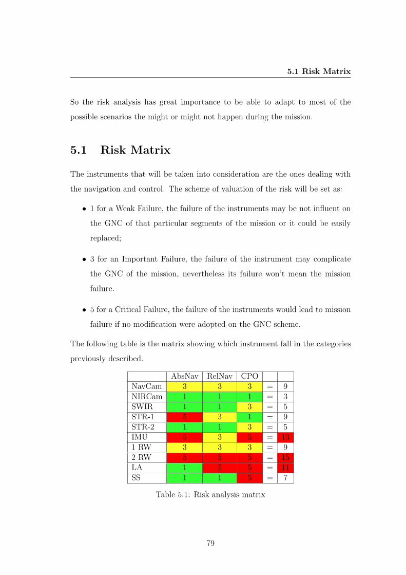
5.1 Risk Matrix
So the risk analysis has great importance to be able to adapt to most of the
possible scenarios the might or might not happen during the mission.
5.1 Risk Matrix
The instruments that will be taken into consideration are the ones dealing with
the navigation and control. The scheme of valuation of the risk will be set as:
• 1 for a Weak Failure, the failure of the instruments may be not influent on
the GNC of that particular segments of the mission or it could be easily
replaced;
• 3 for an Important Failure, the failure of the instrument may complicate
the GNC of the mission, nevertheless its failure won’t mean the mission
failure.
• 5 for a Critical Failure, the failure of the instruments would lead to mission
failure if no modification were adopted on the GNC scheme.
The following table is the matrix showing which instrument fall in the categories
previously described.
AbsNav RelNav CPONavCam 3 3 3 = 9NIRCam 1 1 1 = 3SWIR 1 1 3 = 5STR-1 5 3 1 = 9STR-2 1 1 3 = 5IMU 5 3 5 = 131 RW 3 3 3 = 92 RW 5 5 5 = 15LA 1 5 5 = 11SS 1 1 5 = 7
Table 5.1: Risk analysis matrix
79
5.1 Risk Matrix
In this section, the top 3 critical instruments will be analyzed, namely the case
in which 2 Reaction Wheel fail, the IMU failure and the failure of the Laser
Altimeter (LA).
5.1.1 Reaction Wheel failure
The major problem in the failure of one or two Reaction Wheels is in the attitude
control of the spacecraft. This was the case of the Hayabusa mission, so the first
reference to look up to are the papers published to counter that problem in that
specific case and adapt those solutions to the actual mission.
The main way to control the attitude without the control momentum devices is
through the RCS and the gimballed thruster of the EPS. So an attitude control
algorithm based only on those actuators shall be developed as a backup solution.
5.1.2 IMU failure
The IMU is an instrument indicating the total acceleration and angular rate of
the vehicle in which it is installed by combining the use of an accelerometer and
a gyroscope.
During AbsNav the spacecraft state is estimated through an EKF which take as
input the IMU and Star Tracker measurements. Without the IMU the spacecraft
shall navigate using only the Star Tracker. In this case two possible scenarios
could be considered:
• Continue Deep Space navigation mode until the beginning of RelNav;
• if the accuracy of the ephemerides is high enough, try to navigate by using
the Star Tracker.
In the following phases since no information about the velocity can be obtained,
the spacecraft shall estimate its velocity from the rate of change in the size of the
80
5.1 Risk Matrix
asteroid image and make maneuvers based on that estimation, until it reaches
the distance in which the LA can be used and the velocity can be determined.
The whole process should be monitored from ground for a more refined result.
5.1.3 Laser Altimeter failure
Laser altimeter is a fundamental instrument, especially in the last part of the
mission since it gives exact information about the relative state and it is very
important for building the asteroid 3D model.
To counter this failure the spacecraft needs at least one range measurement pro-
vided by ground to relate that distance to an image of the asteroid and perform
coarse navigation relative to the small body. By knowing the dimension of the
asteroid at a certain distance the spacecraft can estimate its position through a
simple proportion
dnpx = dradionradiopx
npx
(5.1)
The 3D model instead cannot be precisely determined since the model shall be
based only on the NavCam images, for example exploiting the Silhouette and the
Shadow Carving Methods already used in the Rosetta mission.
81
Chapter 6
Conclusions
The thesis addressed the problem of a Cubesat, which by definition has limited
capabilities, to reach a small body, a celestial object small enough to consider
negligible its gravitational field.
A series of operations were defined for the R&CPO, which was divided in sub-
phases depending on the instruments that were used:
• Absolute Navigation Phase, the navigation was performed using informa-
tion from the Star Tracker and IMU.
• the First part of the Relative Navigation Phase, the small body was big
enough to allow relative navigation using information from the Star Tracker,
the NavCam, the NIRCam, and IMU.
• the Second part of the Relative Navigation Phase, the spacecraft in this
phase is close enough to use also the altimeter obtaining exact information
on its relative state.
• Close Proximity Operation Phase, in which the spacecraft is close enough
to map in detail the asteroid surface, determine its geophysical properties
and its dynamic state.
82
During the mission it was analyzed how a CoB-based Navigation would perform.
For the last phase the dynamic model was developed and different trajectories
were proposed and analyzed taking into consideration the propellant budget lim-
itation and image quality limitation. To perform this analysis a simulator was
developed, which could be used for the five asteroid that the M-ARGO mission
was planned to visit or it can be used generally by uploading to the kernel folder
the appropriate kernels. These trajectories were also analyzed by loading the
ephemerides in Blender. It was also verified that the spacecraft parameters that
were modified in the MDR could not satisfy any budget requirement, thus leading
to a mission which cost was over twice its actual cost budget.
Lastly, a Severity and Likelihood Categorization was made, analyzing which were
the most critical components in the mission and how a particular breakdown
would compromise the whole mission.
Future work could focus on some aspects that were not addressed on this thesis:
• develop the GNC in the rendezvous phase, considering the impulses as low-
thrust finite burn maneuvers. To address this topic start by referring on
[31];
• work on the chemical composition estimation algorithm, presented in 4.4.4;
• implement the modified navigation algorithms deriving from the breakdown
of a particular component briefly discussed in Chapter 5.
83
References
[1] J. Kawaguchi, A. Fujiwara, and T. Uesugi, “Hayabusa, Rendezvous and Prox-
imity Operations,” 2005.
[2] J. Kawaguchi, T. Kubota, M. Otsuki, T. Hashimoto, N. Bando, H. Yano,
M. Uo, and K. Shirakawa, “Touchdown Dynamics for Sampling in Hayabusa
Mission,” 2006.
[3] J. Kawaguchi, T. Kubota, J.Saito, T. Hashimoto, M. Uo, K. Shirakawa,
H.Morita, N.Muranaka, H. Ohyama, and M. Maruya, “Navigation Shape
and Surface Topography Model of Itokawa,” 2006.
[4] T. Morley, F. Budnik, B. Godard, P. Munoz, and V. Janarthanan, “Rosetta
Navigation from Reactivation until arrival at comet 67P/Churyumov-
Gerasimenko,” 2015.
[5] F. Castellini, D. Antal-Wokes, R. P. de Santayana, and K. Vantournhout,
“Far Approach optical navigation and comet photometry for the Rosetta mis-
sion,” 2015.
[6] M. Lauer, S. Kielbassa, and R. Pardo, “Optical measurements for attitude
control and shape reconstruction at the Rosetta flyby of asteroid Lutetia,”
2012.
84
REFERENCES
[7] N. Aeronautics and S. Administration, “Hayabusa.” https://nssdc.gsfc.
nasa.gov/nmc/spacecraft/display.action?id=2003-019A.
[8] N. Aeronautics and S. Administration, “OSIRIS-REx, Asteroid Sample
Return Mission.” https://www.nasa.gov/sites/default/files/atoms/
files/osiris-rex_press_kit_0.pdf.
[9] E. Gibney, “Duck-shaped comet could make Rosetta
landing more difficult.” https://www.nature.com/news/
duck-shaped-comet-could-make-rosetta-landing-more-difficult-1.
15579.
[10] T. Kominato and M. Matsuoka, “Hayabusa Optical Hybrid Navigation and
Guidance,” 2005.
[11] S. Nishihara, K. Kitazato, M. Abe, S. Hasegawa, M. Ishiguro, H. Nonaka,
Y. Ohba, T. Ozawa, Y. S. a Y. ndYadoumaru, C. Yoshizumi, and M. Okyudo,
“Ground-based lightcurve observation campaign of (25143) Itokawa between
2001 and 2004,”
[12] “LCDB Data.” http://www.minorplanet.info/PHP/
generateOneAsteroidInfo.php?AstInfo=25143%7CItokawa.
[13] J. Kawaguchi, T. Kubota, M. Otsuki, T. Hashimoto, M. Uo, and K. Shi-
rakawa, “Attitude Control Challenges and Solutions for Hayabusa Space-
craft,” 2006.
[14] U. Herfort and C. M. Casas, “Trajectory Preparation for the Approach of SC
Rosetta to comet 67P/Churyumov-Gerasimenko,” 2015.
[15] P. Munoz, F. Budnik, B. Godard, T. Morley, V. Companys, U. Herfort, and
85
REFERENCES
C. Casas, “Preparations and strategy for navigation during Rosetta Comet
Phase,” 2012.
[16] S. Savarese, M. Andreetto, H. Rushmeier, F. Bernardini, and P. Perona, “3D
Reconstruction by Shadow Carving: Theory and Practical Evaluation,” 2006.
[17] S. Savarese, H. Rushmeier, F. Bernardini, and P. Peronaz, “Implementation
of a Shadow Carving System for Shape Capture,” 2002.
[18] ESA, “CDF Study Report: M-ARGO. Assessment of Standalone Interplan-
etary CubeSat Mission,” 2017.
[19] A. Brorsson, “MSc. Thesis: Compressive Sensing: Single Pixel SWIR Imag-
ing of Natural Scenes,” 2018.
[20] D. J. Starling, I. Storer, and G. A. Howland, “Compressive sensing spec-
troscopy with a single pixel camera,” 2016.
[21] A. S. University, “Conversion of Absolute Magnitude to Diameter
for Minor Planets.” http://www.physics.sfasu.edu/astro/asteroids/
sizemagnitude.html.
[22] NASA, “Sentry: Earth Impact Monitoring.” https://cneos.jpl.nasa.
gov/sentry/.
[23] S. S. T. University, “Catalogue of the Solar System Small Bodies Or-
bital Evolution.” http://smallbodies.ru/en/asteroids/info/general/
2010_UE51/.
[24] B. Carry, “Density of Asteroids,” 2012.
[25] ESA, “Shape model of Comet 67P/C-G.” https://sci.esa.int/web/
rosetta/-/54728-shape-model-of-comet-67p.
86
REFERENCES
[26] NASA, “Asteroid Itokawa 3D Model.” https://solarsystem.nasa.gov/
resources/2377/asteroid-itokawa-3d-model/.
[27] C. Acton, “Ancillary Data Services of NASA’s Navigation and Ancillary
Information Facility,” pp. Planetary and Space Science, Vol. 44, No. 1, pp.
65–70, 1996.
[28] B. S. E. W. Charles Acton, Nathaniel Bachman, “A look to-
ward the future in the handling of space science mission geom-
etry,” Planetary and Space Science, DOI 10.1016/j.pss.2017.02.013,
https://doi.org/10.1016/j.pss.2017.02.013, 2017.
[29] H. D. Curtis, “Orbital Mechanics for Engineering Students,” 2010.
[30] M. Okasha and B. Newman, “Relative Motion Guidance, Navigation and
Control for Autonomous Orbital Rendezvous,” 2012.
[31] D. A. D. Tos, M. Rasotto, F. Renk, and F. Topputo, “LISA Pathfinder
mission extension: A feasibility analysis,” 2019.
[32] P. L. Lamy, I. Toth, H. A. Weaver, L. Jorda, M. Kaasalainen, and P. J. Gutir-
rez, “Hubble Space Telescope observations of the nucleus and inner coma of
comet 67P/Churyumov-Gerasimenko,” 2006.
[33] D. J. Scheeres, “Close proximity operations at small bodies: orbiting, hover-
ing, and hopping,” 2004.
[34] S. Jin, W. Hui, Y. Wang, K. Huang, Q. Shi, C. Ying, D. Liu, Q. Ye, W. Zhou,
and J. Tian, “Hyperspectral imaging using the single-pixel Fourier transform
technique,” 2017.
[35] C. Olson, R. P. Russell, and S. Bhaskaran, “Spin State Estimation of Tum-
bling Small Bodies,” 2016.
87

REFERENCES
[36] A. Petit, J. Souchay, and C. Lhotka, “High precision model of precession and
nutation of the asteroids (1) Ceres, (4) Vesta, (433) Eros, (2867) Steins, and
(25143) Itokawa,” 2014.
88