renormalization and supersymmetry breaking phenomenology
TRANSCRIPT

Thesis for the Degree of Master of Science in Physics
Renormalizationand
SupersymmetryBreaking Phenomenology
Par Pettersson
Fundamental PhysicsChalmers University of Technology
Jan 2011

Renormalization and Supersymmetry Breaking PhenomenologyPar Pettersson
c⃝ Par Pettersson, 2011
Department of Fundamental PhysicsChalmers University of TechnologySE-412 96 Goteborg, SwedenTelephone + 46 (0)31-772 1000
Chalmers ReproserviceGoteborg, Sweden 2011
Renormalizationand
Supersymmetry Breaking PhenomenologyPar Pettersson
Department of Fundamental PhysicsChalmers University of Technology
SE-412 96 Goteborg, Sweden
Abstract
In this thesis we address some issues of current interest in particle physics andquantum field theory (QFT).
First we give an introduction to renormalized perturbation theory andloop computations in QFT. Quantum chromodynamics (QCD) is used as anexample and it is explicitly renormalized to first order, with all countertermscomputed. The β-function is derived and used to show that QCD is asymp-totically free.
Secondly we give a short introduction to supersymmetry (SUSY): thealgebra, superfields and SUSY breaking. We present a simple model (theO’Raifeartaigh model) and show how to deal with the case of strong SUSYbreaking in a manifestly supersymmetry invariant way.
Finally we compute the tree level cross section for production of a hiddenvector boson present in a specific model of SUSY breaking (semi-direct gaugemediation). Unfortunately, the resulting cross section is too small to give asignal at the LHC. We also compute the decay rate of the vector boson andshow that it is actually a candidate for dark matter.
AcknowledgmentsMy greatest gratitude goes to my supervisor Gabriele Ferretti for all his
ideas and guidance through the maze that is particle physics. No subject wasconsidered too remote and no question went unanswered, more often than notthey developed into a discussion deserving its own lecture.
My second greatest thanks goes to my good friend Hampus Linander forhis perpetual company when getting coffee, and his superhuman ability inasking that ’But why...’-question that I could never answer. It always sent mestraight back to my desk, questing for better understanding.
I would also like to thank past and present members at the Institution ofFundamental Physics for all help, interesting discussions, ’fredagsfika’, ’lunch-lopning’ and, most of all, for providing a very pleasant and welcoming atmo-sphere where a confused master student can conduct his (or her) studies.
Finally, I would like to thank my family: Inger, Lasse, Jon and Sivert,without whose support (though generally more concerned with how I wasdoing than the specifics of what I did) I would never have dared take the stepinto what is considered one of the most difficult areas in existence.

”Nothing travels faster than the speed of light with the possibleexception of bad news, which obeys its own special laws.”
– Douglas Adams (chapter one of ’Mostly Harmless’)


Contents
1 Introduction 11.1 Method . . . . . . . . . . . . . . . . . . . . . . . . . . . . . . . 4
2 Asymptotic Freedom in QCD 52.1 The Problem with Divergences . . . . . . . . . . . . . . . . . . 52.2 Renormalizing a Non-Abelian Gauge Theory . . . . . . . . . . 82.3 Computing Loops and Counterterms . . . . . . . . . . . . . . . 112.4 The β-function of QCD . . . . . . . . . . . . . . . . . . . . . . 16
3 Some Introductory Supersymmetry 223.1 Basic SUSY . . . . . . . . . . . . . . . . . . . . . . . . . . . . . 223.2 The Superfield Formalism . . . . . . . . . . . . . . . . . . . . . 27
4 A SUSY Breaking Sector 334.1 A SUSY Breaking Model . . . . . . . . . . . . . . . . . . . . . 334.2 An Effective Field Theory . . . . . . . . . . . . . . . . . . . . . 36
5 An Experimental Sign of SUSY Breaking 425.1 Producing the Hidden Particles . . . . . . . . . . . . . . . . . . 435.2 Decay of the Hidden Particle . . . . . . . . . . . . . . . . . . . 47
A Conventions 50
B Ghosts 52
C QCD Counterterms 55C.1 The Gluon Counterterm . . . . . . . . . . . . . . . . . . . . . . 55C.2 The Vertex Counterterm . . . . . . . . . . . . . . . . . . . . . . 60
D Calculus in Superspace 63
Bibliography 65
vii


1Introduction
During my fourth year of study I took a course in quantum field theory (QFT).I found it extremely complicated and to my great regret (and horror!) I failed,even though I knew that it is the basic groundwork for all particle physics, inwhich I have a great interest. After having thought about how to face my fearof the subject for the better part of a year, I finally realized that the only wayI was ever going to learn, was by putting myself in a position where I had noother choice. That said, I obviously had to do my master thesis on a subjectconnected to quantum fields! In retrospect I have to say that even though thelogic seems flawed, I have not regretted the decision at all.
The goal of a particle physicist is to describe the basic constituents of mat-ter and how it works, because from there virtually all physics can be derived.Ideas about the smallest parts of nature have been around for centuries, but in1789 the French chemist A. Lavoisier (who was later executed in 1794 duringthe French revolution, to which Lagrange responded: ’It took them only aninstant to cut off his head, but France may not produce another such headin a century.’) defined an element as a basic substance that could not bebroken down, and this was termed an atom. Around a hundred years later(1897) it was shown that the atom was not the smallest constituent, when thenegatively charged electron was discovered by J.J Thompson.
In 1909 an experiment led by E. Rutherford discovered the atomic nucleus.Two years later he suggested a model where the atom was built out of anucleus, where most of the mass is concentrated, and a number of electronscircling around it (at a distance of roughly 10−10 m = 1 A). The nucleus wasfurthermore shown to be built out of the positively charged protons (found byRutherford in 1915) and neutrons (found by J. Chadwick in 1932) and thesewere later shown to have roughly the size 10−15 m.
In the 60’s M. Gell-Mann and G. Zweig proposed on theoretical groundsthat all hadrons, including protons and neutrons, are in turn composite par-
1

2 Chapter 1: Introduction
Figure 1.1: The molecule in the top left is built from hydrogen, carbon andoxygen atoms, and each of these consist of a nucleus with electrons around it.The nucleus is built out of protons and neutrons, which are in turn composedof three quarks each. It is unknown whether quarks and electrons have anyinner structure and as far as we know they behave as points (they could, forexample, be strings). The size of the molecule (Thujone, C10H16O) is typically10−9 m, the atom 10−10 m and the nucleus 10−15 m.
ticles consisting of quarks1. This proposal was verified in 1968 and today it isstill the accepted model. At the time of writing six different types of quarkshave been found. An illustration of the situation is shown in figure 1.12.
Furthermore, the electron have two heavier cousins: the muon and the tau.Along with the neutrinos, which interact very weakly with matter, they are
1The baryons, to which protons and neutrons belong, consist of three quarks whereas themesons are built out of two: a quark and an anti-quark.
2The picture is composed from the following images: the molecule:http://czechabsinthe.files.wordpress.com/2007/04/molecule.jpg; the atom:http://stuffthathappens.com/blog/wp-content/uploads/2007/11/atom.png; thenucleus http://www.theo-phys.uni-essen.de/tp/ags/guhr_dir/media/nucleus3.jpg;the proton http://upload.wikimedia.org/wikipedia/commons/9/92/Quark_structure_proton.svg.
3
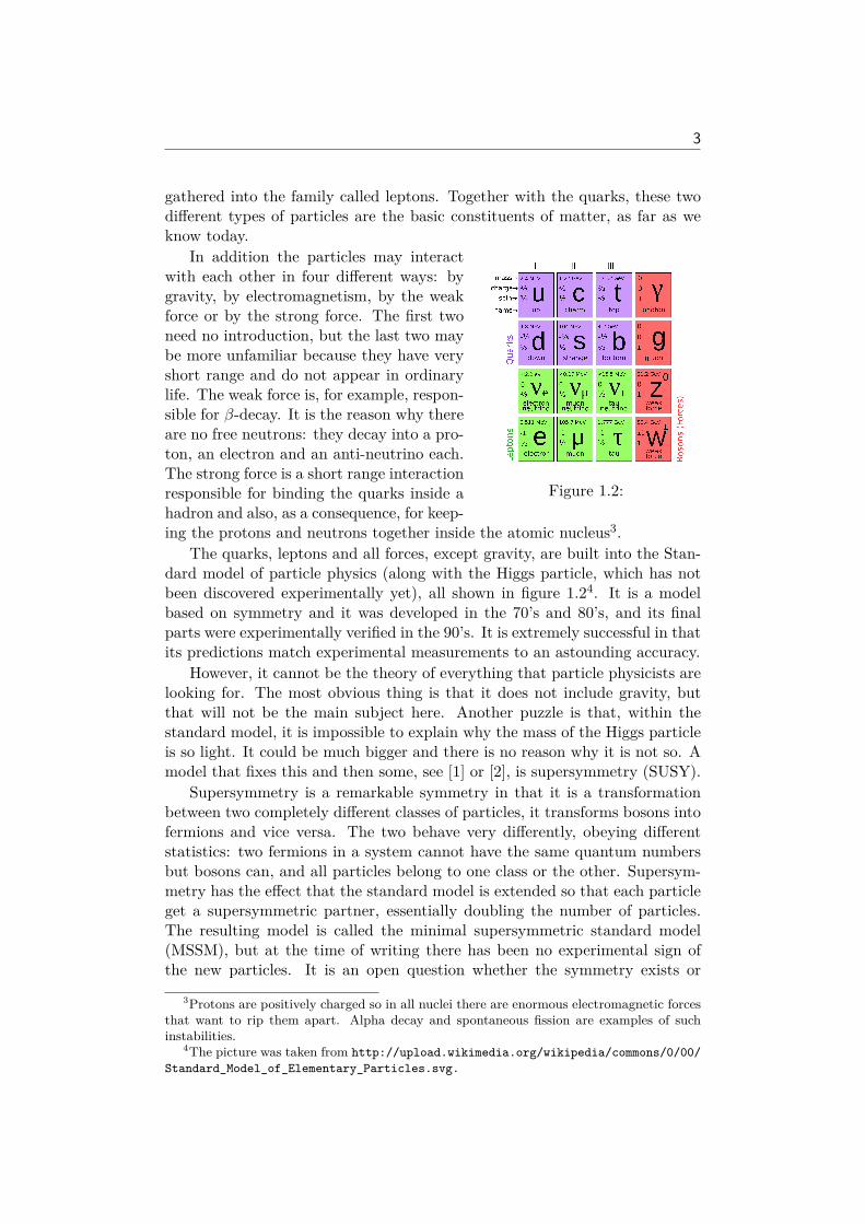
gathered into the family called leptons. Together with the quarks, these twodifferent types of particles are the basic constituents of matter, as far as weknow today.
Figure 1.2:
In addition the particles may interactwith each other in four different ways: bygravity, by electromagnetism, by the weakforce or by the strong force. The first twoneed no introduction, but the last two maybe more unfamiliar because they have veryshort range and do not appear in ordinarylife. The weak force is, for example, respon-sible for β-decay. It is the reason why thereare no free neutrons: they decay into a pro-ton, an electron and an anti-neutrino each.The strong force is a short range interactionresponsible for binding the quarks inside ahadron and also, as a consequence, for keep-ing the protons and neutrons together inside the atomic nucleus3.
The quarks, leptons and all forces, except gravity, are built into the Stan-dard model of particle physics (along with the Higgs particle, which has notbeen discovered experimentally yet), all shown in figure 1.24. It is a modelbased on symmetry and it was developed in the 70’s and 80’s, and its finalparts were experimentally verified in the 90’s. It is extremely successful in thatits predictions match experimental measurements to an astounding accuracy.
However, it cannot be the theory of everything that particle physicists arelooking for. The most obvious thing is that it does not include gravity, butthat will not be the main subject here. Another puzzle is that, within thestandard model, it is impossible to explain why the mass of the Higgs particleis so light. It could be much bigger and there is no reason why it is not so. Amodel that fixes this and then some, see [1] or [2], is supersymmetry (SUSY).
Supersymmetry is a remarkable symmetry in that it is a transformationbetween two completely different classes of particles, it transforms bosons intofermions and vice versa. The two behave very differently, obeying differentstatistics: two fermions in a system cannot have the same quantum numbersbut bosons can, and all particles belong to one class or the other. Supersym-metry has the effect that the standard model is extended so that each particleget a supersymmetric partner, essentially doubling the number of particles.The resulting model is called the minimal supersymmetric standard model(MSSM), but at the time of writing there has been no experimental sign ofthe new particles. It is an open question whether the symmetry exists or
3Protons are positively charged so in all nuclei there are enormous electromagnetic forcesthat want to rip them apart. Alpha decay and spontaneous fission are examples of suchinstabilities.
4The picture was taken from http://upload.wikimedia.org/wikipedia/commons/0/00/Standard_Model_of_Elementary_Particles.svg.

4 Chapter 1: Introduction
not, but it is widely considered to be the most promising model for physicsbeyond the standard model. Fortunately, with the start of the Large HadronCollider (LHC) in 2010, we are on the brink of discovering whether it reallydoes describe reality or not.
The main subject here will be supersymmetry: how to break it and thephenomenology of the breaking. When writing a thesis there is usually onespecific question that must be answered, but it is difficult to state one singlequestion for this problem. Instead the purpose has been to acquire enoughknowledge and skill to be able to understand the latest research material onthe subject.
As for the report itself, there is some thought behind what has been in-cluded and what has been left out. The first section deals with renormalizationand loop computations in QFT, necessary for essentially any advanced phe-nomenological application. The next chapter develops the basic working toolsof supersymmetry in superspace. The methods of both sections are then usedwhen working with the theory presented in section 4. In the final section weapply (a more complicated version of) the theory of the previous chapter toexamine the phenomenology.
1.1 MethodThe method is a combination of a literature study (the most important booksand papers used in each section are listed in their respective introduction), aseries of discussions and some theoretical research. In sections 2 and 3 thetools were books, papers and discussions with my supervisor. In sections 2.3and 2.4 we review a specific example, originally worked out in the 70’s by D.Gross, H. Politzer and F. Wilczek.
The final two chapters contain some new theoretical results that have notbeen previously published. The work has been carried out in collaborationwith my supervisor, whom deserves the credit for all ideas. The computationshave been done by both of us separately and then compared.

2Asymptotic Freedom in QCD
Tree level quantum field theory computations often give good predictions,however if one wants to compute higher order corrections, to get even betterresults, trouble arises. Often the corrections seem to be infinite, a predictionthat does not go well with reality because experimentalists measure finite re-sults. The solution to this problem offers a great deal of new physical insight.In principle, to be able to go on into more advanced matters in quantum fieldtheory, such as supersymmetry, one has to learn about loops and renormaliza-tion.
The outline for the section is the following: the first part will introducethe problem and offer some qualitative explanation to why it appears. Thefollowing two sections treat it and show how computations can be performed,using quantum chromodynamics (QCD, the theory of quarks and gluons) as anexample. This is far from the easiest theory to work with but it is satisfying,because as the computations become more and more complicated so does thephysics. In the last part of the section, the concepts introduced so far areused and treated in a way that offers a more natural interpretation. The goalis to show that QCD is asymptotically free, i.e can be treated perturbativelyat high energies. This is a computation that was done already in 1973 byH. Politzer, D. Gross and F. Wilczek and won them the Noble prize in 2004.Good introductions to the subject are [3] and [4].
2.1 The Problem with DivergencesThe first impression you get from renormalization is usually how ugly it is.You hear that the theory actually predicts infinities when you compute crosssections and that you, somehow, are able to shove them away into some cornerand then leave them there to rot. The experimentalist do not measure infinitecross sections and so, you think, the theoreticians just try to lie the infinitiesaway to make the theory fit reality.
5

6 Chapter 2: Asymptotic Freedom in QCD
This is as far from the truth as you can get. When you start working withit and understand more and more you soon realize, at least that is what I did,how subtle and beautiful it really is. But it is not all about understanding,it takes some getting used to also. Even though you are comfortable withit, there will be times when you are in the middle of a computation and yousuddenly start thinking ’what am I really doing?’.
To see where the problem arises we will use ϕ4-theory as a basic example.It is defined by the familiar Lagrangian
L = 12∂µϕ∂
µϕ− 12m2ϕ2 − λ
4!ϕ4 (2.1)
Even with this basic example it is impossible to compute the propagatorsexactly. This is nothing strange to physicists and the way to handle it is thesame as in non-relativistic quantum mechanics - we use perturbation theory.Let us compute the four-point interaction: there are two incoming particleswith four-momenta pµ1 and pµ2 that scatter into the two outgoing particles withqµ1 and qµ2 . The probability of scattering is gotten by time evolving both statesand computing the overlap
limT→∞
⟨p1, p2| e−2iHT | q1, q2⟩ = iMδ4(p1 + p2 − q1 − q2) (2.2)
With H the Hamiltonian. The first order perturbation is the tree levelprocess
Mtree = = −iλ
The scattering amplitude is |M|2tree= λ2 and it is very much finite. If wewant to get a more precise result we have to go on and compute the secondorder perturbation. This will be of order λ2 and if λ < 1, which it must be ifperturbation theory is to work, the second order contribution should probablybe a lesser correction.
M2 = + +
We only have to compute the first diagram, the s-channel process1.1Technically speaking it is not really a s-channel because the outgoing propagators cannot
form a bound state and thus there is no pole. I call it s-channel because the diagrammaticform is similar to such processes.

2.1 The Problem with Divergences 7
M2 = −λ2∫
d4k
(2π)41
k2 −m2 + iε
1(k + p1 + p2)2 −m2 + iε
(2.3)
But this is suspicious: there are four powers of momenta both in the nu-merator and the denominator so the integral could diverge. We are interestedin large momenta so assume k2 >> p2
1, p22. Let k0 → ik0 to get an Euclidean
metric
M2 ∼ −λ2∫
d4k
(2π)41
(k2 +m2)2 = −λ2 Ω3(2π)4
∫dk
k3
(k2 +m2)2
∼ limk→∞
−λ2
2Ω3
(2π)4 log k2 +m2
m2 (2.4)
This is the famous logarithmic divergence of quantum field theory! Doesthis mean that the whole theory is complete nonsense? To answer that we willneed to discuss experimental measurements and QED may be more suitablefor that purpose, as it is easier to use physical intuition. Therefore considerthe scattering of two electrons into to muons. The full scattering process isgiven by
e− µ−
e+ µ+
= + +
+ + + + (all orders)
The logarithmic divergences appear here as well, the three last diagramson the right-hand side have such behaviour while the top two loop diagramsare finite. Despite the fact that the theory suggests divergences, experimentsmeasure the left-hand side and they get finite results. An estimate of the crosssection using only the tree level result gives the correct order of magnitude forthe scattering (see [5]). In other words the theory behave as we would expectif we didn’t know about the divergences. Let us ponder what physically mayhappen inside the loop
When computing the scattering amplitude the particle circling inside theloop was allowed to have any momentum, in other words, arbitrarily highenergy. In the most extreme case the particle would have energy of the orderof the Planck mass and we would have to start worrying about black holes.Quantum field theory cannot handle that because it knows nothing aboutquantum gravity. At that energy, and probably long before that2, the theory
2For the specific case of QED, it breaks down already around 100 GeV when electroweakeffects become important.

8 Chapter 2: Asymptotic Freedom in QCD
breaks down. Conversely the appearance of infinities tells us that quantumfield theory is a good model, because when there are effects it cannot handleit is intelligent enough to give a warning sign. It would be a lot worse ifeverything came out finite but did not agree with experiments. The trueunderlying theory should be free of infinities (note that string theory is) butat least there is a reason why they pop up in these computations.
The divergences discussed here are called ultraviolet divergences. There isanother type of divergence, called infrared, that comes about because for anyprocess containing a massless propagator, there will be a pole as its momentumapproaches zero. Although it is an interesting subject it can be solved inde-pendently of renormalization. It will not be treated here but a good treatmentcan be found in [6] and [7].
A final comment: note that what was done so far was computing loops, thisis not renormalization! Renormalization is the process where the divergencesare built into the theory by reinterpreting the fields, masses and couplingconstants as actually containing them from the start and making a distinctionbetween the measurable physical quantities and theoretical bare quantities.QCD will be used next as an example to really step up the difficulty.
2.2 Renormalizing a Non-Abelian Gauge Theory
In the previous section the appearance of the divergences was explained. Herethe plan of attack is to interpret them and make them a natural part of thetheory, this is what is called renormalization. There are several ways to doit and the one used here is called renormalized perturbation theory. It issuitable for computing physical quantities such as cross sections, but there aremore sophisticated methods that offer greater physical insight. In the end, allmethods must of course give the same result for an observable quantity.
In section 2.3 we will compute loops and to do so the integrals must beregulated to preserve gauge invariance. For this matter we will have to workin d-dimensions (d − 1 space dimension), only taking the limit d → 4 in thevery end. Therefore everything in this section is also done for a d-dimensionalspacetime.
As example a SU(3) gauge theory will be used. The Lagrangian, calledthe Yang-Mills Lagrangian, is
L = −14F a0µνF
µνa0 + ψ0(i/∂ −m0)ψ0 + g0ψ0γ
µT aψ0Aa0µ (2.5)
With F a0µν the field strength of the gluon field
F a0µν = ∂µAa0ν − ∂νA
a0µ + g0f
abcAb0µAc0ν (2.6)
The index 0 on the fields will be useful to keep this Lagrangian separatefrom the renormalized one. Equation (2.5) does not look very much differentfrom the Lagrangian of QED except for the generators T a (which are actually

2.2 Renormalizing a Non-Abelian Gauge Theory 9
1/2 times the Gell-Mann matrices) but some care is needed. In addition to theusual hidden spinor indices ψ has an additional hidden index, since it belongsto the fundamental representation of SU(3) (ψ is in the anti-fundamental).This is contracted with the hidden indices on T a in the same way the spinorindices are contracted with γµ. When all non-linear terms are written outthere are a lot of new interactions
L0 = ψ0(i/∂−m0)ψ0−14
(∂µA
a0ν − ∂νA
a0µ
)(∂µAνa0 − ∂νAµa0 )+g0ψ0γ
µT aψ0Aa0µ
− g0fabc(∂µAa0λ)Aµb0 A
λc0 − 1
4g2
0(feabAa0µAb0ν)(fecdAµc0 A
νd0 ) (2.7)
From now on this will be refereed to as the bare Lagrangian and the fieldswith index 0 will be the bare fields. Actually, additional terms will have tobe added later on to account for gauge invariance, but they will not affect thediscussion here. This is further commented in appendix B.
The first step in the renormalization process is a rescaling of the bare fields
Aa0µ =√ZAA
aµ, ψ0 =
√Zψψ (2.8)
This is the first place the infamous divergences appear in loop calculations.What we have changed is the normalization of the fields and it is divergent asd → 4 but as long as d is arbitrarily small there is no cause for alarm. Puttingthis back into the Lagrangian yields
L = Zψψ(i/∂ −m0)ψ − 14ZA
(∂µA
aν − ∂νA
aµ
)(∂µAνa − ∂νAµa)
+ g0Zψ√ZAψγ
µT aψAaµ − g0Z3/2A fabc(∂µAaλ)AµbAλc
− 14g2
0Z2A(feabAaµAbν)(fecdAµcAνd) (2.9)
Unfortunately the coupling constant acquired a unit when going to d-dimensions. In practice this is not a problem but it would be nice to keepit dimensionless. The dimensions of the fields in an arbitrary dimension canbe worked out by looking at the kinetic terms and any of the interactions.They are, in units of energy,
[L] = Ed, [ψ] = E(d−1)/2, Aµ = Ed/2−1, [g0] = E(4−d)/2
To get a dimensionless coupling constant, substitute√ZAZψg0 = Zgµ
εg,where [g] = E0, [µ] = E1 and 2ε = 4 − d. The downside here is that in anycomputation where previously only g0 appeared we will have to drag aroundan extra factor of µε. The same thing can be done to the other interactions.
Z3/2A g0 = Z3µ
εg ⇒ Z3 = ZAZgZψ
Z2Ag0 = Z4µ
εg ⇒ Z4 = Z3/2A
ZgZψ
(2.10)

10 Chapter 2: Asymptotic Freedom in QCD
The indices 3 and 4 may seem arbitrary, but they have been chosen be-cause the interactions describe three- and four-point vertices. These are notindependent, because it is the coupling constant that is redefined (not thevertices themselves) and gauge invariance guarantees that it is the same forall interactions.
The Lagrangian in equation (2.9) does not look canonically normalized. Toget it in a form we are used to, that is, in a form where it is more apparent whatthe Feynman rules are, the wavefunction renormalizations must be removedin some way. Rescaling again would achieve nothing except getting back tothe bare version. Instead we will do something that at first may seem foolish:we rewrite the Zs as Z = 1 + δ, effectively breaking up the Lagrangian in acanonically normalized part and additional interaction terms. The new termsare called counterterms and are defined by
δA = ZA − 1, δψ = Zψ − 1, δm = Zψm0 −mδg = Zg − 1, δ3 = Z3 − 1, δ4 = Z4 − 4 (2.11)
With them we rewrite the Lagrangian to its final form
L = ψ(i/∂ −m)ψ − 14
(∂µA
aν − ∂νA
aµ
)2+ µεgψγµT aψAaµ
− µεgfabc(∂µAaλ)AµbAλc − 14µ2εg2(feabAaµAbν)(fecdAµcAνd) + LCT
(2.12)
LCT = ψ(iδψ /∂ − δm)ψ − 14δA(∂µA
aν − ∂νA
aµ
)2+ µεgδgψγ
µT aψAaµ
− µεgδ3fabc(∂µAaλ)AµbAλc − 1
4µ2εg2δ4(feabAaµAbν)(fecdAµcAνd)
(2.13)
This is the renormalized Lagrangian. The price we pay to reinterpretthe divergences is that the theory has to be defined at some energy scale,otherwise the counterterms cannot be specified. This scale is arbitrary andthe renormalization parameter will affect the theoretical results. In practiceit means that the general behaviour of a process can be predicted, but nonumbers can be given unless we first go to an experimentalist and ask howbig a (for example) cross section is at a specific energy. For example: nocalculation in QED will ever tell us how big the fine-structure constant is,but once it is known from experimental measurements, there is no end to thepotential applications of QED.
Setting this scale is next on the agenda. By fixing the propagators andvertices at the scale µ, the counterterms and thus the entire theory can bespecified. Remember that QCD is non-perturbative at low energies so it wouldnot be clever to choose the renormalization scale as the mass of one of the lightquarks. Instead µ must be chosen to at least a few GeV. The theory is definedby the diagrams in figure 2.1, with the conditions

2.3 Computing Loops and Counterterms 11
p= i
/p+m
p2 −m2 + iε− iΣ(/p)
pµ ν = −i ηµνδ
ab
p2 + iε+ iΠabµν(p2)
qµ
pλ1 pκ2
= igΓµ(p1, p2)Da
Figure 2.1: The QCD renormalization diagrams
dd/p
Σ(/p) = 0, p2 = µ2
Σ(/p) = 0, p2 = µ2
Πabµν(p2) = 0, p2 = µ2
Γµ = igγµT a, p21 = p2
2 = µ2
(2.14)
At this point we can solemnly state that QCD has been renormalized!The divergences have been reinterpreted into the definitions of the fields andthe coupling constant. The three- and four-point gluon interactions could bespecified as well, but those counterterms will be given in terms of the othersby equations (2.10) and (2.11). In practice this is not the end of the road.The loop diagrams still need to be computed to get the counterterms, if thetheory is to be used beyond tree level.
2.3 Computing Loops and Counterterms
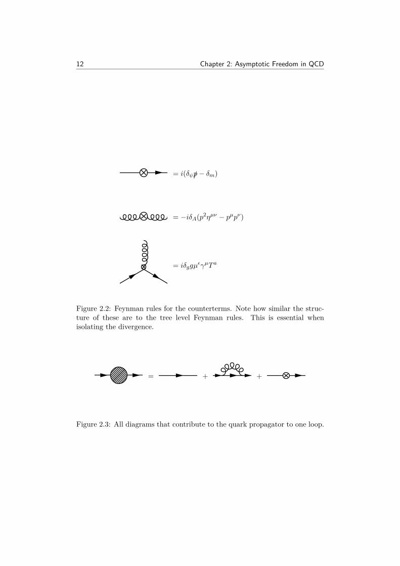
The aim of this section is to compute the divergent parts of the countertermsto one loop. The first thing we need is the Feynman rules for the relevantterms in LCT (see e.g [3]), shown in figure 2.2.
For a theory that is as complicated as QCD computing loops is ratherhard. The only diagram that will be treated here is the first order loop cor-rection to the quark propagator. The rest of the diagrams that come into thecomputation of the counterterms are found in appendix C.
To first order, the diagrams contributing to the quark propagator are shownin figure 2.3. Write the rhs according to figure 2.1
12 Chapter 2: Asymptotic Freedom in QCD
= i(δψ/p− δm)
= −iδA(p2ηµν − pµpν)
= iδggµϵγµT a
Figure 2.2: Feynman rules for the counterterms. Note how similar the struc-ture of these are to the tree level Feynman rules. This is essential whenisolating the divergence.
= + +
Figure 2.3: All diagrams that contribute to the quark propagator to one loop.
2.3 Computing Loops and Counterterms 13
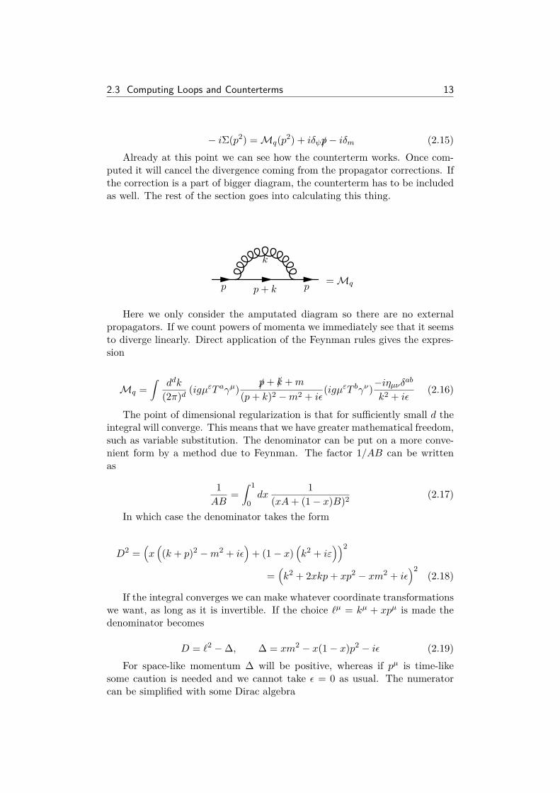
− iΣ(p2) = Mq(p2) + iδψ/p− iδm (2.15)Already at this point we can see how the counterterm works. Once com-
puted it will cancel the divergence coming from the propagator corrections. Ifthe correction is a part of bigger diagram, the counterterm has to be includedas well. The rest of the section goes into calculating this thing.
p p+ k
k
p= Mq
Here we only consider the amputated diagram so there are no externalpropagators. If we count powers of momenta we immediately see that it seemsto diverge linearly. Direct application of the Feynman rules gives the expres-sion
Mq =∫
ddk
(2π)d(igµεT aγµ) /p+ /k +m
(p+ k)2 −m2 + iϵ(igµεT bγν)−iηµνδab
k2 + iϵ(2.16)
The point of dimensional regularization is that for sufficiently small d theintegral will converge. This means that we have greater mathematical freedom,such as variable substitution. The denominator can be put on a more conve-nient form by a method due to Feynman. The factor 1/AB can be writtenas
1AB
=∫ 1
0dx
1(xA+ (1 − x)B)2 (2.17)
In which case the denominator takes the form
D2 =(x((k + p)2 −m2 + iϵ
)+ (1 − x)
(k2 + iε
))2
=(k2 + 2xkp+ xp2 − xm2 + iϵ
)2(2.18)
If the integral converges we can make whatever coordinate transformationswe want, as long as it is invertible. If the choice ℓµ = kµ + xpµ is made thedenominator becomes
D = ℓ2 − ∆, ∆ = xm2 − x(1 − x)p2 − iϵ (2.19)For space-like momentum ∆ will be positive, whereas if pµ is time-like
some caution is needed and we cannot take ϵ = 0 as usual. The numeratorcan be simplified with some Dirac algebra

14 Chapter 2: Asymptotic Freedom in QCD
N = γµ(/ℓ + (1 − x)/p+m
)γµ = (2 − d)(/ℓ + (1 − x)/p) + dm (2.20)
Next consider the Lie algebra factor. The gauge group is SU(3) but it ismore convenient to keep it completely general, to keep the integration con-stants separate from the Lie algebra constants. The factor T aT a is the Casimiroperator and commutes with all generators of a simple Lie algebra
[T b, T aT a] = f bacT cT a + f bacT aT c = 0 (2.21)
By Shur’s lemma, it should be proportional to the identity matrix timessome constant C2(r), that may be different for each representation. The finalexpression is
Mq = −g2µ2εC2(r)∫ 1
0dx
∫ddℓ
(2π)d(2 − d)(/ℓ + (1 − x)/p) + dm
(ℓ2 − ∆)2 (2.22)
To evaluate it we make a Wick rotation to get an Euclidean integrationmeasure, by doing the following substitution
ℓ0 = iℓ0w, ℓ = ℓw ⇒ det(dℓ/dℓw) = i (2.23)
With an Euclidean metric it is obvious that any expression with an oddpower of ℓ in the numerator disappears, due to spherical symmetry, becausethe denominator is even and positive for all ℓ. What is left to evaluate is
− ig2µ2εC2(r)∫ 1
0dx
[((2 − d)(1 − x)/p+ dm)
∫ddℓw(2π)d
1(ℓ2w + ∆)2
](2.24)
The easiest way to compute it is to use hyperspherical coordinates. Theintegrand is independent of all angles and they integrate to give the surfacearea of the d − 1 dimensional sphere. The rest could be looked up in a tableor in Mathematica but my secret passion for integrals demands that I do itproperly. To be more general consider the denominator to the n-th power.
∫ddℓw(2π)d
1(ℓ2w + ∆)n
= Ωd−1(2π)d
∫dℓw
ℓd−1w
(ℓ2w + ∆)n
= Ωd−12(2π)d
∫d(ℓ2w) (ℓ2w)d/2−1
(ℓ2w + ∆)n(2.25)
A nice way to evaluate it is to make the substitution x = ∆ℓ2+∆ and then
compare it to the Beta function.
2.3 Computing Loops and Counterterms 15
∫d(ℓ2w) (ℓ2w)d/2−1
(ℓ2w + ∆)n→ ∆d/2−n
∫ 1
0dx (1 − x)d/2−1xn−d/2−1
= ∆d/2−nΓ(n− d/2)Γ(d/2)Γ(n)
(2.26)
Now set n = 2 to get back to the original problem. Using Ωd−1 = 2πd/2
Γ(d/2)and putting everything together, equation (2.24) takes the form
Mq = −ig2µ2εC2(r)Γ(2 − d/2)(4π)d/2
∫ 1
0dx
(2 − d)(1 − x)/p+ dm
∆2− d2
(2.27)
The divergence manifests itself in the Gamma function as it is singularwhen d → 4. Write 2 − d/2 = ε to make it explicit. The Gamma function hasthe nice property that ζΓ(ζ) = Γ(ζ + 1), i.e we can write Γ(ε) = Γ(ε+1)
ε andthe numerator is finite when ε goes to zero. To identify the different partswrite (µ2/∆)ε = exp (ε log(µ2/∆)) and expand in ε. The final expression is
Mq = −ig2C2(r)16π2
∫ 1
0dx((4 − ε)m− (2 − ε)(1 − x)/p
)× 1ε
(1 + ε log
(µ2
∆
)+ O(ε2)
)(2.28)
Note that the 1ε stands for a logarithmic divergence. To fulfill the specified
condition in equation (2.14) the quark and mass counterterms have to takethe value iδψ = − d
d/p(Mq) and i(/pδψ − δm) = −Mq, both conditions evaluated
at p2 = µ2.As can be seen from the above, the finite part of any counterterm can be
changed by a different choice of renormalization scale. This means that theconstant is arbitrary and we do not have to be very specific about it in thecounterterm. Therefore we can define them as
δψ = −g2C2(r)16π2
∫ 1
0dx
2(1 − x)ε
1 + ε log
µ2
∆
∣∣∣∣∣p2=µ2
+ O(ε2)
(2.29)
δm = −g2C2(r)16π2
∫ 1
0dx
4mε
1 + ε log
µ2
∆
∣∣∣∣∣p2=µ2
+ O(ε2)
(2.30)
This is called the minimal subtraction renormalization scheme. For ourpurpose the mass counterterm can be forgotten from now on, because it isunimportant for the β-function. The wavefunction renormalization is vital,however, and the divergent part of it is

16 Chapter 2: Asymptotic Freedom in QCD
limε→0
εδψ = −g2C2(r)16π2 (2.31)
Some comments are needed before the section is concluded. Using dimen-sional regularization here was, strictly speaking, not completely necessary. Theintegrals could have been regulated just as well with the Pauli-Villars method,meaning that another heavy propagating fermion is included in the Lagrangianthat cancels the divergence for very high momenta but does not effect the lowenergy result. Dimensional regularization was used anyway because it is bothmore versatile and not that much more complicated, and therefore there is noreal point in doing anything else. For the gluon counterterm the Pauli-Villarsregulation does NOT work properly.
The rest of the counterterm computations have been placed in appendixC because they are much the same as the one already done, albeit with somecomplications. These are technical issues however and lead to fun calculationsbut it is not much fun to read.
2.4 The β-function of QCDIt has been pointed out several times that the renormalization scale is arbi-trary. It may be worrisome at first that the theory seems not to give uniqueanswers, but the physics must of course be independent of the choice of µ.Therefore no measurable quantity can depend on the renormalization scaleand we may use that to our advantage to derive consistency equations. Thederivation of the β-function is due to ’t Hooft in [8].
Consider the n-point function both in terms of renormalized and bare quan-tities
G(n)(g,m, µ;xνi ) = ⟨Ω|ψ(xν1) . . . ψ(xνn)| Ω⟩
= Z−n/2ψ ⟨Ω|ψ0(xν1) . . . ψ0(xνn)| Ω⟩ = Z
−n/2ψ G
(n)0 (g0,m0, ε;xνi ) (2.32)
The lhs is the renormalized n-point function which is finite and indepen-dent of ε, whereas the correlation function on the rhs is its bare counterpartand independent of the renormalization scale but divergent. If the equationis to be consistent the wavefunction renormalization must be a function of g0,µ and ε such that the dependence on variables are the same on both sidesof the equality, i.e Zψ = Zψ(g0µ
−ε, ε). The combination g0µ−ε must appear
together because Zψ is dimensionless and can therefore only depend on di-mensionless parameters. The spacetime dependence is of no importance hereand the label will be removed from the equations. Note that the wavefunctionrenormalization can always be chosen independent of the (bare) mass3.
3This is not obvious, but it is shown in e.g [9]. The statement is true as long as the energyis greater than the mass of all particles in the theory.

2.4 The β-function of QCD 17
Hold the bare parameters g0 and m0 fixed. The renormalized counterpartsmust then be functions of µ, at least implicitly, to account for the differencebetween renormalized and bare parameters. This reasoning makes clear thedependence on µ and allows us to differentiate both sides of equation (2.32)with respect to it.
d
dµG(n)(g,m, µ) =
[∂g
∂µ
∂
∂g+ ∂m
∂µ
∂
∂m+ ∂
∂µ
]G(n) (2.33)
d
dµ
[Zψ(g0µ
ε, ε)−n/2G(n)0 (g0,m0, ε)
]= −n
2Z
−n/2−1ψ G
(n)0
d
dµZψ
= −n
2G(n) d
dµlogZψ (2.34)
Traditionally this is written as
[µ∂
∂µ+ β(g) ∂
∂g+mγm(g) ∂
∂m+ nγ(g)
]G(n)(g,m, µ) = 0 (2.35)
Where
β(g) = limε→0
µ∂
∂µg(g0µ
−ε, ε) (2.36)
γm(g) = limε→0
−µ ∂
∂µlogZm(g0µ
−ε, ε) (2.37)
γ(g) = limε→0
12µ∂
∂µlogZψ(g0µ
−ε, ε) (2.38)
Finally the β-function has been properly defined. Even though the meth-ods have been purely mathematical its physical meaning is clear: it showshow the coupling constant shifts with the renormalization scale. Since it is adimensionless parameter it must be independent of µ, simply because there isnothing that can kill off its unit.
In the γm equation the Zm is defined as m0 = Zmm, likewise we define g0 =ZGgµ
ε. In the notation of section 2.2 we have ZG = ZG(g, ε) = Zg/√ZAZψ.
Using this for the rhs of the β-function, we have
β(g) = limε→0
µ∂
∂µ
(g0
µεZG
)= lim
ε→0−εg − µgZ−1
G
∂ZG∂µ
(2.39)
But ZG is always computed perturbatively as a function of ε and g
µ∂ZG∂µ
= µ∂g
∂µ
∂ZG∂g
= β(g) ∂∂gZG
Inserting into equation (2.39) results in the Callan-Symanzik equation[εg + gβ(g) ∂
∂g+ β(g)
]ZG(g) = 0 (2.40)

18 Chapter 2: Asymptotic Freedom in QCD
This is a nice result but we can do even better when considering how ZGand β depend on ε, which has to go to zero in the end. If the limit in equation(2.39) exists we can evaluate β as a Taylor expansion in ε, likewise ZG can beexpressed as a Laurent series
β(g) = β(0)(g) + εβ(1)(g) + ε2β(2)(g) + . . .
ZG(g) = 1 + Z(1)G
ε+ Z
(2)G
ε2 + . . .
For the equality in equation (2.40) to hold, the coefficient of every εk mustbe zero. For εn≥2 we get the condition
β(n) + β(n+1)(Z
(1)G + g
∂
∂gZ
(1)G
)+ β(n)
(Z
(2)G + g
∂
∂gZ
(2)G
)+ · · · = 0 (2.41)
The solution is easy to see if the equations are written on matrix form1 (1 + g∂g)Z(1) (1 + g∂g)Z(2) . . .
0 1 (1 + g∂g)Z(1) . . .0 0 1 . . ....
...... . . .
β(2)
β(3)
β(4)
...
= 0 (2.42)
The matrix is triangular so the only solution is the trivial one with everyβ(n) = 0. Using this to write the rest of the equations yields
ε1 : β(1) + g = 0
ε0 : β(0) + β(1)Z(1)G + gZ
(1)G + gβ(1)∂gZ
(1)G = 0
ε−k : β(0)Z(k)G +
(β(1) + gZ
(k)G
)+ gβ(0)∂gZ
(k)G + gβ(1)Z
(k)G = 0
With the solution
β(1) = −g
β = g2∂gZ(1)G (2.43)
β(Z
(k)G + g∂gZ
(k)G
)= g2∂gZ
(k+1)G k ≥ 1
Where we have dropped the index (0). The last equation is for consistency,it is the middle one that is interesting. It says that the β-function ONLYdepends on the simple pole ZG. This is a huge simplification as we do nothave to worry about the finite contributions or higher poles when computingcounterterms (unless we want to do cross sections). Furthermore if we are onlyinterested in the high momentum limit we may work with a massless theory,
2.4 The β-function of QCD 19
because the momentum can be taken sufficiently high to make the mass a veryminor correction. The same methods may be used to derive equations for γmand γ but they will not be used.
The next step is to solve the Callan-Symanzik equation once and for all. Todo so we will work with the two-point correlation function. Due to dimensionalarguments it must be possible to write it as
G(2) = i
p2 f(p2/µ2) (2.44)
For some function f . By using the chain rule we can swap the µ-derivativefor a p
µ∂
∂µG(2) = −
(p∂
∂p+ 2
)G(2) (2.45)
And the Callan-Symanzik equation takes the form[p∂
∂p− β(g) ∂
∂g+ 2 − 2γ(g)
]G(2)(g, p, µ) = 0 (2.46)
The advantage compared to the previous form of the C-S equation is thatnow there is no implicit dependence left. A very nice way to solve it wasworked out by Sidney Coleman (see [10]) who compared it to a fluid, full ofbacteria, running through a pipe. Interpret p as time, β as velocity, γ asgrowth rate and G(2) as a density. Do the following substitutions
log (p/µ) = tg = x
−β(g) = v(x)2γ(g) − 2 = ρ(x)G(2)(p, g) = D(t, x)
The C-S equation becomes[∂
∂t+ v(x) ∂
∂x− ρ(x)
]D(t, x) = 0 (2.47)
The bacterial density is the unknown function D(t, x), with ρ(x) being therate of growth, x the position in the pipe and v(x) the speed of the water. Ifwe take the Lagrangian viewpoint and travel with the water the equation issimple, as the velocity term disappears. The solution in this case is the sameas for a stationary situation, i.e some initial density Di(x) integrated with thegrowth rate along the path x(t). The problem reduces to finding the trajectoryof a fluid element in the running water to get back to the Euclidean picture.
d
dtx(t, x) = −v(x), x(0, x) = x (2.48)
Combining the two will give the full solution

20 Chapter 2: Asymptotic Freedom in QCD
D(t, x) = Di(x(t, x)) exp(∫ t
0dt′ ρ(x(t′, x))
)= Di(x(t, x)) exp
(∫ x
x(t)dx′ ρ(x′)
v(x′)
)(2.49)
Curiously, the trajectory equations are at least as interesting as the fullsolution. In the original variables equation (2.48) is
d
d log(p/µ)g(p, g) = β(g), g(µ, g) = g (2.50)
These are called the renormalization group equations. Just like x is acoordinate that runs with the fluid, g must be interpreted as a running couplingconstant whose rate of change is the β-function. Finally we have ended upwith something that can be measured directly. Just for reference we writedown the solution for G(2) also
G(2)(p, g) = i
p2Hi(g(p, g)) exp(∫ p′=p
p′=µd log(p′/µ) 2[1 − γ(g(p′, g))]
)(2.51)
For some unknown function Hi. In practice, Hi is evaluated in terms ofthe coupling constant and then coefficients in front of g are matched betweenlhs and rhs. The appearance of an unknown function tells us that the C-Sequation does not contain all physics on its own.
Depending on the value of β three very different things can happen.For β > 0 the coupling constant will grow with momentum, thus at some
point the theory will become non-perturbative and strongly interacting. Thishappens in QED, but the point where e is greater than one is way above theplanck mass. QED breaks down already at around 100 GeV.
For β < 0 the opposite happens, meaning that as momentum increasesthere is some point where perturbation theory becomes valid. This is what iscalled asymptotic freedom. It is great news for physicists as it is extremelydifficult to compute anything when non-perturbative methods are required.
For β = 0 the coupling constant does not change with µ. It means that thedivergent terms that come into ZG cancel each other. Note however that theremay still be divergences, for example in the wavefunction renormalizations,and these will still have to be renormalized to specify the theory.
Finally we are at a point where the initial goal is in sight. For QCD theβ-function is
β(g) = g2 ∂
∂gZ
(1)G = g2 ∂
∂g
1 + δg√1 + δA(1 + δψ)
= g2 ∂
∂g
(1 + δg − 1
2δA − δψ
)(2.52)

2.4 The β-function of QCD 21
The expressions for the divergent parts of δψ, δA and δg are found inequations (2.31), (C.19) and (C.28) respectively
β(g) = 2g3
16π2
[−(C2(r) + C2(G)) − 1
2
(53C2(G) − 4
3nfC2(r)
)+ C2(r)
]= g3
16π2
(43nfC(r) − 11
3C2(G)
)(2.53)
For a sufficiently small number of quark species this will be negative. Theunderlying reason is the fact that the gauge group is non-abelian. To see it,take QED as an example of an abelian group. The photon propagator is notcharged, because the adjoint representation is trivial for U(1), so all C2(G)disappear. The consequence is that the divergent parts of δψ and δg canceleach other and only the negative part of δA remains nonzero, meaning thatthe end result is positive.
For SU(3) the coefficients are (see e.g [11]) C(r) = 1/2, for the fundamentalrepresentation, and C2(G) = 3 so β = − g3
16π2 (11 − 2nf/3) = − b0g3
16π2 . Equation(2.50) solves to
g2 = g2
1 − 2(g2b0/16π2) log(p/µ)(2.54)
Usually it is written with αs = g2/16π2 instead
αs = αs1 − (b0αs/2π) log(p/µ)
(2.55)
Experiments have so far discovered six quark species: u, d, c, s, t and b,which means that β = − 7g2
16π2 and QCD asymptotically free4. This is whatwe set out to prove and in the process learn something about renormalizationand a non-abelian quantum field theory.
4It is asymptotically free up to energies around the top quark mass, but above that wedo not know. If there are other flavours with bigger masses, β may still be positive for highenough energy and that is for experiments, such as the LHC, to discover.
3Some Introductory
Supersymmetry
The outline for this section is to introduce the main concepts of supersymme-try. We do this by diving straight into the SUSY algebra and from there goon to define superfields and superspace. Usually one would rather go aboutdoing things in component fields first, to get more comfortable, and for suchtreatment see [1] or [2].
3.1 Basic SUSYIn this section we will introduce the very basics of supersymmetry and establishthe conventions. It will not be a lengthy introduction and some derivation willbe omitted. For more information see [12], [13], [14] and [15].
As was noted in the introduction, supersymmetry is a symmetry betweenbosons and fermions. It is a very special symmetry in that it entails an enlarge-ment of the Poincare algebra, with the generators Q A
α and QαB = (Q Bα )†.
These will necessarily be fermionic operators, because they are supposed totake an integer spin state to a half-integer spin state and vice versa, there-fore a spinorial index is present. As fermionic entities they must obey anti-commutation relations, which will preliminary be written as
Q Aα , QαB = ΣααZ
AB
Q Aα , Q B
β = ΞαβXAB, QαA, QβB = X†ABΞ†
αβ
As humble as they may look, this is the basic reason why people1 areexcited. The reason is that by having symmetry generators that obey anti-commutation relations, the restrictions from the Coleman-Mandula theorem
1To be read as ’physicists’.
22

3.1 Basic SUSY 23
are avoided and they may be used to build a model with a non-trivial S-matrix,in other words, a model with interactions.
The roman letter index denotes the number of SUSY generators and ford = 4 the maximal number is four2. In phenomenological applications onedeals only with one generator, because if several are present chiral fermionscannot be constructed. This means we will stick to N = 1 SUSY.
To construct the supersymmetry extended Poincare algebra, consider thecommutator with the momentum operator and a SUSY generator. Bosons andfermions behave the same under (infinitesimal) translations, so the commuta-tor will act on a state to give
εµ[Qα, Pµ]| boson, xµ⟩= Qα| boson, xµ + εµ⟩ − εµPµ| fermion, xµ⟩ = 0 (3.1)
Likewise for Qα. Thus we may conclude that the generators commute withthe momentum operator. The same argument can be made with the angularmomentum operator, but the conclusion here is that Qα and Qα do not com-mute with J, because fermions and bosons behave differently under rotations.This is not strange when considering the generator of Lorentz transformationsMµν . Since Qα is a spinorial operator, it should transform as a spinor and wecan immediately write down the commutator
[Qα,Mµν ] = (σµν) βα Qβ , [Qα,Mµν ] = (σµν)αβQ
β (3.2)
With this established, Qα, Qα must transform as (12 ,
12), i.e a vector. The
only vector present in the Poincare algebra is the momentum operator, henceQα, Qα must be proportional to that
Qα, Qα = 2σµααPµ (3.3)
The σµαα is there to soak up the indices and the factor 2 is just a convention.The part of the Superpoincare algebra containing the SUSY generators is, inits full glory,
Qα, Qβ = 2σµααPµ (3.4)Qα, Qβ = Qα, Qβ = 0 (3.5)[Pµ, Qα] = [Pµ, Qα] = 0 (3.6)[Qα,Mµν ] = (σµν) β
α Qβ (3.7)
[Qα,Mµν ] = (σµν)αβQβ (3.8)
2This is true for global SUSY. In supergravity, when supersymmetry is made local, themaximum number of generators is eight. It will not be treated here.

24 Chapter 3: Some Introductory Supersymmetry
Note in particular that all generators will commute with the operator P 2,meaning that both the bosonic and the fermionic state will have the samemass. This will be the main subject of discussion in the last section.
Next step will be to find out whether the dimension of the representationis useful to describe nature. To do so, we will use the spin projection operatorJ i = 1
2ϵijkM jk. Its behaviour with the SUSY generators is
[Qα, J i] = 12σiαασ
0αβQβ, [Qα, J i] = 12σiαασ0
αβQβ (3.9)
The interpretation here is that Q1 lowers the spin by 12 and Q2 raises it
by 12 . This can be seen by acting on a state | p, j,m⟩ (p is the momentum, j
is the spin and m spin projection along z-axis)
(J3Qα −QαJ3)| p, j,m⟩ = 1
2σ3αασ
αβQβ | p, j,m⟩ ⇒ J3Q1| p, j,m⟩ =(m− 1
2
)Q1| p, j,m⟩
J3Q2| p, j,m⟩ =(m+ 1
2
)Q2| p, j,m⟩
(3.10)
The same goes for Qα. Hence, the space can be constructed if one startswith the state of lowest spin projection | p, j,−j⟩. For now, let it be a masslessstate with four-momentum pµ = E(1, 0, 0, 1). Only Q2 and Q2 = Q1 can givea non-zero result when acting on this state, but the last one must vanish bythe SUSY algebra because
⟨p, j,−j|Q1Q1| p, j,−j⟩ = ⟨p, j,−j| Q1, Q1| p, j,−j⟩= 2σµ11⟨p, j,−j|Pµ| p, j,−j⟩ = 0 (3.11)
Thus only Q2 has a nonzero impact and Q2| p, j,−j⟩ ∼ | p, j, 12 −j⟩. Acting
again with Q2 gives zero because of anticommutivity, as does acting with Q1.The other possibilities are
Q1Q2| p, j,−j⟩ =(Q2, Q1 −Q2Q1
)| p, j,−j⟩ =(
2σµ21Pµ −Q2Q1
)| p, j,−j⟩ = 0
Q2Q2| p, j,−j⟩ =(Q2, Q2 −Q2Q2
)| p, j,−j⟩ =
(2E −Q2Q2)| p, j,−j⟩ ∼ | p, j,−j⟩
The end result is that there are only two states in a (massless) super-multiplet. If we take CPT-invariance into consideration, the states with spinprojection j and j − 1
2 must also be included to account for the antiparticles.The particle types needed to describe nature (disregarding gravitation) are
scalars, fermions and gauge bosons. The quarks and leptons are fermions and

3.1 Basic SUSY 25
to describe those we need a supermultiplet of spin projection (0, 12) and its
conjugate (−12 , 0), called the chiral multiplet. The gauge sector have spin-1
bosons so here we must use a (12 , 1) and (−1,−1
2), called the vector multiplet.A massive multiplet is different. The four-momentum is most conveniently
chosen as pµ = (m,0), and using this for the lhs in equation (3.11) gives anon-zero result, but the rest is analogous. The massive chiral multiplet isthe same as the massless, but the vector multiplet is more complicated andlooks like (−1,−1
2 ,−12 , 0, 0,
12 ,
12 , 1). This can be gotten from a massless vector
multiplet that eats a chiral one through a Higgs mechanism.The next thing we want to do is construct the transformation induced by
the generators onto the fields. Consider the simplest supersymmetric model: amassless chiral multiplet. Here we will use a coordinate basis with the groundstate | Ω⟩ of spin 0 such that |x⟩ = ϕ(x)| Ω⟩, with ϕ a complex scalar field.Impose the constraint [ϕ,Qα] = 0 for simplicity.
Some very useful relations are the graded Jacobi identities (see [15]). LetBi be bosonic operators and Fi fermionic operators, then the Jacobi identitycan be generalized to
[[B1, B2], B3] + [[B2, B3], B1] + [[B3, B1], B2] = 0 (3.12)[[F1, B2], B3] + [[B2, B3], F1] + [[B3, F1], B2] = 0 (3.13)
[F1, F2, B3] − [F2, B3], F1 + [B3, F1], F2 = 0 (3.14)[F1, F2, F3] + [F2, F3, F1] + [F3, F1, F2] = 0 (3.15)
If we use the third identity with F1 = Qα, F2 = Qα and B3 = ϕ, theimpact of Qα on ϕ can be worked out by using the SUSY algebra
[ϕ,Qα], Qα + [ϕ,Qα], Qα = [ϕ, Qα, Qα] = 2σµαα[ϕ, Pµ] (3.16)
The rhs has the familiar form of an infinitesimal translation. When Pµ isrepresented on the field by a differential operator, the relations takes the form
[ϕ, Qα, Qα] = 2iσµαα∂µϕ (3.17)
Now define the fields ψα(x), Fαβ(x) and Xαβ(x) as
[ϕ,Qα] = i√
2ψα, ψα, Qβ = −i√
2bFαβ , ψα, Qβ = Xαβ (3.18)
When playing around with the SUSY algebra and the Jacobi identities,one can work out what the generators do to these fields as well. Equation(3.17) becomes
2iσµαβ∂µϕ = i
√2ψα, Qβ = i
√2Xαβ (3.19)
With ϕ, Qα, Qβ and equation (3.14) instead, it is

26 Chapter 3: Some Introductory Supersymmetry
0 = [ϕ, Qα, Qβ] = i√
2(ψα, Qβ + ψβ , Qα) = −2(Fαβ + Fβα) (3.20)
The equation implies that Fαβ(x) = ϵαβF (x), for some complex scalarfield F (x). This must be used to define new fields in the same way ϕ was inequation (3.18).
[F,Qα] = λα, [F,Qα] = χα (3.21)
Now we can check what the generators do to ψα. Using the last Jacobiidentity with ψα, Qβ and Qγ yields
0 = [ψα, Qβ , Qγ] = −i√
2(ϵαβλγ + ϵαγϵβ) ⇒ λα = 0 (3.22)
With Qβ instead of Qγ , the equation reads
2iσµββ∂µψα = [ψα, Qβ , Qβ] = −i
√2ϵαβχβ + 2iσµ
αβ∂µψβ ⇒
χβ = −√
2∂µψασµαβ (3.23)
Already the fields defined in equation (3.21) have been expressed in theoriginal definitions and the rest of the commutators are superfluous, but needto be checked for consistency. Three of them are trivial
[ψα, Qα, Qβ] = [F, Qα, Qβ] = 0, [F, Qα, Qβ] = 2iσµαα∂µF
The final commutator is
[F, Qα, Qβ] = i8√
2σµναβ∂µ∂νϕ = 0 (3.24)
The rhs is zero because σµν is antisymmetric under µ ↔ ν. To define aSUSY transformation on the fields, introduce the Grassman numbers ξα andξα. An infinitesimal transformation is written in the usual way as
(δξ + δξ)Φ = −i[Φ, ξQ+ ξQ] (3.25)
The transformations on the fields are thus
(δξ + δξ)ϕ =√
2ξψ (3.26)
(δξ + δξ)ψα = i√
2σµααξα∂µϕ+
√2ξαF (3.27)
(δξ + δξ)F = −i√
2∂µψσµξ (3.28)
The constants, signs and factors of i can be placed, more or less, in what-ever place you feel is best. Here they have been chosen to get the sametransformations as in [14].

3.2 The Superfield Formalism 27
3.2 The Superfield FormalismUnfortunately, when dealing with supersymmetry even the simplest compu-tation is rather lengthy, with lots of opportunities to make mistakes. Whencomputing something more complicated, such as proving that the gauge sectorof the MSSM is invariant under a SUSY-transformation, there is a vast num-ber of terms to consider and it is hard to get an overview. For that matter,a new formalism was introduced using the concept of superspace and super-fields. There are a lot of good reviews on this and here mostly [13] and [12]have been used, with conventions according to [14]. Any of these offer moreinformation than what is presented below.
The basic idea is to construct fields that behave in such a way that theSUSY-transformations can be represented as differential operators on somespace, in analogy to how the momentum operator can be represented as aderivative in spacetime. In order to do this some formalism is needed. TheSUSY generators obey anticommutation relations and there is little chanceto get the normal spacetime coordinates to behave in such a way. The thingto do is extend space with new coordinates that are Grassman numbers, andanticommute naturally. Choose four such coordinates, θα and θα where α =1, 2
θα, θβ = θα, θβ = θα, θα = 0 (3.29)
Spacetime extended in this way, with four fermionic dimensions, will fromnow on be called superspace. Any function of such variables will be verysimple, because the Taylor expansion cancels after second order as θαθβθγ = 0.The basic rules for differentiation and integration can be found in appendixD.
A general superfield is an arbitrary function F = F (x, θ, θ) and after ex-panding in θ and θ, it can be written on the form
F (x, θ, θ) = f(x) + θψ(x) + θχ(x) + θθm(x) + θθ n(x) + θσµθvµ(x)+ θθ θλ(x) + θθ θρ(x) + θθ θθ d(x) (3.30)
The component fields get their properties based on their relation to θ andθ. The fields f , m, n and d must be scalars, while ψα, ρα, χα and λα aretwo-component Weyl spinors, and vµ must be a vector.
To represent the generators as differential operators, postulate that ξQgenerates a linear translation by ξα in θα, plus some other translation in xµ.For the superfield F , this means
(1 + ξQ)F (x, θ, θ) = F (x+ δx, θ + ξ, θ) (3.31)(1 + ξQ)F (x, θ, θ) = F (x+ δx†, θ, θ + ξ) (3.32)
28 Chapter 3: Some Introductory Supersymmetry
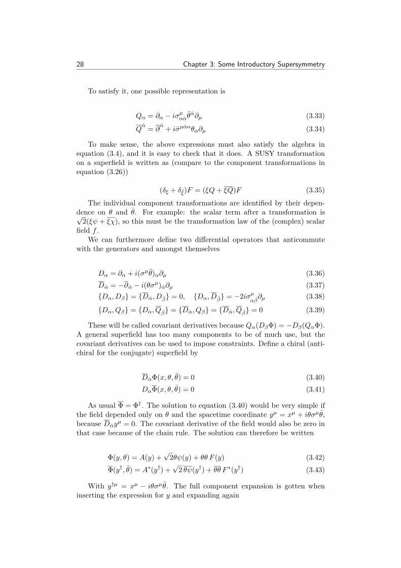
To satisfy it, one possible representation is
Qα = ∂α − iσµααθα∂µ (3.33)
Qα = ∂
α + iσµααθα∂µ (3.34)
To make sense, the above expressions must also satisfy the algebra inequation (3.4), and it is easy to check that it does. A SUSY transformationon a superfield is written as (compare to the component transformations inequation (3.26))
(δξ + δξ)F = (ξQ+ ξQ)F (3.35)
The individual component transformations are identified by their depen-dence on θ and θ. For example: the scalar term after a transformation is√
2(ξψ + ξχ), so this must be the transformation law of the (complex) scalarfield f .
We can furthermore define two differential operators that anticommutewith the generators and amongst themselves
Dα = ∂α + i(σµθ)α∂µ (3.36)Dα = −∂α − i(θσµ)α∂µ (3.37)Dα, Dβ = Dα, Dβ = 0, Dα, Dβ = −2iσµ
αβ∂µ (3.38)
Dα, Qβ = Dα, Qβ = Dα, Qβ = Dα, Qβ = 0 (3.39)
These will be called covariant derivatives because Qα(DβΦ) = −Dβ(QαΦ).A general superfield has too many components to be of much use, but thecovariant derivatives can be used to impose constraints. Define a chiral (anti-chiral for the conjugate) superfield by
DαΦ(x, θ, θ) = 0 (3.40)DαΦ(x, θ, θ) = 0 (3.41)
As usual Φ = Φ†. The solution to equation (3.40) would be very simple ifthe field depended only on θ and the spacetime coordinate yµ = xµ + iθσµθ,because Dαy
µ = 0. The covariant derivative of the field would also be zero inthat case because of the chain rule. The solution can therefore be written
Φ(y, θ) = A(y) +√
2θψ(y) + θθ F (y) (3.42)Φ(y†, θ) = A∗(y†) +
√2 θψ(y†) + θθ F ∗(y†) (3.43)
With y†µ = xµ − iθσµθ. The full component expansion is gotten wheninserting the expression for y and expanding again

3.2 The Superfield Formalism 29
Φ(x, θ, θ) = A(x) + iθσµθ∂µA(x) + 14θθ θθ ∂µ∂µA(x) +
√2θψ(x)
+ i√2θθ ∂µψ(x)σµθ + θθ F (x) (3.44)
Φ(x, θ, θ) = A∗(x) − iθσµθ∂µA∗(x) + 1
4θθ θθ ∂µ∂µA
∗(x) +√
2θψ(x)
+ i√2θθ θσµ∂µψ(x) + θθ F ∗(x) (3.45)
The highest component in Φ is the auxiliary field F and the rest are space-time derivatives. Therefore F must transform into a total derivative under aSUSY transformation
(δξ + δξ)F = i√
2∂µψσµξ (3.46)
This will be useful when constructing an action later on. Doing things bycomponents necessarily gets messy, simply because of the number of terms thathave to be included for a consistent theory. The point of having superfieldsis that they contain essentially the same information, but in a much morecompact notation. A very convenient definition is
Φ|θ=θ=0 = A(x) (3.47)DαΦ|θ=θ=0 = ψα(x) (3.48)
D2Φ∣∣∣θ=θ=0
= F (x) (3.49)
The normalization of the fields in these two points of view is not the same3,but it makes no difference which definition is chosen if the conventions arefollowed.
Another superfield that needs to be mentioned is the vector superfield,defined by the reality condition
V (x, θ, θ) = V †(x, θ, θ) (3.50)
The expansion in component fields is
V (x, θ, θ) = C(x) + iθχ(x) − iθχ(x) + i
2θθ (M(x) + iN(x)) − i
2θθ (M(x)
− iN(x)) − θσµθvµ(x) + iθθ θ
(λ(x) + i
2σµ∂µχ(x)
)− iθθ θ
(λ(x) + i
2σµ∂µχ(x)
)+ 1
2θθ θθ
(D(x) + 1
2∂µ∂µC(x)
)(3.51)
3To converge with the notation in [14], the rhs of equation (3.48) needs to be multipliedby 1√
2 and similarly in equation (3.49) a factor 14 .

30 Chapter 3: Some Introductory Supersymmetry
With C, D, M, N all real. Note that under a SUSY transformation theD-field will transform as a total derivative
(δξ + δξ)D = −12
[ξσµ∂µλ+ ∂µλσ
µξ − i
2∂µ∂νχσ
ν σµξ − i
2∂µ∂νχσ
νσµξ
](3.52)
The number of component fields can be reduced considerably by notingthat the combination Φ+Φ is a vector superfield. This can be seen as a gaugetransformation (because vµ transforms as v′
µ → vµ+i∂µΛ) and all componentsexcept λα, D and vµ can be set to zero. Therefore V can be divided into parts:V = VWZ + Φ + Φ, where
VWZ = −θσµθvµ + iθθ θλ(x) − iθθ θλ(x) + 12θθ θθ D(x) (3.53)
This is called Wess-Zumino gauge. The field, however, does not respectSUSY transformations since it has too few components to give the correctrelations. Let us use it to define two particular chiral superfields, the left- andright-handed spinor superfields
Wα = −14DDDαVWZ , W α = −1
4DDDαVWZ (3.54)
Wα is naturally chiral (W α anti-chiral), since DαDβDγ = 0 because ofanticommutivity, and furthermore
DDDαV = DDDα(VWZ + Φ + Φ) = DDDαVWZ (3.55)
The component expansion is given, in functions of the bosonic coordinatesy and y†, by
Wα = −iλα(y) + θαD(y) − i
2(σµσνθ)α(∂µvν(y) − ∂νvµ(y))
+ θθ (σµ∂µλ(y))α (3.56)
W α = iλα(y†) + θαD(y†) + i
2(σµσν θ)α(∂µvν(y†) − ∂νvµ(y†))
+ ϵαβθθ σµβα∂µλα(y†) (3.57)
There is also a reality constraint DαWα = DαWα. These fields respect
SUSY transformations and include a vector, which means that they may beused to describe gauge fields.
The next question is how to use the new tools to construct Lagrangiansand actions. For an arbitrary number of chiral superfields the most general,supersymmetrically invariant action is
S =∫d4x
[∫d4θK(Φi,Φj) +
(∫d2θW (Φi) + c.c
)](3.58)
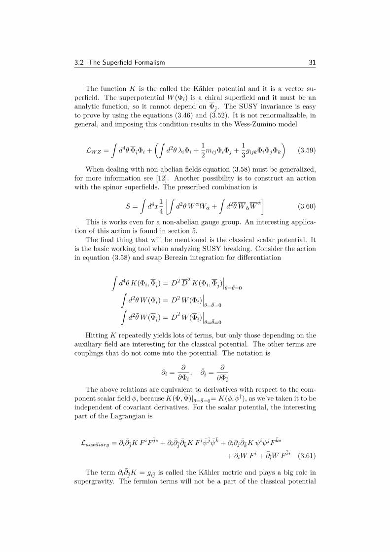
3.2 The Superfield Formalism 31
The function K is the called the Kahler potential and it is a vector su-perfield. The superpotential W (Φi) is a chiral superfield and it must be ananalytic function, so it cannot depend on Φj . The SUSY invariance is easyto prove by using the equations (3.46) and (3.52). It is not renormalizable, ingeneral, and imposing this condition results in the Wess-Zumino model
LWZ =∫d4θΦiΦi +
(∫d2θ λiΦi + 1
2mijΦiΦj + 1
3gijkΦiΦjΦk
)(3.59)
When dealing with non-abelian fields equation (3.58) must be generalized,for more information see [12]. Another possibility is to construct an actionwith the spinor superfields. The prescribed combination is
S =∫d4x
14
[∫d2θWαWα +
∫d2θW αW
α]
(3.60)
This is works even for a non-abelian gauge group. An interesting applica-tion of this action is found in section 5.
The final thing that will be mentioned is the classical scalar potential. Itis the basic working tool when analyzing SUSY breaking. Consider the actionin equation (3.58) and swap Berezin integration for differentiation
∫d4θK(Φi,Φi) = D2D
2K(Φi,Φj)
∣∣∣θ=θ=0∫
d2θW (Φi) = D2W (Φi)∣∣∣θ=θ=0∫
d2θ W (Φi) = D2W (Φi)
∣∣∣θ=θ=0
Hitting K repeatedly yields lots of terms, but only those depending on theauxiliary field are interesting for the classical potential. The other terms arecouplings that do not come into the potential. The notation is
∂i = ∂
∂Φi, ∂i = ∂
∂Φi
The above relations are equivalent to derivatives with respect to the com-ponent scalar field ϕ, because K(Φ,Φ)|θ=θ=0= K(ϕ, ϕ†), as we’ve taken it to beindependent of covariant derivatives. For the scalar potential, the interestingpart of the Lagrangian is
Lauxiliary = ∂i∂jK F iF j∗ + ∂i∂j ∂kK F iψjψk + ∂i∂j ∂kK ψiψjF k∗
+ ∂iW F i + ∂iW F i∗ (3.61)
The term ∂i∂jK = gij is called the Kahler metric and plays a big role insupergravity. The fermion terms will not be a part of the classical potential

32 Chapter 3: Some Introductory Supersymmetry
and we can neglect them. The auxiliary field can be solved for by the normalprocedure of functional derivatives. The classical potential is defined as
V = −gijFj∗F i = gij∂iW∂jW (3.62)
With this final piece of the puzzle we can at last begin to use this newformalism.

4A SUSY Breaking Sector
The first thing a phenomenologist would want to do with a brand new sym-metry, is to build an extended version of the standard model and this hasbeen done, see [1] or [2]. The Lagrangian of the MSSM was first written downusing component fields and the result is rather long, but with the superfieldformulation it is much more compact.
It is certainly encouraging to know that it is possible to construct a su-persymmetric extension of the standard model, but there are a great manythings that need a more detailed analysis. Here we will be interested in su-persymmetry breaking, in other words, explaining how and why the standardmodel particles and their supersymmetric partners have different masses. Fora deeper review see [16] and [17], while more phenomenological arguments canbe found in [1] or [18].
4.1 A SUSY Breaking Model
In section 3.1 it was briefly commented that, because the SUSY generatorscommute with P 2, the masses of both the particle and its supersymmetricpartner are the same. This is trivial to show
P 2|ϕ⟩ = m2|ϕ⟩ ⇒ P 2 (Qα|ϕ⟩) = QαP2|ϕ⟩ = m2 (Qα|ϕ⟩) (4.1)
From a phenomenological point of view this is obviously wrong. In thatcase supersymmetry would have been discovered long ago and the superpart-ners would have been found at the same time the standard model particleswere. This was not the case and that implies that supersymmetry is not anexact symmetry, but must somehow be broken. Theoretically we would like itto be spontaneously broken, which means that when the fields get their vac-uum expectation values (vev) the Lagrangian is still invariant but the ground
33
34 Chapter 4: A SUSY Breaking Sector
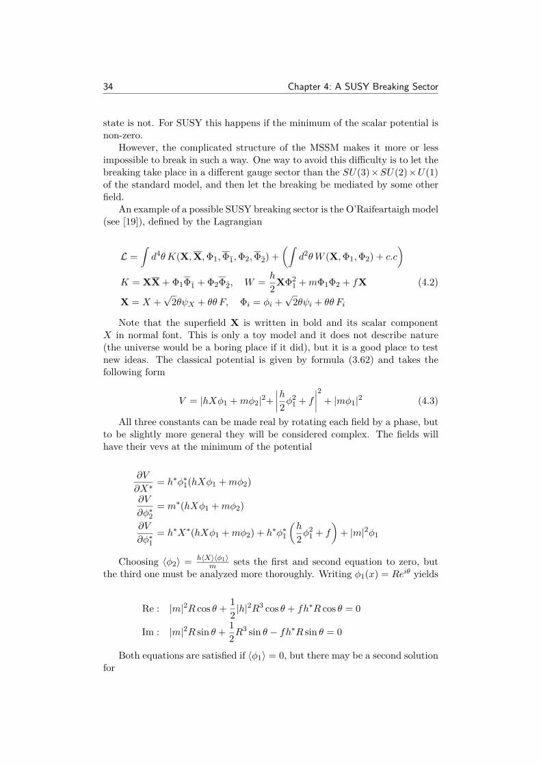
state is not. For SUSY this happens if the minimum of the scalar potential isnon-zero.
However, the complicated structure of the MSSM makes it more or lessimpossible to break in such a way. One way to avoid this difficulty is to let thebreaking take place in a different gauge sector than the SU(3)×SU(2)×U(1)of the standard model, and then let the breaking be mediated by some otherfield.
An example of a possible SUSY breaking sector is the O’Raifeartaigh model(see [19]), defined by the Lagrangian
L =∫d4θK(X,X,Φ1,Φ1,Φ2,Φ2) +
(∫d2θW (X,Φ1,Φ2) + c.c
)K = XX + Φ1Φ1 + Φ2Φ2, W = h
2XΦ2
1 +mΦ1Φ2 + fX (4.2)
X = X +√
2θψX + θθ F, Φi = ϕi +√
2θψi + θθ Fi
Note that the superfield X is written in bold and its scalar componentX in normal font. This is only a toy model and it does not describe nature(the universe would be a boring place if it did), but it is a good place to testnew ideas. The classical potential is given by formula (3.62) and takes thefollowing form
V = |hXϕ1 +mϕ2|2+∣∣∣∣h2ϕ2
1 + f
∣∣∣∣2 + |mϕ1|2 (4.3)
All three constants can be made real by rotating each field by a phase, butto be slightly more general they will be considered complex. The fields willhave their vevs at the minimum of the potential
∂V
∂X∗ = h∗ϕ∗1(hXϕ1 +mϕ2)
∂V
∂ϕ∗2
= m∗(hXϕ1 +mϕ2)
∂V
∂ϕ∗1
= h∗X∗(hXϕ1 +mϕ2) + h∗ϕ∗1
(h
2ϕ2
1 + f
)+ |m|2ϕ1
Choosing ⟨ϕ2⟩ = h⟨X⟩⟨ϕ1⟩m sets the first and second equation to zero, but
the third one must be analyzed more thoroughly. Writing ϕ1(x) = Reiθ yields
Re : |m|2R cos θ + 12
|h|2R3 cos θ + fh∗R cos θ = 0
Im : |m|2R sin θ + 12R3 sin θ − fh∗R sin θ = 0
Both equations are satisfied if ⟨ϕ1⟩ = 0, but there may be a second solutionfor

4.1 A SUSY Breaking Model 35
θ = ±π
2, R2 = 2
|h|2(fh∗ − |m|2)
This is only possible if the dimensionless parameter ξ = fh∗
|m|2 > 1, in whichcase there will be two different branches of SUSY breaking vacua. Here wewill only be interested in the case ξ < 1, and the potential is minimal when
⟨ϕ1⟩ = ⟨ϕ2⟩ = 0, ⟨X⟩ arbitrary ⇒ Vmin = |f |2 (4.4)There is no constraint for ⟨X⟩ and SUSY will be broken regardless of its
value. The degeneracy is lifted when quantum effects are considered (firstorder loop corrections) and that is the reason why we refer to X as the pseu-domodulus.
Next up is to compute the spectrum of the theory, i.e the masses of theparticles. To find the scalar masses, let the fields take their vev plus some smallquantum fluctuation ϕi(x) → ⟨ϕi⟩ + φi(x). Expand the classical potential tosecond order in φi, and gather the couplings into a matrix. The potential isgiven in terms of the superfields, so the easiest way to get the matrix is tocompute the Hessian and arrange it to be Hermitian
M2b =
∂φ1∂φ1V ∂φ1∂φ1V ∂φ1∂φ2V ∂φ1∂φ2V∂φ1∂φ1V ∂φ1∂φ1V ∂φ1∂φ2V ∂φ1∂φ2V∂φ2∂φ1V ∂φ1∂φ1V ∂φ2∂φ2V ∂φ2∂φ2V∂φ2∂φ1V ∂φ2∂φ1V ∂φ2∂φ2V ∂φ2∂φ2V
To get the masses the matrix must be diagonalized. For convenience, define
a second dimensionless parameter x = h⟨X⟩/m∗. The eigenvalues are
m2b1,b2 = |m|2
2
(2 + |x|2+|ξ|±
√4|x|2+|x|4+|ξ|2+2|ξ||x|2
)(4.5)
m2b3,b4 = |m|2
2
(2 + |x|2−|ξ|±
√4|x|2+|x|4+|ξ|2−2|ξ||x|2
)(4.6)
m2X,X
= 0
There are two bosonic masses for each field, corresponding to the two de-grees of freedom from one complex scalar field. The fermion masses are easierto compute as the mass matrix can be gotten straight from the superpotential,without having to go all the way around the classical potential.
Mf =(
∂2Φ1W (Φi) ∂Φ1∂Φ2W (Φi)
∂Φ1∂Φ2W (Φi) ∂2Φ2W (Φi)
)(4.7)
Diagonalizing gives the following eigenvalues
m2f1,f2 = |m|2
2
(|x|2+2 ±
√|x|4+4|x|2
)(4.8)
m2ψX
= 0
36 Chapter 4: A SUSY Breaking Sector
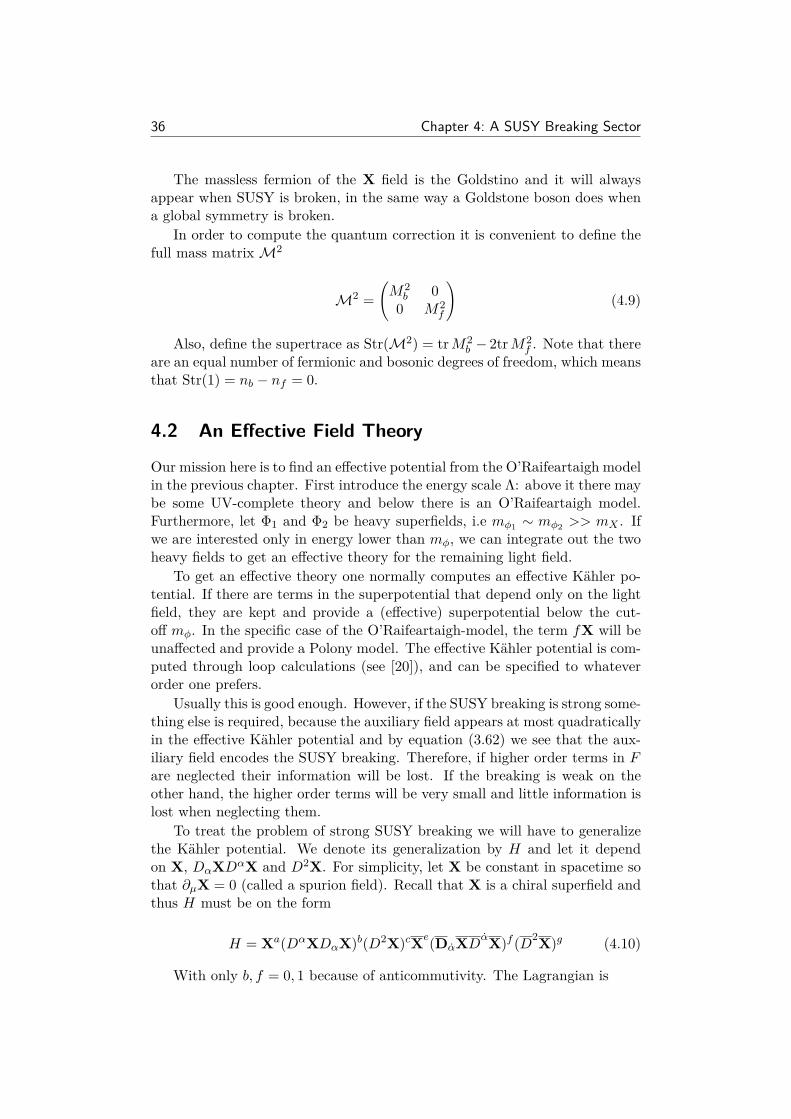
The massless fermion of the X field is the Goldstino and it will alwaysappear when SUSY is broken, in the same way a Goldstone boson does whena global symmetry is broken.
In order to compute the quantum correction it is convenient to define thefull mass matrix M2
M2 =(M2b 0
0 M2f
)(4.9)
Also, define the supertrace as Str(M2) = trM2b − 2trM2
f . Note that thereare an equal number of fermionic and bosonic degrees of freedom, which meansthat Str(1) = nb − nf = 0.
4.2 An Effective Field Theory
Our mission here is to find an effective potential from the O’Raifeartaigh modelin the previous chapter. First introduce the energy scale Λ: above it there maybe some UV-complete theory and below there is an O’Raifeartaigh model.Furthermore, let Φ1 and Φ2 be heavy superfields, i.e mϕ1 ∼ mϕ2 >> mX . Ifwe are interested only in energy lower than mϕ, we can integrate out the twoheavy fields to get an effective theory for the remaining light field.
To get an effective theory one normally computes an effective Kahler po-tential. If there are terms in the superpotential that depend only on the lightfield, they are kept and provide a (effective) superpotential below the cut-off mϕ. In the specific case of the O’Raifeartaigh-model, the term fX will beunaffected and provide a Polony model. The effective Kahler potential is com-puted through loop calculations (see [20]), and can be specified to whateverorder one prefers.
Usually this is good enough. However, if the SUSY breaking is strong some-thing else is required, because the auxiliary field appears at most quadraticallyin the effective Kahler potential and by equation (3.62) we see that the aux-iliary field encodes the SUSY breaking. Therefore, if higher order terms in Fare neglected their information will be lost. If the breaking is weak on theother hand, the higher order terms will be very small and little information islost when neglecting them.
To treat the problem of strong SUSY breaking we will have to generalizethe Kahler potential. We denote its generalization by H and let it dependon X, DαXDαX and D2X. For simplicity, let X be constant in spacetime sothat ∂µX = 0 (called a spurion field). Recall that X is a chiral superfield andthus H must be on the form
H = Xa(DαXDαX)b(D2X)cXe(DαXDαX)f (D2X)g (4.10)
With only b, f = 0, 1 because of anticommutivity. The Lagrangian is

4.2 An Effective Field Theory 37
L =∫d4 θH(X,X, DαX, DαX, D2X, D2X) +
(∫d2θ fX + c.c
)(4.11)
The DαXDαX-term (likewise for the conjugate) can be removed becauseintegration by parts yields
Dα(Xa+1DαX(D2X)cXe(DαXDαX)f (D2X)g
)= (a+ 1)Xa(DαXDαX)b(D2X)cXe(DαXDαX)f (D2X)g (4.12)
+ Xa+1(D2X)c+1Xe(DαXDαX)f (D2X)g
The lhs is zero when it is hit by D2. This will always be the case since wewill deal with H only through the Lagrangian. Thus the generalized Kahlerpotential can be chosen with b = f = 0 in equation (4.10).
The bosonic part of the action is gotten as usual but with some extradifficulty
S =∫d4x [∂X∂XHFF
∗ + fX + f∗X∗] (4.13)
Here H is a function not only of X but also of F , so when solving for theauxiliary field the equation is more complicated than usual
F (1 + F ∗∂F ∗)∂X∂XH + f∗ = 0 (4.14)
Likewise for the conjugate. Putting this result back into the Lagrangiangives the classical (scalar) potential on the form
V = |f |2(1 − F∂F − F ∗∂F ∗)∂X∂XH
|1 + F∂F∂X∂XH|2(4.15)
There are also some new couplings for the Goldstino. When computingD2D
2H by brute force the new terms that appear are
Lnew = −F
2ψ2∂X∂X∂XH − F ∗
2ψ2∂X∂X∂XH + 1
4ψ2ψ2∂X∂X∂X∂XH (4.16)
For now, let us computeH to one loop for the specific case of the O’Raifeartaighmodel. One way to do it is by a path integral, see [21] for a review. Considera Lagrangian (in Euclidean space)
Lheavy = 12
(∂ϕ)2 + m
2ϕ2, m = m(X) (4.17)
Where the mass is a function of the light field X. The generating functionalis

38 Chapter 4: A SUSY Breaking Sector
∫Dϕ exp
(−1
2
∫d4x
((∂ϕ)2 +mϕ2
))= 1√
det (−∂2+m2)Λ2
(4.18)
But this can be thought of as a potential for the X-field, because it is theonly thing left after integration. Thus we can write
∫Dϕ exp
(−1
2
∫d4x
((∂ϕ)2 −mϕ2
))= exp
(∫d4xV (X)
)(4.19)
The rhs of these two equations can be identified, but the resulting expres-sions must be massaged to a sensible form. Take the logarithm of both toget ∫
d4xV (X) = −12
log[det
(−∂2 +m2
Λ2
)](4.20)
The rhs needs some interpretation. By diagonalizing the matrix the de-terminant can be reduced to the trace of the operator. This in turn must beinterpreted as
tr O = tr (⟨x| O| y⟩) =∫d4x ⟨x| O|x⟩ (4.21)
Equation (4.20) is thus∫d4xV (X) = −1
2
∫d4x
∫d4p
(2π)4 log(p2 +m2
Λ2
)(4.22)
Where we have gone over to a momentum basis to get rid of the differentialoperator. The integration over space may diverge, but it is just the volumeof space itself and should not cause too much worry. The integrands can beidentified, with the result
V (X) = −12
∫|p|≤Λ
d4p
(2π)2 log(p2 +m2
Λ2
)
= 164π2
[Λ4(
12
− log(
Λ2 +m2
Λ2
))+ Λ2m2 +m4 log
(m2
Λ2 +m2
)](4.23)
In the limit Λ >> m it simplifies to
V (X) = 164π2
[Λ4
2+ Λ2m2 +m4 log
(m2
Λ2
)](4.24)
For several heavy fields, the mass m(X) will instead be a X-dependentmatrix and it should be traced over in the final expression. It is best writtenusing the supertrace. In the end the potential becomes
4.2 An Effective Field Theory 39
V (X) = 164π2
[Λ4
2Str(1) + Λ2Str(M2) + Str
(M4 log M2
Λ2
)](4.25)
As was already noted, Str 1 = Str M2 = 0 for the O’Raifeartaigh model1.Note that to one loop only the quadratic terms in the Lagrangian are relevant.
For the O’Raifeartaigh model, the quadratic terms are the masses in equa-tions (4.5)-(4.8), but now the light field is NOT on shell and the dimensionlessconstants x = hX
m and ξ = hFm2 depend on the components themselves, not on
their vev as before. With these masses, the expression for the scalar potentialcan be computed through equation (4.25) and put equal to the generalizedKahler potential by way of equation (4.15), in which case H is specified to oneloop order as
∂X∂XH = 164π2F 2 Str M4 log M2
Λ2
= 164π2F 2
[Str M4 log |m|2
Λ2 + Str M4 log M2
|m|2
](4.26)
This is a nice result and it calls for some discussion. The point is that wehave constructed a manifestly supersymmetric, effective theory for X, evenin the regime of strong breaking. Previously one was confined to leave X onshell when this was the case, and proceed by computing the Coleman-Weinbergpotential, but then the theory is no longer manifestly invariant under a SUSYtransformation. Therefore the method presented here is superior.
To make certain that what we have done is correct, we can compare theresult in equation (4.26) to the method with an effective Kahler potentialmentioned in the beginning. To do so we have to assume that the breakingis small, i.e fh∗/|m|2<< 1, otherwise the effective Kahler potential is not thefull answer. From [17] the expression to one loop is
Keff = − 132π2 tr
(M†M log M†M
Λ2
)(4.27)
The mass matrix M = M(X) is gotten straight from the superpotentialby looking at the quadratic terms
M : W (X,Φi) = λi(X)Φi + M(X)ΦiΦj + . . . (4.28)
For the O’Raifeartaigh model it is1This is true not only in the specific case of the O’Raifeartaigh model, but in general
for globally supersymmetric theories. Once again the situation is more complicated in su-pergravity and Str M2 = 2(n − 1)m2
3/2 − 2⟨RijGiGj⟩m2
3/2, where n is the number of chiralfields, Rij the Ricci tensor and G = K + log W + log W .

40 Chapter 4: A SUSY Breaking Sector
M(X) =(fX mm 0
)(4.29)
The classical potential is computed in the usual way by equation (3.62)
V = ∂XW∂XW
∂X ∂XKeff
= |f |2(1 − ∂X ∂XKeff + O(h4)) (4.30)
This matches the potential in (4.26). We could also consider our methodbut for a meta-stable model, with a high-energy superpotential on the form
W (Φ1,Φ2,X) = h
2XΦ2
1 +mΦ1Φ2 + fX + ϵm
2X2 (4.31)
This is somewhat more complicated than a normal O’Raifeartaigh model.The classical potential has a supersymmetric vacuum for ⟨X⟩ = − f
ϵm , but itgoes to infinity as ϵ goes to zero. Therefore the original vacuum should beapproximate and SUSY broken2. The end result is the same and the extracomplication adds no extra spice to the problem. There is no need for furtherdetails.
There is a different method presented in [22] which deals with the regimeof strong SUSY breaking. This method also deals with the cases where thepseudomodulus is integrated out or where there is no pseudomodulus at all,but these topics will not be disucssed.
In this method the pseudomodulus was taken to be a constrained super-field, which means
X2 = 0 (4.32)
In terms of components, this equation has the solution that the scalarcomponent is
X = −ψ2X
2F(4.33)
It looks simple but works remarkably well, however it prohibits all cou-plings between the Goldstino and the pseudomodulus since XψX ∼ (ψX)3 = 0.Therefore the terms in equation (4.16) will never appear. The conclusion isthat when one is interested specifically in how the Goldstino couples to thepseudomodulus, using a constrained superfield is not an option.
A subject that has been avoided here is the discussion of R-symmetry, aU(1)-symmetry, which can be used in spontaneous SUSY-breaking. In the
2A master thesis at Chalmers is required to discuss sustainable development and this ismy addition to that discussion. If the universe is in a meta-stable state it could, at any time,tunnel through from the approximate, SUSY breaking vacuum to the true supersymmetricvacuum at infinity, and reality would cease to exist. This certainly wouldn’t be in humanity’sbest interest, in which case it is of highest importance, for a sustainable society, to furtherinvestigate the issue.
4.2 An Effective Field Theory 41
O’Raifeartaigh model the field would transform as R(X) = R(Φ2) = 2 andR(Φ1) = 0. For a detailed discussion on how this ties to spontaneous SUSYbreaking see [23].
Although the O’Raifeartaigh model was used to specify the properties ofH in equation (4.26), the derivation is more general. The developed methodis certainly applicable to much more complicated models and it would be veryinteresting to apply it to something that describes reality better. Hopefullythat would lead to more interesting conclusions and deeper a physical insight.
5An Experimental Sign of SUSY
Breaking
In this section we will investigate if there is a chance of experimental detectionat the LHC of a specific SUSY breaking model. We will use a semi-directgauge mediation model (see [24], [25] and [26]), which means that the fieldthat mediates the SUSY breaking from the hidden sector to the messengers isnot the usual spurion chiral superfield but some other gauge field (here takento be U(1)). The messenger fields are charged under both the SM gauge groupand the hidden one. These fields mediate the breaking between the hiddensector and the MSSM.
Gauge mediation models with messengers have a very nice feature. With-out them, coupling the MSSM to the hidden sector directly forces one toinclude too many extra charged fields. Consider equation (2.53). In order tobreak SUSY dynamically a lot of new fields need to be added and each of theseprovide a correction, a possible particle that can circle the loop in figure C.1,that needs to be considered when computing the counterterms. This bumpsup the nf high enough to make the β-function too large thus introducing Lan-dau poles (i.e the running coupling constant diverges) at energies below theGUT scale.
The advantage of having messengers is that they screen the MSSM fromthe SUSY breaking fields, and the only correction that needs to be consideredis the one where the messenger itself is circling the loop. In this way Landaupoles can be avoided.
In so called ”minimal gauge mediation” the messengers acquire a mass viacoupling to a spurion chiral superfield, whereas in semi-direct gauge mediationthey have a tree level supersymmetric mass and get non supersymmetric masscorrections from couplings with the hidden gauge field.
We will assume that the messengers are very heavy, heavier than the CMenergy in the LHC (14 TeV). Therefore we may use an effective Lagrangian
42

5.1 Producing the Hidden Particles 43
M
g
g
h
h
∼
g
g
h
h
Figure 5.1: The Feynman diagram for the scattering process gg → hh. Theloop diagram to the left reduces to the simpler tree level process when themessengers are integrated out.
where they have been integrated out. Since the gauge group of the hiddensector is chosen to be U(1), the effective theory will be the similar to theEuler-Heisenberg Lagrangian of S-QED (for a derivation see [27]).
5.1 Producing the Hidden ParticlesThe effective action is Seff = S0 + Sint, where S0 are the kinetic terms (com-pare to equation (3.60))
S0 = 14
∫d4x
[(∫d2θW 2 + c.c
)+ 1
4
(∫d2θW a 2 + c.c
)](5.1)
The first part is the hidden sector kinetic energy and the second one, withthe color index, is the corresponding one for SU(3)c. The interacting partcomes from the Euler-Heisenberg Lagrangian
Sint = g2sg
2h
192π2M4
∫d4x
∫d2θd2θ
(W a 2W
2 +W 2Wa 2 + 4W aαWαW
aαW
α)
(5.2)Here we have taken the effective coupling constant to be gsgh/M2, where
gs is the strong coupling constant, gh is the interaction strength in the hiddensector and M is the mass of the messenger. The Feynman diagram for thescattering process is shown in figure 5.1.
The components of the spinor superfield Wα are given by equation (3.56),but here we will neglect the D-field because we are only interested in the vectorcomponent. Furthermore, use the gluons’ equations of motion
∂µFµν = 0∂[ρFµν] = 0 ⇒ 1
4σµν βα θβθσ
ρθ∂ρFµν = 0
Since we are interested in producing the hidden particles at the LHC, wecan neglect the gluinos1 in the incoming state and also the fermionic com-ponent in the outgoing state. The latter is a choice: we choose to look at
1This is a well-founded approximation because we want to investigate a cross section andthe LHC is, more or less, a gluon collider. If there is some other universe where people areusing gluino colliders, they would do it the other way around and neglect the gluons instead.

44 Chapter 5: An Experimental Sign of SUSY Breaking
the boson rather than its fermionic component. In the end the result will besimilar no matter which component we look at. The only parts of Wα thatcannot be neglected are
Wα = − i
4σµν β
α θβFµν , with σµναβFµν = fαβ (5.3)
W α = i
4σµν
αβθβFµν , with σµν
αβFµν = fαβ (5.4)
The action can be written in a more transparent form using the componentfields instead of the superfields
Sint = 148αsαhM4
∫d4x
(f2fa 2 + fa 2f2 + 4ffaf fa 2
)(5.5)
Note that this is not renormalizable, because the effective coupling constantgsghM2 has a dimension, it goes like [E]−2. As long as we restrict the computation
to tree level amplitudes and s << M2 (i.e the messengers circling the loop infigure 5.1 are off shell) everything is ok.
Denote the hidden field strength by Gµν . The matrix element for thescattering process is written simply as
M = −i 148αsαhM4
× ⟨p1, ε1; p2, ε2|Tµ1ν1...µ4ν4Fµ1ν1Fµ2ν2Gµ3ν3Gµ4ν4 | k1, λ1; k2, λ2⟩ (5.6)
Here p1, p2, ε1 and ε2 are the momenta and polarization vectors of thegluons and k1, k2, λ1 and λ2 the corresponding ones for the hidden particles.The tensor Tµ1ν1...µ4ν4 is gotten from the action
Tµ1ν1...µ4ν4 = tr (σµ1ν1σµ2ν2) tr (σµ3ν3 σµ4ν4) + tr (σµ3ν3σµ4ν4)× tr (σµ1ν1 σµ2ν2) + 4tr (σµ1ν1σµ3ν3) tr (σµ2ν2 σµ4ν4) (5.7)
When contracting the fields with the external states it becomes
M = −iαsαh3M4 V
µ1ν1...µ4ν4p1µ1p2µ2k1µ3k2µ4ε1 ν1ε2 ν2λ1 ν3λ2 ν4 (5.8)
V µ1ν1...µ4ν4 = Tµ1ν1...µ4ν4 + (1 ↔ 2) + (3 ↔ 4) +(
1 ↔ 23 ↔ 4
)(5.9)
The traces can be simplified by some neat identities, see [28] for reference.There is no real point in proceeding further by hand, but rather use somesoftware2 to compute it. The polarization sums were calculated using thestandard substitution
2Here the computations were performed using the Mathematica package Ricci, seehttp://www.math.washington.edu/˜lee/Ricci/ for more information.
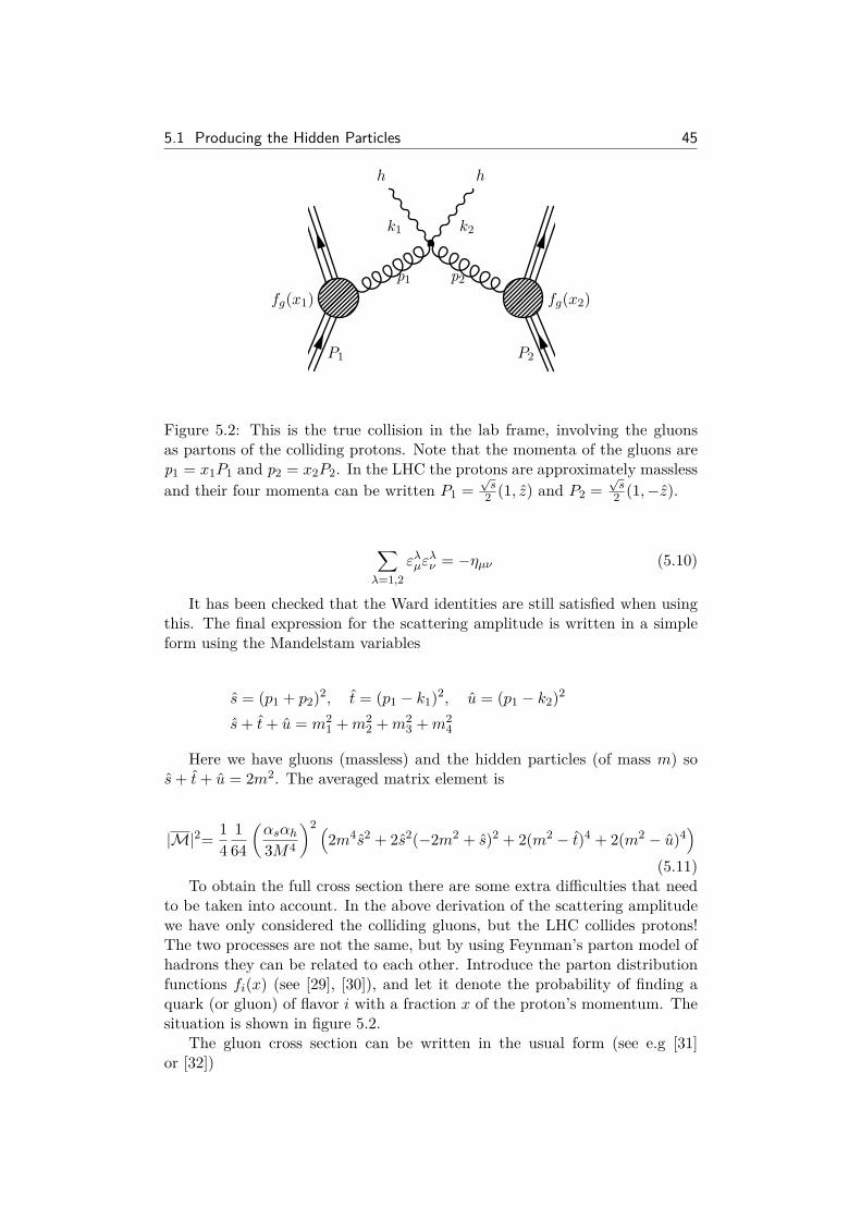
5.1 Producing the Hidden Particles 45
P1 P2
k1
p1 p2
k2
h h
fg(x1) fg(x2)
Figure 5.2: This is the true collision in the lab frame, involving the gluonsas partons of the colliding protons. Note that the momenta of the gluons arep1 = x1P1 and p2 = x2P2. In the LHC the protons are approximately masslessand their four momenta can be written P1 =
√s
2 (1, z) and P2 =√s
2 (1,−z).
∑λ=1,2
ελµελν = −ηµν (5.10)
It has been checked that the Ward identities are still satisfied when usingthis. The final expression for the scattering amplitude is written in a simpleform using the Mandelstam variables
s = (p1 + p2)2, t = (p1 − k1)2, u = (p1 − k2)2
s+ t+ u = m21 +m2
2 +m23 +m2
4
Here we have gluons (massless) and the hidden particles (of mass m) sos+ t+ u = 2m2. The averaged matrix element is
|M|2= 14
164
(αsαh3M4
)2 (2m4s2 + 2s2(−2m2 + s)2 + 2(m2 − t)4 + 2(m2 − u)4
)(5.11)
To obtain the full cross section there are some extra difficulties that needto be taken into account. In the above derivation of the scattering amplitudewe have only considered the colliding gluons, but the LHC collides protons!The two processes are not the same, but by using Feynman’s parton model ofhadrons they can be related to each other. Introduce the parton distributionfunctions fi(x) (see [29], [30]), and let it denote the probability of finding aquark (or gluon) of flavor i with a fraction x of the proton’s momentum. Thesituation is shown in figure 5.2.
The gluon cross section can be written in the usual form (see e.g [31]or [32])

46 Chapter 5: An Experimental Sign of SUSY Breaking
dσij = 12s
|M|2dLips2 (5.12)
dLipsn =(
n∏i
d3ki(2π)3
12Ei
)δ4(pin −
n∑i
ki) (5.13)
Using Lorentz invariance, the two integrals coming from dLips2 can becomputed in the center of mass frame of the gluons3, and the differential crosssection written
dσij
dt= |M|2
16πs2 , t± = m2 − s
2
1 ±
√1 − 4m2
s
(5.14)
Introduce another factor 1/2 (because the outgoing particles are identical)and integrate between t− and t+ to get the full cross section for the gluoncollision
σij = 1128
(αsαh
3
)2 s3
40πM8
√1 − 4m2
s
(27m
4
s2 − 26m2
s+ 7
)(5.15)
The cross section for the protons is gotten when summing up all possibleparton configurations. With the previously introduced PDFs4 this is simplydone by including them and integrating over the fraction of momenta carriedby the gluons
σ =∫ 1
0dx1
∫ 1
0dx2
∑i,j
fi(x1)fj(x2)σij (5.16)
Here∑fi(x1)fj(x2) = fg(x1)fg(x2). The integration is done numerically
and the process is plotted versus the hidden particle mass in figure 5.3, withM = 1 TeV/c2, αh = αs = 0.069 and s = 14 TeV. Equation (5.15) can be usedto get σ for any value of M or αh.
Unfortunately the cross section is very small. A good landmark for com-parison is to use an integrated luminosity of one inverse femtobarn to estimatethe number of events, which is simply the integrated luminosity times the crosssection. For this process we would have approximately 0.07 events, i.e noneat all.
Furthermore, the messenger mass was taken rather low: it is expected tobe much bigger and since the equation (5.15) goes like M−8, a small increase
3This is a very nice simplification, otherwise one would have to compute the integrals inthe lab frame. In this case it is the same as the CM frame of the protons, where p1 = p2 andthere would be x1 and x2 everywhere. In the end, this way of doing things must of coursegive the same answer and it has been checked that it does.
4Numerical values for the PDFs are based on measurements form the Hera experimentand it was taken from http://hepdata.cedar.ac.uk/pdf/pdf3.html.
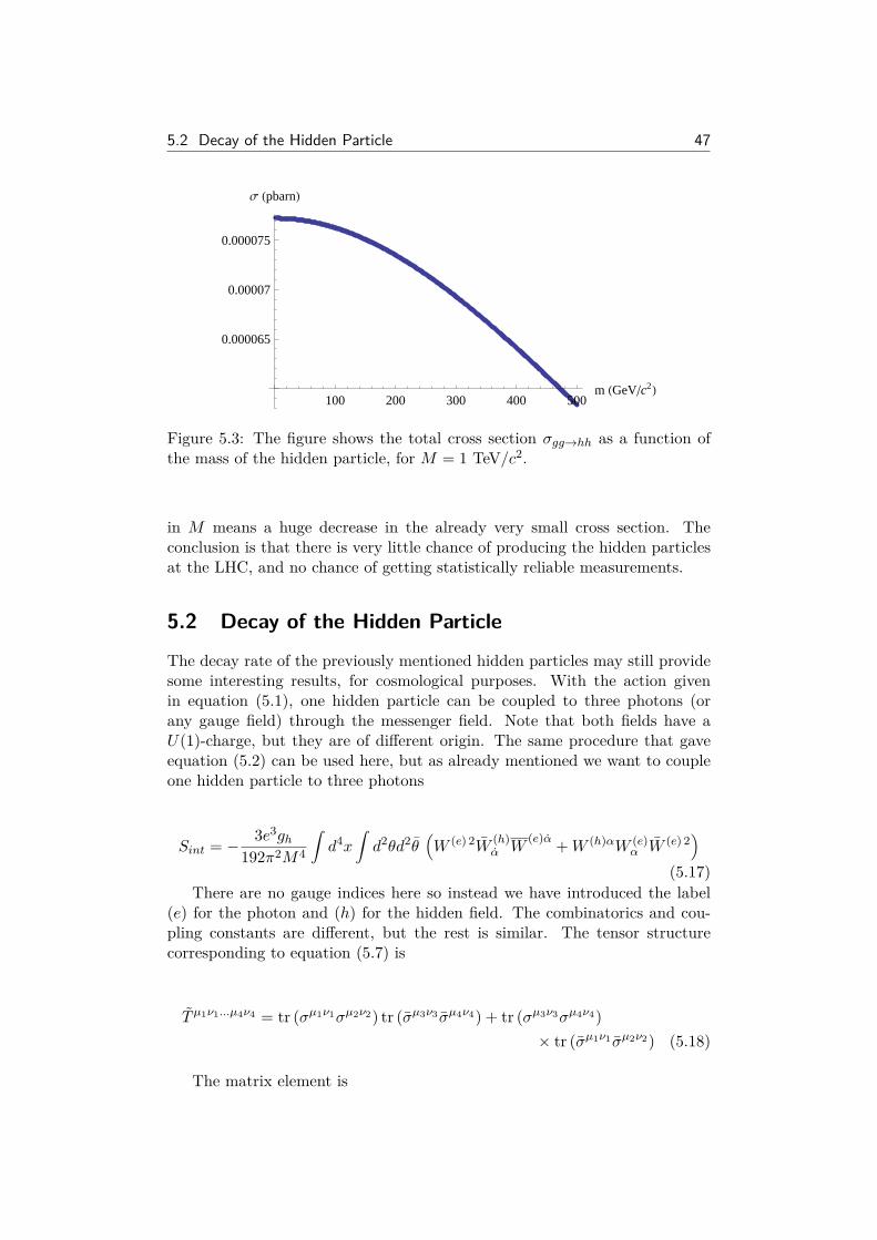
5.2 Decay of the Hidden Particle 47
100 200 300 400 500m HGeVc2L
0.000065
0.00007
0.000075
Σ HpbarnL
Figure 5.3: The figure shows the total cross section σgg→hh as a function ofthe mass of the hidden particle, for M = 1 TeV/c2.
in M means a huge decrease in the already very small cross section. Theconclusion is that there is very little chance of producing the hidden particlesat the LHC, and no chance of getting statistically reliable measurements.
5.2 Decay of the Hidden Particle
The decay rate of the previously mentioned hidden particles may still providesome interesting results, for cosmological purposes. With the action givenin equation (5.1), one hidden particle can be coupled to three photons (orany gauge field) through the messenger field. Note that both fields have aU(1)-charge, but they are of different origin. The same procedure that gaveequation (5.2) can be used here, but as already mentioned we want to coupleone hidden particle to three photons
Sint = − 3e3gh192π2M4
∫d4x
∫d2θd2θ
(W (e) 2W
(h)α W
(e)α +W (h)αW (e)α W (e) 2
)(5.17)
There are no gauge indices here so instead we have introduced the label(e) for the photon and (h) for the hidden field. The combinatorics and cou-pling constants are different, but the rest is similar. The tensor structurecorresponding to equation (5.7) is
Tµ1ν1...µ4ν4 = tr (σµ1ν1σµ2ν2) tr (σµ3ν3 σµ4ν4) + tr (σµ3ν3σµ4ν4)× tr (σµ1ν1 σµ2ν2) (5.18)
The matrix element is

48 Chapter 5: An Experimental Sign of SUSY Breaking
M = e3gh(4π)2M4B
µ1ν1...µ4ν4pµ1λν1k1µ2ε1 ν2k2µ3ε2 ν3k3µ4ε3 ν4 (5.19)
Bµ1ν1...µ4ν4 = Tµ1ν1...µ4ν4 + (all permutations of 234) (5.20)(5.21)
This is a 1 → 3 process and is thus best presented using the variables
s = (p1 − k1)2, t = (p1 − k2)2, u = (p1 − k3)2 (5.22)s+ t+ u = m2 +m2
1 +m22 +m2
3 (5.23)
Here the decay products are photons so m1 = m2 = m3 = 0. The sameprocedure for the sum over polarization is used here, but the hidden particlecan have three different polarizations
|M|2= 13
∑polarizations
|M|2= α3eαh
6M8
(s4 + t4 + u4 − 2m2(s3 + t3 + u3)
+m4(s2 + t2 + u2))
= α3eαh
6M8 g(s, t, u) (5.24)
The expression for the differential decay rate can be found in e.g [3]
dΓ(1 → 3) = 12m
|M|2dLips3 (5.25)
The kinematic integrals in the massless case turn out to be
dLips3 = 13!
116(2π)3
ds dt
m2 , s, t ∈ [0,m2] (5.26)
The extra factor of 13! is there to avoid counting identical configurations
several times, because the three decay products are identical particles. Thedecay rate can be computed in closed form
Γ = α3eαh
1152(2π)3m3M8
∫ds dt g(s, t,m2 − s− t) = α3
eαh30720π3
m9
M8 (5.27)
This can be plotted but it is more informative to plot its inverse τ = 1/Γ,with τ the mean life time, shown in figure 5.4.
We see that the decay rate can vary over many orders of magnitude. Notethat if the hidden particle exist, lots of them would have been created at theBig Bang. With a more likely value for the messenger mass, say M = 10TeV, the mean life time of the hidden particle can, depending on its mass, begreater than the age of the universe (roughly 1019 s). This means that mostof it would still be around, providing a possible candidate for dark matter.

5.2 Decay of the Hidden Particle 49
100 200 300 400 500m HGeVL
1
1000
106
109
1012
Τ HsL
Figure 5.4: Logarithmic plot of the mean life time of the process h → γγγ,with M = 1 TeV/c2 and αh = αs. There are several other decay channels (e.gh → ggg or h → ggg) and τ is therefore smaller, but the order of magnitudeshould be correct.
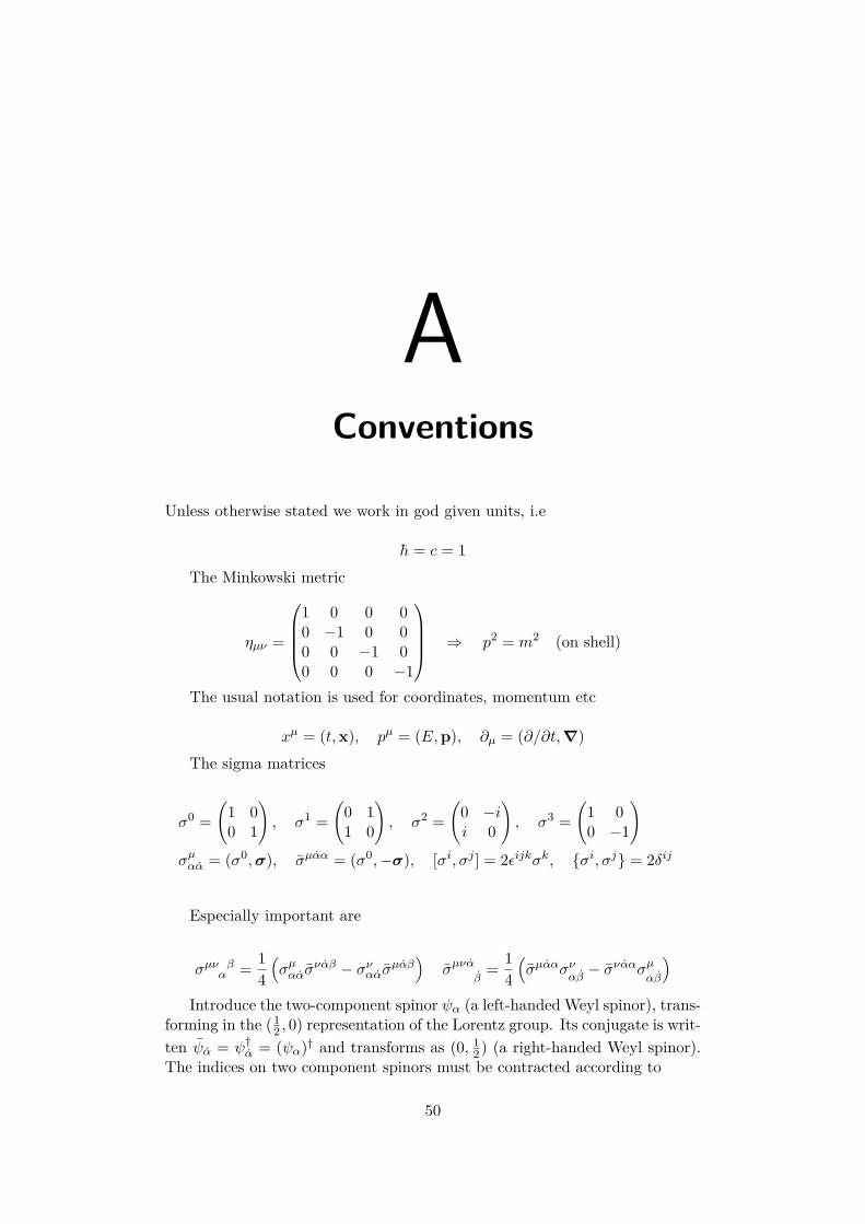
AConventions
Unless otherwise stated we work in god given units, i.e
h = c = 1The Minkowski metric
ηµν =
1 0 0 00 −1 0 00 0 −1 00 0 0 −1
⇒ p2 = m2 (on shell)
The usual notation is used for coordinates, momentum etc
xµ = (t,x), pµ = (E,p), ∂µ = (∂/∂t,∇)The sigma matrices
σ0 =(
1 00 1
), σ1 =
(0 11 0
), σ2 =
(0 −ii 0
), σ3 =
(1 00 −1
)σµαα = (σ0,σ), σµαα = (σ0,−σ), [σi, σj ] = 2ϵijkσk, σi, σj = 2δij
Especially important are
σµν βα = 1
4
(σµαασ
ναβ − σναασµαβ
)σµνα
β= 1
4
(σµαασν
αβ− σναασµ
αβ
)Introduce the two-component spinor ψα (a left-handed Weyl spinor), trans-
forming in the (12 , 0) representation of the Lorentz group. Its conjugate is writ-
ten ψα = ψ†α = (ψα)† and transforms as (0, 1
2) (a right-handed Weyl spinor).The indices on two component spinors must be contracted according to
50

51
ξζ = ξαζα = ξαζβϵαβ , λρ = λαρα = λαρβϵ
αβ, λα = (λα)†
ϵαβ =(
0 1−1 0
), ϵαβ =
(0 −11 0
), ϵαβ = (ϵαβ)∗
Suppressed indices can always be reconstructed with these conventions,for example: ψσµχ = ψασµααχ
α. For a wealth of identities for two componentspinors see [28].
A chiral representation is used for the 4-component Dirac spinors, wherethe gamma-matrices are
γµ =(
0 σµ
σµ 0
), γµ, γν = 2ηµν (A.1)
Note that with this representation we can write a Dirac spinor as
ΨD =(ψαξα
)(A.2)
Important integrals
∫ddℓ
(2π)d1
(ℓ2 − ∆)n= (−1)n
(4π)d/2Γ(n− d/2)
Γ(n)
( 1∆
)n−d/2(A.3)∫
ddℓ
(2π)dℓ2
(ℓ2 − ∆)n= (−1)n−1
(4π)d/2id
2Γ(n− d/2 − 1)
Γ(n)
( 1∆
)n−d/2−1(A.4)

BGhosts
In section 2.2 it was briefly mentioned that the Yang-Mills Lagrangian inequation (2.7) is not quite the full story . To quantize it we will use themethod of path integrals. Ignore the fermions and consider only the gluonfield in the generating functional
Z =∫
DAµ e−SYM [Aµ] (B.1)
In the action a Wick rotation has been made (x0 → ix0) to get an Euclideanmetric and the minus sign. Along some directions of Aµ the action SYM willbe constant, because it is invariant under gauge transformation. Thereforewhen we try to compute the vacuum energy ⟨0|0⟩ and integrate over all paths,we will get an infinite result along those directions. Such a divergence mustbe treated somehow, but it is not of the same type as those that appear inrenormalization and cannot be removed in the same way. The way to handleit was proposed by Faddeev and Popov (see [33]) and the resulting Lagrangianis called the Faddeev-Popov Lagrangian.
To start out we make a naive analogy: the situation is similar to a normaldouble integral with the integrand only depending on one of the directions
Z =∫dx dy e−S[x] → ∞ (B.2)
Such a problem could be avoided in a number of ways. The most obviousis to skip the integration in y, but that would be very difficult to do for apath integral. Another possibility is to insert a delta function δ(y). Thiswould certainly work for a functional measure and to make it more generalwe insert δ(f(x, y)), such that f(x, y) = 0 for some path y(x). The functionf(x, y) defines a gauge fixing along all possible gauge orbits, and the changeof variables in the delta function brings about the Jacobian (∂f/∂y|x). Themodified integral is
52

53
Z =∫dx dy
∂f
∂y
∣∣∣∣x
δ(f(x, y))e−S[x] (B.3)
Consider now the multidimensional generalization
Z =∫dnX dmY det
(∂fa
∂Y b
) m∏c=1
δ(f c(X,Y ))e−SYM [X] (B.4)
The f c(X,Y ) fixes the gauge in m directions. The determinant can beinterpreted as a functional determinant, coming from a fermionic field
det(∂fa
∂Y b
)=∫dmη dmη exp[−ηa
∂fa
∂Y bηb] (B.5)
The η is called a BRST-ghost. Likewise, the delta function can be rewrittenas an integral
∏δ(f c(X,Y )) =
∫dmB e−iBcfc(X,Y ) (B.6)
With these new fields the full path integral is
Z =∫dnX dmY dmη dmη dmB exp
(−SYM [X] − η
∂f
∂Yη − iBT f(X,Y )
)(B.7)
The linear term is unphysical (it is a tadpole), but we can modify theintegral by including a quadratic term ξ
2B2 and complete the square, then
integrate the B-fields away. The modification only changes the constant infront of the integral and that cancels when computing correlation functions.The generating functional can be written as
Z =∫dnX dmY dmη dmη exp
(−SYM [X] − η
∂f
∂Yη + 1
2ξf †f
)(B.8)
For the Yang-Mills Lagrangian (equation (2.5)), SYM is invariant underAaµ → Aaµ+∂µΛa−gfabcAbµΛc. Some function must be chosen to fix the gaugeand, theoretically, anything would do as long as it is not gauge invariant. Inpractice we still require something that is both Lorentz invariant and linear,and the canonical choice is
fa = ∂µAµa = 0 (B.9)
Note that under a gauge transformation this condition transforms as ∂µAaµ →∂µAaµ + ∂µDab
µ Λb (with the covariant derivative defined as Dabµ = δab∂µ −
gfabcAcµ), in which case
∂fa
∂Y b= δ
δΛb(y)∂µAaµ(x) = ∂µDab
µ δ(x− y) (B.10)
54 Appendix B: Ghosts
The η-integral can be written properly with the above information and thenew field c
det(∂fa
∂Y b
)=∫
DcDc exp(∫
d4x ca∂µDabµ c
b)
(B.11)
The final form of the gauge sector in the Yang-Mills action is
SYM =∫d4x
[−1
4F aµνF
aµν − ca(∂µDabµ )cb − 1
2ξ(∂µAaµ)2
](B.12)
The end result is that a new field ca has appeared. This is not a physicalfield, it is a theoretical tool to help kill of the extra degrees of freedom comingfrom gauge invariance. However it does provide a new interaction with thegluon field and this must be taken into account in the same way as any othervertex.
The second term, 12ξ (∂µAaµ)2, is a correction to the propagator and we
have to take it into account when computing the full expression for the gluontwo-point correlation function
⟨Ω|TAaµAbν | Ω⟩ = −iδab
k2 + iϵ
(ηµν − (1 − ξ)kµkν
k2
)(B.13)
.In this thesis ξ = 1, called the Feynman-’t Hooft gauge. The physics must
be independent of ξ but depending on what is described other choices may bepreferable.
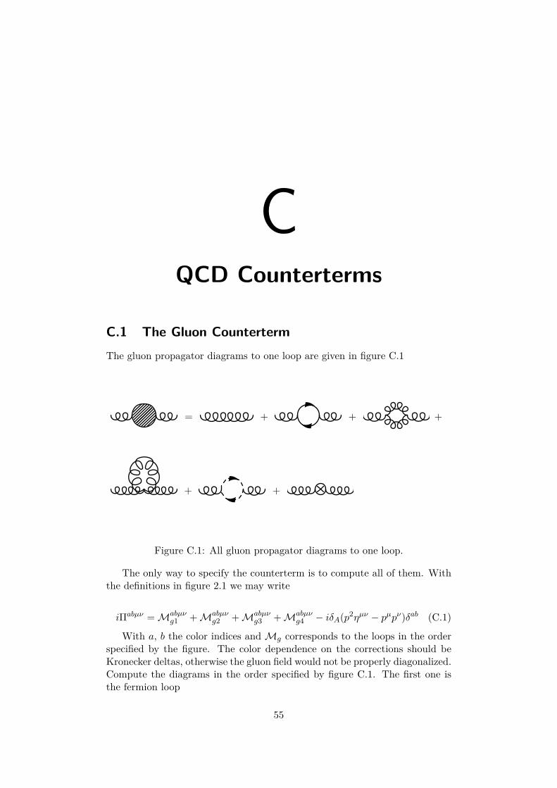
CQCD Counterterms
C.1 The Gluon CountertermThe gluon propagator diagrams to one loop are given in figure C.1
= + + +
+ +
Figure C.1: All gluon propagator diagrams to one loop.
The only way to specify the counterterm is to compute all of them. Withthe definitions in figure 2.1 we may write
iΠabµν = Mabµνg1 + Mabµν
g2 + Mabµνg3 + Mabµν
g4 − iδA(p2ηµν − pµpν)δab (C.1)
With a, b the color indices and Mg corresponds to the loops in the orderspecified by the figure. The color dependence on the corrections should beKronecker deltas, otherwise the gluon field would not be properly diagonalized.Compute the diagrams in the order specified by figure C.1. The first one isthe fermion loop
55

56 Appendix C: QCD Counterterms
p
k
p
k + p
Application of the Feynman rules gives the expression
Mabµνg1 = −tr[T aT b]
∫ddk
(2π)dtr[(igµεγµ)i
/k + /p+m
(k + p)2 −m2 + iϵ(igµεγν)
×i/k +m
k2 −m2 + iϵ
](C.2)
The first minus sign is needed because it is a fermion circling the loop. TheLie algebra factor is trT aT b and can be chosen proportional to the identitymatrix times some constant C(r)δab, different for each representation (see[11]). Remove the Kronecker delta to make the derivation cleaner. Using theFeynman parameters and shifting the momentum to ℓµ = kµ + xpµ bringsthe integral to the usual form, and all odd powers of ℓ can be dropped in thenumerator. The resulting expression is
Mµνg1 = −g2µ2εC(r)
∫ 1
0dx
∫ddℓ
(2π)dNµν
(ℓ2 − ∆)2 (C.3)
Nµν = dm2ηµν + d[2ℓµℓν − 2x(1 − x)pµpν − (ℓ2 − x(1 − x)p2)ηµν
]∆ = x(x− 1)p2 +m2 − iϵ
Inside the integral Lorentz invariance demands that ℓµℓν = Aηµνℓ2 andcontracting the indices on both sides shows A = 1/d, after which it can becomputed as before. Tables for the integrals can be found in the appendixof [3] and the result is
Mµνg1 = −ig
2µ2εC(r)(4π)d/2
∫ 1
0dx d
[(m2ηµν − x(1 − x)(2pµpν − p2ηµν)
)×Γ(2 − d/2)
∆2−d/2 − ηµν(d2
− 1)Γ(1 − d/2)∆1−d/2
](C.4)
The last term is the apparent quadratic divergence1 but if the Gammafunction is expanded we get
1It is called a quadratic divergence because it is divergent for d = 2.

C.1 The Gluon Counterterm 57
(d2
− 1)Γ(1 − d/2) = −(1 − d/2)Γ(2 − d/2)1 − d/2
(C.5)
The factor in front cancels the quadratic divergence. Combining the twocontributions (by multiplying the latter by ∆/∆) yields
Mµνg1 = i
g2µ2εC(r)(4π)d/2
(pµpν − p2ηµν
) ∫ 1
0dx 2dΓ(2 − d/2)
∆2−d/2 [x(1 − x)] (C.6)
Note that the tensor structure pµpν − p2ηµν is transverse to pµ. This isnot a coincidence but actually a requirement forced onto the propagator bythe Ward identity. The tensor part of the gluon propagator MUST be of thisform, otherwise it violates gauge invariance. Each flavor of quark contributesto this diagram so we must multiply the above result by nf .
The second diagram is
p
k
p
k + p
Application of the Feynman rules give
Mabµνg2 = −g2µ2ε
2
∫ddk
(2π)df cad [ηρµ(k − p)σ + ηµσ(2p+ k)ρ − ησρ(2k + p)µ]
× ησκδdd′
(k + p)2 + iϵfd
′bc′ [ηκν(2p+ k)λ + ηνλ(k − p)κ − ηλκ(2k + p)ν
] ηλρδcc′
k2 + iϵ(C.7)
The factor of 1/2 is a symmetry factor and needed because the gluonpropagators inside the loop are equivalent. The Lie algebra factor is theCasimir operator but for the adjoint representation, denoted by r = G, sofacdf bcd = C2(G)δab. Shift momentum to ℓµ = kµ + xpν and drop all oddpowers of ℓ
Mµνg2 = g2µ2εC2(G)
2
∫ 1
0dx
∫ddℓ
(2π)dNµν
(ℓ2 − ∆)2 (C.8)
Nµν = 6(ℓ2ηµν − ℓµℓν) + ((1 + x)2 + (2 − x)2)ηµνp2
+ pµpν((d− 2)(1 − 2x)2 − 2(1 + x)(2 − x)
)∆ = x(x− 1)p2 − iϵ

58 Appendix C: QCD Counterterms
The integration can be performed in the familiar way and the result is
Mµνg2 = ig2µ2εC2(G)
2(4π)d/2
∫ 1
0
dx
∆2−d/2 [3(1 − d)∆ηµνΓ(1 − d/2) + ΞµνΓ(2 − d/2)]
(C.9)The third diagram is
p p
k
The Feynman rules give the amplitude
Mabµνg3 = −ig
2µε
2
[f cdefabe (ηρµησν − ηρνησµ) + f caefdbe (ηρσηµν − ηρνησµ)
+f cbefdae (ηρσηµν − ηρµησν)] ∫ ddk
(2π)d−iηρσδcd
k2 + iϵ(C.10)
The factor of 1/2 is again due to symmetry. To make the amplitude looklike the ones already computed we multiply by (k + p)2/(k + p)2 and shiftmomentum. The expression simplifies to
Mµνg3 = (1 − d)g2µεC2(G)ηµν
∫ 1
0dx
∫ddℓ
(2π)dℓ2 + (1 − x)2p2
(ℓ2 − ∆)2 (C.11)
Again the color delta has been taken away. The integral solves to
Mµνg3 = i
g2C2(G)(4π)2 (1 − d)ηµν
∫ 1
0
dx
∆2−d/2
[(1 − x)2p2Γ(2 − d/2)
−d
2∆Γ(1 − d/2)
](C.12)
This does not fix the any of the problems that came up. The only hope isthe final diagram, the ghost contribution
p
k
p
k + p
C.1 The Gluon Counterterm 59
The matrix element is
Mabµνg4 = −
∫ddk
(2π)d(−gµεfdac) i(k + p)µ
(k + p)2 + iϵ(−gµεf cbd) ikν
k2 + iϵ(C.13)
The ghost are fermions which explains the extra minus sign. Shift momen-tum and simplify as before to get the expression
Mµνg4 = −g2µ2εC2(G)
∫ 1
0dx
∫ddℓ
(2π)dℓµℓν − x(1 − x)pµpν
(ℓ2 − ∆)2 (C.14)
The final form of the ghost contribution is
Mµνg4 = i
g2µ2εC2(G)(4π)2
∫ 1
0
dx
∆2−d/2 [x(1 − x)pµpνΓ(2 − d/2)
+ηµν ∆2
Γ(1 − d/2)]
(C.15)
Now we sum up the four contributions and take a closer look at the coef-ficient in front of the seemingly quadratic divergence
12
(3(1 − d) − d(1 − d) + 1) Γ(1 − d/2) = 2(
1 − d
2
)2Γ(1 − d/2)
= 2(
1 − d
2
)Γ(2 − d/2) (C.16)
It cancels! This would not have happened without the ghost diagram. Thesecond thing that needs checking is that the tensor structure has the properform. The coefficients in front of the different parts are
p2ηµν : 2x(x− 1)(1 − d/2) + (1 − d)(1 − x)2 + 12
((1 + x)2 + (2 − x)2
)pµpν : (d
2− 1)(1 − 2x)2 − 2
At first glance they do not look the same. The brute force way of showingit is to perform the integrals in x and both turn out to be ±7
3 ∓ d6 . A more
elegant way to do it is by realizing that the expression is symmetric underx → 1 − x, a consequence of the Feynman parameters, in which case we maysimplify by letting x → 1
2x+ 12(1−x) = 1
2 . For the coefficient in front of p2ηµν ,it yields
p2ηµν : −d
2
[(1 − 2x)2 + 1 − 2x
]+ (1 − 2x)2 + 2 + 1
2− x
→ −(d2
− 1)(1 − 2x)2 + 2 (C.17)

60 Appendix C: QCD Counterterms
Note that dimensional regularization is a requirement for this to work.Unlike the quark counterterm, here it would not be possible to both satisfythe Ward identities and get the correct tensor structure using a Pauli-Villarsprescription. The counterterm can now be specified by summing up the fourdiagrams and using equation (C.1) at p2 = µ2
δA = g2
16π2
∫ 1
0dx
1ε
1 + ε log
µ2
∆
∣∣∣∣∣p2=µ2
+ O(ε2)
×((2 − (1 − 2x)2)C2(G) − 8nfx(1 − x)C(r)
)](C.18)
The divergent part is
limε→0
εδA = g2
16π25C2(G) − 4nfC(r)
3(C.19)
C.2 The Vertex CountertermThe diagrams are given by figure C.2. Write the propagator as
= + + +
Figure C.2: The vertex correction diagrams to one loop.
igµεΓµDa = igγµT a + Maµv1 + Maµ
v2 + igµεδgγµT a (C.20)
The first diagram is
q
k − qk
k − p1p1 p2
Maµv1 = g3µ3εT bT aT b
∫ddk
(2π)dγρ
/k +m
k2 −m2 + iϵγµ
/k − /q +m
(k − q)2 −m2 + iϵγσ
× ησρ(k − p1)2 + iϵ
(C.21)
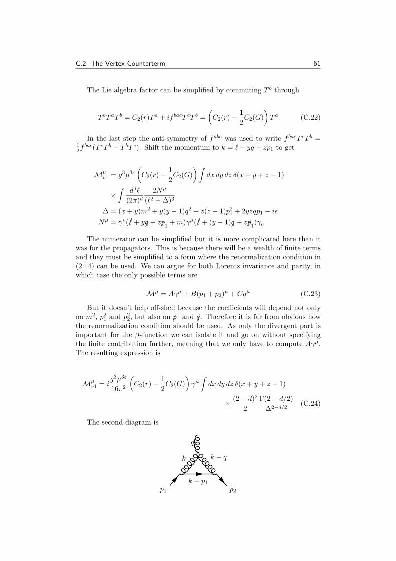
C.2 The Vertex Counterterm 61
The Lie algebra factor can be simplified by commuting T b through
T bT aT b = C2(r)T a + if bacT cT b =(C2(r) − 1
2C2(G)
)T a (C.22)
In the last step the anti-symmetry of fabc was used to write f bacT cT b =12f
bac(T cT b − T bT c). Shift the momentum to k = ℓ− yq − zp1 to get
Mµv1 = g3µ3ε
(C2(r) − 1
2C2(G)
)∫dx dy dz δ(x+ y + z − 1)
×∫
ddℓ
(2π)d2Nµ
(ℓ2 − ∆)3
∆ = (x+ y)m2 + y(y − 1)q2 + z(z − 1)p21 + 2yzqp1 − iϵ
Nµ = γρ(/ℓ + y/q + z/p1 +m)γµ(/ℓ + (y − 1)/q + z/p1)γρ
The numerator can be simplified but it is more complicated here than itwas for the propagators. This is because there will be a wealth of finite termsand they must be simplified to a form where the renormalization condition in(2.14) can be used. We can argue for both Lorentz invariance and parity, inwhich case the only possible terms are
Mµ = Aγµ +B(p1 + p2)µ + Cqµ (C.23)
But it doesn’t help off-shell because the coefficients will depend not onlyon m2, p2
1 and p22, but also on /p1 and /q. Therefore it is far from obvious how
the renormalization condition should be used. As only the divergent part isimportant for the β-function we can isolate it and go on without specifyingthe finite contribution further, meaning that we only have to compute Aγµ.The resulting expression is
Mµv1 = i
g3µ3ε
16π2
(C2(r) − 1
2C2(G)
)γµ∫dx dy dz δ(x+ y + z − 1)
× (2 − d)2
2Γ(2 − d/2)
∆2−d/2 (C.24)
The second diagram is
q
k − qk
k − p1p1 p2

62 Appendix C: QCD Counterterms
Maµv2 = ig3µ3ε
∫ddk
(2π)d[−ηµν(q + k)µ + ηνρ(2k − q)µ + ηρµ(2q − k)ν ]
× fabcT bT cγλ/k − /p1 +m
(k − p1)2 −m2 + iϵγσ
ηνλk2 + iϵ
ηρσ(k − q)2 + iϵ
(C.25)
The Lie algebra factor simplifies to i2C2(G)T a. Shift momentum to ℓ =
k − yq − zp1 and combine the denominator
Mµv2 = −g3µ3εC2(G)
2
∫dx dy dz δ(x+ y + z − 1)
∫ddℓ
(2π)22Nν
(ℓ2 − ∆)3
∆ = xm2 + y(y − 1)q2 + z(z − 1)p21 + 2yzqp1 − iϵ
Nµ = −γµ(/ℓ + y/q + (z − 1)/p1 +m)(/ℓ + (1 + y)/q + z/p1)− (/ℓ + (y − 2)/q + z/p1)(/ℓ + y/q + (z − 1)/p1 +m)γµ
+ γρ(/ℓ + y/q + (z − 1)/p1 +m)γρ(2ℓ+ (2y − 1)q + 2zp1)µ
As before we are only interested in the divergent part and it integrates to
Mµv2 = −ig
3µ3εC2(G)16π2 γµ(1−d)
∫dx dy dz δ(x+y+z−1)Γ(2 − d/2)
∆2−d/2 (C.26)
With the counterterm specified as in equation (C.20), with x = 1 − z − y
δg = −g2µ2ε
16π2
∫dy dz
1ε
1 + ε log
µ2
∆
∣∣∣∣∣p2=µ2
+ O(ε2)
× 2 (C2(r) + C2(G)) (C.27)
The divergent part is
limε→0
εδg = − g2
16π2 (C2(r) + C2(G)) (C.28)

DCalculus in Superspace
This is a short list of the most common conventions for integration anddifferentiation with Grassman numbers. Actually, calculus is much simplerfor fermionic numbers than for normal coordinates, because anticommutivityguarantees that the only functions that appear are constants and first orderpolynomials. The basic rules for differentiation are
∂α = ∂
∂θα, ∂α = ∂
∂θα= −ϵαβ∂β
∂α = ∂
∂θα, ∂α = ∂
∂θα= −ϵαβ ∂
β
∂αθβ = δβα, ∂αθβ = δα
β
∂α(θθ ) = 2θα, ∂α(θθ ) = −2θα∂2(θθ) = 4, ∂2(θθ ) = 4
Integration is also very simple. It is called Berezin integration, due to itsfounder
∫dθ1 θ1 =
∫dθ2 θ2 = 1∫
dθ1 θ2 =∫dθ2 θ1 =
∫dθα = 0
Likewise for θ. Note that Berezin integration produces the same result asdifferentiation and therefore an integral can always be swapped for a deriva-tive. The basic reason integration is defined in this way is to get translationalinvariance, in analogy to integration in normal space. It is easy to see that itis invariant: make a change of coordinates θ → θ+ ζ, where ζ is a constant insuperspace, and we have
63

64 Appendix D: Calculus in Superspace
∫d(θ + ζ) f(θ + ζ) =
∫dθ f(θ) (D.1)
Note that if the coordinates were assigned a unit, the differential dθβ wouldacquire the inverse unit. Introduce the following conventions for the differential
d2θ = −14dθαdθβϵαβ
d2θ = −14dθαdθβϵ
αβ (D.2)
d4θ = d2θ d2θ
The reason these conventions are preferable is the identity∫d2θ θθ = 1,
∫d2θ θθ = 1 (D.3)
The expression for the SUSY generators and the covariant derivatives are
Qα = ∂α − iσµααθα∂µ, Qα = −∂α + iθασµαα∂µ (D.4)
Dα = ∂α + iσµααθα∂µ, Dα = −∂α − iθασµαα∂µ (D.5)
For chiral superfields it is often convenient to use the bosonic coordinatesy and y†. In terms of these the generators and covariant derivatives are
Qα(y) = ∂α, Qα(y) = −∂α + 2iθασµαα∂
∂yµ(D.6)
Qα(y†) = ∂α − 2iσµααθα ∂
∂y†µ , Qα(y†) = −∂α (D.7)
Dα(y) = ∂α + 2iσµααθα ∂
∂yµ, Dα(y) = −∂α (D.8)
Dα(y†) = ∂α, Dα(y†) = −∂α − 2iθασµαα∂
∂y†µ (D.9)
The properties of the covariant derivatives are
Dα, Dα = −2iσµαα∂µ (D.10)Dα, Dβ = Dα = Dβ = 0 (D.11)Dα, Qβ = Dα, Qβ = Dα, Qβ = Dα, Qβ = 0 (D.12)

Bibliography
[1] S. Martin, A Supersymmetry Primer, arXiv:hep-ph/9709356 (2008).
[2] I. Aitchison, Supersymmetry in Particle Physics, Cambridge UniversityPress (2007).
[3] M. Peskin and D. Schroeder, An Introduction to Quantum Field Theory,Westview Press (1995).
[4] M. Srednicki, Quantum Field Theory, Cambridge University Press (2007)[http://www.physics.ucsb.edu/˜mark/ms-qft-DRAFT.pdf].
[5] W. Bacino, et. al., Phys. Rev. Lett. 41 (1978) 13.
[6] S. Weinberg, The Quantum Theory of Fields, Vol. 1: Foundations, Cam-bridge University Press (1995).
[7] S. Weinberg, The Quantum Theory of Fields, Vol. 2: Modern Applica-tions, Cambridge University Press (1996).
[8] G. ’t Hooft, Nucl. Phys. B 138 (1978) 1. The beta-function derivationthing
[9] T. Hollowood, 6 Lectures on QFT, RG and SUSY, arXiv: 0909.0859v1[hep-th] (2009).
[10] S. Coleman, Aspects of Symmetry, Cambridge University Press (1988).
[11] J. Fuchs and C. Schweigert, Symmetries, Lie Algebras and Representa-tions, Cambridge University Press (1997).
[12] J. Lykken, Introduction to Supersymmetry, arXiv:hep-th/9612114v1(1996).
[13] A. Bilal, Introduction to Supersymmetry, arXiv:hep-th/0101055v1 (2001).
[14] J. Wess and J. Bagger, Supersymmetry and Supergravity: Revised Edition,Princeton University Press (1992).
[15] M. Sohnius, Phys. Rep. 128 (1985), pp. 39-204.
65

66 BIBLIOGRAPHY
[16] K. Intriligator, N. Seiberg and D. Shih, JHEP 0604 (2006) 021[arXiv:hep-th/0602239].
[17] K. Intriligator and N. Seiberg, Class. Quant. Grav. 24 (2007) S741[arXiv:hep-ph/0702069].
[18] P. Langacker, G. Paz, L-T. Wang and I. Yavin, Phys. Rev. D 77 (2008)085033 [arXiv:0801.3692v2 [hep-ph]].
[19] L. O’Raifeartaigh, Nucl. Phys B96 (1975) 331.
[20] I. Buchbinder, S. Kuzenko and Z. Yarevskaya, Nucl. Phys B 411 (1994)pp. 665-662.
[21] S. Coleman and E. Weinberg, Phys. rev. D 7 (1973) 1888.
[22] Z. Komargodski and N. Seiberg, JHEP 0909 (2009) 066[arXiv:0907.2441v3 [hep-th]].
[23] A. Nelson and N. Seiberg, Nucl. Phys. B 416 (1994) 46 [arXiv:hep-ph/9309299].
[24] N. Seiberg, T. Volansky and B. Wecht, JHEP 0811 (2008) 004[arXiv:0809.4437 [hep-ph]].
[25] R. Argurio, M. Bertolini, G. Ferretti and A. Mariotti, JHEP 1012 (2010)064 [arXiv: 1006.5465 [hep-ph]].
[26] R. Argurio, M. Bertolini, G. Ferretti and A. Mariotti, JHEP 1003 (2010)008 [arXiv: 0912.0743 [hep-ph]].
[27] Th. Ohrndorf, Nucl. Phys. B 273 (1986) 165.
[28] H. Dreiner, H. Haber and S. Martin, Phys. Rep. 494 (2010) 1[arXiv:0812.1594 [hep-ph]].
[29] R. Ellis, W. Stirling and B. Webber, QCD and Collider Physics, Cam-bridge University Press (1996).
[30] J. Lykken, LHC phenomenology for string theorists, Lecture Two,http://home.fnal.gov/˜lykken/RTN/lhc_lecture2.pdf (2007).
[31] K. Nakamura et al., JPG 37 (2010) 075021(http://pdg.lbl.gov).
[32] J. Lykken, LHC phenomenology for string theorists, Lecture One,http://home.fnal.gov/˜lykken/RTN/lhc_lecture1.pdf (2007).
[33] L. Faddeev and V. Popov, Phys. Lett. 25B (1967) 29.