Repeated Games with General Discounting∗

Ichiro Obara

University of California, Los Angeles

Jaeok Park

Yonsei University

August 7, 2015

Abstract

We introduce a general class of time discounting, which includes time-inconsistent

ones, into repeated games with perfect monitoring. A strategy profile is called an agent

subgame perfect equilibrium if there is no profitable one-shot deviation at any history.

We characterize strongly symmetric agent subgame perfect equilibria for repeated games

with symmetric stage game. We find that the harshest punishment takes different forms

given different biases. When players are future biased, the harshest punishment is sup-

ported by a version of stick-and-carrot strategy. When players are present biased, the

harshest punishment may take a more complex form. In particular, the worst punish-

ment path may need to be cyclical. We also find that the worst punishment payoff

is different from the stage game minmax payoff even when players are patient. For

some class of discounting, we show that the worst punishment payoff is larger than the

stage game minmax payoff with present bias and smaller than the stage game minmax

payoff with future bias. We also characterize the set of limit equilibrium payoffs as the

length of periods converges to 0, without changing the intertemporal structure of biases.

JEL Classification: C73, D03

Keywords: Hyperbolic Discounting, Present Bias, Repeated Game, Time Inconsistency.

1 Introduction

Repeated game is a very useful tool to analyze cooperation/collusion in dynamic environ-

ments. It has been heavily applied in different areas in economics such as industrial orga-

nization, dynamic macroeconomics, and international trade etc. The central feature of re-

peated games is that incentive is provided intertemporally and endogenously. Thus the time

preference plays a crucial role for the analysis of repeated games. However, almost all the

∗Obara gratefully acknowledges support from National Science Foundation grant SES-1135711. Parkgratefully acknowledges financial support from the Yonsei University Future-leading Research Initiative of2014 and the hospitality of the Department of Economics at UCLA during his visits.

1

works assume a particular type of time preference: discounted sum of payoffs/utilities with

geometric discounting. Although geometric discounting is both reasonable and tractable, it

is important to explore other types of discounting to understand which behavioral features

depend on the assumption of geometric discounting and which does not.1

In this paper, we introduce a general class of time discounting, which includes time-

inconsistent ones, into repeated games with perfect monitoring. Our formulation includes

geometric discounting, quasi-hyperbolic discounting, and genuine hyperbolic discounting as

a special case.2

A strategy profile is called an agent subgame perfect equilibrium (ASPE) if there is

no profitable one-shot deviation at any history. We characterize strongly symmetric agent

subgame perfect equilibria for repeated games with symmetric stage game. The symmetric

stage game we use is standard and includes the Cournot/Bertrand competition game as a

special case.

We focus on two types of discounting: one with present bias and one with future bias.

A player exhibits present bias if a current self puts relatively more weight on payoffs in

the near future than any future self. Conversely a player exhibits future bias if a current

self puts relatively more weight on payoffs in the far future than any future self. Since a

sequence of discount factors can be identified as a probability distribution, we will borrow

the terminology of stochastic ordering (such as stochastic dominance etc.) to define different

versions of those biases precisely.

The following is a partial list of our main results.

1. With general discounting, the best equilibrium path is still a stationary one.

2. When the players are future biased, the worst punishment path is given by a version of

stick-and-carrot path where there are multiple periods with “stick” before the players

enjoy “carrot”.

3. When the players are present biased, the worst punishment path takes a more com-

plex form. Through a recursive characterization of ASPE paths, we show that the

worst punishment path may exhibit a nonstationary, cyclical pattern. If we restrict

attention to an equilibrium with “forgiving punishment” where the stage game payoffs

are weakly increasing along any punishment path, then the worst punishment path

in this class is given by a stick-and-carrot path where the gap between and stick and

1See Frederick, Loewenstein and O’Donoghue [4] for a critical review of a variety of models of timepreferences.

2Quasi-hyperbolic discounting or so called β–δ discounting has been used in so many papers, for example,Laibson [6, 7] and O’Donoghue and Rabin [9] to name a few. Chade, Prokopovych and Smith [3] is the firstto apply quasi-hyperbolic discounting in the context of repeated games as far as we know.

2

carrot is relatively narrow and the carrot may need to be a suboptimal stationary

path unlike the standard case.

4. For a certain class of preferences, the worst punishment payoff is lower than the stage

game minmax payoff with future-bias and higher than the stage game minmax payoff

with present-bias. In particular, we obtain a closed form solution of the worst pun-

ishment payoff with β–δ discounting as δ → 1 and show that it is (strictly) increasing

in β.

5. We characterize the limit equilibrium payoff set for the case with future bias as the

length of periods goes to 0 (i.e. as the players play the stage game more and more

frequently), without changing the intertemporal structure of biases.

Regarding the last result, note that this exercise is impossible in the standard β–δ

discounting framework. When the length of periods becomes shorter, presumably the bias

parameter β would change. In addition, the assumption that the bias disappears after one

period would be problematic. Our framework allows us to define an intertemporal bias

structure independent of the length of periods. More specifically, we fix a bias structure in

continuous time, then analyze repeated games in discrete time.

Related Literature

A seminal work in dynamic oligopoly is Abreu [1], who studies worst punishments and

best equilibrium paths of repeated symmetric games with geometric discounting. This

work aims to extend Abreu’s work by allowing for non-geometric discounting. Chade,

Prokopovych and Smith [3] provides a recursive characterization of agent subgame perfect

equilibria with quasi-hyperbolic discounting in the style of Abreu, Pearce and Stacchetti

[2]. Kochov and Song [5] studies repeated games with endogenous discounting (which still

induces a time-consistent preference) and shows that the players must cooperate eventually

in any efficient equilibrium for the repeated prisoners’ dilemma game.

We introduce the model in the next section. We examine the structure of the best

equilibrium in Section 3. We study the structure of the worst punishment with future

bias in Section 4 and the one with present bias in Section 5. In Section 6, we provide a

characterization of limit equilibrium payoffs for the case with future bias as the length of

periods converges to 0.

3

2 The Model

2.1 Repeated Symmetric Games with General Discounting

Our model is the standard model of repeated (symmetric) game with perfect monitoring,

except that we allow for a relatively more general class of time discounting. We first

introduce the symmetric stage game.

Let N = {1, . . . , n} be the set of n players. Each player’s action set is given by A = [0, a∗]

for some a∗ > 0. Players’ payoff functions are symmetric and given by the same continuous

function π : An → R. Player i’s payoff is π(ai, a−i) when player i chooses ai and the other

players choose a−i or any permutation of it. Together they define a symmetric stage game

G = (N,A, π).

The time is discrete and denoted by t = 1, 2, . . .. In each period, players choose actions

simultaneously given the complete knowledge of past actions. A history at the beginning of

period t is ht = (a1, . . . , at−1) ∈ Ht := (An)t−1 for t ≥ 2. Let H =⋃∞t=1Ht with H1 := {∅}.

We only consider pure strategies. Thus player i’s strategy si is a mapping from H to A.

Let S be the set of player i’s strategies. For any si ∈ S, si|h ∈ S is player i’s continuation

strategy after h ∈ H.

Every player uses the same discounting operator V (π1, π2, . . .) ∈ R to evaluate a se-

quence of stage-game payoffs (π1, π2 . . .) ∈ R∞. We assume that this (linear) operator

takes the following form:

V (π1, π2, . . .) =

∞∑t=1

δ(t)πt,

where δ(t) > 0 for all t and∑∞

t=1 δ(t) = 1 (by normalization).3 Clearly the standard

geometric discounting is a special case where δ(t) = (1 − δ)δt−1. This operator is used at

any point of time to evaluate a sequence of payoffs in the future. For example, a sequence

of payoffs (πτ , πτ+1, . . .) from period τ is worth∑∞

t=1 δ(t)πτ+t−1 if evaluated in period τ .

But the same sequence of payoffs is worth∑∞

t=τ δ(t)πt if evaluated in period 1. Of course

time inconsistency would arise in general for such time preferences. Let Γ be the set of all

such discounting operators.

A strategy profile s generates a sequence of action profiles a(s) ∈ (An)∞ and a sequence

of payoffs for player i: πi(s) = (π(a1i (s), a

1−i(s)), π(a2

i (s), a2−i(s)), . . .). The value of this

sequence generated by s to player i is denoted simply by Vi(a(s)). Stage game G and

discount factors {δ(t)}∞t=1 define a repeated game, which is denoted by (G, {δ(t)}∞t=1).

We focus on equilibria where every player chooses the same action after any history, i.e.

3Note that V satisfies “continuity at infinity.” Hence some preferences such as limit-of-averages prefer-ences are excluded.

4

we study strongly symmetric equilibrium, which we will just call equilibrium from now on.

Then it is useful to introduce the following notations. Let π(a) be each player’s payoff when

every player plays a ∈ A. Let π∗(a) = maxai∈A π(ai, a, . . . , a) be the maximum payoff that

player i can achieve when every player other than i plays a ∈ A. Note that π∗(a) ≥ π(a)

for all a ∈ A and that a is a symmetric Nash equilibrium of the stage game if and only

if π(a) = π∗(a). The symmetric minmax payoff is defined by mina∈A π∗(a), which we

normalize to 0.

We make the following regularity assumptions on π(a) and π∗(a) throughout the paper.

Assumption 1. π is increasing with π(a∗) > 0. π∗ is nondecreasing and increasing when

π∗(a) > 0. Both π and π∗ are differentiable at any a where π(a) > 0. There exists the

unique symmetric Nash equilibrium aNE ∈ (0, a∗), where π(aNE) > 0 and π′(aNE) > 0.

π∗(a)− π(a) is nonincreasing when a < aNE and nondecreasing when a > aNE .4

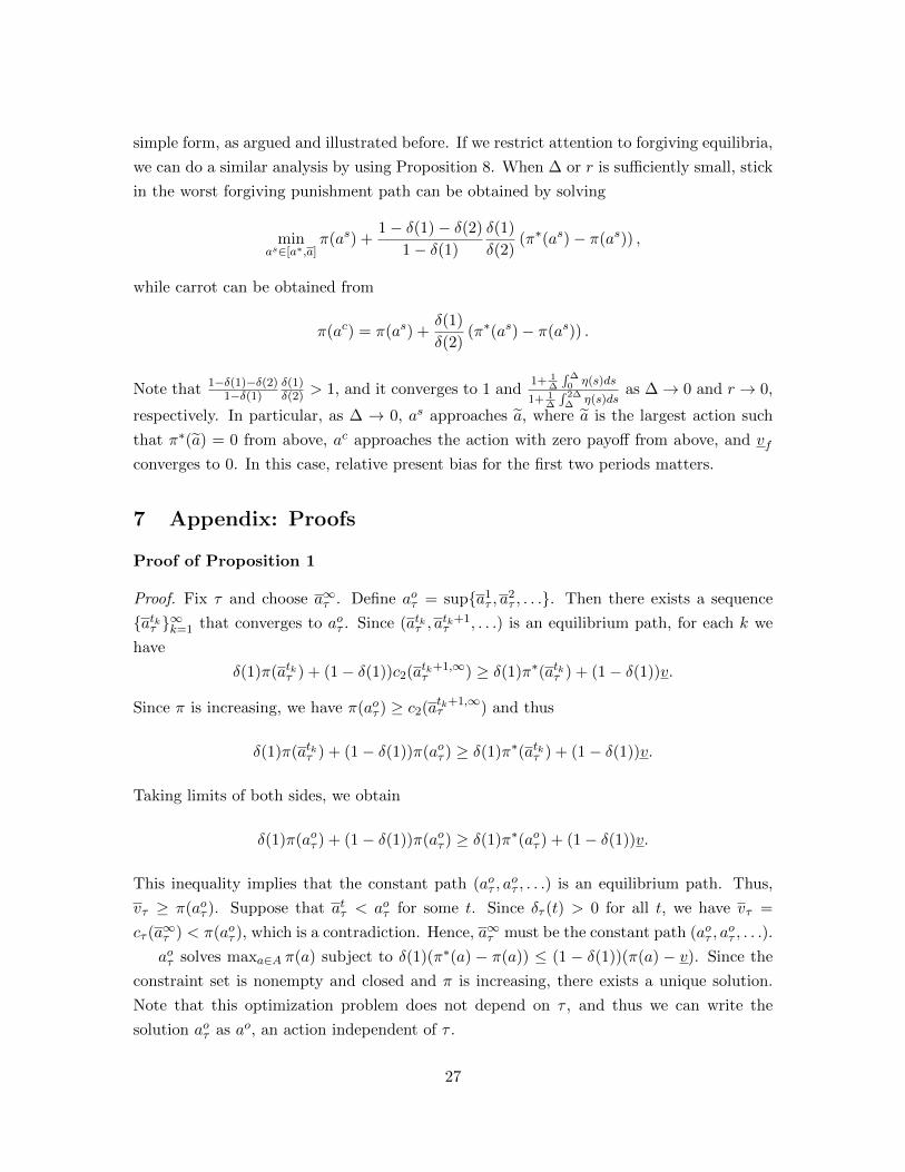
Typical graphs of the functions π(a) and π∗(a) are illustrated in Figure 1. Differen-

tiability is assumed just for the sake of exposition. Most of our results do not depend on

differentiability. Since π is increasing, π(a∗) is the unique action that achieves the maximum

symmetric payoff. We will use π = π(a∗) and π = π(0) to denote the maximum and the

minimum stage game payoffs, respectively. Since π∗ is nondecreasing and the symmetric

minmax payoff is 0, π∗(0) = 0. Note that π = π(0) < π∗(0) = 0 as 0 is not a Nash equi-

librium. The last part of the assumption means that the gain from a unilateral deviation

becomes larger (or unchanged) as the action profile moves away from the unique symmetric

Nash equilibrium.

All these assumptions are standard and satisfied in many applications. We show that a

Cournot competition game with capacity constraint satisfies the above assumptions.

Example: Cournot Game

Consider a Cournot game where the inverse demand function is given by p(Q) =

max{A − BQ, 0} for some A,B > 0, where Q =∑n

i=1 qi. Each firm’s marginal cost is

constant c ∈ (0, A). Assume that each firm can produce up to the capacity constraint q.5

We assume that q is large enough to satisfy A−Bnq − c < 0. Then π and π∗ are given as

4We use increasing/decreasing and nondecreasing/nonincreasing to distinguish strict monotonicity andweak one.

5The existence of such a bound on the production set can be assumed without loss of generality in thestandard case (Abreu [1]). However this is a substantial assumption in our setting as the equilibrium notionwe use is not even the standard Nash equilibrium. See footnote 9.

5

a

π

0 a∗

π

π

π∗(a)

π(a)

πNE

aNE

1

Figure 1: Graphs of π(a) and π∗(a).

follows.

π(q) = (max{A−Bnq, 0} − c) q,

π∗(q) =1

B

(max

{A−B(n− 1)q − c

2, 0

})2

.

Let q∗ = A−c2Bn be the production level that maximizes the joint profit. For each q ∈ (0, q∗),

there exists q ∈ (q∗, q) such that π(q) = π(q) and π∗(q) < π∗(q). This means that we can

replace q with q in any equilibrium. So it is without loss of generality to restrict attention

to the production set [q∗, q]. Identify q with 0 and q∗ with a∗. Then π and π∗ satisfies all

the assumptions except for the last one about π∗(a)− π(a). This assumption is satisfied if

(n+ 1)c > n−1n A (then π∗(q)− π(q) is increasing for q > qNE).

2.2 Present Bias and Future Bias

As already mentioned, when a player evaluates a path a∞ ∈ A∞ that begins in period τ in

the beginning of the game, he uses discount factors (δ(τ), δ(τ + 1), . . .). We can normalize

them so that their sum is equal to 1. For τ = 1, 2, . . . and t = 1, 2, . . ., we define

δτ (t) =δ(t+ τ − 1)

1−∑τ−1

k=1 δ(k).

6

Let cτ (a∞) =∑∞

t=1 δτ (t)π(at) for τ = 1, 2, . . .. cτ is the payoff function that is used to

evaluate paths starting in period τ in the beginning of the game. Note that δ1(t) = δ(t) for

all t and thus c1(a∞) = V (a∞), where V (a∞) = V (π(a1), π(a2), . . .) denotes the value of

the path a∞ ∈ A∞.

We say that a player may exhibit “present bias” or “future bias” when {δτ (t)} and

{δτ ′(t)} are systematically different unlike the standard case with geometric discounting.

Since discount factors sum up to 1, they can be regarded as probability distributions. So

we use the language of stochastic ordering to define a variety of biases.

Definition 1 (Present Bias and Future Bias via MLRP).

1. (Present Bias via MLRP): {δ′(t)}∞t=1 ∈ Γ is more present biased relative to

{δ′′(t)}∞t=1 ∈ Γ in the MLRP (monotone likelihood ratio property) sense if δ′(t1)δ′(t2) ≥

δ′′(t1)δ′′(t2) for all t1 and t2 such that t1 < t2. {δ(t)}∞t=1 ∈ Γ exhibits present bias in the

MLRP sense if {δτ (t)}∞t=1 ∈ Γ is more present biased relative to {δτ ′(t)}∞t=1 ∈ Γ in the

MLRP sense for any τ and τ ′ such that τ < τ ′.

2. (Future Bias via MLRP): {δ′(t)}∞t=1 ∈ Γ is more future biased relative to {δ′′(t)}∞t=1 ∈Γ in the MLRP sense if δ′(t2)

δ′(t1) ≥δ′′(t2)δ′′(t1) for all t1 and t2 such that t1 < t2. {δ(t)}∞t=1 ∈ Γ

exhibits future bias in the MLRP sense if {δτ (t)}∞t=1 ∈ Γ is more future biased relative

to {δτ ′(t)}∞t=1 ∈ Γ in the MLRP sense for any τ and τ ′ such that τ < τ ′.

To see that this definition is consistent with the standard notion of biases, consider the

following example. When comparing period 2 payoff π2 and period 3 payoff π3, “period

2-self” puts relatively more weight on π2 than period 1-self if a player is present biased.

This means that δ(1)δ(2) ≥

δ(2)δ(3) . This is equivalent to δ(1)

δ(2) ≥δ2(1)δ2(2) , which corresponds to the

case of τ = 1, τ ′ = 2, t1 = 1, t2 = 2 in the above definition of present bias.6

The next definition of biases is based on the notion of first-order stochastic dominance.

Definition 2 (Present Bias and Future Bias via FOSD).

1. (Present Bias via FOSD): {δ′(t)}∞t=1 ∈ Γ is more present biased relative to {δ′′(t)}∞t=1 ∈Γ in the FOSD sense if

∑kt=1 δ

′(t) ≥∑k

t=1 δ′′(t) for all k = 1, 2, . . .. {δ(t)}∞t=1 ∈ Γ ex-

hibits present bias in the FOSD sense if {δτ (t)}∞t=1 ∈ Γ is more present biased relative

to {δτ ′(t)}∞t=1 ∈ Γ in the FOSD sense for any τ and τ ′ such that τ < τ ′.

2. (Future Bias via FOSD): {δ′(t)}∞t=1 ∈ Γ is more future biased relative to {δ′′(t)}∞t=1 ∈Γ in the FOSD sense if

∑kt=1 δ

′′(t) ≥∑k

t=1 δ′(t) for all k = 1, 2, . . ..{δ(t)}∞t=1 ∈ Γ ex-

6If {δ(t)}∞t=1 is more present biased than {δk(t)}∞t=1 in the MLRP sense for any k, then {δτ (t)}∞t=1 is morepresent biased than {δτ+k(t)}∞t=1 in the MLRP sense for any τ and any k. Hence it suffices to set τ = 1 inDefinition 1.

7

hibits future bias in the FOSD sense if {δτ (t)}∞t=1 ∈ Γ is more future biased relative

to {δτ ′(t)}∞t=1 ∈ Γ in the FOSD sense for any τ and τ ′ such that τ < τ ′.

This notion of present bias captures the effect that the tendency to put relatively more

weight on period t payoff against the continuation payoff from period t + 1 diminishes as

t increases. Clearly, if a player is present biased (resp. future biased) in the MLRP sense,

then the player is present biased (resp. future biased) in the FOSD sense.

Note that all these biases are defined with weak inequalities. Hence any of these bi-

ased preferences include the standard geometric discounting as a special case. A player

exhibits strict present/future bias in the MLRP/FOSD sense if all the inequalities in the

corresponding definition hold strictly. For example, {δ′(t)}∞t=1 ∈ Γ is strictly more present

biased relative to {δ′′(t)}∞t=1 ∈ Γ in the MLRP sense, if δ′(t1)δ′(t2) >

δ′′(t1)δ′′(t2) for all t1 and t2 such

that t1 < t2.

We often use following class of discounting with δ ∈ (0, 1) and βt > 0, t = 0, 1, . . ., which

is not normalized:

V (a∞) = β0π(a1) + β1δπ(a2) + β2δ2π(a3) + β3δ

3π(a4) + · · · .

We assume that β0 = 1 without loss of generality. We also assume that βt, t = 1, 2, . . ., is

bounded above, which implies that the weighted sum of stage game payoffs is finite given

any δ ∈ (0, 1). When βt, t = 0, 1, . . ., satisfies these assumptions, we call this discounting

{βt}t-weighted discounting. This is a useful class of discounting as it nests many familiar

discountings. It reduces to the standard geometric discounting if βt = 1 for all t. It

corresponds to the standard quasi-hyperbolic (β–δ) discounting (with present bias) if β1 =

β2 = β3 = · · · = β for some β ∈ (0, 1). We can also represent a genuine hyperbolic

discounting by choosing appropriate βt, t = 1, 2, . . .. It is straightforward to show that

{βt}t-weighted discounting exhibits strict present bias (resp. future bias) in the MLRP

sense if and only if βt+1

βtis increasing (resp. decreasing) with respect to t, in which case the

ratio converges in [0, 1] as t goes to infinity.

2.3 Agent Subgame Perfect Equilibrium

In standard subgame perfect equilibrium, each player can use any possible continuation

strategy at any history as a deviation. Without time consistency, however, it is not obvious

which type of deviations a player would think possible, since it may be the case that some

deviation is profitable from the viewpoint of the current self, but not from the viewpoint of

future selves.

In this paper, we assume that each player believes that future selves (as well as all the

other players) would stick to the equilibrium strategy if he deviates in the current period.

8

One interpretation of this assumption is that a player is a collection of agents who share the

same preference and act only once. This type of equilibrium notion is standard and used in

numerous papers such as Phelps and Pollak [11] and Peleg and Yaari [10]. We adapt this

notion of equilibrium and call it Agent Subgame Perfect Equilibrium (ASPE). The formal

definition is as follows.

Definition 3 (Agent Subgame Perfect Equilibrium). A strategy profile s ∈ S is an agent

subgame perfect equilibrium (ASPE) if

Vi(a(s|ht)) ≥ Vi((a′i, a1−i(s−i|ht)), a(s|ht,(a′i,a1

−i(s−i|ht ))))

for any a′i ∈ A, any ht ∈ H and any i ∈ N .

To understand this definition, compare it to the standard definition of subgame perfect

equilibrium.

Definition 4 (Subgame Perfect Equilibrium). A strategy profile s ∈ S is a subgame perfect

equilibrium (SPE) if

Vi(a(s|ht)) ≥ Vi(a(s′i, s−i|ht))

for any s′i ∈ S, any ht ∈ H and any i ∈ N .

All possible deviations are considered for SPE, whereas only one-shot deviations are

considered for ASPE. With the standard geometric discounting, the one-shot deviation

principle applies: if there is no profitable one-shot deviation, then there is no profitable

deviation. Hence there is no gap between ASPE and SPE. With general discounting, the

one-shot deviation principle would fail because of time inconsistency. Therefore the set of

SPE is in general a strict subset of ASPE.7,8,9

Agent subgame perfect equilibrium s∗ is strongly symmetric if every player plays the

same action at any history, i.e. s∗i (ht) = s∗j (ht) for any ht ∈ H and any i, j ∈ N . There

7In general, the set of equilibria would shrink as more deviations are allowed. However ASPE remainsunchanged even if we allow for a larger class of finite period deviations where every deviating-self along adeviation path is required to gain strictly more than what he would have obtained by playing according tothe continuation equilibrium. See Obara and Park [8].

8Chade, Prokopovych and Smith [3] shows that the sets of equilibrium payoffs for these two notions ofequilibrium coincide for β–δ discounting.

9Unbounded stage game payoffs, which we exclude by assumption, would be another source of gap betweenSPE and ASPE. For example, we would have many “crazy” ASPE even with geometric discounting if thereis no capacity constraint (hence the symmetric payoff π is unbounded below) in the Cournot game. Inparticular, we can construct the following type of ASPE with an arbitrary low payoff: every firm producessome large q′ and makes negative profits because otherwise every firm would produce even larger amountq′′ � q′ in the next period and so on. Such behavior cannot be sustained in SPE, or even in Nash equilibriumif q′ is too large, but can be sustained in ASPE. So the existence of capacity constraint q is a substantialassumption that excludes this type of ASPE.

9

exists at least one strongly symmetric agent subgame perfect equilibrium in (G, {δ(t)}∞t=1)

for any {δ(t)}∞t=1 because we assume that there exists a symmetric Nash equilibrium for G

and playing this symmetric equilibrium at any history is an ASPE.

Let AASPE ⊆ A∞ be the set of (strongly symmetric) agent subgame perfect equilibrium

paths. Since the time preference is invariant, the set of ASPE continuation paths from any

period is also AASPE . We define vτ = supa∞∈AASPE cτ (a∞) and vτ = infa∞∈AASPE cτ (a∞)

for τ = 1, 2, . . .. Obara and Park [8] shows that vτ and vτ can be exactly attained (i.e. sup

and inf can be replaced by max and min) for any τ in more general settings. We denote any

equilibrium path to achieve vτ and vτ by a∞τ and a∞τ respectively. Of particular interest

among these values is v2, which is the the worst equilibrium continuation payoff from period

2, since it determines the size of maximum punishment. We will simply denote it by v and

call it the worst punishment payoff. We also call a∞2 a worst punishment path and simply

denote it by a∞. As in the usual case, we can always use v as the punishment payoff without

loss of generality when we check incentive constraints.

3 Best Equilibrium

In the standard case, the best (strongly symmetric) equilibrium payoff is always achieved

by a constant path. We first observe that this result holds even with general discounting.

The following proposition shows that the best equilibrium path a∞τ to achieve vτ is given

by the unique constant path independent of τ .

Proposition 1. For all τ = 1, 2, . . ., a best equilibrium (continuation) path a∞τ is unique

and given by a constant path (ao, ao, . . .) where ao ∈ (aNE , a∗] is independent of τ . Moreover,

ao = a∗ when δ(1) is small enough.

The proof of this proposition is standard. Let ao be the most efficient symmetric action

profile that can be achieved in any equilibrium. Then the constant path (ao, ao, . . .) must

be an equilibrium path (hence the best equilibrium path) as well. The incentive constraint

to play ao is satisfied because the value of this path is at least as high as the value of any

equilibrium path where ao is played in the initial period and we can always use the same

worst punishment path.

This proposition also says that the best equilibrium payoff is strictly higher than the

stage game Nash equilibrium payoff. This follows from differentiability of π and π∗. The

one-shot deviation constraint for any constant path (a, a, . . . ) is given by

δ(1) (π∗(a)− π(a)) ≤ (1− δ(1)) (π(a)− v) .

Note that a = aNE satisfies the above constraint and (π∗)′(aNE)− π′(aNE) = 0; hence the

10

deviation gain on the left-hand side is roughly 0 around aNE as there is no first-order effect.

On the other hand, the continuation payoff loss on the right-hand side increases strictly at

aNE . Hence this constraint is slack for a that is slightly above aNE . For any a > aNE ,

the above incentive constraint is satisfied for sufficiently small δ(1), because v ≤ π(aNE).

Hence we can achieve the most efficient action a∗ and payoff π at ASPE when δ(1) is small

enough.

Since vτ = π(ao) for all τ , we will denote this common value by v. To compute v, we

need to know how harsh a punishment can be in ASPE. In the following sections, we study

the structure of worst punishment paths and characterize the set of all equilibrium payoffs

under various assumptions.

4 Characterization of Equilibrium: Future Bias

The structure of worst punishment paths and the set of equilibrium payoffs depend on the

structure of intertemporal bias. It turns out that the case of future bias is simpler and more

tractable. Thus we first examine the case of future bias.

As a preliminary, we prove the following property of the worst punishment path that

holds in general, not just for future bias.

Proposition 2. For all τ = 1, 2, . . ., vτ < π(aNE) and a1τ ≤ aNE for any worst punishment

path a∞τ .

The first part of the proposition follows from differentiability of the payoff functions

as was the case with Proposition 1. In particular, we can show that (a′, aNE , aNE , . . .)

can be an equilibrium for some a′ < aNE that is close to aNE . The second part follows

from the observation that any action a ∈ (aNE , a∗] in the initial period can be replaced

by aNE without affecting any incentive constraints. Thus every worst punishment path

starts with an action that is no more efficient than aNE . But how does the path look like

from the second period? Call any path (as, ac, ac, . . .) such that as < ac a stick-and-carrot

path. Abreu [1] shows that, with geometric discounting, the worst punishment payoff v

can be achieved by a stick-and-carrot punishment path with ac = ao, where one-period

punishment is immediately followed by the best equilibrium path (ao, ao, . . .). Furthermore

it is the unique worst punishment path when π∗ is increasing to the right of as.

We show that the worst punishment payoff can be achieved by a version of stick-and-

carrot path where the play would eventually go back to the best equilibrium path when

the players exhibit future bias in the MLRP sense. We also provide two conditions under

which the worst punishment path is unique. The first condition is essentially the same as

the above condition on the slope of π∗. The second condition, which is new, is that the

11

future bias is strict in some sense. The bottom line is that the structure of stick-and-carrot

punishment is robust with respect to future bias.

Proposition 3. Suppose that {δ(t)}∞t=1 exhibits future bias in the MLRP sense. Then the

following hold:

1. There exists a worst punishment path a∞ that takes the following form:

a∞ = (0, . . . , 0︸ ︷︷ ︸K times

, a, ao, ao, . . .), where 0 appears K times for some finite K ≥ 0 and

a ∈ [0, ao). A worst punishment path in the above form is unique (i.e. K and a

are uniquely determined), and the incentive constraint to play a1 on the path a∞ is

binding, that is,

δ(1)(π∗(a)− π(a)) = δ(2)(π(ao)− π(a)) when K = 0, and

δ(1)(−π) = δ(K + 1)(π(a)− π) + δ(K + 2)(π(ao)− π(a)) when K ≥ 1.

2. The above path is the unique worst punishment path if (i) K = 0 and π∗ is increasing

to the right of a1 or (ii) {δ(t)}∞t=1 is strictly more future biased relative to {δ2(t)}∞t=1

in the MLRP sense.

The worst punishment path may require multiple periods of “stick” to generate a harsh

enough punishment. This is due to the assumption that the stage game payoff is bounded.

Otherwise this path would be a usual stick-and-carrot path with one period of stick. For

the standard geometric discounting, which satisfies the assumption for the proposition,

there are many other worst punishment paths. For example, a simple stick-and-carrot path

(0, a′, a′, . . .) would be another worst punishment paths, where a′ satisfies V (0, a′, a′, . . .) =

V (0, . . . , 0, a, ao, ao, . . .). The second part of the proposition shows that such multiplicity of

punishment paths is eliminated by strict future bias. This is because backloading payoffs

does make a punishment strictly more harsh in this case.

The idea of the proof is simple. We can replace any worst punishment path a∞ with the

(unique) path that takes the above form and has an equal initial value. The only binding

incentive constraint is the one in the first period. Since the first period action of this new

path is no more than the first period action of the original path and π∗ is nondecreasing,

this new path is indeed an ASPE path. By construction, V (0, . . . , 0, a, ao, ao, . . .) = V (a∞).

Then the assumption of future bias implies c2(0, . . . , 0, a, ao, ao, . . .) ≤ c2(a∞)(= v). Hence

this new ASPE path achieves the worst punishment value v from the viewpoint of “period-0”

player, against whom this punishment would be used upon his deviation.

If a player is strictly more future biased than his period-2 self and a∞ does not take

this version of stick-and-carrot form, then we would have c2(0, . . . , 0, a, ao, ao, . . .) < v at

12

the end of the above argument, which is a contradiction. Hence the worst punishment path

must take this particular form in this case and clearly there exists the unique such path to

generate v.

The assumption of strict future bias in the MLRP sense is not weak. But suppose that

K = 0 and the worst punishment payoff can be achieved by a standard stick-and-carrot

path (this is the case, for example, if the capacity constraint is large enough in the Cournot

game). Then what we would need for the uniqueness result is just that δ(t2)δ(1) >

δ2(t2)δ2(1) for all

t2 > 1 (i.e. t1 = 1 is enough). For example this condition is satisfied for β–δ discounting

with β > 1, although {δ(t)}∞t=1 is not strictly more future biased relative to {δ2(t)}∞t=1 in

this case.

Once we characterize the structure of worst punishment paths, we can derive the set of

equilibrium payoffs. For the case of future bias, the worst equilibrium path coincides with

the worst punishment path characterized above. This is because the same argument as

above implies that the worst equilibrium path can take exactly the same form as the worst

punishment path, thus the worst equilibrium payoff is given by V (a∞). This is a trivial

fact with geometric discounting, but does not hold in general with general discounting. The

following proposition also proves the convexity of the equilibrium payoff set.

Proposition 4. Suppose that {δ(t)}∞t=1 exhibits future bias in the MLRP sense. Let a∞

be the worst punishment path in the form described in Proposition 3. Then the set of

equilibrium payoffs is given by the closed interval [v1, v], where v1 = V (a∞).

We can show that any payoff between v1 and v can be supported by a similar, but more

generous stick and carrot (with K ′ ≤ K). We do not use a public randomization device to

convexify the equilibrium payoff set.

Based on Proposition 3, we can compute the value of the worst punishment payoff for

{βt}t-weighted discounting that is future biased in the MLRP sense and more future biased

than the geometric discounting. For this class of discounting, which includes the geometric

discounting as a special case, we can also show that the worst punishment payoff in the

limit (as δ → 1) is strictly smaller than the stage game minmax payoff 0 if and only if the

discounting is not geometric.

Proposition 5. Suppose that the time preference is given by {βt}t-weighted discounting. If

{βt}t-weighted discounting exhibits future bias and is more future biased than the geometric

discounting with the same δ both in the MLRP sense, then the following hold:

1. βt is nondecreasing with respect to t and converging to limt→∞ βt <∞.

2. Let a∞ = (0, . . . , 0︸ ︷︷ ︸K times

, a, ao, ao, . . .) be the worst punishment path in the form described in

Proposition 3, where K ≥ 0 and a ∈ [0, ao). The worst punishment payoff v is given

13

by the following value:

π(ao)− π∗(a)− π(a)∑∞t=1 βtδ

t

when K = 0, and

δ

(1− δ)(∑∞

t=1 βtδt)

{K−1∑t=0

[(βt+1 − βt) δt

]π + (βK+1 − βK) δKπ(a)

+

∞∑t=K+1

[(βt+1 − βt) δt

]π(ao)

}

when K ≥ 1. K is nondecreasing as δ increases and goes to ∞ as δ → 1.

3. As δ → 1, v and v1 converge to the same limit

limt βt − 1

limt βtπ,

which is strictly smaller than the symmetric minmax payoff 0 if and only if the {βt}t-weighted discounting is not the geometric discounting.

A few remarks are in order. First, the third result follows from the fact that limt βt > 1

if and only if the discounting is not geometric. To see this, note that the two MLRP

assumptions imply βtβt−1

≥ βt+1

βtand βt ≥ 1 for all t = 1, 2, . . . respectively. This implies

that βt must be nondecreasing with diminishing increasing rates. Hence limt βt = 1 if and

only if βt = 1 for all t ≥ 1 (remember that β0 = 1) if and only if the discounting is the

geometric discounting (because βt is bounded above). Otherwise limt βt > 1. Second, more

importantly, an actual impact of bias on the equilibrium payoff can be huge. Note that all

these results are stated in terms of normalized payoffs. In terms of total payoffs, both the

worst punishment payoff and the worst equilibrium payoff diverge to negative infinity as δ

goes to 1 whenever the discounting is not geometric in this class.

We should be careful about how to interpret large δ here. There are usually two ways

to interpret this parameter. One interpretation is that players are more patient. The other

interpretation is that players are playing the game more frequently. The first interpreta-

tion is more appropriate here because the bias structure is fixed. One advantage of our

framework is that we can also model the second effect formally. In Section 6, we examine

the limit equilibrium payoff when the length of periods becomes shorter while keeping the

intertemporal bias structure unchanged with respect to actual time.

14

5 Characterization of Equilibrium: Present Bias

Next we examine the structure of equilibrium paths and the set of equilibrium payoffs for

the case of present bias. This is possibly a more interesting case, but more complicated.

In this section, we introduce the following additional assumptions on the stage game to

facilitate our analysis.

Assumption 2. π is strictly concave and π∗ is convex.

One implication of this assumption is that the set of a for which the constant play of a is

an ASPE path is a closed interval [a, ao], where a is the unique action below aNE such that

the incentive constraint is binding, i.e. δ(1) (π∗(a)− π(a)) = (1 − δ(1)) (π(a)− v). This

follows from Assumption 2 because π(a)− δ(1)π∗(a) is strictly concave.

We first focus on an interesting, but restricted class of equilibrium. Then we move on

to a fully general case.

5.1 Forgiving Punishment and Forgiving Equilibrium

It makes sense to punish a deviator as soon as possible in order to make the punishment

as effective as possible. The stick-and-carrot strategy takes this idea to the extreme: it

punishes a deviator as much as possible immediately after his deviation, then forgives him

afterward, i.e. goes back to the original cooperative path. In another word, any necessary

punishment is as front loaded as possible.

We consider a particular class of punishment scheme: forgiving punishment, which is

based on this idea, but more general than a simple stick-and-carrot scheme. It imposes the

harshest punishment in the first period and then imposes less and less severe punishments

over time. So a deviator is gradually forgiven along a forgiving punishment path. Formally,

let A∞f = {a∞ ∈ A∞ : a1 ≤ a2 ≤ · · · } be the set of paths where payoffs are nondecreasing

over time. We say that a path is forgiving if it belongs to this set. In this subsection,

we restrict attention to strongly symmetric equilibria that prescribe a path in A∞f after

every history. We call such equilibria forgiving equilibria. With geometric discounting, it

is without loss of generality to focus on forgiving equilibria: every equilibrium payoff can

be generated by a forgiving equilibrium. Let AASPEf be the set of all forgiving equilibrium

paths.

It is easy to show as in Proposition 1 that the best forgiving equilibrium path is given by

a constant path, which is denoted by (aof , aof , . . .). We define the worst forgiving punishment

payoff by vf = infa∞∈AASPEfc2(a∞). Since (aNE , aNE , . . .) ∈ AASPEf , AASPEf is nonempty.

Since A∞f is compact, we can show the existence of a forgiving equilibrium path that achieves

vf as usual. We denote a worst forgiving punishment path by a∞f .

15

The following proposition characterizes the worst forgiving punishment path when the

time preference exhibits (strict) present bias in the FOSD sense.

Proposition 6. Suppose that {δ2(t)}∞t=1 is more present biased relative to {δ3(t)}∞t=1 in the

FOSD sense.10 Then the following holds:

1. There exists a worst forgiving punishment path that takes the following simple stick-

and-carrot form: a∞f = (as, ac, ac, . . .) where as < ac. Moreover, as is never the worst

action 0 if δ(1) > δ2(1) and π∗′(0) is small enough.

2. The above path is the unique worst forgiving punishment path if {δ2(t)}∞t=1 is strictly

more present biased relative to {δ3(t)}∞t=1 in the FOSD sense.

Take any forgiving punishment path a∞. Then we can find some a′ to satisfy V (a∞) =

V (a1, a′, a′, . . .) and easily verify that (a1, a′, a′, . . .) is another ASPE path. The present bias

implies that (a1, a′, a′, . . .) is at least as a harsh punishment as a∞ (i.e. c2(a1, a′, a′, . . .) ≤c2(a∞)). Thus it is without loss of generality to focus on punishments of the form (as, ac, ac, . . .)

for forgiving equilibria. This observation is valid with geometric discounting and not new.

However the way in which (as, ac) is determined is very different from the standard

case. With geometric discounting, the incentive constraint can be relaxed by making stick

worse and carrot better while keeping the discounted average payoff constant, since π∗(as)

decreases as as decreases. Hence the gap between stick and carrot is maximized, and

therefore either 0 is used as stick or ao is used as a carrot. With present bias, we also see

the opposite force at work, which tends to reduce the gap between stick and carrot. If we

increase as and decrease ac in such a way that V (as, ac, ac, . . .) does not change, then this

path generates a more harsh punishment if it is still an ASPE. Intuitively, due to present

bias, we can decrease ac by relatively a large amount by increasing as only slightly. From a

deviator’s viewpoint in one period before, ac decreases too much thus c2 goes down. This

effect pushes as up and pushes ac down. The incentive cost associated with this perturbation

depends on how quickly π∗(as) increases as as increases. Thus, as claimed in the latter part

of Proposition 6-1, if the slope of π∗ is small at 0, then this incentive cost is relatively small

hence as must be strictly positive.

To be more explicit, the pair of stick and carrot (as, ac) that constitutes a worst forgiving

10This is equivalent to δ2(1) ≥ δτ (1) for all τ ≥ 3.

16

punishment path can be obtained by solving the following minimization problem:

minas,ac∈A

δ2(1)π(as) + (1− δ2(1))π(ac)

s.t.δ(1)

1− δ(1)(π∗(as)− π(as)) ≤ δ2(1)(π(ac)− π(as)),

δ(1)

1− δ(1)(π∗(ac)− π(ac)) ≤ δ2(1)(π(ac)− π(as)).

The first constraint corresponds to the one-shot deviation constraint for as and the second

constraint corresponds to the one-shot deviation constraint for ac. When δ(1) is small,

we can drop the second constraint because the obtained solution as and ac automatically

satisfies as < ac < aof .

In the following proposition, we show that the worst forgiving equilibrium payoff can also

be achieved by a (different) stick and carrot path and that the set of forgiving equilibrium

payoffs is convex.

Proposition 7. Suppose that {δ2(t)}∞t=1 is more present biased relative to {δ3(t)}∞t=1 in the

FOSD sense. Then the following hold:

1. There exists a worst forgiving equilibrium path that takes the following form: a∞1,f =

(as, ac, ac, . . .) where as ≤ ac. If δ(1) ≥ δ2(1), then as ≤ as < ac ≤ ac for any worst

forgiving punishment path a∞f = (as, ac, ac, . . .) in the stick-and-carrot form.11

2. The set of forgiving equilibrium payoffs is given by a closed interval[v1,f , v1,f

], where

v1,f = V (a∞1,f ) and v1,f = π(aof ).

3. All the three payoffs vf , v1,f , v1,f and the associated equilibrium paths are com-

pletely determined by δ(1) and δ2(1) only. vf (δ(1), δ2(1)) decreases as δ(1) decreases

(while keeping δ2(1) constant) or as δ2(1) increases (while keeping δ(1) constant).

v1,f (δ(1), δ2(1)) decreases as δ2(1) increases. v1,f (δ(1), δ2(1)) increases up to π as

δ(1) decreases or as δ2(1) increases.

Propositions 7-3 implies that it is without loss of generality to use the standard β–

δ discounting provided that the above assumption of present bias is satisfied. In another

word, we cannot identify βt, t ≥ 2 from equilibrium behavior as long as we focus on forgiving

equilibria (even if we can learn what the players would have played off the equilibrium path).

For β–δ discounting, δ(1) = 1−δ1−δ+βδ and δ2(1) = 1 − δ. So, for any pair of (δ(1), δ2(1)) ∈

(0, 1)2, we can find appropriate β > 0 and δ ∈ (0, 1) to generate them, namely β =1−δ(1)δ(1)

δ2(1)1−δ2(1) and δ = 1− δ2(1). In particular, we have β ≤ 1 when δ(1) ≥ δ2(1).

11If δ(1) ≤ δ2(1), then as ≥ as and ac ≤ ac.

17

Proposition 1 of Chade, Prokopovych and Smith [3] shows that the set of equilibrium

payoffs expands weakly as β increases and δ decreases while δ(1) is fixed. Our result is con-

sistent with this proposition as such change of parameters induces δ2(1) to increase. Chade,

Prokopovych and Smith [3] also shows that the set of equilibrium payoffs is nonmonotonic

in either β or δ. Our result is consistent with this non-monotonicity result as well. As β

increases, δ(1) becomes smaller while δ2(1) is unaffected, and the effect of δ(1) on v1,f is

ambiguous. As δ increases, δ(1) and δ2(1) both decrease. Again their effects on v1,f and

v1,f are ambiguous.

As before, we can characterize the worst forgiving punishment payoff given {βt}t-weighted discounting when δ approaches 1.

Let as∗ be a solution of the following minimization problem:

mina∈A

π(a) + C({βt}t) (π∗(a)− π(a)) ,

where C({βt}t) =1− β1∑∞

t=1 βt

β1. Define ac∗ by the following equation:

π(ac∗) = π(as∗) +1

β1(π∗(as∗)− π(as∗)) . (1)

Proposition 8. Suppose that the time preference is given by {βt}t-weighted discounting

that exhibits present bias in the MLRP sense and is not the geometric discounting. Then

the following hold:

1. as∗ and ac∗ are uniquely determined, and π(as∗)+C({βt}t) (π∗(as∗)− π(as∗)) > 0 and

π(ac∗) > 0.

2. The worst forgiving punishment path that is obtained in Proposition 6 converges to

(as∗, ac∗, ac∗, . . .) as δ → 1.

3. vf converges to π(as∗) + C({βt}t) (π∗(as∗)− π(as∗)) as δ → 1. If∑∞

t=1 βt =∞, then

the limit coincides with π(ac∗).

When δ is large, δ(1) is small. Hence we only need to consider the one-shot deviation

constraint for as, which can be written as π(ac) ≥ π(as) + 1β1δ

(π∗(as)− π(as)). This

constraint must be binding. Hence we can use this to eliminate ac from the objective

function. As δ → 1, the objective function to be minimized (to find as) converges to the

objective function for the minimization problem for as∗. Then the limit of the solutions for

the minimization problems as δ → 1 converges to the solution of the limit minimization

problem, which is as∗. ac∗ is obtained by computing the limit of the binding constraint (1).

18

Proposition 8 implies the the worst punishment payoff for the class of forgiving equilibria

is strictly positive (hence above the the minmax payoff 0) for any present-biased discounting

that is not geometric discounting. The {βt}t-weighted discounting is present biased if and

only if βtβt−1

≤ βt+1

βtfor all t. It coincides with geometric discounting (with discount factor

βδ) if and only if βt+1

βtis some constant β ∈ (0, 1], since {βt} must be bounded above by

assumption. Then {βt}t-weighted discounting is not geometric discounting if and only if

one of the above inequalities hold strictly. In this case, it can be shown that C({βt}t) > 1,

which implies that vf > 0 even as δ goes to 1.12

This does not mean that the true worst punishment payoff is strictly positive because

v is in general smaller than vf as we will see. However we will show that v = vf > 0 holds

for β–δ discounting with β ∈ (0, 1), which is present biased.

5.2 General Case

Next we characterize the set of ASPE without any restriction. A question of interest is

whether restricting attention to forgiving punishments is without loss of generality (i.e.

vf = v) or not. The following proposition partially characterizes the structure of the worst

punishment path with present bias and shows that a forgiving punishment path is never a

worst punishment path.

Proposition 9. Suppose that {δ(t)}∞t=1 exhibits present bias in the FOSD sense and that

δt(1) is decreasing in t. Suppose also that δ(1) is small enough. Let a∞ be any worst

punishment path. If at,∞ is a forgiving path for some t, then at,∞ must be the worst constant

ASPE path (a, a, . . .) and t must be at least 3.

The assumption about {δ(t)}∞t=1 is weaker than assuming that {δ(t)}∞t=1 exhibits strict

present bias in the FOSD sense, since it would imply that δt(1) is decreasing in t (and

more).

This proposition suggests that a worst punishment path may exhibit a cyclical pattern.

Later in this subsection, we show an example with present bias where the unique worst

punishment path must fluctuate forever generically, although δt(1) is only weakly decreasing

and (strictly) decreasing only for t = 1, 2, 3.

Next we develop a recursive method to characterize and derive worst punishment paths.

For this purpose, we restrict our attention to {βt}t-weighted discounting where bias disap-

pears after T periods (i.e. βT = βT+k for all k = 1, 2, . . .). We assume that T ≥ 2 and treat

the case of T = 1 (i.e. β–δ discounting) separately in the next subsection. Since we have

geometric discounting from period T + 1 on, we have cT+1 = cT+2 = · · · and represent this

12For non-geometric discounting, β1 must be less than 1. If∑∞t=1 βt = ∞, then C({βt}t) = 1

β1> 1. If∑∞

t=1 βt <∞, we can show that 1− β1∑∞t=1 βt

> β1, hence C({βt}t) > 1 still holds.

19

common function by c, which is given by c(a∞) = (1− δ)[π(a1) + δπ(a2) + δ2π(a3) + · · · ].Thus the time preference has a recursive component at the end, which allows us to apply

the recursive formulation in Obara and Park [8].13 We work with stage game payoffs π

instead of actions a. Let V † = [π, π] be the set of feasible payoffs in the stage game.

The central idea of Obara and Park [8] is to decompose a sequence of stage game payoffs

in the future into a nonrecursive part and a recursive part. In this particular case, we

decompose them into the stage game payoffs from the 2nd period to the T th period and the

continuation payoff from the (T + 1)th period that is evaluated by the standard geometric

discounting (which we call the continuation score). Consider all such combinations of T −1

payoffs from the 2nd period to the T th period and a continuation score from the (T + 1)th

period that can arise in equilibrium. We can represent it as a correspondence as follows:

W ∗(π1,T−1) = {c(aT,∞) : a∞ ∈ ASSASPE , π(a1,T−1) = π1,T−1},

where we use π(at,t+k) to denote (π(at), . . . , π(at+k)).

As in Obara and Park [8], we consider an operator B which maps a correspondence

W : (V †)T−1 ⇒ V † into another correspondence W ′ : (V †)T−1 ⇒ V † as follows. Given the

correspondence W , define

w = minπ1,T−1,v

δ2(1)π1 + · · ·+ δ2(T − 1)πT−1 + [1− δ2(1)− · · · − δ2(T − 1)]v

s.t. π1,T−1 ∈ [π, π]T−1, v ∈W (π1,T−1). (2)

This is the harshest punishment according to W . Then the new correspondence W ′ is

defined by

W ′(π1,T−1) ={

(1− δ)π + δv :

δ(1)π1 + · · ·+ δ(T − 1)πT−1 + δ(T )π + [1− δ(1)− · · · − δ(T )]v

≥ δ(1)πd(π1) + (1− δ(1))w, π ≤ π ≤ π, v ∈W (π2,T−1, π)}, (3)

where W ′(π1,T−1) = ∅ if there is no pair (π, v) satisfying all the constraints in (3). πd(π)

denotes π∗(a) at a such that π(a) = π. W ′ represents the set of combinations of payoffs

from the 1st period to the (T − 1)th period and a continuation score from the T th period

that can be supported when we can pick “continuation payoffs” from W . Obara and Park

[8] shows that W ∗ is the largest fixed point of the operator B and that the graph of W ∗

(i.e. {(π1,T−1, v) : π1,T−1 ∈ [π, π]T−1, v ∈ W ∗(π1,T−1)}) is nonempty and compact. It

13Obara and Park [8] provides a recursive characterization of equilibrium payoffs for a more general classof time preferences which is eventually recursive.

20

is easy to see that a∞ is an ASPE path if and only if the corresponding payoffs satisfy

vt+T−1 ∈ W ∗(πt,t+T−2) for every t = 1, 2, . . ., where vt+T−1 = c(at+T−1,∞). Hence we can

characterize all the ASPE paths once W ∗ is obtained.

In the next proposition, we show that the operator B preserves convexity.14

Proposition 10. Let W be a correspondence from (V †)T−1 to V †. If the graph of W is

nonempty and convex, then so is the graph of W ′ = B(W ).

Since convexity is preserved under the operator B and we can start from a convex set

(V †)T to obtain the graph of W ∗ in the limit, we have the following result.

Corollary 1. The graph of W ∗ is convex.

Corollary 1 has many useful implications. Since the graph of W ∗ is convex, using public

randomization does not expand the set of equilibrium payoffs. Also, the set dom(W ∗) :=

{π1,T−1 ∈ [π, π]T−1 : W ∗(π1,T−1) 6= ∅} is convex, and W ∗ can be described by two func-

tions W ∗(π1,T−1) and W∗(π1,T−1) defined on dom(W ∗) representing the lower and up-

per boundaries of W ∗ respectively, so that W ∗(π1,T−1) = [W ∗(π1,T−1),W∗(π1,T−1)] for all

π1,T−1 ∈ dom(W ∗). Since the graph of W ∗ is convex, W ∗(π1,T−1) is convex and W∗(π1,T−1)

is concave. In fact, the upper boundary W∗(π1,T−1) is constant at v, because if a∞ is an

ASPE then so is (a1,t, ao, ao, . . .) for any t. Since W ∗(π1,T−1) is convex and the graph of

W ∗ is compact, W ∗(π1,T−1) is continuous in each argument.

For the following main result in this section, we introduce a weak form of present bias to

{βt}t-weighted discounting, namely βT−1 > βT and show that the lower boundary must be

almost self-generating. This result leads to a simple algorithm to derive a worst punishment

path.

Proposition 11. Assume {βt}t-weighted discounting such that βT−1 > βT = βT+1 = · · ·for some T ≥ 2. Then the following properties hold.

1. For any v = W ∗(π1,T−1) for any π1,T−1, (π′, v′) that decomposes v (according to (3))

must satisfy either (i) v′ = W ∗(π2,T−1, π′) or (ii) π′ = π.

2. If a∞ is a worst punishment path, then (π1,T−1, vT ) solves (2) with respect to W ∗ and

vt+T−1 = W ∗(πt,t+T−2) must hold for every t = 1, 2, . . . provided that at < a∗ for

every t.

3. Take any (π1,T−1, vT ) that solves (2) with respect to W ∗. For each vt+T−1, t = 1, 2, . . .,

let (πt+T−1, vt+T ) be the pair of (π′, v′) that satisfies vt+T−1 = (1−δ)π′+δv′ and v′ ∈14Note that πd(π) is convex, since π(a) is concave and π∗(a) is convex&nondecreasing.

21

W ∗(πt+1,t+T−2, π′), where πt+T−1 is the largest among such (π′, v′). Then the corre-

sponding path a∞ is a worst punishment path, where either (i) vt+T−1 = W ∗(πt,t+T−2)

or (ii) πt+T−2 = π holds for every t = 1, 2, . . ..

The first result is the key observation. It says that every point on the lower boundary

must be decomposed with respect to the lower boundary or possibly the right edge of W ∗.

The reason is that if (π2,T−1, π′, v′) is not on the lower boundary and π′ is not π, then we

can increase π′ and decrease v′ to obtain an equilibrium starting with payoffs π1,T−1 and

a continuation score lower than v, which is a contradiction.15 If the most efficient action

cannot be supported (i.e. ao < a∗), then π′ = π cannot hold, hence the lower boundary

must be self-generating in this case. The fact that the boundary of W ∗ is self-generating

would be helpful for us to derive W ∗ analytically or numerically.

The second result follows from the first result almost immediately. The initial point to

achieve the worst punishment payoff v must be on the lower boundary. Since πt is never

π by assumption, we can apply the first result repeatedly to show that all the subsequent

points are also on the lower boundary.

Once we obtain the lower boundary W ∗, we have a simple algorithm to construct a

worst punishment path π∞ as suggested by the last result. First, we solve (2) to obtain an

initial point (π1,T−1, vT ) where vT = W ∗(π1,T−1). Next, we decompose vT into (πT , vT+1)

as follows. We take the intersection of (1− δ)π + δv = vT and v ∈W ∗(π2,T−1, π), which is

a closed interval and nonempty by definition. Then pick (π, v) where π is the largest within

this set and define it as (πT , vT+1). Since the incentive constraint in (3) is satisfied for some

(π, v) in this set, it is guaranteed to be satisfied for (πT , vT+1). Then we can continue to

decompose vT+1 and obtain an entire entire path π∞ that satisfies vt+T−1 ∈W ∗(πt,t+T−2)

for all t = 1, 2, . . . and all the one-shot deviation constraints. This path is an ASPE path,

and clearly a worst punishment path.

Note that the decomposition at each step would be usually simpler than it appears. The

above intersection of (1− δ)π+ δv = vT and v ∈W ∗(π2,T−1, π) is typically a point: it may

not be a singleton only if the lower boundary W ∗(π2,T−1, π) has a flat part that is parallel

to (1− δ)π + δv = vT .16

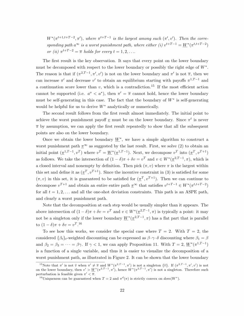
To see how this works, we consider the special case where T = 2. With T = 2, the

considered {βt}t-weighted discounting can be expressed as β–γ–δ discounting where β1 = β

and β2 = β3 = · · · = βγ. If γ < 1, we can apply Proposition 11. With T = 2, W ∗(π1,T−1)

is a function of a single variable, and thus it is easier to visualize the decomposition of a

worst punishment path, as illustrated in Figure 2. It can be shown that the lower boundary

15Note that π′ is not v when π′ 6= π and W ∗(π2,T−1, π′) is not a singleton {v}. If (π2,T−1, π′, v′) is noton the lower boundary, then v′ > W ∗(π2,T−1, π′), hence W ∗(π2,T−1, π′) is not a singleton. Therefore suchperturbation is feasible given π′ < π.

16Uniqueness can be guaranteed when T = 2 and πd(π) is strictly convex on dom(W ∗).

22

v

p

v

1 d

d

--

2

2

(1)

1 (1)

d

d-

-

1

2

34

5

6

NEp

3vv

p ¢p ¢ Sp

Figure 2: Illustration of the graph of W ∗(π).

is U-shaped with minimum attained at π(aNE) = πNE . Let (πS , πS) be the intersection of

the lower boundary v = W ∗(π) and the 45-degree line v = π, where πS = π(a) corresponds

to the payoff at the worst constant equilibrium path.

The initial payoff π1 in the worst punishment path π∞ can be obtained by solving

minπ∈[π′,π′] δ2(1)π + (1 − δ2(1))W ∗(π), and the initial point (π1,W ∗(π1)) is depicted as

point 1 in Figure 2. The subsequent payoffs π2, π3, . . . (depicted as points 2, 3, and so

on in Figure 2) cycle around πS . Starting from a payoff π1 lower than πS , the payoff in

the next period becomes higher than πS , gradually declines below πS , and then jumps

back to a payoff higher than πS , and this pattern repeats itself indefinitely. (In Figure 2,

we have π2 > π3 > π4 > πS > π5 and π6 > πS .) Thus the worst punishment path

exhibits Edgeworth cycle-type price dynamics endogenously. The continuation path πt,∞

in the worst punishment path is monotone (in particular, a forgiving path) for some t only

when we have π∞ = (π′, v, v, . . .) or we have πt,∞ decreasing initially, hit πS exactly, and

stay there forever. The latter case is a degenerate case but is shown to be possible in

Proposition 9. The former case can be eliminated if β < γ (i.e. the case of present bias in

the MRLP sense) and δ is close to 1 by Proposition 9.

Finally, observe that this recursive method can be easily applied to the opposite case

23

with βT−1 < βT = βT+1 = · · · . Proposition 10 and Corollary 1 still apply to this case.

For this case with future bias, the worst punishment path is decomposed with respect to

the upper boundary of W ∗ or possibly the left edge of W ∗. The upper boundary of W ∗ is

still a flat line at v, hence this suggests that every worst punishment path must converge

to the optimal path (ao, ao, . . .) eventually, which is consistent with our results for the case

of future bias.

5.3 β–δ Discounting

Consider quasi-hyperbolic discounting or β–δ discounting with β > 0. The next proposition

shows that, with β–δ discounting, we can focus on stick-and-carrot paths without loss of

generality when finding the worst punishment payoff.

Proposition 12. Assume β–δ discounting where β > 0 and δ ∈ (0, 1). Then there exists a

worst punishment path a∞ of the form a∞ = (as, ac, ac, . . .) where as < ac.

The idea is similar to that behind forgiving punishments. Since the time preference

becomes geometric discounting from the second period on, we can replace the path from

the second period with a constant path without affecting the values of c2 and V . Hence the

incentive to play the period-1 action a1 is preserved while the incentive constraint to play

the constant path (ac, ac, . . .) is satisfied if π(a1) ≤ π(ac), which is the case in any worst

punishment path. Thus the worst punishment payoff is achieved by a stick-and-carrot path.

This result implies that, with β–δ discounting, it is without loss of generality to focus on

forgiving punishments (i.e. v = vf ).

When β > 1, β–δ discounting exhibits future bias in the MLRP sense (but not strictly).

We know that there is a worst punishment path of the form described in Proposition 3 in

this case. By Proposition 5, the worst punishment payoff is β−1β π < 0 when δ is large.

Proposition 12 shows that there is also another worst punishment path in the stick-and-

carrot form (as, ac, ac, . . .). In particular, if the worst punishment path obtained from

Proposition 3 is not a stick-and-carrot path (which implies as = 0), then we can construct

a worst punishment (as, ac, ac, . . .), where as = 0 and ac < ao by smoothing out the payoffs

from the second period.

When β < 1, β–δ discounting exhibits present bias in the MLRP sense. Thus our results

on forgiving punishments with present bias (Propositions 6–8) are applicable to this case.

Proposition 6-1 suggests that the worst punishment path in the stick-and-carrot form may

need to use a carrot ac smaller than ao even when the constraint as ≥ 0 is not binding.

Also, by Proposition 8, v(δ) is strictly positive and bounded away from 0 as δ → 1.17 From

17Note that this result holds under any other equilibrium concept that is more restrictive than ASPE,such as SPE.

24

Proposition 8, we can also see that limδ→1 v(δ) is continuous and decreasing with respect

to β and coincides with the minmax payoff 0 if and only if β = 1.

6 Characterization of Limit Equilibrium Payoff Sets

Consider the scenario where a repeated game begins at time 0 and the length of periods of

the repeated game is given by ∆ > 0. The stage game in period t is played during the time

interval [(t− 1)∆, t∆] for t = 1, 2, . . .. We assume that the discount rate at time τ ≥ 0 is

given by

ρ(τ) = r(1− η(τ))e−r(τ−∫ τ0 η(s)ds),

where r > 0 and η : R+ → [0, 1) is a continuous function. In this way, we can introduce a

fixed bias structure through η independent of the length of periods ∆. So we can examine

the effect of more frequent interactions while keeping the bias structure constant.

We assume that there exists some T > 0 such that η(τ) is decreasing on [0, T ] and

η(τ) = 0 for all τ ≥ T . If T = 0 (hence η(t) = 0 for all t), then this model reduces to the

standard exponential discounting. In the following, we assume that η(0) > 0, hence T > 0.

As shown below, this is a continuous time version of future bias.

The discount factor for period t is given by

δ(t) =

∫ t∆

(t−1)∆ρ(τ)dτ

= e−r((t−1)∆−∫ (t−1)∆0 η(s)ds)

[1− e−r(∆−

∫ t∆(t−1)∆ η(s)ds)

]for all t = 1, 2, . . .. Since ρ(τ) > 0 for all τ ≥ 0 and

∫∞0 ρ(τ)dτ = 1, we have δ(t) > 0 for all

t = 1, 2, . . . and∑∞

t=1 δ(t) = 1. Note that

δ(t+ 1)

δ(t)= e−r(∆−

∫ t∆(t−1)∆ η(s)ds) 1− e−r(∆−

∫ (t+1)∆t∆ η(s)ds)

1− e−r(∆−∫ t∆(t−1)∆ η(s)ds)

.

Using the properties of η, we can show that

δ(2)

δ(1)>δ(3)

δ(2)> · · · > δ(T + 1)

δ(T )>δ(T + 2)

δ(T + 1)=δ(T + 3)

δ(T + 2)= · · · = e−r∆,

where T is the smallest integer such that T∆ ≥ T . So {δ(t)}∞t=1 derived from ρ(τ) exhibits

future bias in the MLRP sense given any period length ∆.

The following proposition characterizes the worst punishment payoff as ∆ → 0 in this

case with future bias.

25

Proposition 13. Assume the continuous time discounting ρ(τ) with period length ∆. Then

as ∆→ 0, the worst punishment payoff converges to

v → η(0)− η(T )

1− η(T )π < 0,

where T > 0 is the unique number satisfying

(1− η(T ))e−r(T−∫ T0 η(s)ds) = (1− η(0))

−ππ − π

.

Since η(T ) < η(0) < 1, we have π < lim∆→0 v < 0. If T is large so that T ≥ T , then

η(T ) = 0 and thus v = η(0)π. Note that T is affected by r, and when r is small, T would

be large.

When ∆ is close to 0, the maximum profit π = π(a∗) can be supported in equilibrium,

which is clearly the best equilibrium payoff. In fact, we can support any payoff between the

best equilibrium payoff and the worst punishment payoff as ∆ → 0 because any deviation

would start a punishment instantly. Thus we have the following “folk theorem” as a corollary

of Proposition 13.

Corollary 2 (Folk Theorem). Assume the continuous time discounting ρ(τ) with period

length ∆. For any v ∈(η(0)−η(T )

1−η(T )π, π

], there exists ∆ > 0 such that v is an equilibrium

(continuation) payoff for all ∆ ∈ (0,∆].

It is useful to examine what would happen when we increase players’ patience (i.e. send

r to 0) while fixing the period length ∆. In this case, we obtain the following result.

Proposition 14. Assume the continuous time discounting ρ(τ) with period length ∆. Then

as r → 0, the worst punishment payoff converges to

v → 1

∆

(∫ ∆

0η(s)ds

)π < 0.

Note that T does not matter in this case because the timing of switch from π to π goes

to ∞ as the players become more and more patient.

Thus we obtain two different worst punishment payoffs depending on whether we let

∆ → 0 or r → 0. The marginal future bias at t = 0 matters when ∆ → 0, whereas the

average future bias for the first period matters when r → 0. Therefore the worst punishment

payoff is lower in the former case. Intuitively, this is because what matters is the bias in

the very first period of the game in both cases.

We can express present bias by using ρ(τ) = r(1 + η(τ))e−r(τ+∫ τ0 η(s)ds). However, with

present bias in general, it is difficult to express the worst punishment path explicitly in a

26

simple form, as argued and illustrated before. If we restrict attention to forgiving equilibria,

we can do a similar analysis by using Proposition 8. When ∆ or r is sufficiently small, stick

in the worst forgiving punishment path can be obtained by solving

minas∈[a∗,a]

π(as) +1− δ(1)− δ(2)

1− δ(1)

δ(1)

δ(2)(π∗(as)− π(as)) ,

while carrot can be obtained from

π(ac) = π(as) +δ(1)

δ(2)(π∗(as)− π(as)) .

Note that 1−δ(1)−δ(2)1−δ(1)

δ(1)δ(2) > 1, and it converges to 1 and

1+ 1∆

∫ ∆0 η(s)ds

1+ 1∆

∫ 2∆∆ η(s)ds

as ∆→ 0 and r → 0,

respectively. In particular, as ∆ → 0, as approaches a, where a is the largest action such

that π∗(a) = 0 from above, ac approaches the action with zero payoff from above, and vf

converges to 0. In this case, relative present bias for the first two periods matters.

7 Appendix: Proofs

Proof of Proposition 1

Proof. Fix τ and choose a∞τ . Define aoτ = sup{a1τ , a

2τ , . . .}. Then there exists a sequence

{atkτ }∞k=1 that converges to aoτ . Since (atkτ , atk+1τ , . . .) is an equilibrium path, for each k we

have

δ(1)π(atkτ ) + (1− δ(1))c2(atk+1,∞τ ) ≥ δ(1)π∗(atkτ ) + (1− δ(1))v.

Since π is increasing, we have π(aoτ ) ≥ c2(atk+1,∞τ ) and thus

δ(1)π(atkτ ) + (1− δ(1))π(aoτ ) ≥ δ(1)π∗(atkτ ) + (1− δ(1))v.

Taking limits of both sides, we obtain

δ(1)π(aoτ ) + (1− δ(1))π(aoτ ) ≥ δ(1)π∗(aoτ ) + (1− δ(1))v.

This inequality implies that the constant path (aoτ , aoτ , . . .) is an equilibrium path. Thus,

vτ ≥ π(aoτ ). Suppose that atτ < aoτ for some t. Since δτ (t) > 0 for all t, we have vτ =

cτ (a∞τ ) < π(aoτ ), which is a contradiction. Hence, a∞τ must be the constant path (aoτ , aoτ , . . .).

aoτ solves maxa∈A π(a) subject to δ(1)(π∗(a) − π(a)) ≤ (1 − δ(1))(π(a) − v). Since the

constraint set is nonempty and closed and π is increasing, there exists a unique solution.

Note that this optimization problem does not depend on τ , and thus we can write the

solution aoτ as ao, an action independent of τ .

27

Since v ≤ π(aNE), the incentive constraint δ(1)(π∗(a)− π(a)) ≤ (1− δ(1))(π(a)− v) is

satisfied at a = aNE . The derivative of the left-hand side at a = aNE is zero, while that of

the right-hand side is positive. Thus there exists a > aNE satisfying the constraint, which

implies ao > aNE . a∗ satisfies the constraint for sufficiently small δ(1), and thus we have

ao = a∗ when δ(1) is small enough.

Proof of Proposition 2

Proof. Consider the strategy where players start the game by playing a path (a′, aNE , aNE , . . .),

where a′ < aNE , and restart the path whenever a unilateral deviation occurs. Such a strat-

egy is an equilibrium if the following incentive constraint is satisfied:

δ(1)π(a′) + (1− δ(1))π(aNE) ≥ δ(1)π∗(a′) + (1− δ(1))v2,

where v2 = δ2(1)π(a′)+(1−δ2(1))π(aNE). Since the derivative of [π∗(a)−π(a)] at a = aNE

is zero and that of [π(aNE) − π(a)] at a = aNE is negative, we can choose a′ < aNE such

that

δ(1)[π∗(a′)− π(a′)] < (1− δ(1))δ2(1)[π(aNE)− π(a′)].

Clearly this a′ satisfies the above incentive constraint strictly. Hence (a′, aNE , aNE , . . .) is

an equilibrium path. Since a′ < aNE , we have cτ (a′, aNE , aNE , . . .) < π(aNE) for all τ .

Let a∞τ be an equilibrium path that achieves vτ . Suppose that a1τ > aNE . Then

(aNE , a2,∞τ ) is an equilibrium path and generates a lower payoff than a∞τ . This is a contra-

diction.

Proof of Proposition 3

Proof. We first show that there exists a worst punishment path in the form described

in the proposition. Take any worst punishment path a∞. Since (0, 0, . . .) cannot be an

equilibrium (continuation) path, we can choose t ≥ 2 such that at > 0. Suppose that there

are infinitely many t′ > t such that at′< ao. We construct a new path a∞ as follows.

Replace at with some at ∈ (0, at) and at with ao for every t ≥ T such that at < ao

for some T > t. We can choose T and at so that V (a∞) = V (a∞). By construction,

δ(t)(π(at) − π(at)) +∑

t≥T δ(t)(π(ao) − π(at)) = 0. Take any integer τ ∈ [2, t]. Note thatδ(t)δ(t) = δτ (t−τ+1)

δτ (t−τ+1) , which is smaller than or equal to δ(t−τ+1)δ(t−τ+1) by MLRP. Combined with the

above equality, this implies δ(t−τ+1)(π(at)−π(at))+∑

t≥T δ(t−τ+1)(π(ao)−π(at)) ≥ 0.

Therefore we have V (aτ,∞) ≥ V (aτ,∞) for any τ = 2, . . . , t.

The incentive constraint at at is satisfied because π∗ is nondecreasing and the continua-

tion payoff from period t is the same or larger. The incentive constraint for a∞ in any other

period before period T is satisfied because the same action is played and the continuation

28

payoff is not worse. The incentive constraint from period T is satisfied because (ao, ao, . . .)

is an ASPE path. Similarly we can show that c2(a∞) ≤ c2(a∞). Thus a∞ is at least as

harsh a punishment path as a∞, hence must be a worst punishment path.

So we can assume without loss of generality that the worst punishment path a∞ con-

verges to the best ASPE path (ao, ao, . . .) after finite periods. Suppose that a∞ does not

take the form described in the proposition. Then there must exist t and t′ > t such that

at > 0 and at′< ao. Take the smallest such t and the largest such t′. Decrease at and

increase at′

so that the present value does not change as before, until either at hits 0 or

at′

hits ao. It can be shown exactly as before that the obtained new path is still a worst

punishment path. Repeat this process with the new path. Since there are only finitely

many such t and t′, we can eventually obtain a worst punishment path a∞ that takes the

required form within a finite number of steps.

Next, we show that the incentive constraint to play a1 on the path a∞ must be binding.

Note that, since ao > aNE and π∗(a)− π(a) is nondecreasing when a > aNE , (a, ao, ao, . . .)

is an equilibrium path for all a ∈ [aNE , ao]. Suppose that the incentive constraint in the

first period is not binding. First consider the case of K = 0. We can reduce a2 = ao and

obtain a worse punishment payoff, a contradiction. Next consider the case of K ≥ 1. If the

incentive constraint in period 1 is not binding, then the incentive constraint in period t ≤ Kis clearly not binding with larger continuation payoffs. The incentive constraint in period

K + 1 is not binding either, due to the assumption that the deviation gain becomes larger

as the action profile moves away from the Nash equilibrium. It follows from the incentive

constraint in period t ≤ K if aK+1 ≤ aNE and from the incentive constraint for the best

equilibrium path if aK+1 ∈ (aNE , ao). Then we can reduce aK+2 = ao to obtain a worse

punishment payoff, a contradiction.

Now we show that the obtained path a∞ is the unique worst punishment path that

takes this form. Note that c2(0, . . . , 0︸ ︷︷ ︸K times

, a′, ao, ao, . . .) > c2( 0, . . . , 0︸ ︷︷ ︸K + 1 times

, a′′, ao, ao, . . .) for any

a′, a′′ ∈ [0, ao) and K and that these values are increasing in a′ and a′′ respectively. So

there exists unique K ≥ 0 and a ∈ [0, ao) such that c2(a∞) = c2(0, . . . , 0︸ ︷︷ ︸K times

, a, ao, ao, . . .).

Lastly we show that the above path must be the unique worst punishment path given

(i) or (ii). Suppose that there exists a worst punishment path a∞ other than a∞. Suppose

that (i) is satisfied. Since K = 0, π(at) ≤ π(ao) for all t ≥ 2 with strict inequality for some t

and thus π(a1) < π(a1). Then π∗(a1) < π∗(a1), and the incentive constraint is not binding

at a1, which is a contradiction. If (ii) is satisfied, then the strict bias implies that we have

c2(a∞) < c2(a∞) in the end of the above construction. Again this is a contradiction.

Proof of Proposition 4

29

Proof. We can use the same proof as the proof of Proposition 3 to show that there exists a

worst equilibrium path a∞1 that takes exactly the same form as the worst punishment path

a∞ described in Proposition 3. If a∞1 is different from a∞, then V (a∞1 ) < V (a∞). Then

either a∞1 has a larger K than a∞ has, or they have the same K but a∞1 has a smaller

(K+ 1)th component. But in either case c2(a∞1 ) < c2(a∞), which is a contradiction. Hence

a∞ is a worst equilibrium path.18

Let a∞ = (0, . . . , 0, aK+1, ao, ao, . . .) be a worst punishment path. Note that the binding

incentive constraint is the one in the first period. This implies that this path is an ASPE

path even if we replace aK+1 with any a ∈[aK+1, ao

]. It is also easy to see that any path of

the form: (0, . . . , 0︸ ︷︷ ︸K′ times

, a, ao, ao, . . .) for any 0 ≤ K ′ < K and a ∈ A is an ASPE path. Hence we

can generate any payoff in [V (a∞), π(ao)] = [v1, v] by an ASPE path of this stick-and-carrot

form.

Proof of Proposition 5

Proof. MLRP implies that β1

1 ≥β2

β1≥ · · · . If any of these ratios is strictly less than one,

then βt converges to 0. This contradicts the assumption that {βt}t-weighted discounting is

more future biased than the geometric discounting with δ. Hence all these ratios are at least

as large as 1. This implies that 1 ≤ β1 ≤ β2 ≤ · · · and βt is monotonically nondecreasing

with respect to t and converging to some limt βt ≥ 1.

Now we compute the value of the worst punishment path. Take a worst punishment

path a∞ = (0, . . . , 0, a, ao, ao, . . .) in the form described in Proposition 3. First consider the

case of K = 0, which corresponds to the case with small δ. The incentive constraint at

a1 = a is binding and given by

π∗(a)− π(a) = β1δ (π(ao)− π(a)) . (4)

Hence

c2(a∞) = π(ao)− β1δ∑∞t=1 βtδ

t(π(ao)− π(a))

= π(ao)− π∗(a)− π(a)∑∞t=1 βtδ

t.

Next consider the case of K ≥ 1. Again the incentive constraint in period 1 is binding,

and it can be represented as follows:

π∗(0)− π = βKδK (π(a)− π) + βK+1δ

K+1 (π(ao)− π(a)) . (5)

18The worst equilibrium path is not usually unique.

30

This shows that K needs to become arbitrary large as δ goes to 1 because βt ≥ 1 for all t.

We can also write the incentive constraint in period 1 as follows:

V (a∞) = (1− δ(1))c2(a∞),

where δ(1) = 1∑∞t=0 βtδ

t is the normalization factor. On the other hand, we can write V (a∞)

as follows:

V (a∞) = δ(1)π + (1− δ(1)) c2(a2,∞)

= δ(1)π +1− δ(1)

δ

{c2(a∞)−

(c2(a∞)− δc2(a2,∞)

)}= δ(1)π +

1− δ(1)

δ

{c2(a∞)− δ2(1)π −

K−1∑t=1

(δ2(t+ 1)− δ2(t)δ)π

− (δ2(K + 1)− δ2(K)δ)π(a)−∞∑

t=K+1

(δ2(t+ 1)− δ2(t)δ)π(ao)

}.

Using v = c2(a∞) and δ2(t) = δ(1)1−δ(1)βtδ

t for all t, we can solve these equations for v as

follows:

v =δ

1− δδ(1)

(1− δ(1))

{K−1∑t=0

[(βt+1 − βt) δt

]π + (βK+1 − βK) δKπ(a)

+

∞∑t=K+1

[(βt+1 − βt) δt

]π(ao)

}

=δ

(1− δ)(∑∞

t=1 βtδt)

{K−1∑t=0

[(βt+1 − βt) δt

]π + (βK+1 − βK) δKπ(a)

+

∞∑t=K+1

[(βt+1 − βt) δt

]π(ao)

}.

As δ increases, δ(1) decreases, and thus ao increases until it becomes a∗. Then the

incentive constraints shown in (4) and (5) become slack when δ becomes larger. This means

that we can support a more harsh punishment, which will reduce a first and then increase

K when a becomes 0. Hence K is nondecreasing as δ increases.

Next we evaluate the limit of this expression as δ → 1. Clearly the second term in the

brackets converges to 0 as δ → 1. As for the third term, note that∑∞

t=K+1

[(βt+1 − βt) δt

]≤∑∞

t=K [(βt+1 − βt)] = limβt − βK for any K for any large enough δ. Since the right-

hand side converges to 0 as K → ∞, the third term must converge to 0 as well. For

the same reason, we see that limδ→1∑K−1

t=0

[(βt+1 − βt) δt

]= limδ→1

∑∞t=0

[(βt+1 − βt) δt

].

31

Since we can reverse the order of limits on the right-hand side, the right-hand side is∑∞t=0 (βt+1 − βt) = limt βt − 1. Note also that (1 − δ)(

∑∞t=1 βtδ

t) → limt βt. Hence, as

δ → 1, the above expression converges to limt βt−1limt βt

π. Since v1 = V (a∞) = (1− δ(1))c2(a∞)

and δ(1) → 0, v1 converges to the same limit as the limit of c2(a∞) as δ → 1. Since

limt βt ≥ 1, we have limt βt−1limt βt

π ≤ 0. If the discounting is geometric, then βt = 1 for all

t and thus limt βt−1limt βt

π = 0. If the discounting is not geometric, then limt βt > 1 and thuslimt βt−1

limt βtπ < 0.

Proof of Proposition 6

Proof. Let a∞f be a worst forgiving punishment path. Since a∞f is a forgiving equilibrium

path, we have π(a1f ) ≤ c2(a2,∞

f ) ≤ π(aof ). Define ac = π−1(c2(a2,∞f )). Note that ac ∈

[a1f , a

of ]. Define as = a1

f . We show that (as, ac, ac, . . .) is a forgiving equilibrium path. The

incentive constraint to play as is satisfied by construction. We can check the incentive to

play ac on the path considering two cases. Suppose ac ≥ aNE . By Assumption 2, the

constant path (ac, ac, . . .) is supported by the punishment payoff vf . Suppose ac < aNE .

Since ac ≥ as, we have π∗(ac)− π(ac) ≤ π∗(as)− π(as), and the incentive to play ac on the

path (ac, ac, . . .) is implied by the incentive to play as on the path (as, ac, ac, . . .).

Since {δ2(t)}∞t=1 is more present biased relative to {δ3(t)}∞t=1 in the FOSD sense and the

path a2,∞f is forgiving, c2(a2,∞

f ) = π(ac) implies c3(a2,∞f ) ≥ π(ac). Hence c2(as, ac, ac, . . .) ≤

c2(a∞f ) = vf . Thus (as, ac, ac, . . .) is a worst forgiving punishment path.

Next we show that as < ac. Since the equilibrium constructed in the proof of Propo-

sition 2 is a forgiving equilibrium, we have vf < π(aNE). Suppose as = ac. Then the

incentive to play as implies as = ac = aNE . This means vf = π(aNE), a contradiction.

Suppose that δ(1) > δ2(1) and as = 0 for the stick-and-carrot path. If we increase as

and decrease ac slightly so that V (as, ac, ac, . . .) does not change, then π(∆as)δ(1) + (1 −δ(1))π(∆ac) = 0 is satisfied for ∆as > 0 and ∆ac < 0. Since δ(1) > δ2(1), this implies that

π(∆as)δ2(1) + (1− δ2(1))π(∆ac) = ∆vf < 0, that is, this perturbation generates a harsher

punishment if the obtained path is still an ASPE path. We show that this path is indeed an

ASPE for a small perturbation if π∗′(0) ≥ 0 is small. The same argument as above shows

that (ac + ∆ac, ac + ∆ac, . . .) is an ASPE path for a small ∆ac < 0. The original incentive

constraint for as = 0 is V (0, ac, ac, . . .) ≥ δ(1)π∗(0) + (1− δ(1))vf . As we slightly increase

as by ∆as > 0 and decrease ac by ∆ac < 0, V is unchanged and vf decreases by ∆vf < 0

as shown above. Hence if π∗′

is enough small at as = 0, then the above incentive constraint

is satisfied at ∆as for (∆as, ac + ∆ac, ac + ∆ac, . . .). This is a contradiction.

Suppose that {δ2(t)}∞t=1 is strictly more present biased relative to {δ3(t)}∞t=1 in the

FOSD sense. If a∞f 6= (as, ac, ac, . . .), then c2(as, ac, ac, . . .) < c2(a∞f ), a contradiction.

Thus (as, ac, ac, . . .) is the unique worst forgiving punishment path in this case.

32

Proof of Proposition 7

Proof. By using a similar argument to the one in the proof of Proposition 6, we can show

that there exists a worst equilibrium path that takes the form a∞1,f = (as, ac, ac, . . .) where

as ≤ ac. Hence we can formulate the problems of finding the payoffs vf , v1,f , and v1,f as

follows:

vf = mina,a′∈A

δ2(1)π(a) + (1− δ2(1))π(a′)

s.t.δ(1)

1− δ(1)(π∗(a)− π(a)) ≤ δ2(1)(π(a′)− π(a)),

δ(1)

1− δ(1)(π∗(a′)− π(a′)) ≤ δ2(1)(π(a′)− π(a)),

a ≤ a′,

v1,f = mina,a′∈A

δ(1)π(a) + (1− δ(1))π(a′)

s.t. δ(1)(π∗(a)− π(a)) ≤ (1− δ(1))(π(a′)− vf ),

δ(1)(π∗(a′)− π(a′)) ≤ (1− δ(1))(π(a′)− vf ),

a ≤ a′,

and

v1,f = maxa∈A

π(a)

s.t. δ(1)(π∗(a)− π(a)) ≤ (1− δ(1))(π(a)− vf ).

The above problems depend only on δ(1) and δ2(1) among {δ(t)}∞t=1, and thus the three

payoffs are completely determined by δ(1) and δ2(1).

Choose any solution (as, ac) to the problem of finding vf and any solution (as, ac) to

the problem of finding v1,f . A path in the form (a, a′, a′, . . .) is a forgiving equilibrium

if and only if it is feasible for the problem of finding v1,f . Hence the the constraint set

of the problem is contained in the set Ac := {(a, a′) : δ2(1)π(a) + (1 − δ2(1))π(a′) ≥δ2(1)π(as)+(1−δ2(1))π(ac)}, while δ(1)π(as)+(1−δ(1))π(ac) ≤ δ(1)π(as)+(1−δ(1))π(ac).

Since δ(1) ≥ δ2(1), we have δ(1)π(a) + (1− δ(1))π(a′) > δ(1)π(as) + (1− δ(1))π(ac) for any

(a, a′) ∈ Ac such that a > as. Hence as ≤ as. Then ac ≥ ac in order to have (as, ac) ∈ Ac.For any a ∈ [as, ac], the path (a, ac, ac, . . .) is a forgiving equilibrium path, and thus

we can achieve any payoff in [V (a∞1,f ), π(ac)] at equilibrium. Also, by Assumption 2,

(a, a, . . .) is a forgiving equilibrium path for any a ∈ [ac, aof ], which shows that any payoff in

33

[π(ac), π(aof )] can be achieved at equilibrium. Hence the set of forgiving equilibrium payoff

is [V (a∞1,f ), π(aof )].

Consider the problem to obtain vf . Let (as, ac) be a solution to the problem. Since

as < ac and at least one of the first two constraints should be binding at a solution,

both sides of those constraints are positive. As we decrease δ(1) while fixing δ2(1), both

constraints become slack at (as, ac), and thus we can decrease vf by reducing ac. As we

increase δ2(1) while fixing δ(1), (as, ac) is still feasible while the objective value becomes

smaller at (as, ac). Thus the change decreases vf . Next consider the problem to obtain v1,f .

Let (as, ac) be a solution to the problem. As we increase δ2(1), vf decreases and thus the

first two constraints become slack at (as, ac). Then we can decrease v1,f by reducing as or

ac. Lastly consider the problem to obtain v1,f . Let aof be a solution to the problem. As

we decrease δ(1) or increase δ2(1), vf decreases and thus the incentive constraint becomes

slack at aof . Hence we can increase v1,f until it reaches π.

Proof of Proposition 8

Proof. Suppose that the {βt}t-weighted discounting is present biased in the MLRP sense.

Then βtβt−1

≤ βt+1

βtfor all t = 1, 2, . . .. The discounting is a geometric discounting (with

discount factor βδ) if and only if βtβt−1

is some constant β > 0 for all t = 1, 2, . . .. Since

the discounting is not geometric, we have βtβt−1

< βt+1

βtfor some t. Suppose that β1 ≥ 1.

Then 1 ≤ β1

β0≤ β2

β1≤ β3

β2≤ · · · with at least one inequality strict. Then {βt} is unbounded,

which is a contradiction. Thus β1 < 1. If∑∞

t=1 βt =∞, then C({βt}t) = 1β1> 1. Suppose

that∑∞

t=1 βt <∞. By the MLRP assumption, we haveβ1+k

β1≥ βk

β0for all k = 1, 2, . . ., and

since the discounting is not geometric, we have strict inequality for some k. This impliesβ2

β1+ β3

β1+ β4

β1+ · · · > β1

β0+ β2

β0+ β3

β0+ · · · , or

∑∞t=2 βt∑∞t=1 βt

> β1. Hence we have C({βt}t) > 1.

Since C({βt}t) > 1, the objective function of the problem to define as∗ is strictly convex

by Assumption 2. Since the objective function is continuous and A is compact, there exists a

unique solution as∗, which implies the uniqueness of ac∗. Note that, for any constant k > 1,

π(a) + k (π∗(a)− π(a)) > 0 for all a ∈ A. Hence π(as∗) + C({βt}t) (π∗(as∗)− π(as∗)) > 0

and π(ac∗) > 0.

Consider a stick-and-carrot path a∞f = (as, ac, ac, . . .) that achieves vf . We know that

as < ac. We also know that ac < aof = a∗ when δ is large. Thus the incentive constraint is

binding at as only. Then we can obtain vf just by minimizing c2(a∞f ) = δ2(1)π(as) + (1−δ2(1))π(ac) subject to the incentive constraint in the first period:

δ(1) (π∗(as)− π(as)) = δ(2) (π(ac)− π(as)) .

34

For {βt}t-weighted discounting, this problem can be written as

vf = minac,as∈A

1∑∞t=1 βtδ

t

(β1δπ(as) +

∞∑t=2

βtδtπ(ac)

)

s.t. π(ac) = π(as) +1

β1δ(π∗(as)− π(as)) .

Substituting the constraint into the objective function, this problem can be rewritten as

vf = minas∈[0,a∗]

π(as) +(1− δ)

∑∞t=2 βtδ

t

(1− δ)∑∞

t=1 βtδt

1

β1δ(π∗(as)− π(as)) .

As δ → 1, the coefficient of (π∗(as) − π(as)) in the objective function converges to

C({βt}t). Since the solution of the above problem in the limit as δ → 1 is given by the solu-

tion of the limit of the problem, the stick and carrot path must converge to (as∗, ac∗, ac∗, . . .).

Clearly vf converges to π(as∗) + C({βt}t) (π∗(as∗)− π(as∗)) as δ → 1, which coincides

with π(ac∗) if∑∞

t=1 βt =∞.

Proof of Proposition 9

Proof. Suppose that at,∞ is a nonconstant forgiving path for some t. Then we can find

ac ∈(at, ao

]such that V (a1,t, ac, ac, . . .) = V (a∞). This is equivalent to ct+1(ac, ac, . . .) =

ct+1(at+1,∞), which implies that cτ (ac, ac, . . .) ≥ cτ (at+1,∞) for every τ = 1, 2, . . . , t. Thus

the incentive constraints up to period t are still satisfied for the new path (a1,t, ac, ac, . . .).

We can show that the incentive to play ac is satisfied as in the proof of Proposition 6. So

(a1,t, ac, ac, . . .) is an ASPE path. Since ct+2(ac, ac, . . .) ≤ ct+2(at+1,∞), we have c2(a1,t, ac, ac, . . .) ≤c2(a∞) = v, and thus (a1,t, ac, ac, . . .) is a worst punishment path as well.

We consider two cases. First suppose that ac is not the best equilibrium action ao. Since

ac > at, the incentive constraint to play ac is not binding. Hence we can find a′ and a′′

in a neighborhood of ac such that a′ > ac > a′′ and ct+1(ac, ac, . . .) = ct+1(a′, a′′, a′′, . . .).

Since a′ and a′′ are close to ac, the incentive constraints in periods t + 1 and t + 2 are

not violated. The incentive constraints in all the periods up to period t are satisfied as

before. Hence the path (a1,t, a′, a′′, a′′, . . .) is an ASPE path. Since δτ (1) is decreasing in τ

(in particular, δt+1(1) > δt+2(1)), we have c2(a1,t, ac, ac, . . .) > c2(a1,t, a′, a′′, a′′, . . .), which

is a contradiction.

Next suppose that ac = ao. Then we can increase at into a′ and decrease ac into

a′′ slightly so that V (a1,t−1, a′, a′′, a′′, . . .) = V (a1,t, ac, ac, . . .). We show that this new

path (a1,t−1, a′, a′′, a′′, . . .) is an ASPE path. The incentive constraints up to period t − 1

are satisfied as before. (a′′, a′′, . . .) is clearly an ASPE path. If δ(1) is small enough,

then we can make the incentive constraint slack at a for a path (a, ao, ao, . . .) for any

35

a ∈ [0, a∗] (in which case ao = a∗ must hold). Hence the incentive constraint at period t holds

after this perturbation as long as δ(1) is small enough. However, c2(a1,t−1, a′, a′′, a′′, . . .) <

c2(a1,t, ac, ac, . . .) holds because δτ (1) is decreasing in τ (in particular, δt(1) > δt+1(1)). This

is a contradiction. Hence if at,∞ is a forgiving path for some t, then it must be a constant

path. Furthermore, if this constant path is not (a, a, . . .), then either it is (ao, ao, . . .), which

is obviously not the worst punishment path, or it is a constant path with an unbinding

incentive constraint by Assumption 2, in which case we can do a similar perturbation to

create a worse punishment path. Hence this path must be (a, a, . . .).

We already know that no constant path can be a worst punishment path, so t cannot

be 1. If a2,∞ is a constant path, then a1 > a2 must be the case as a∞ should not be a

forgiving punishment path. But then a2,∞ would generate a worse punishment payoff than

a∞, which is a contradiction. Hence t cannot be 2 either.

Proof of Proposition 10

Proof. Suppose that the graph of W is nonempty and convex. For any π1,T−1 such that

W (π1,T−1) is nonempty, W ′(πNE , π1,T−2) is nonempty, and thus the graph ofW ′ is nonempty.

Choose any (π1,T−11 , v1) and (π1,T−1

2 , v2) in the graph of W ′ and any α ∈ [0, 1]. Let

π1,T−1α = απ1,T−1

1 + (1 − α)π1,T−12 and vα = αv1 + (1 − α)v2. Then it suffices to show

that vα ∈ W ′(π1,T−1α ). Let (π′i, v

′i) be a pair such that (1− δ)π′i + δv′i = vi while satisfying

all the constraints in (3) to define W ′(π1,T−1i ), for i = 1, 2. Let π′α = απ′1 + (1 − α)π′2 and

v′α = αv′1+(1−α)v′2. Since πd(π) is convex and the graph of W is convex, (π′α, v′α) satisfies all

the constraints to define W ′(π1,T−1α ) while (1−δ)π′α+δv′α = vα. Hence vα ∈W ′(π1,T−1

α ).

Proof of Proposition 11

Proof. Note that (π′, v′) is a solution to

minπ,v

(1− δ)π + δv

s.t. δ2(1)π2 + · · ·+ δ2(T − 2)πT−1

+ [1− δ2(1)− · · · − δ2(T − 2)][δT (1)π + (1− δT (1))v]

≥ v +δ(1)

1− δ(1)[πd(π1)− π1],

π ≤ π ≤ π, v ∈W ∗(π2,T−1, π).

Suppose that v′ > W ∗(π2,T−1, π′) and π′ 6= π. If π′ = v, then W ∗(π2,T−1, π′) must be

a singleton {v} because v can be supported only by a constant sequence (v, v, . . .). This

contradicts v′ > W ∗(π2,T−1, π′), hence π′ < v. Then, since W ∗(π2,T−1, π) is continuous in

the last argument, we can increase π′ and decrease v so that δT (1)π+ (1− δT (1))v remains

36

the same and all the constraints are still satisfied. Since δT (1)1−δT (1) >

1−δδ , this change makes

the objective value smaller, a contradiction. This proves the first result.

Take any worst punishment path π∞ such that at < a∗ for every t. Let (π1,T−1, vT ) be

the associated payoffs and the continuation score. Note that (π1,T−1, vT ) is a solution to

v = minπ1,T−1,v

δ2(1)π1 + · · ·+ δ2(T − 1)πT−1 + [1− δ2(1)− · · · − δ2(T − 1)]v

s.t. π1,T−1 ∈ [π, π]T−1, v ∈W ∗(π1,T−1).

If vT > W ∗(π1,T−1), we can reduce the objective value by reducing vT . Hence, vT =

W ∗(π1,T−1). Then we can apply the previous result recursively to obtain vt+T−1 = W ∗(πt+1,T+t−2, πt+T−1)

for t = 1, 2, . . ., since πt+T−1 < π for every t by assumption.

Finally, take any (π1,T−1, vT ) that solves (2) with respect to W ∗. Consider the following

set

{(π, v)|(1− δ)π + δv = vT & v ∈W ∗(π2,T−1, π)

}.

Not all (π, v) in this set may satisfy the one-shot deviation constraint for the first period.

But, there exist some (π, v) that does, because vT ∈ W ∗(π1,T−1). Since δT (1) > 1 − δ (by

βT−1 > βT ), if the incentive constraint is satisfied for (π, v), then it must be satisfied for

any (π′, v′) such that π′ > π and (1− δ)π′+ δv′ = vT . Hence if we take (π′, v′) in the above

set where π′ is largest, then the one shot deviation constraint for the first period must be

satisfied for such (π′, v′). Define (πT , vT+1) as such a point in the above set. We can repeat

this to construct an entire sequence of payoffs π∞ that generate v as the continuation payoff.

Since all the one shot deviation constraints are satisfied by construction, the associated

action path a∞ is an ASPE path, hence a worst punishment path.

Proof of Proposition 12

Proof. Let a∞ be a worst punishment path. With β–δ discounting, we have c2 = c3 =

· · · , and let us denote them by c. Since a2,∞ is an equilibrium path, we have c(a2,∞) ≤π(ao). Thus, there exists unique ac ∈ [0, ao] such that π(ac) = c(a2,∞). Let as = a1. By

construction, we have c(as, ac, ac, . . .) = c(a∞) = v. Note that as ≤ ac because if as > ac

then c(a2,∞) < c(as, ac, ac, . . .) = v, a contradiction. We can show that (as, ac, ac, . . .) is an

equilibrium path and as > ac, as in the proof of Proposition 6-1.

Proof of Proposition 13

Proof. Since the preference exhibits future bias in the MLRP sense, by Proposition 3 we

obtain the worst punishment (payoff) path (π, . . . , π, π, π, π, . . .) in stick-and-carrot form

37

where π is played K times. K increases to ∞ as ∆ gets smaller, and thus we have K ≥ 1

when ∆ is small enough. Since the incentive constraint for the first period must be binding,

it is given by

δ(1)(0− π) = δ(K + 1)(π − π) + δ(K + 2)(π − π).

The limit of the incentive constraint as ∆ goes to zero can be written as

(1− η(0))(−π) = (1− η(T ))e−r(T−∫ T0 η(s)ds)(π − π), (6)

where T denotes the limit of K∆. (1− η(T ))e−r(T−∫ T0 η(s)ds) is equal to 1− η(0) at T = 0,

and it may increase for small T but it decreases eventually. Thus, T is determined uniquely

by the above incentive constraint, and it represents the time around which there is a switch

from π to π.

The worst punishment payoff in the limit as ∆ goes to zero is the integral of π from 0

to T plus that of π from T to ∞ with respect to the discounting function ρ(τ). That is,

lim∆→0

v =

(∫ T

0ρ(τ)dτ

)π +

(∫ ∞T

ρ(τ)dτ

)π.

Using the relationship (6), we obtain

lim∆→0

v =[−e−r(τ−

∫ τ0 η(s)ds)

]T0π +

[−e−r(τ−

∫ τ0 η(s)ds)

]∞Tπ

= (1− e−r(T−∫ T0 η(s)ds))π + e−r(T−

∫ T0 η(s)ds)π

= π + e−r(T−∫ T0 η(s)ds)(π − π)

= π − 1− η(0)

1− η(T )π =

η(0)− η(T )

1− η(T )π.

Proof of Corollary 2

Proof. Choose any v ∈ (η(0)−η(T )

1−η(T )π, π]. Since η(0)−η(T )

1−η(T )π > π, there exists a ∈ A such that

π(a) = v. Consider the constant path a∞ = (a, a, . . .). It is an equilibrium path if the

following incentive constraint is satisfied:

π∗(a)− π(a) ≤ 1− δ(1)

δ(1)(π(a)− v).

As ∆ → 0, δ(1) → 0 and v → η(0)−η(T )

1−η(T )π. Thus the incentive constraint must be satisfied

38

in the limit.

Proof of Proposition 14

Proof. Let a∞ be the worst punishment path that yields the payoff stream (π, . . . , π, π, π, π, . . .),

where a is played K times. When r is sufficiently small, we have K ≥ T . Following the

proof of Proposition 4, we can obtain

v =e−r(∆−

∫ ∆0 η(s)ds) − e−r∆

e−r(∆−∫ ∆0 η(s)ds) − e−r(2∆−

∫ ∆0 η(s)ds)

π.

Hence,

limr→0

v =1

∆

(∫ ∆

0η(s)ds

)π.

References

[1] D. Abreu, “Extremal Equilibria of Oligopolistic Supergames,” Journal of Economic

Theory 39 (1986) 191–225.

[2] D. Abreu, D. Pearce, and E. Stacchetti, “Toward a Theory of Discounted Repeated

Games with Imperfect Monitoring,” Econometrica 58 (1990) 1041–1063.

[3] H. Chade, P. Prokopovych, and L. Smith, “Repeated Games with Present-Biased Pref-

erences,” Journal of Economic Theory 139 (2008) 157–175.

[4] S. Frederick, G. Loewenstein, and T. O’Donoghue, “Time Discounting and Time Pref-

erence: A Critical Review,” Journal of Economic Literature XL (2002) 351–401.

[5] A. Kochov and Y. Song, “Repeated Games with Endogenous Discounting,” working

paper (2015).

[6] D. Laibson, “Golden Eggs and Hyperbolic Discounting,” Quarterly Journal of Eco-

nomics 112 (1997) 443–477.

[7] D. Laibson, “Life Cycle Consumption and Hyperbolic Discount Functions,” European

Economic Review 42 (1998) 861–871.

[8] I. Obara and J. Park, “Repeated Games with General Time Preference,” working paper

(2014).

39

[9] T. O’Donoghue and M. Rabin, “Doing it Now or Later,” American Economic Review

89 (1999) 103–124.

[10] B. Peleg and M. Yaari, “The Existence of a Consistent Course of Action when Tastes

are Changing,” Review of Economic Studies 40 (1973) 391–401.

[11] E. Phelps and R. Pollak, “On Second-Best National Saving and Game-Equilibrium

Growth,” Review of Economic Studies 35 (1968) 185–199.

40