repeated measures anova...

© 1998, Gregory Carey Repeated Measures ANOVA - 1

1

REPEATED MEASURES ANOVA(incomplete)

Repeated measures ANOVA (RM) is a specific type of MANOVA. When the withingroup covariance matrix has a special form, then the RM analysis usually gives more powerfulhypothesis tests than does MANOVA. Mathematically, the within group covariance matrix isassumed to be a type H matrix (SAS terminology) or to meet Huynh-Feldt conditions. Thesemathematical conditions are given in the appendix. Most software for RM prints out both theMANOVA results and the RM results along with a test of RM assumption about the withingroup covariance matrix. Consequently, if the assumption is violated, one can interpret theMANOVA results. In practice, the MANOVA and RM results are usually similar.

There are certain stock situations when RM is used. The first occurs when the dependentvariables all measure the same construct. Examples include a time series design of growth curvesof an organism or the analysis of number of errors in discrete time blocks in an experimentalcondition. A second use of RM occurs when all the dependent variables are all measured on thesame scale (e.g., the DVs are all Likert scale responses). For example, outcome from therapymight be measured on Likert scales reflecting different types of outcome (e.g., symptomamelioration, increase in social functioning, etc.). A third situation is for internal consistencyanalysis of a set of items or scales that purport to measure the same construct.. Internalconsistency analysis consists in fitting a linear model to a set of items that are hypothesized tomeasure the same construct. For example, suppose that you have written ten items that youthink measure the construct of empathy. Internal consistency analysis will provide measures ofthe extent to which these items "hang together" statistically and measure a single construct.(NOTE WELL: as in most stats, good internal consistency is just an index; you must be the judgeof whether the single construct is empathy or something else.) If you are engaged in this type ofscale construction, you should also use the SPSS subroutine RELIABILITY or SAS PROCCORR with the ALPHA option.

The MANOVA output from a repeated measures analysis is similar to output fromtraditional MANOVA procedures. The RM output is usually expressed as a "univariate"analysis, despite the fact that there is more than one dependent variable. The univariate RM hasa jargon all its own which we will now examine by looking at a specific example.


2

An example of an RM design1

Suppose that 60 students studying a novel foreign language are randomly assigned to twoconditions: a control condition in which the foreign language is taught in the traditional mannerand a experimental condition in which the language is taught in an “immersed” manner where theinstructor speaks only in the foreign language. Over the course of a semester, five tests oflanguage mastery are given. The structure of the data is given in Table 1.

Table 1. Structure of the data for a repeated measures analysis of language instruction.

Student Group Test 1 Test 2` Test 3 Test 4 Test 5Abernathy Control 17 22 26 28 31

. . . . . . .Zelda Control 18 24 25 30 29

Anasthasia Experimental 16 23 28 29 34. . . . . . .

Zepherinus Experimental 23 25 29 38 47

The purpose of such an experiment is to examine which of the two instructional techniques isbetter. One very simple way of doing this is to create a new variable that is the sum of the 5 testscores and perform a t-test. The SAS code would be

DATA rmex1; INFILE 'c:\sas\p7291dir\repeated.simple.dat'; LENGTH group $12.; INPUT subjnum group test1-test5; testtot = sum(of test1-test5);RUN;

PROC TTEST; CLASS group; VAR testtot;RUN;

The output from this procedure would be:

TTEST PROCEDUREVariable: TESTTOT

1 The SAS code for analyzing this example may be found on~carey/p7291dir/repeated.simple.2.sas.


3

GROUP N Mean Std Dev Std Error--------------------------------------------------------------------------Control 30 154.43333333 27.96510551 5.10570637Experimental 30 170.50000000 32.91237059 6.00894926

Variances T DF Prob>|T|---------------------------------------Unequal -2.0376 56.5 0.0463Equal -2.0376 58.0 0.0462

For H0: Variances are equal, F' = 1.39 DF = (29,29) Prob>F' = 0.3855

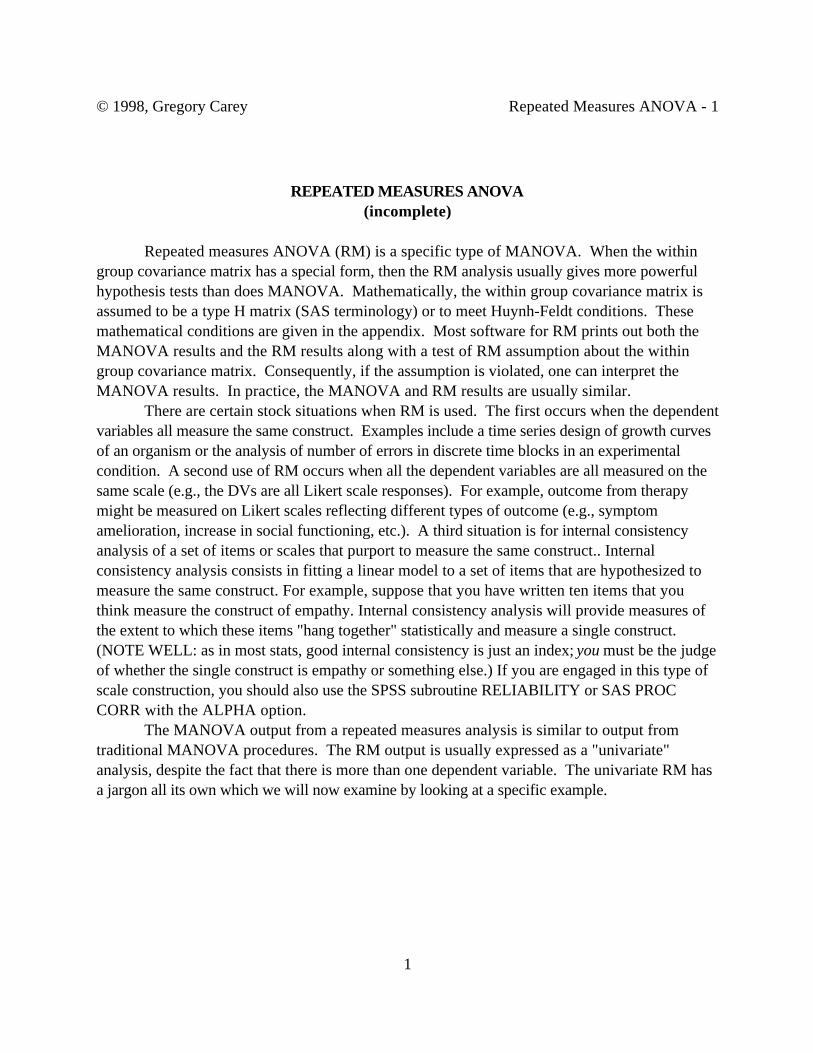
The mean total test score for the experimental group (170.5) is greater than the mean total testscore for controls (154.4). The difference is significant (t = -2.04, df = 58, p < .05) so we shouldconclude that the experimental language instruction is overall superior to the traditional languageinstruction.

There is nothing the matter with this analysis. It gives an answer to the major questionposed by the research design and suggests that in the future, the experimental method should beadopted for foreign language instruction.

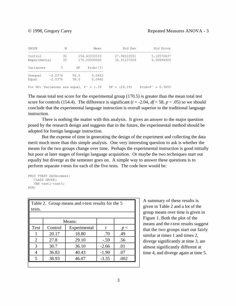
But the expense of time in generating the design of the experiment and collecting the datamerit much more than this simple analysis. One very interesting question to ask is whether themeans for the two groups change over time. Perhaps the experimental instruction is good initiallybut poor at later stages of foreign language acquisition. Or maybe the two techniques start outequally but diverge as the semester goes on. A simple way to answer these questions is toperform separate t-tests for each of the five tests. The code here would be:

PROC TTEST DATA=rmex1; CLASS GROUP; VAR test1-test5;RUN;

A summary of these results isgiven in Table 2 and a lot of thegroup means over time is given inFigure 1. Both the plot of themeans and the t-test results suggestthat the two groups start out fairlysimilar at times 1 and times 2,diverge significantly at time 3, arealmost significantly different attime 4, and diverge again at time 5.

Table 2. Group means and t-test results for the 5tests.

Means:Test Control Experimental t p <

1 20.17 18.80 .70 .492 27.8 29.10 -.59 .563 30.7 36.10 -2.66 .014 36.83 40.43 -1.90 .075 38.93 46.07 -3.35 .002


4

This analysis gives more insight, but leads to its own set of problems. We have performed 5different significance tests. If these tests were independent—and they are clearly norindependent because they were performed on the same set of individuals—then we should adjustthe α level by a Bonferroni formula

α adjustednumber of tests= − = − =1 95 1 95 01

12. . .. .

Using this criterion, we would conclude that the differences in test 3 are barely significant, thosein test 4 are not significant, while the means for the last test are indeed different. Perhaps themajor reason why the two groups differ is only on the last exam in the course.

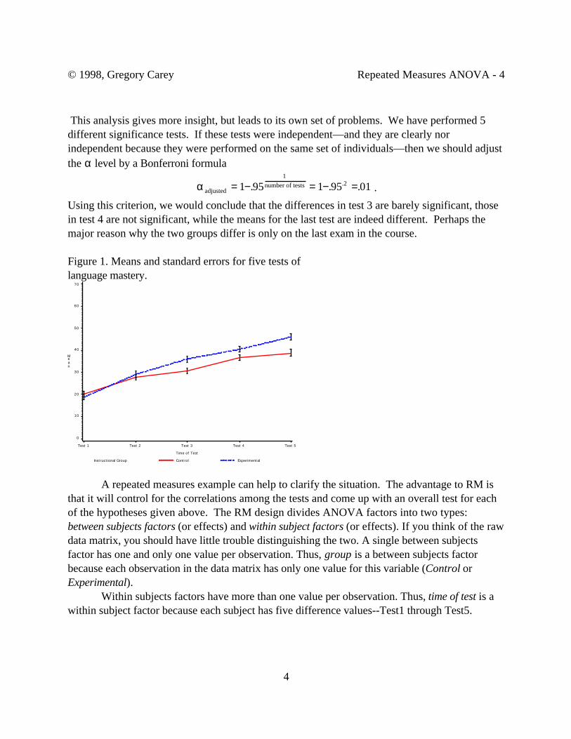
Figure 1. Means and standard errors for five tests oflanguage mastery.

Instructional Group Control Experimental

Mean

0

10

20

30

40

50

60

70

Time of Test

Test 1 Test 2 Test 3 Test 4 Test 5

A repeated measures example can help to clarify the situation. The advantage to RM isthat it will control for the correlations among the tests and come up with an overall test for eachof the hypotheses given above. The RM design divides ANOVA factors into two types:between subjects factors (or effects) and within subject factors (or effects). If you think of the rawdata matrix, you should have little trouble distinguishing the two. A single between subjectsfactor has one and only one value per observation. Thus, group is a between subjects factorbecause each observation in the data matrix has only one value for this variable (Control orExperimental).

Within subjects factors have more than one value per observation. Thus, time of test is awithin subject factor because each subject has five difference values--Test1 through Test5.


5

Another way to look at the distinction is that between subject factors are all the independentvariables. Within subject factors involve the dependent variables. All interaction terms thatinvolve a within subject factor are included in within subject effects. Thus, interactions of time oftest with group is a within subject effect. Interactions that include only between subject factorsare included in between subjects effects.

The effects in a RM ANOVA are the same as those in any other ANOVA. In the presentexample, there would be a main effect for group, a main effect for time and an interaction betweengroup and time. RM differs only in the mathematics used to compute these effects.

At the expense of putting the cart before the horse, the SAS commands to perform therepeated measures for this example are:

TITLE Repeated Measures Example 1;PROC GLM DATA=rmex1; CLASS group; MODEL test1-test5 = group; MEANS group; REPEATED time 5 polynomial / PRINTM PRINTE SUMMARY;RUN;

As in an ANOVA or MANOVA, the CLASS statement specifies the classificationvariable which is group in this case. The MODEL statement lists the dependent variables (onthe left hand side of the equals sign) and the independent variables (on the right hand side). TheMEANS statement asks that the sample size, means, and standard deviations be output for thetwo groups.

The novel statement in this example is the REPEATED statement. Later, this statementwill be discussed in detail. The current REPEATED statement gives a name for the repeatedmeasures or within subjects factor—time in this case—and the number of levels of that factor—5in this example because the test was given over 5 time periods. The word polynomial instructsSAS to perform a polynomial transform of the 5 dependent variables. Essentially this creates 4“new” variables from the original 5 dependent variables. (Any transformation of k dependentvariables will result in k - 1 new transformed variables.) The PRINTM option prints thetransformation matrix, the PRINTE option prints the error correlation matrix and some otherimportant output, and the SUMMARY option prints ANOVA results for each of the fourtransformed variables.

Usually it is the transformation of the dependent variables that gives the RM analysisadditional insight into the data. Transformations will be discussed at length later. Here we justnote that the polynomial transformation literally creates 4 new variables from the 5 originaldependent variables. The first of the new variables is the linear effect of time; it tests whetherthe means of the language mastery tests increase or decrease over time. The second new variable


6

is the quadratic effect of time. This new variable tests whether the means have a single “bend” tothem over time. The third new variable is the cubic effect over time; this tests for two “bends” inthe plot of means over time. Finally the fourth new variable is the quartic effect over time, and ittests for three bends in the means over time.

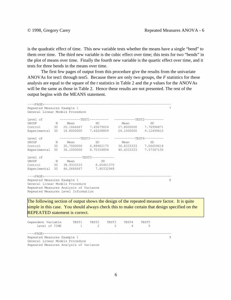
The first few pages of output from this procedure give the results from the univariateANOVAs for test1 through test5. Because there are only two groups, the F statistics for theseanalysis are equal to the square of the t statistics in Table 2 and the p values for the ANOVAswill be the same as those in Table 2. Hence these results are not presented. The rest of theoutput begins with the MEANS statement.

---<PAGE>-------------------------------------------------------------------Repeated Measures Example 1 7General Linear Models Procedure

Level of -----------TEST1---------- -----------TEST2----------GROUP N Mean SD Mean SDControl 30 20.1666667 7.65679024 27.8000000 7.76996871Experimental 30 18.8000000 7.46208809 29.1000000 9.12499410

Level of -----------TEST3---------- -----------TEST4----------GROUP N Mean SD Mean SDControl 30 30.7000000 6.88902175 36.8333333 7.06659618Experimental 30 36.1000000 8.70334854 40.4333333 7.57347155

Level of ------------TEST5------------GROUP N Mean SDControl 30 38.9333333 8.65401375Experimental 30 46.0666667 7.80332968

---<PAGE>-------------------------------------------------------------------Repeated Measures Example 1 8General Linear Models ProcedureRepeated Measures Analysis of VarianceRepeated Measures Level Information

Dependent Variable TEST1 TEST2 TEST3 TEST4 TEST5 Level of TIME 1 2 3 4 5

---<PAGE>-------------------------------------------------------------------Repeated Measures Example 1 9General Linear Models ProcedureRepeated Measures Analysis of Variance

The following section of output shows the design of the repeated measure factor. It is quitesimple in this case. You should always check this to make certain that design specified on theREPEATED statement is correct.


7

Partial Correlation Coefficients from the Error SS&CP Matrix / Prob > |r|

DF = 58 TEST1 TEST2 TEST3 TEST4 TEST5

TEST1 1.000000 0.451725 0.417572 0.510155 0.477928 0.0001 0.0003 0.0010 0.0001 0.0001

TEST2 0.451725 1.000000 0.445295 0.599058 0.493430 0.0003 0.0001 0.0004 0.0001 0.0001

TEST3 0.417572 0.445295 1.000000 0.650573 0.465271 0.0010 0.0004 0.0001 0.0001 0.0002

TEST4 0.510155 0.599058 0.650573 1.000000 0.493323 0.0001 0.0001 0.0001 0.0001 0.0001

TEST5 0.477928 0.493430 0.465271 0.493323 1.000000 0.0001 0.0001 0.0002 0.0001 0.0001

TIME.N represents the nth degree polynomial contrast for TIME

M Matrix Describing Transformed Variables TEST1 TEST2 TEST3 TEST4 TEST5TIME.1 -.6324555320 -.3162277660 0.0000000000 0.3162277660 0.6324555320TIME.2 0.5345224838 -.2672612419 -.5345224838 -.2672612419 0.5345224838TIME.3 -.3162277660 0.6324555320 -.0000000000 -.6324555320 0.3162277660TIME.4 0.1195228609 -.4780914437 0.7171371656 -.4780914437 0.1195228609

E = Error SS&CP MatrixTIME.N represents the nth degree polynomial contrast for TIME TIME.1 TIME.2 TIME.3 TIME.4TIME.1 1723.483333 -2.521377 236.550000 313.306091TIME.2 -2.521377 2187.726190 98.502728 35.622692TIME.3 236.550000 98.502728 1657.950000 -468.112779

These are the partial correlations for the dependent variables controlling for all the independentvariables in the model. They are printed because the PRINTE option was specified and theyanswer the question, "To what extent is Test1 correlated with Test2 within each of the twogroups?" Many of these correlations should be significant. Otherwise, there is really no sense indo repeated measures analysis—just do separate ANOVA on each dependent variable.

Below is the transformation matrix. It is printed here because the PRINTM option wasspecified in the REPEATED statement. Because we specified a POLYNOMIALtransformation, this matrix gives coefficients for what are called orthogonal polynomials. Theyare analogous but not identical to contrast codes for independent variables. The first newvariable, TIME.1, gives the linear effect over time, the second, TIME.2 is the quadratic effect,etc.


8

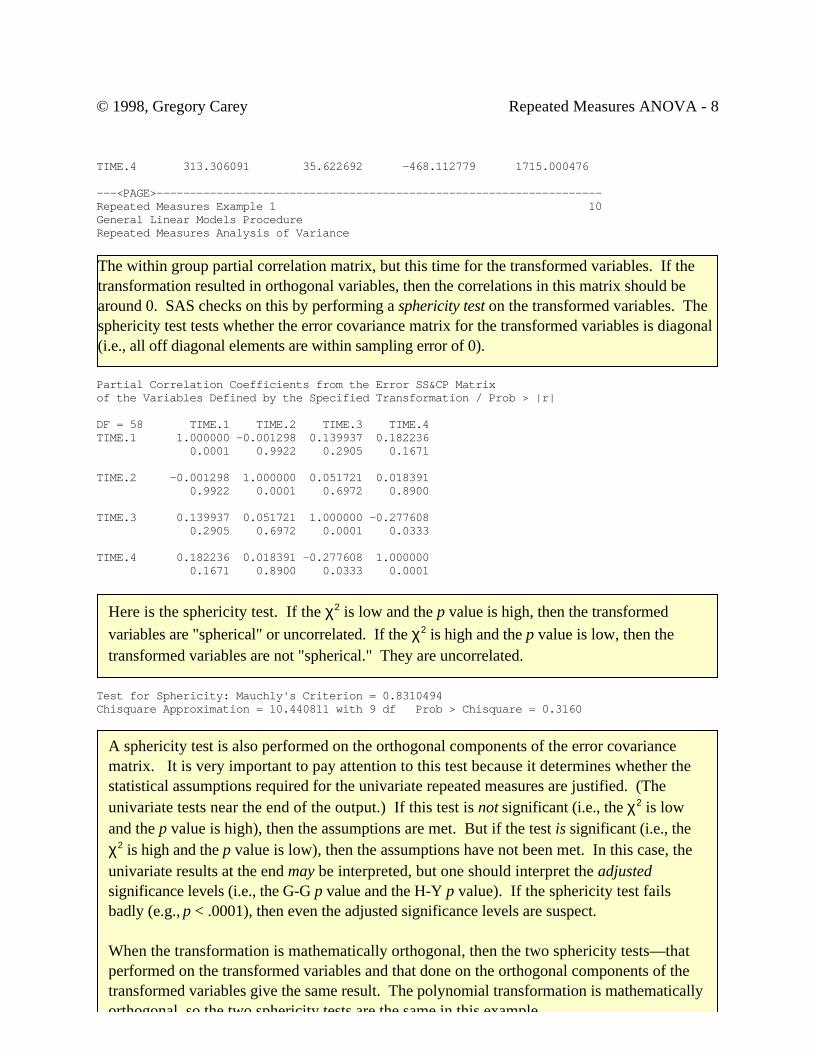
TIME.4 313.306091 35.622692 -468.112779 1715.000476


Partial Correlation Coefficients from the Error SS&CP Matrixof the Variables Defined by the Specified Transformation / Prob > |r|

DF = 58 TIME.1 TIME.2 TIME.3 TIME.4TIME.1 1.000000 -0.001298 0.139937 0.182236 0.0001 0.9922 0.2905 0.1671

TIME.2 -0.001298 1.000000 0.051721 0.018391 0.9922 0.0001 0.6972 0.8900

TIME.3 0.139937 0.051721 1.000000 -0.277608 0.2905 0.6972 0.0001 0.0333

TIME.4 0.182236 0.018391 -0.277608 1.000000 0.1671 0.8900 0.0333 0.0001

Test for Sphericity: Mauchly's Criterion = 0.8310494Chisquare Approximation = 10.440811 with 9 df Prob > Chisquare = 0.3160

The within group partial correlation matrix, but this time for the transformed variables. If thetransformation resulted in orthogonal variables, then the correlations in this matrix should bearound 0. SAS checks on this by performing a sphericity test on the transformed variables. Thesphericity test tests whether the error covariance matrix for the transformed variables is diagonal(i.e., all off diagonal elements are within sampling error of 0).

Here is the sphericity test. If the χ2 is low and the p value is high, then the transformedvariables are "spherical" or uncorrelated. If the χ2 is high and the p value is low, then thetransformed variables are not "spherical." They are uncorrelated.

A sphericity test is also performed on the orthogonal components of the error covariancematrix. It is very important to pay attention to this test because it determines whether thestatistical assumptions required for the univariate repeated measures are justified. (Theunivariate tests near the end of the output.) If this test is not significant (i.e., the χ2 is lowand the p value is high), then the assumptions are met. But if the test is significant (i.e., theχ2 is high and the p value is low), then the assumptions have not been met. In this case, theunivariate results at the end may be interpreted, but one should interpret the adjustedsignificance levels (i.e., the G-G p value and the H-Y p value). If the sphericity test failsbadly (e.g., p < .0001), then even the adjusted significance levels are suspect.

When the transformation is mathematically orthogonal, then the two sphericity tests—thatperformed on the transformed variables and that done on the orthogonal components of thetransformed variables give the same result. The polynomial transformation is mathematicallyorthogonal, so the two sphericity tests are the same in this example.


9

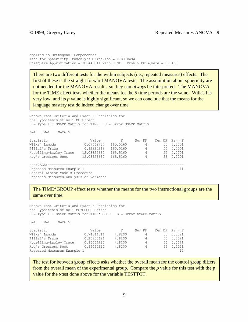
Applied to Orthogonal Components:Test for Sphericity: Mauchly's Criterion = 0.8310494Chisquare Approximation = 10.440811 with 9 df Prob > Chisquare = 0.3160

Manova Test Criteria and Exact F Statistics forthe Hypothesis of no TIME EffectH = Type III SS&CP Matrix for TIME E = Error SS&CP Matrix

S=1 M=1 N=26.5

Statistic Value F Num DF Den DF Pr > FWilks' Lambda 0.07669737 165.5260 4 55 0.0001Pillai's Trace 0.92330263 165.5260 4 55 0.0001Hotelling-Lawley Trace 12.03825630 165.5260 4 55 0.0001Roy's Greatest Root 12.03825630 165.5260 4 55 0.0001


Manova Test Criteria and Exact F Statistics forthe Hypothesis of no TIME*GROUP EffectH = Type III SS&CP Matrix for TIME*GROUP E = Error SS&CP Matrix

S=1 M=1 N=26.5

Statistic Value F Num DF Den DF Pr > FWilks' Lambda 0.74044314 4.8200 4 55 0.0021Pillai's Trace 0.25955686 4.8200 4 55 0.0021Hotelling-Lawley Trace 0.35054260 4.8200 4 55 0.0021Roy's Greatest Root 0.35054260 4.8200 4 55 0.0021Repeated Measures Example 1 12

There are two different tests for the within subjects (i.e., repeated measures) effects. Thefirst of these is the straight forward MANOVA tests. The assumption about sphericity arenot needed for the MANOVA results, so they can always be interpreted. The MANOVAfor the TIME effect tests whether the means for the 5 time periods are the same. Wilk's l isvery low, and its p value is highly significant, so we can conclude that the means for thelanguage mastery test do indeed change over time.

The TIME*GROUP effect tests whether the means for the two instructional groups are thesame over time.

The test for between group effects asks whether the overall mean for the control group differsfrom the overall mean of the experimental group. Compare the p value for this test with the pvalue for the t-test done above for the variable TESTTOT.


10

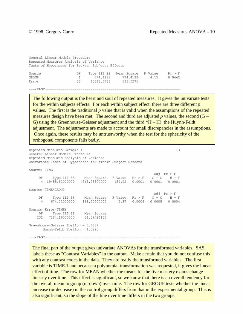
General Linear Models ProcedureRepeated Measures Analysis of VarianceTests of Hypotheses for Between Subjects Effects

Source DF Type III SS Mean Square F Value Pr > FGROUP 1 774.4133 774.4133 4.15 0.0462Error 58 10818.5733 186.5271

---<PAGE>-------------------------------------------------------------------

Repeated Measures Example 1 13General Linear Models ProcedureRepeated Measures Analysis of VarianceUnivariate Tests of Hypotheses for Within Subject Effects

Source: TIME Adj Pr > F DF Type III SS Mean Square F Value Pr > F G - G H - F 4 19455.82000000 4863.95500000 154.92 0.0001 0.0001 0.0001

Source: TIME*GROUP Adj Pr > F DF Type III SS Mean Square F Value Pr > F G - G H - F 4 674.02000000 168.50500000 5.37 0.0004 0.0005 0.0004

Source: Error(TIME) DF Type III SS Mean Square 232 7284.16000000 31.39724138

Greenhouse-Geisser Epsilon = 0.9332 Huynh-Feldt Epsilon = 1.0225

---<PAGE>-------------------------------------------------------------------

The following output is the heart and soul of repeated measures. It gives the univariate testsfor the within subjects effects. For each within subject effect, there are three different pvalues. The first is the traditional p value that is valid when the assumptions of the repeatedmeasures design have been met. The second and third are adjusted p values, the second (G –G) using the Greenhouse-Geisser adjustment and the third *H – H), the Huynh-Feldtadjustment. The adjustments are made to account for small discrepancies in the assumptions. Once again, these results may be untrustworthy when the test for the sphericity of theorthogonal components fails badly.

The final part of the output gives univariate ANOVAs for the transformed variables. SASlabels these as "Contrast Variables" in the output. Make certain that you do not confuse thiswith any contrast codes in the data. They are really the transformed variables. The firstvariable is TIME.1 and because a polynomial transformation was requested, it gives the lineareffect of time. The row for MEAN whether the means for the five mastery exams changelinearly over time. This effect is significant, so we know that there is an overall tendency forthe overall mean to go up (or down) over time. The row for GROUP tests whether the linearincrease (or decrease) in the control group differs from that in the experimental group. This isalso significant, so the slope of the line over time differs in the two groups.


11

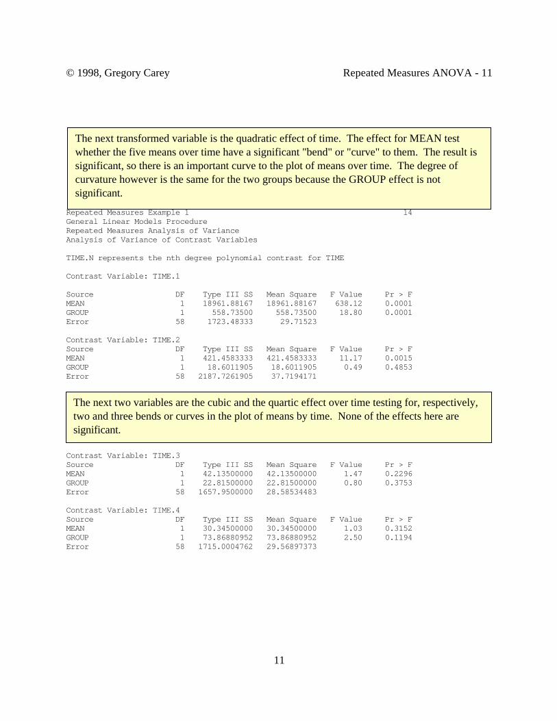
Repeated Measures Example 1 14General Linear Models ProcedureRepeated Measures Analysis of VarianceAnalysis of Variance of Contrast Variables

TIME.N represents the nth degree polynomial contrast for TIME

Contrast Variable: TIME.1

Source DF Type III SS Mean Square F Value Pr > FMEAN 1 18961.88167 18961.88167 638.12 0.0001GROUP 1 558.73500 558.73500 18.80 0.0001Error 58 1723.48333 29.71523

Contrast Variable: TIME.2Source DF Type III SS Mean Square F Value Pr > FMEAN 1 421.4583333 421.4583333 11.17 0.0015GROUP 1 18.6011905 18.6011905 0.49 0.4853Error 58 2187.7261905 37.7194171



The next transformed variable is the quadratic effect of time. The effect for MEAN testwhether the five means over time have a significant "bend" or "curve" to them. The result issignificant, so there is an important curve to the plot of means over time. The degree ofcurvature however is the same for the two groups because the GROUP effect is notsignificant.

The next two variables are the cubic and the quartic effect over time testing for, respectively,two and three bends or curves in the plot of means by time. None of the effects here aresignificant.


12

Factorial Within Subjects EffectsThe example given above had only a single within subjects factor, the time of the test.

Other designs, however, may have more than a single within subjects effect. As an example,consider a study aimed at testing whether an experimental drug improves the memories ofAlzheimer patients2. Thirty patients were randomly assigned to three treatment groups: (1)placebo or 0 milligrams (mg) of active drug, (2) 5 mg of drug, and (3) 10 mg. The memory taskconsisted of two modes of memory (Recall vs Recognition) on two types of things remembered(Names versus Objects) with two frequencies (Rare vs Common). That is, the patients weregives a list consisting of Rare Names (Waldo), Rare Objects (14th century map), Common Names(Bill), and Common Objects (fork) to memorize. The ordering of these four categories within alist was randomized from patient to patient. Half the patients within each drug group were asked to recall as many things on the list as they could. The other half were asked to recognize as manyitems as possible from a larger list. A new list was presented to the patients, and the oppositetask was performed. That is, those who had the recall task were given the recognition task, andthose initially given the recognition task were required to recall. Assume that previous researchwith this paradigm has shown that there are no order effects for the presentation. (Thisassumption is for simplicity only--it could easily be modeled using more advanced techniquesthan repeated measured.) The dependent variables are "memory scores." High scores indicatemore items remembered. Table 3 gives the design.

Table 3. Design of a study evaluating the influence of an experimental drug on memory inpatients with Alzheimer's disease.

Recall RecognitionNames Objects Names Objects

Obs. Drug Rare Comm Rare Comm Rare Comm Rare Comm1 1 63 70 73 76 68 81 77 902 1 72 74 68 70 76 87 82 94. . . . . . . . . .

30 3 80 85 78 87 88 92 94 103

There is one between subject's factor, the dose of drug. It has three levels—no active drug, 5 mg

2 The data are fictitious. The program for analysis may be found in the file~carey/p7291dir/alzheimr.sas


13

of drug, and 10 mg of drug. There are three within subjects factors. The first is memory modewith two levels, recall and recognition; the second is type of item recalled with the two levels ofnames and objects; and the third is the frequency of the item recalled with the two levels of rareor common.

In terms of ANOVA factors, a repeated measures design has the same logical structure asregular ANOVA. Hence, we can look on this design as being a 3 x 2 x 2 x 2 ANOVA. TheANOVA factors are drug, memory mode, type, and frequency. The ANOVA will fit maineffects for all four of these factors, all two way interactions (e.g., drug*memory mode,drug*type, etc.), all of the three way interactions (e.g., drug*memory mode*type), and the fourway interaction. Every ANOVA effect that contains at least one within subjects factor isconsidered a within subject's effect. Hence, the interaction of drug*type is a within subjectseffect as well as the interaction of drug*type*frequency.

Transformations: Why Do Them?The primary reason for transforming the dependent variables in RM is to generate

variables that are more informative than the original variables. Consider the RM example. Thedependent variables are tests of language mastery. Scores on a mastery test should be low early inthe course and increase over the course. At some point, we might expect them to asymptote,depending upon the difficulty of the mastery test. We can then reformulate the researchquestions into the following set of questions: Do some types of instruction increase mastery at afaster rate than other types? Does computer based instruction increase mastery at a faster ratethan classroom instruction? To answer these questions, we want to compare the independentvariables on the linear increase over time in mastery test scores. If the mastery test is constructedso that scores asymptote at some time point during the course, we could ask the followingquestions: Do some types of instructions asymptote faster than other types? Or, does computerbased instruction asymptote faster than classroom instruction? To answer these questions, wewant to test the differences in the quadratic effect over time for the independent variables. Inshort, we want to transform the test scores so that the first transformed variable is the lineareffect over time and the second variable is the quadratic effect over time. We can then do aMANOVA or RM on the transformed variables.

Transformations: How to Do ThemBoth SAS and SPSS recognize that constructing transformation matrices is a real pain in


14

the gluteus to the max. Thus, they do it for you. As a user of a RM design, your major obligationis to choose the transformation that makes the most sense for your data. Be very careful,however, is using automatic transformations in statistical packages. There is no consensusterminology, so what is called a "contrast" transformation in one package may not be the same asa "contrast" transformation in another package. Always RTFM3! SAS will automaticallyperform the following transformations for you:

CONTRAST. A CONTRAST transformation compares each level of the repeated measureswith the first level. It is useful when the first level represents a control or baseline level ofresponse and you want to compare the subsequent levels to the baseline. For our example, thefirst transformed variable will be the (Test1 - Test2), the second transformed variable will be(Test1 - Test3), the third (Test1 - Test4) and the last (Test1 - Test5). CONTRAST is thedefault transformation in SAS--the one you get if you do not specify a transformation.

MEAN. A MEAN transformation compares a level with the mean of all the other levels. It ismostly useful if you haven't the vaguest idea of how to transform the repeated measuresvariables. For the example, the first transformed variable will be (Test1 - mean of [Test2 + Test3+ Test4 + Test5]), the second variable will be (Test2 - mean of [Test1 + Test3 + Test4 +Test5]), etc. Note that there is always one less transformation than the number of variables.Hence, if you use a MEAN transform in SAS, you will not get the last level contrasted with themean of the other levels. If you have a burning passion to do this, see the PROC GLMdocumentation in the SAS manual.

PROFILE. A PROFILE transformation compares a level against the next level. It is sometimesuseful in testing responses that are not expected to increase or decrease regularly over time. Forthe example, the first transformed variable is (Test1 - Test2), the second is (Test2 - Test3), thethird is (Test3 - Test4), etc.

HELMERT. A HELMERT transform compares a level to the mean of all subsequent levels. Thisis a very useful transformation when one wants to pinpoint when a response changes over time.For our example, the first transformed variable would be (Test1 - mean of [Test2 + Test3 +Test4 + Test5]), the second would be (Test2 - mean of [Test3 + Test4 + Test5]), the thirdwould be (Test3 - mean of [Test4 + Test5]), and the last would simply be (Test4 - Test5). If the

3 For those who have not encountered the acronym RTFM, R stands for Read, T stands forThe, and M stands for Manual.


15

univariate F statistics were significant for the first and second transformed variables but notsignificant for the third and fourth, then we would conclude that language mastery was achievedby the time of the third test.

POLYNOMIAL. A POLYNOMIAL transform fits orthogonal polynomials. Like a Helmerttransform, this is useful to pinpoint changes in response over time. It is also useful when therepeated measures are ordered values of a quantity, say the dose of a drug. The first transformedvariable represents the linear effect over time (or dose). The second transformed variable denotesthe quadratic effect, the third the cubic effect, etc. If you are familiar enough with polynomials tointerpret the observed means in light of linear, quadratic, cubic, etc. effects, this is anexceptionally useful transformation. Often, one can predict beforehand the order of thepolynomial but not the exact time period where the response might be maximized (or minimized).

SPSS will also transform repeated measures variables using the CONTRAST subcommand to theMANOVA procedure. Note, however, that terminology and procedures differ greatly betweenSAS and SPSS. Be particularly careful of the CONTRAST statement. In SAS, the CONTRASTstatement refers to a transformation of only the independent variables. The CONTRAST optionon the REPEATED statement allows for a specific type of transformation for repeated measuresvariables. SPSSx views a CONTRAST as a transformation of either independent variables ordependent variables, depending upon the context. To make the issue more confusing, SPSSx hasanother subcommand, TRANSFORM, that applies only to the dependent variables. Also, bothpackages will do a "profile" transformation, but actually do different transformations. You shouldalways consult the appropriate manual before ever transforming the repeated measuresvariables. Always RTFM!

Quick and Dirty Approach to Repeated Measures

Background: There are probably as many different ways to perform repeated measures analysisas there are roads that lead to Rome. Furthermore, there are just as many differences interminology. Here the term "repeated measures" is used synonymously with "within subjects."Thus, within subjects factors are the same as repeated measures factors. Also note that the SASuse of a "contrast" transformation for repeated measures is not the same as contrast coding astaught by Chick and Gary. Here, the term "transformation" is used to refer to the creation of newdependent variables from the old dependent variables. [Sorry about all this but I did not make upthe rules.] The following is one quick and dirty way to perform a repeated measures ANOVA (or


16

regression). There are several other ways to accomplish the same task, so there is no "right" or"wrong" way as long as the correct model is entered and the correct statistics interpreted.


17

Setting up the data and the SAS commands

1. Make certain the data are entered so that each row of the data matrix is an independentobservation. That is, if Abernathy is the first person, belongs to group 1, and has three scoresover time (11, 12, and 13). Then enter

Abernathy 1 11 12 13

and not

Abernathy 1 1 11Abernathy 1 2 12Abernathy 1 3 13

It is possible to do a repeated measures analysis with the same person entered as many times asthere are repeats of the measures, but that type of analysis will not be explicated here.

2. Use GLM and use the model statement as if you were doing a MANOVA. All repeatedmeasures variables are the dependent variables. Suppose the three scores are called SCORE1,SCORE2, and SCORE3 in the SAS data set and GROUP is the independent variable. Then use

PROC GLM; CLASSES GROUP;MODEL SCORE1 SCORE2 SCORE3 = GROUP;

3. Use the REPEATED statement to indicate that the dependent variables are repeated measuresof the same construct or, if you prefer the other terminology, within subjects factors. Arecommended statement is

REPEATED <name> <number of levels> <transformation> / PRINTMPRINTE SUMMARY;

where <name> is a name for the measures (or within subject factors), <number of levels> givesthe number of levels for the factor, and <transformation> is the type of multivariatetransformation. For our example,


18

REPEATED TIME 3 POLYNOMIAL / PRINTM PRINTE SUMMARY;

will work just fine.

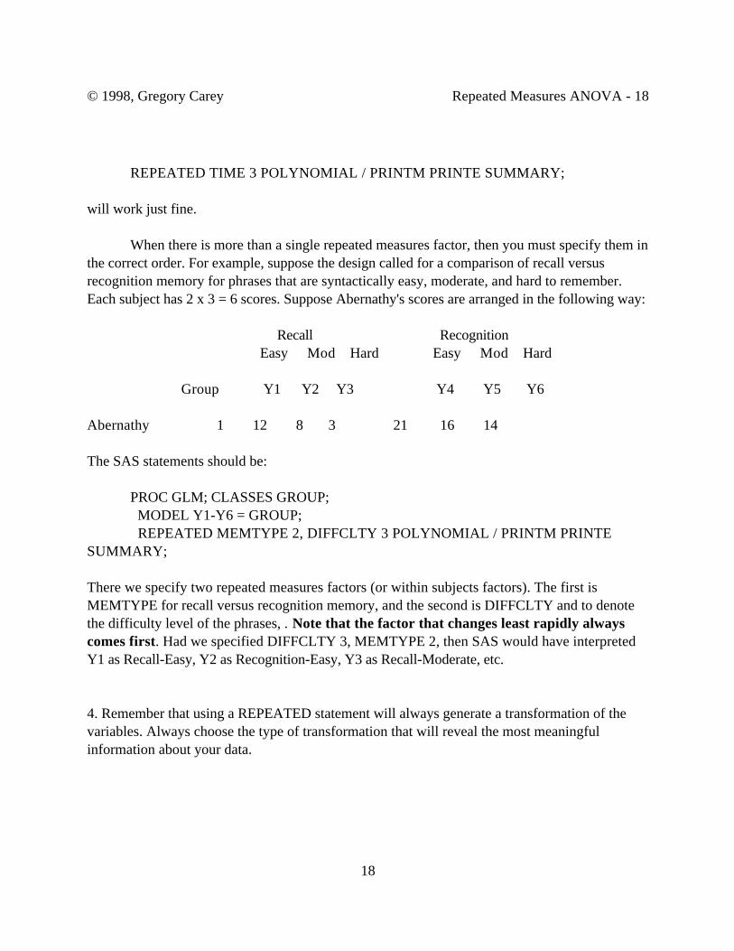
When there is more than a single repeated measures factor, then you must specify them inthe correct order. For example, suppose the design called for a comparison of recall versusrecognition memory for phrases that are syntactically easy, moderate, and hard to remember.Each subject has 2 x 3 = 6 scores. Suppose Abernathy's scores are arranged in the following way:

Recall RecognitionEasy Mod Hard Easy Mod Hard

Group Y1 Y2 Y3 Y4 Y5 Y6

Abernathy 1 12 8 3 21 16 14

The SAS statements should be:

PROC GLM; CLASSES GROUP; MODEL Y1-Y6 = GROUP; REPEATED MEMTYPE 2, DIFFCLTY 3 POLYNOMIAL / PRINTM PRINTE

SUMMARY;

There we specify two repeated measures factors (or within subjects factors). The first isMEMTYPE for recall versus recognition memory, and the second is DIFFCLTY and to denotethe difficulty level of the phrases, . Note that the factor that changes least rapidly alwayscomes first. Had we specified DIFFCLTY 3, MEMTYPE 2, then SAS would have interpretedY1 as Recall-Easy, Y2 as Recognition-Easy, Y3 as Recall-Moderate, etc.

4. Remember that using a REPEATED statement will always generate a transformation of thevariables. Always choose the type of transformation that will reveal the most meaningfulinformation about your data.


19

5. That is all there is to doing a repeated measures ANOVA or Regression. You can use theCONTRAST statement if you wish to contrast code categorical independent variables. Just makecertain that you place the CONTRAST statement before the REPEATED statement.

Interpreting the Output

This is a synopsis of the handout on Repeated Measures. You should follow these stepsto interpret the output.

1. The first thing SAS writes in the output is the design for the repeated measures. Always checkthis to make certain that correctly specified the levels of the repeated measures. This isparticularly important when there is more than a single within subjects factor.

2. The second thing to check is whether error covariance matrix can be orthogonally transformed.The tests of sphericity will tell you that. Some transformations in SAS are deliberately set up tobe orthogonal (e.g., POLYNOMIAL with no further qualifiers); other transformations are notorthogonal (e.g., CONTRAST). If a transformation is orthogonal, then SAS will print out onetest of sphericity. If a transformation is not orthogonal, then SAS spits out two tests ofsphericity. The first test is for the straight transformation. The second test is for the orthogonalcomponents of the transformation. In this case, it is the second test--the one for the orthogonalcomponents--that you want to interpret.

3. If the χ2 test for sphericity is not significant, then ignore all the MANOVA output andinterpret the RM ANOVA results for the within subjects effects. These are labelled in the SASoutput as "Univariate Tests of Hypotheses for Within Subjects Effects."

4. If the χ2 test for sphericity was very significant, then you can interpret the MANOVA resultsor the adjusted probability levels from Greenhouse-Geisser and the Huynh-Feldt corrections forthe within subjects effects. If is often a good idea to compare the MANOVA significance withthe Greenhouse-Geisser and the Huynh-Feldt adjusted significance levels to make certain there isagreement between them.

5. The between subjects effects are not affected by the results of the sphericity test. Hence, SASoutput with the heading "Tests of Hypotheses for Between Subjects Effects" will always becorrect.


20

6. Always interpret the output for the transformed variables. It can often tell you somethingimportant about the data. Exactly what it tells you will depend upon the type of transformationyou used in the REPEATED statement.

7. Always make certain that the raw means and standard deviations are printed. If you have notgotten them in the GLM procedure with the MEANS statement, then get them by using PROCMEANS, PROC UNIVARIATE, or PROC SUMMARY. Repeated measures or within subjectsdesigns are useless when the results are not interpreted with respect to the raw data.

Appendix 1: Mathematical Assumptions of RM analysisThere are two major assumptions required for RM analysis. The first of these is that the

within group covariance matrices are homogeneous. That means that the covariance matrix forgroup 1 is within sampling error of the covariance matrix of group 2 which is within samplingerror of the covariance matrix of group 3, etc. for all groups in the analysis. Programs such asSPSS permit a direct test of homogeneity of covariance matrices. Much to the dismay of manySAS enthusiasts, testing for homogeneity of covariance must be done in a roundabout way. Toperform such an analysis, create a new variable, say, group, that has a unique value for eachgroup in the analysis. For example, suppose that you have a 2 (sex) by 3 (treatment) factorialdesign. The data are in a SAS data set called wacko where sex is coded as 1 = male, 2 = femaleand the 3 categories of treatment are numerically coded as 1, 2, and 3. Then a new variable calledgroup may be generated using the following code

DATA wacko2; SET wacko; group = 10*sex + treatmnt;RUN;

The second step is to perform a discriminant analysis using group as the classificationvariable, the RM variables as the discriminating variables, and the METHOD=NORMAL andPOOL=TEST options in the PROC DISCRIM statement. If the RM variables in data set wackowere vara, varb, and varc, then the SAS code would be

PROC DISCRIM DATA=wacko2 METHOD=NORMAL POOL=TEST; CLASS group; VAR vara varb varc;RUN;


21

Pay attention only to the results of the test for pooling the within group covariance matrices andignore all the other output.

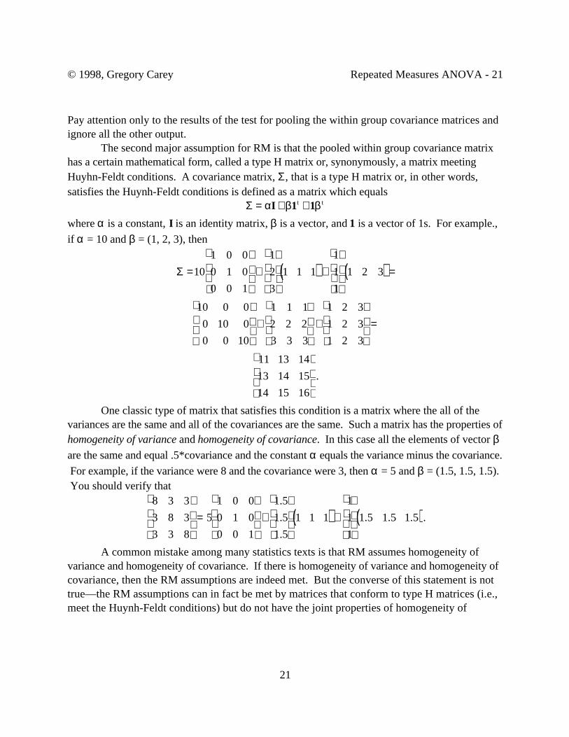
The second major assumption for RM is that the pooled within group covariance matrixhas a certain mathematical form, called a type H matrix or, synonymously, a matrix meetingHuyhn-Feldt conditions. A covariance matrix, Σ, that is a type H matrix or, in other words,satisfies the Huynh-Feldt conditions is defined as a matrix which equals

Σ = β βαI 1 1+ +t t

where α is a constant, I is an identity matrix, β is a vector, and 1 is a vector of 1s. For example.,if α = 10 and β = (1, 2, 3), then

Σ =10

1 0 0

0 1 0

0 0 1

+1

2

3

1 1 1( ) +1

1

1

1 2 3( ) =

10 0 0

0 10 0

0 0 10

+1 1 1

2 2 2

3 3 3

+1 2 3

1 2 3

1 2 3

=

11 13 14

13 14 15

14 15 16

.

One classic type of matrix that satisfies this condition is a matrix where the all of thevariances are the same and all of the covariances are the same. Such a matrix has the properties ofhomogeneity of variance and homogeneity of covariance. In this case all the elements of vector βare the same and equal .5*covariance and the constant α equals the variance minus the covariance. For example, if the variance were 8 and the covariance were 3, then α = 5 and β = (1.5, 1.5, 1.5). You should verify that

8 3 3

3 8 3

3 3 8

= 5

1 0 0

0 1 0

0 0 1

+1.5

1.5

1.5

1 1 1( ) +1

1

1

1.5 1.5 1.5( ).

A common mistake among many statistics texts is that RM assumes homogeneity ofvariance and homogeneity of covariance. If there is homogeneity of variance and homogeneity ofcovariance, then the RM assumptions are indeed met. But the converse of this statement is nottrue—the RM assumptions can in fact be met by matrices that conform to type H matrices (i.e.,meet the Huynh-Feldt conditions) but do not have the joint properties of homogeneity of


22

variance and homogeneity of covariance.

repeated measures anova...

Documents