replenishment policies for retail pharmacies in emerging

Replenishment Policies for Retail Pharmacies in Emerging Markets by

Kevin Kwan Yu Chu Honors Bachelor of Science in Biological Chemistry, University of Toronto, Canada, 2011

and

Juan Manuel Martínez Pizano Bachelor of Science in Industrial Engineering, Instituto Tecnológico de Santo Domingo, Dominican

Republic, 2016

SUBMITTED TO THE PROGRAM IN SUPPLY CHAIN MANAGEMENT IN PARTIAL FULFILLMENT OF THE REQUIREMENTS FOR THE DEGREE OF

MASTER OF APPLIED SCIENCE IN SUPPLY CHAIN MANAGEMENT AT THE

MASSACHUSETTS INSTITUTE OF TECHNOLOGY

JUNE 2019

© 2019 Kevin Chu and Juan Manuel Martínez Pizano. All rights reserved. The authors hereby grant to MIT permission to reproduce and to distribute publicly paper and electronic

copies of this capstone document in whole or in part in any medium now known or hereafter created.

Signature of Author: ____________________________________________________________________ Kevin Kwan Yu Chu

Department of Supply Chain Management May 10, 2019

Signature of Author: ____________________________________________________________________

Juan Manuel Martínez Pizano Department of Supply Chain Management

May 10, 2019 Certified by: __________________________________________________________________________

Dr. Christopher Mejía Argueta Director, MIT SCALE Latin America Network

Capstone Advisor

Accepted by: _________________________________________________________________________

Dr. Yossi Sheffi Director, Center for Transportation and Logistics Elisha Gray II Professor of Engineering Systems Professor, Civil and Environmental Engineering

3

Replenishment Policies for Retail Pharmacies in Emerging Markets by

Kevin Kwan Yu Chu Juan Manuel Martínez Pizano

Submitted to the Program in Supply Chain Management on May 10, 2019 in Partial Fulfillment of the

Requirements for the Degree of Master of Applied Science in Supply Chain Management

ABSTRACT

Pharmaceuticals account for over hundreds of billions of dollars of the global annual healthcare expenditure. Inventory management is essential for the financial health of the retail pharmaceutical industry. The retail pharmacy studied in this research, faced a challenge managing high-performance inventory policies. This capstone project aims to determine how a set of replenishment policies can help maintain efficient inventory levels and minimize undesired effects of non-centralized discounts and stock-outs in the stores. Our analysis is based on descriptive analytics such as demand frequency, variability, level and profit, data mining and quantitative models such as inventory control, sensitivity analysis and scenario analysis on forecast horizon, stock-out penalty, and customer service level to determine the replenishment policies best suited for the group of prioritized SKUs analyzed. The analyzed policies demonstrate the tradeoff between leveraging supplier-pushed discounts and the increased costs of excess inventory. In addition, the tradeoff between reducing holding costs and controlling stock-out penalties is analyzed. From the SKUs analyzed the research suggests using the (Q, R) policy for high profit SKUs for an average of 33% cost reduction and (s, S) policy for low profit SKUs for an average of 37% cost reduction.

=

Capstone Advisor: Dr. Christopher Mejía Argueta Title: Director, MIT SCALE Latin America Network

4

ACKNOWLEDGMENTS

We thank the sponsoring company for giving the team all the data needed to complete the project. Special thanks to the company’s CEO for all the support given to the team. Also, the IT team that helped us obtain the extra data needed to continue with our research. We are glad to be part of these innovative Master program that gave us the opportunity to continue our learning from online with the MicroMasters to on-campus. I would like to thank my partner Kevin for the great effort and enthusiasm he put into this project. I would also thank our advisor Dr. Chris Mejía for the continuous support, interest in the project and constructive feedback. My future wife Daniela for being there when I needed it the most in this important journey. My parents for encouraging me to make this dream come true. My friends for their support. Finally, the whole SCM classmates that made this learning experience knowledgeable and fun.

Juan It was an honor to work on this project alongside Juan, my capstone partner, for his patience, insights and enthusiasm throughout the process. To our advisor, Dr. Chris Mejía, I would like to express my gratitude for his support and guidance. I would also like to thank my family for their support along this journey. Finally, to the entire SCM class of 2019, I thank you all for making this adventure a wonderful and enjoyable one. I wish you all the best of luck in your future endeavors.

Kevin

5

Replenishment Policies for Retail Pharmacies in Emerging Markets

Table of Content

1 Introduction ..................................................................................................................................... 8

2 Literature Review .......................................................................................................................... 12

3 Methodology ................................................................................................................................. 16

3.1 Process Mapping .................................................................................................................... 16

3.2 Stakeholders ........................................................................................................................... 17

3.3 Data Collection ...................................................................................................................... 18

3.4 Descriptive Analysis............................................................................................................... 19

3.5 Assumptions and Conditions .................................................................................................. 21

3.5.1 Assumptions ................................................................................................................... 21

3.5.2 Conditions ...................................................................................................................... 21

3.6 Cost function formulation ....................................................................................................... 22

3.6.1 Notation ......................................................................................................................... 22

3.6.1.1 Parameters .................................................................................................................. 22

3.6.1.2 Variables .................................................................................................................... 22

3.6.2 Total Cost Function at DC .............................................................................................. 25

3.6.3 Total Cost Function at a Retail Store ............................................................................... 25

3.7 Inventory management formulation ........................................................................................ 26

3.7.1 Periodic review replenishment policy .............................................................................. 26

3.7.2 Continuous review replenishment policy ......................................................................... 26

3.7.3 Sensitivity Analysis ........................................................................................................ 27

4 Case study: A retail pharmacy chain in emerging markets .............................................................. 29

4.1 Company description .............................................................................................................. 29

4.2 Problem description ................................................................................................................ 30

4.3 Demand and inventory analysis .............................................................................................. 30

5 Results ........................................................................................................................................... 34

5.1 Cost structure ......................................................................................................................... 34

5.2 Periodic review replenishment policy ..................................................................................... 36

5.3 Continuous review replenishment policy ................................................................................ 38

5.4 Scenario and sensitivity analysis ............................................................................................. 40

5.5 Managerial insights and recommendations .............................................................................. 42

6 Conclusions and future work .......................................................................................................... 44

References ............................................................................................................................................. 46

6

APPENDIX A Sensitivity Analysis Using Four Different Forecast Horizons ...................................... 48

APPENDIX B Sensitivity Analysis Using Four Different Cycle Service Levels ................................. 49

APPENDIX C Sensitivity Analysis Using Four Different Stock-Out Penalty Factors ......................... 50

7

List of Figures

Figure 1. Methodology .......................................................................................................................... 16 Figure 2. Process Information Flow ....................................................................................................... 17 Figure 3. Process Physical Flow ............................................................................................................. 17 Figure 4. Goodness of Fit of DC Aggregated Demand Normal Distribution ........................................... 28 Figure 5. Goodness of Fit of Store Demand Poisson Distribution ........................................................... 28 Figure 6. Logistics network of the sponsor company .............................................................................. 29 Figure 7. 2x2 matrix: Demand Frequency vs Profit ................................................................................ 31 Figure 8. Demand level vs Average Transaction .................................................................................... 32 Figure 9. Demand Variability vs Average Transaction ........................................................................... 33 Figure 10. Average Product Cost Component as a Percentage of Total Costs ......................................... 35 Figure 11. Cost Breakdown of (Q, R) periodic review inventory model .................................................. 35 Figure 12. Cost Breakdown of (s, S) continuous review inventory model ............................................... 36 Figure 13. Effect of (Q, R) Replenishment Policy on Cost Components ................................................. 37 Figure 14. Effect of (Q, R) Replenishment Policy on CSL and Average Cost per Unit ............................ 38 Figure 15. Effect of (s, S) Replenishment Policy on Cost Components ................................................... 39 Figure 16. Effect of (s, S) Replenishment Policy on CSL and Average Cost per Unit.............................. 39 Figure 17. Savings per SKU for each inventory model ........................................................................... 40

List of Tables

Table 1. Sensitivity Analysis of SKU 01 ................................................................................................ 42

8

1 Introduction

Pharmaceuticals account for over $600 billion USD of the annual global healthcare expenditure

(Plunkett Research Group, 2019). In fact, global prescription drugs and over-the-counter (OTC) therapy

sales in 2016 were around $768 billion USD (Evaluate, 2018). Drugs are commonly dispensed through

retail pharmacies and hospitals. They can be expensive to store, handle and distribute due to inaccurate,

non-effective inventory management that could create stock-outs, shortages of essential medicines,

inappropriate handling and excessive costs due to high inventory levels and urgent shipments to avoid lost

sales. This project will focus on retail pharmacies and on inventory management.

Inventory management is an important task in retail companies as inventory is often one of the

biggest investments and total current assets, which helps companies keeping a high level of service and be

more responsive to demand variability. Pharmaceuticals may not want to cut inventory, given that their

margins are higher too. Nevertheless, current inventory levels are high, and the industry could free up $25

billion USD if it reduced inventories on hand (Keeling, Lösch & Schrader, 2010). Publicly traded

companies’ annual reports for major retailers such as Walgreens (Walgreens Boots Alliance Inc., 2019),

CVS (CVS Health Corporation, 2019), Walmart (Walmart Inc., 2019) and Target (Target Corporation,

2019) show that inventory accounts for around one-third of total current assets.

However, having too much inventory can cause financial difficulties due to the impact on cash

flow, but carrying too little can lead to stock-outs and backorders, which can lead to lost sales. Some of the

undesired effects of high inventory levels are inefficient supply chains, high demand variability, and

pushed-inventory, reactive policies. Also, marketing strategies such as supplier-pushed promotions can

increase inventory or decrease it to negative numbers when not properly managed.

Since inventory is easy to acquire in traditional pushed-inventory models, companies may fall into

the trap of carrying excess inventory at multiple echelons of the supply chain to help reduce stock-outs but

at the expense of negatively affecting the company’s finances. On the other hand, carrying low inventory

9

levels could condemn firms to having a low level of service, being unable to respond quickly to changes in

the demand or supply, and losing their customers. Having constant stock-out have a real impact on a

company’s sales, accounting for up to 50% of the total supply chain cost (Alicke, Ebel, Schrader & Shah,

2014). Sanches-Ruiz, Blanco & Kyguoliene, (2018) characterize the most common reactions customers

have towards stock-out events, finding that they can buy the product at other stores and just leave the store

and not buying the product.

A major difficulty in determining the right amount of inventory is the replenishment policy. How

much inventory should a specific store, or distribution center, carry before ordering more? How often

should these facilities be replenished and replenish associated stores? What is the effect that stock-out and

non-centralized discounts might have in the performance of the pharmaceutical retail chain? Factors such

as volume, frequency of orders in terms of level and variability, lead time, reorder point and safety stock

need to be analyzed. Understanding these factors will effectively meet demand and reduce the stock-out

probability, while still maintaining accurate inventory levels and managing stock holding points more

closely to reduce throughput times.

The sponsor firm is a pharmaceutical retail chain that located in an urban area from an emerging

region. Its logistics network is composed of a distribution center, over 50 stores nationwide and around 120

suppliers. Through different strategies such as early payment discounts and incremental volume discounts

pushed by its suppliers, the company has managed to raise its margin by 7% in a country whose government

regulates markups at 30% and prohibits vertical integration.

The company is in the top three firms of the pharmaceutical industry in the country. Despite its

high market share, the firm faces some challenges in terms of effectively managing its inventory levels to

increase product availability in the stores, optimize its replenishment policies, and define an efficient way

to manage discounts, promotions and reduce the probability of stock-out across its network and stores.

10

The key research questions that we aim to answer with this study is: How can the replenishment

policies of a retail pharmacy chain be improved to maintain efficient inventory levels and minimize

undesired effects of discounts and stock-outs to keep a sustainable high-performance operation?

We used existing literature and case studies to determine the state-of-the-art inventory management

techniques and models to reduce stock-out and undesired effects of discounts pushed by suppliers. The next

step was conducting process and stakeholder mapping to understand the whole supply chain network and

different processes of the retail pharmacy chain affecting product availability and thus determining accurate

inventory levels. Using the rich data sets collected from the company, we study the demand level, frequency

and the inventory records to understand patterns, drivers and trends via plots and descriptive, exploratory

statistics. This allowed us for applying models drawn from the existing literature to reduce the impact of

the identified drivers. Considering opportunities and challenges faced by the sponsor company, we

formulated a couple of inventory models based on a (Q, R) periodic review and a (s, S) continuous review

replenishment policies. Then, we evaluate them to define which replenishment policies best fit with the

company’s different products to optimize inventory levels of the SKUs to be analyzed under multiple

circumstances.

To analyze effects of the proposed replenishment policies, we also conducted a set of changes in

stock-out penalties and different values in the level of service. We also performed other scenario analyses

such as trying different SKU characteristics like demand frequency, demand level and profits to quantify

possible inventory factors such as holding costs and suppliers pushed discounts that may be affect

replenishment, availability of products and cause stock-outs and oscillations in the costs and times. By

analyzing four categories of products (i.e., 1) fast movers with high sales, 2) the fast movers with low sales,

3) slow movers with high sales, and 4) slow movers with low sales) from top suppliers at five stores, we

proposed periodic and continuous review models to optimize inventory levels, minimize undesired effects

of discounts and maintain long-term profitable operations for the company. For the sake of scope, we limit

our analysis to the retailer’s supply chain and no collaborative strategies with the suppliers are considered.

11

This paper demonstrates that establishing (Q, R) and (s, S) replenishment policies, to balance to

tradeoffs between supplier-pushed discounts, excess inventory, and stock-out penalties. The replenishment

policies analyzed had different impact on the analyzed parameters. The experiments resulted on average

estimated cost savings of 33% compared to the baseline for (Q, R) inventory model and an average of 37%

for the (s, S) model. These savings are mostly derived from the inventory reduction. While the team

observed savings, the service level was affected by an average of -2.53% for (Q, R) policy and an average

of -2.09% for the (s, S) policy compared to the baseline. Despite the reduced service level, the potential

savings are higher than the potential lost sales from stock-outs.

This document is organized as follows: In Section 2 the literature body that supports this capstone

project and its methodology is introduced. We also identify practical gaps and discuss practical

contributions. In Section 3, a detailed description of the methodology is presented. This includes an

explanation of the process mapping, the data collection and processing, the descriptive, exploratory

statistics and the quantitative approach based on two distinct replenishment policies. Then in Section 4,

problem description of the sponsor company is introduced, together with a description of the data sets and

descriptive, exploratory statistics regarding demand and inventory records. In Section 5, the results of the

replenishment policies for diverse SKUs of the retail pharmacy chain are analyzed in different scenarios

together with a sensitivity analysis. Finally, the conclusions and future work are summarized in Section 6.

12

2 Literature Review

Pharmaceuticals depend on a supply chain composed of manufacturers or importers, wholesalers,

and pharmacies in several distribution channels. Each of these echelons traditionally hold high levels of

inventory, causing a huge economic impact in the overall logistics network that sums up billions of dollars

in losses (Keeling et al. 2010; Wollenhaupt, 2018; Anand & Chadha, 2019). In average, a retail pharmacy

could turn over stock five to 12 times per year; however, there is a considerable demand variability in each

SKU that is linked to the season of the year. It is important not only to understand the stocking but also to

manage effectively the lead times to reach the store shelves (Wollenhaupt, 2018). Therefore, inventory can

become a competitive advantage or a nightmare.

High-performance replenishment policies from other industries have shown to be effective in

healthcare and pharmacy management systems (Nicholson, Vakharia, & Erenguc, 2004; Nematollahi,

Hosseini-Motlagh, & Heydari, 2017), healthcare-related products possess particular features (Saedi,

Kundakcioglu & Henry 2016). But the customization of inventory models and its related technologies

remains low in the retail pharmacy industry, mainly in emerging markets, where information is barely

available.

Given that some healthcare products are required to be always available in hospitals and pharmacies

(de Vries, 2011), regardless of the forecasted demand, a high-level-of-service approach should be followed

for these items over a cost-minimization approach. Consequently, pharmaceutical stock-outs could lead to

severe health complications at worse or be extremely costly (Wollenhaupt, 2018).

De Vries (2011) found some stakeholders, namely medical specialists, prioritized medical service

levels over inventory and materials management. Despite the support from procurement and logistics staff,

inventory projects were opposed by medical specialists based on conjecture regarding its value to patients

rather than data analysis. Thus, there is misalignment among stakeholders of the healthcare supply chains

has to be controlled. Also, inventory levels decisions in this type of supply chains are rarely data-driven

13

and they are often based on the experience of the staff (Nicholson et al. 2004). To change this, it is crucial

to set common objectives, determine key performance indicators (KPIs) associated with each role, align

incentives and make decision based on data (Simatupang & Sridharan, 2005).

In addition, it is crucial to study the two primary challenges of these supply chains (Vrata, 2012):

a) Lack of inventory visibility, which causes an increase in stock-outs and non-centralized

discount strategies.

b) Cost of inaccurate inventory levels, which comes from excessive stock or lost sales due to the

existence of backorders, shortages in the retailers.

To tackle these challenges, this research focuses on using data analytics and inventory modeling

tools to face the aforementioned challenges, while keeping profitable operations for the sponsor company.

Inventory inaccuracy is a supplementary factor that can lead to other difficulties such as over costs,

redundant inventory and unnecessary transfers among logistics facilities and stores (Shteren & Avrahami,

2017). Maintaining the correct inventory policies can increase the financial health of a company and even

open expansion possibilities. For instance, Zara, a fashion retail chain has succeeded by having a flexible

supply chain with fast replenishment policies of high demand products (Industria de Diseño Textil, 2019).

Even though, the apparel retail and pharma retail have some similarities, the latter requires more agile,

robust inventory solutions because it deals with patients, sick people and not with customers. The

pharmaceutical manufacturer GSK has changed its way to serve diverse retailers in order to avoid piling up

stock across the supply chain. These retail chains are now able to gain rapid visibility of the inventory levels

and timing throughout the network, which allows increasing effectiveness, reducing stock-out and

satisfying customer requirements timely (Wollenhaupt, 2018).

Kelle, Woosley, & Schneider (2012) created a framework to incorporate holding and ordering costs

into hospital inventory-management models, while Nicholson et al. (2004) found savings through

14

outsourcing inventory decisions for non-critical items. Establishment of a centralized offsite warehouse has

also demonstrated significant reduction in inventory costs (Cheng, & Whittemore, 2008).

Despite our study will not consider collaborative approaches between dyads of the healthcare

supply chain, we cite a couple of papers to prove that there is possible to improve several inventory-related

KPIs. Nematollahi et al. (2017) found that collaborative efforts between suppliers and hospitals resulted in

increased item fill rate and economic profitability of the entire supply chain. Similarly, Uthayakumar, &

Priyan (2013) developed a two-echelon inventory model to minimize costs through joint-optimization while

maintaining close to 100% customer service level (CSL).

Guerrero, Yeung, & Guéret (2013) went even further, exploring a multiple product, multi-echelon

model that combines much of these concepts. The model is focused on an (R, s, S) inventory policy with a

central pharmacy acting as a distribution center, and includes CSL, capacity concerns, possible emergency

deliveries, batching and ordering constraints with a joint-optimization approach. Despite the extensive

research, most focus on (s, S) models and none consider how promotional discounts from pharmacy

suppliers could affect inventory management decisions.

Promotional discounts can have a huge impact in demand variability and increase the bullwhip

effect significantly (O’Donnell, Maguire, McIvor, & Humphreys, 2007). However, if optimal ordering and

stocking policies for the specific set of conditions are defined, better results will be gotten. Despite there

are barely studies in pharmaceutical retail about managing inventory policies with promotional discounts;

applicable research can be found in other retail industries. Cárdenas-Barrón, & Sana (2015) explored how

such promotional discounts affected profit if both supplier, and retailer acted individually or collaboratively.

Also, Güder, Zydiak, Chaudhry (1994) explored how to apply multiple item ordering with incremental

discounts in order to minimize the total purchase cost.

In line with the joint-optimization models, collaborative efforts through cost sharing benefitted both

parties and maximized the supply channel. Expanding on the (Q, r) inventory policies, Saracoglu,

15

Topaloglu, & Keskinturk (2014) formulated a model incorporating a multi-period continuous review for

multiple products. While effective, the model does not consider safety stock, shortages and backordering.

To complement this model, we reviewed the model from Ghosh, Khanra, &Chaudhuri (2011), where partial

backordering was incorporated. This model assumes the customers are impatient and the limited supply is

highly perishable. While these models will not be effective for retail pharmacies, we will extract how

perishability and lost sales are modelled for this paper.

Based on this literature review, we identified the following gaps: a) Most of the existing literature

in pharmacy inventory management focuses on hospitals, b) There is only a handful papers and reports

about retail pharmacy for emerging markets and c) There is scarce research about how suppliers pushed

discounts into retail pharmacy chains and the effect in the replenishment policies.

In summary, the main contribution of this work is to fill the aforementioned gaps and build an

inventory management framework as a tool to guide the replenishment decision for the sponsor company.

To the best of our knowledge, while these models have been proven in hospital settings and other retail

industries, retail pharmacy application has not been explored. From the existing hospital research, we will

formulate a model based on the work of Guerrero et al. (2013). Building upon it, we will incorporate the

effect of promotional discounts. However, we will not pursue joint-optimization due to the lack of

comprehensive supplier data. Thus, our objective is to minimize costs for the retail pharmacy.

16

3 Methodology

This section gives the overview of our research methodology. Our research on inventory control in

hospital pharmacies and other retail industries was the basis for our choice of methodology: process

mapping, stakeholder mapping, data collection, descriptive analysis, and quantitative modeling. Figure 1

illustrates the major steps described below.

Figure 1. Methodology

3.1 Process Mapping

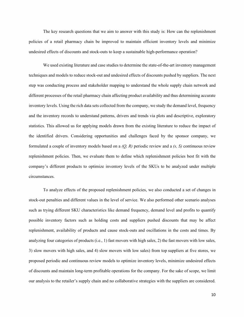
The company supply chain process is presented in two different flows: the information flow and

the physical product movement flow.

The information flow (Figure 2) starts when the demand is generated by sales. With the demand

data and other negotiation factors such as volume discounts, the Purchase Department (PD) negotiates the

terms with the suppliers. When the suppliers accept the terms, they deliver the products to the Distribution

Center (DC), where it is processed and made available for picking. The stores generate their orders

depending on demand and the effective inventory, and these are delivered depending on the inventory

availability in the DC. These orders are posted in the ERP and then sent to the store. The store receives the

transfer order, so the product is now available in the store. When a customer requires their need and if the

product is available, then an order receipt is created. With these receipts, the demand data is captured.

17

Figure 2. Process Information Flow

The physical product flow (Figure 3) starts when the product arrives at the DC with the supplier’s

invoice to verify the compliance between the units delivered and the units invoiced. Afterwards it goes

through a process to identify the expiration date. The products are then put away in the picking location, to

be picked when the store’s orders come in. After the physical picking is done, products are delivered to

stores. When stores receive the products and check the compliance between the order and the physical

delivery, the product is put away in the designated location to be sold. When customers require their needs

and after all the paperwork is done, the product is delivered to the customer. These processes can take a

minimum of 0.5 days up to 4 days, and an average of 1.5 days.

Figure 3. Process Physical Flow

3.2 Stakeholders

The most important stakeholders of the company’s different flows explained in the process

mapping are as follows.

Customer: The main objective of the company is to fulfill customers’ needs. The customer’s main concern

when going to a pharmacy is product availability and price. Since pharmacies differentiation is mostly

18

service not necessarily product selection, product availability is an important factor to maintain customer

frequency.

Shareholders: Inventory is one of the main assets of a company. It is less liquid than cash and carrying cost

is one of the important costs of the company. Therefore, lowering the inventory is away shareholders free

up cash. Also, service level is crucial because since customers care about the product availability, it drives

revenues, which also drives profit. Having a good balance between inventory levels and service level is

vital to maintain customer satisfaction and financial health.

Supplier: For suppliers, market share is one of their main drivers since it drives sales. For this reason,

suppliers are willing to give volume discounts, create product promotions and give samples to drive sales

at the POS. The benefits may be large but, these strategies need to be closely analyzed in order to not get

carried away and increase the company inventory levels unnecessarily.

Store Personnel: This personnel is the public face of the company. Having the product available and making

the customer happy is what the drives the store personnel. Their main goal is to have a high customer

satisfaction even if it means carrying higher inventory than necessary.

After determining the main stakeholders and their main drivers, we observe that inventory

management and replenishment policies are important to achieve the customer needs as well as inventory

reduction.

3.3 Data Collection

The team collected different sets of data to analyze. First, the team got the POS sales data for the

top 50 products with highest sales frequency. Also, the team received, through a business intelligence

software, the company sales figures. The POS data and the sales figures helped us understand the demand

behavior of these products and select products to analyze. We selected products with different

characteristics, such as high sales frequency - high sales volume, high sales frequency – medium sales

volume, medium sales frequency – high sales volume and medium sales frequency – medium sales volume.

19

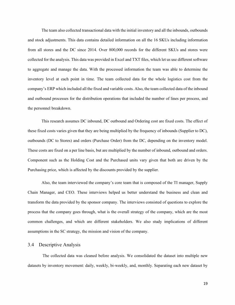
The team also collected transactional data with the initial inventory and all the inbounds, outbounds

and stock adjustments. This data contains detailed information on all the 16 SKUs including information

from all stores and the DC since 2014. Over 800,000 records for the different SKUs and stores were

collected for the analysis. This data was provided in Excel and TXT files, which let us use different software

to aggregate and manage the data. With the processed information the team was able to determine the

inventory level at each point in time. The team collected data for the whole logistics cost from the

company’s ERP which included all the fixed and variable costs. Also, the team collected data of the inbound

and outbound processes for the distribution operations that included the number of lines per process, and

the personnel breakdown.

This research assumes DC inbound, DC outbound and Ordering cost are fixed costs. The effect of

these fixed costs varies given that they are being multiplied by the frequency of inbounds (Supplier to DC),

outbounds (DC to Stores) and orders (Purchase Order) from the DC, depending on the inventory model.

These costs are fixed on a per line basis, but are multiplied by the number of inbound, outbound and orders.

Component such as the Holding Cost and the Purchased units vary given that both are driven by the

Purchasing price, which is affected by the discounts provided by the supplier.

Also, the team interviewed the company’s core team that is composed of the TI manager, Supply

Chain Manager, and CEO. These interviews helped us better understand the business and clean and

transform the data provided by the sponsor company. The interviews consisted of questions to explore the

process that the company goes through, what is the overall strategy of the company, which are the most

common challenges, and which are different stakeholders. We also study implications of different

assumptions in the SC strategy, the mission and vision of the company.

3.4 Descriptive Analysis

The collected data was cleaned before analysis. We consolidated the dataset into multiple new

datasets by inventory movement: daily, weekly, bi-weekly, and, monthly. Separating each new dataset by

20

SKU and facility, descriptive analysis was performed for each type of data (inventory movement, lead time,

processing time, and costs).

Each type of inventory movement (sales, purchases, transfers, and inventory adjustments) was

analyzed. For the DC, sales were the aggregated sales of the SKU in the entire supply chain. Based on the

total inventory movement for each time period (based on consolidation of the dataset), the beginning and

ending inventory levels were calculated. Movement types were compared to determine any anomalies in

sourcing behavior and to understand if the supplier-pushed discounts were influencing purchasing practices.

Sales data from the inventory movement datasets were combined with the SKU details datasets

and analyzed to establish demand characteristics of the SKU, such as trend, seasonality, drug form, active

ingredient, packaging, and therapeutic category. From this analysis, we formed SKU categories.

In addition, the inventory data was used to determine if there were any potential stock-outs. Using

the inventory levels and the sales data, we determined the number of times a product ran out of inventory

at the end of a business day. A comparison of these stock-out data sets to the inventory levels of the DC

was performed for the SKU in order to determine if stock-outs at the DC were in turn causing stock-outs at

the retail level.

Lead times of each SKU were analyzed for both suppliers to the DC as well as the DC to retail

locations. We sought to understand the distribution of the lead time datasets to determine the proper method

of incorporation into the quantitative model. Goodness of fit analysis was used to verify our findings. In

addition, suppliers were compared and the lead times for transferring products between two retail locations

were also analyzed.

We analyzed the processing times of each SKU at the DC. Like the lead times, we verified the

distribution of the datasets. The processing times for each SKU were compared to determine if the SKU

had any influence over the processing time. This analysis was used to build the quantitative model.

21

Using the inventory movement data and the collected cost metrics, we analyzed the costs of each

SKU. The cost/unit and each type of cost for each SKU was calculated. From this data, the total relevant

costs were calculated and compared. The total relevant cost was used as an initial analysis of whether

leveraging promotions was beneficial for the company.

3.5 Assumptions and Conditions

3.5.1 Assumptions

To build an appropriate quantitative model, it is important to define a set of assumptions that are

realistic and allow making the mathematical model actionable. For the proposed inventory models of this

study, we define the following short list of assumptions:

• There is only one distribution center.

• Backorders are not allowed.

• All purchases from suppliers are shipped to the DC.

• Supplier promotions are in the form of extra quantities provided in exchange of increasing orders

of a SKU.

• Supplier promotions give one unit of SKU for free for every rf units ordered.

• There are data available about the demand, although these are not always known.

• Lead times are constant from DC to Stores = 1 day from supplier to DC = 2 days.

• Replenishments from DC prioritize stores based on alphanumerical order. This can be organized

depending store demand or frequency.

• The company has a desired service level at the store level depending on the type of SKU.

3.5.2 Conditions

• There are multiple SKUs, which we cluster in four categories.

• All SKUs fall under one of the established SKU categories.

• One year consists of 12 months of 4 weeks of 7 days.

22

• The holding cost of inventory is 24% per annum and accrued daily.

• The DC processing time is included in the lead time.

• The DC processing cost is included in the DC inbound cost and the outbound cost.

• Suppliers have a 100% fill rate. Suppliers fill rate is out of scope.

• Stock-out penalty is equal to the SKU markup (30%) multiplied by a stock-out rate.

3.6 Cost function formulation

3.6.1 Notation

3.6.1.1 Parameters

𝐶"# = Inbound costs to DC

𝐶"$ = Outbound costs from DC

𝐶%# = Inbound costs to Stores

𝐶%%= Outbound costs to Stores

𝐶& = Order cost (set-up cost)

𝐷( = Demand at DC (Aggregated demand from all stores)

𝐷) = 𝐸[𝐷%]= Expected value of the demand per Store

𝐹. = Free Units

𝐶. = Catalog cost per unit

ℎ0= Holding fee Rate

𝐶1 =𝐶. ∗ ℎ0

𝜎((6 = Standard Deviation of Demand over Lead Time at the DC

𝜎)(6 = Standard Deviation of Demand over Lead Time at the Store

𝑞8 = Free Units per every rf Units Ordered.

𝑟8 = Units required for qf

𝑆 = Number of Stores

3.6.1.2 Variables

𝑂𝐶= Ordering Component

𝐻𝐶 = Holding cost component

23

𝐷𝐶# = Inbound DC Component

𝐷𝐶𝑜 = Outbound DC Component

𝑆# = Inbound Store Component

𝐷𝑆%% = Stock-out Penalty Component at the DC

𝐶𝑆%% = Stock-out Penalty Component at the Store

𝑃[𝑥 > 𝑄%] = Expected Units Short at Store

𝑃[𝑥 > 𝑄(] = Expected Units Short at DC

𝑃. = Purchased Units (Paid Units)

𝑃𝐶 = Purchasing Cost Component

𝑄( = Units Ordered at DC

𝑄) = Units Ordered at Store

𝑅( = Reorder Point at the DC

𝑅) = Reorder Point at the Store

𝑘 = Safety Stock Factor

TRC = Total Relevant Cost for Company

𝑇𝑅𝐶(E = Total Relevant Cost for DC

𝑇𝑅𝐶) = Total Relevant Cost for Stores

In the presence of supplier promotions in the form of a free unit per 𝑟8 units ordered, the order

quantity at the DC, 𝑄( can be broken down into two components, 𝑃. and 𝐹., paid units and free units,

in the equation below:

𝑄( = 𝑃. + 𝐹. (1)

Furthermore, 𝐹. is a function of 𝑃. as presented in the following equation:

𝐹. = GHI0JK ∗ 𝑞8 (2)

The amount of 𝐹. received is equal to the floor function of 𝑃. divided by 𝑟8 multiplied by 𝑞8, the

quantity of free units per 𝑟8. As we have assumed𝑞8is always either one or zero, the 𝐹. function can

24

be solved as if it is continuous, as any known integer result can be rounded after to the closest possible

𝐹. (Knuth, Castle, & Wheeler, 2006). Thus, we remove the floor function, creating Equation 3:

𝐹. =HI0J∗ 𝑞8 (3)

Substituting Equation 3 into Equation 1 creates Equation 4, which will serve as the basis of our

cost formulation:

𝑄( =𝑃. ∗ (1 +NJ0J) (4)

There are seven components to the relevant variable costs function: cycle and safety stock holding

cost (5), ordering cost (6), inbound handling costs at the DC (7), product cost (8), outbound handling

costs at the DC (processing and labor costs at DC, 9), inbound handling costs at the store (10), stock-

out penalty at the DC (11), and stock-out penalty at the store (12) (Nahmias, & Olsen, 2015).

𝐻𝐶 = 𝐶1 ∗ (HIP+ 𝑘𝜎((6) (5)

𝑂𝐶 =𝐶& ∗(QRQ

(6)

𝐷𝐶𝑖 = 𝐶"# ∗(QRQ

(7)

𝑃𝐶 = 𝐶. ∗ 𝑄( (8)

𝐷𝐶$ = 𝐶"$ ∗ ∑(URU

)%VW (9)

𝐷𝑆# = 𝐶%# ∗ ∑(URU

)%VW (10)

𝐷𝑆)) = 𝐶(% ∗(QRQ∗ 𝑃[𝑥 > 𝑄(] (11)

𝐶𝑆)) = 𝐶%% ∗ ∑(URU∗ 𝑃[𝑥 > 𝑄%])

W (12)

Unlike the EOQ formulation (Nahmias, & Olsen, 2015), the product cost is considered a relevant

cost as the total product costs will decrease as Q increases. Like Equation 3, under our assumptions,

Equation 8 can be assumed to be continuous for our purposes. Adding the seven relevant cost

components, with Equation 4 substituted in, together creates the total relevant cost function:

25

𝑇𝑅𝐶 = EX∗HIP

+ (Q∗(EYZ[E\)[(EI∗HI)

HI[]J∗^I_J

+ (𝐶"$ + 𝐶%#) ∗ ∑(URU

)%VW + 𝐷𝑆)) + 𝐶𝑆)) (13)

3.6.2 Total Cost Function at DC

At the DC level, inbound handling costs and stock-out penalties at a store level are not incurred.

While the sponsor considers no penalty is incurred for a stock-out at the DC, the proposed cost model

does need to be constrained to a service level in order to ensure enough stock is on hand to service the

stores. As such, 𝐶(% is assumed to be equal to 𝐶%% for this purpose. Therefore, the following equation

represents the DC cost function:

𝑇𝑅𝐶(E = EX∗HIP

+ (Q∗(EYZ[E\)[(EI∗HI)

HI[]J∗^I_J

+ 𝐶"$ ∗ ∑(URU

)W + 𝐶%% ∗

(QRQ∗ 𝑃[𝑥 > 𝑄(] (14)

Taking the first derivative and solving for Pu* gives the optimal order size for the DC:

𝑃.∗ = `P∗(EYZ[E\)∗(∗0JEX∗(NJ[0J)

∗ `1 + Eaa∗H[bcRQ]EYZ[E\

(15)

Using Equation 4 with Equation 15, we can determine 𝑄(∗.

3.6.3 Total Cost Function at a Retail Store

The total cost function at the retail store level is composed of three relevant cost components: store

stock-out costs, inbound costs at the store, and holding costs (see Equation 16).

𝑇𝑅𝐶) =𝐶)) ∗(URU∗ 𝑃[𝑥 > 𝑄%] + (𝐶"$ + 𝐶%#)

(URU+EX∗RU

P (16)

Unlike the cost function at the DC, product cost is not a relevant cost as there are no discounts to

leverage in the internal transfer. By calculating the first derivative, then solving for 𝑄%∗, the optimal order

size or store replenishment, we form Equation 17:

𝑄%∗ = `P∗(EYd[EaZ)∗(aEX

∗ `1 + Eaa∗H[bcRU]EYd[EaZ

(17)

26

3.7 Inventory management formulation

In our experiments, the total of ending inventory and in transit inbound inventory per day is analyzed

to determine if an order is placed from the store to the DC or from the DC to the supplier, depending on the

lead time. The reorder point is set by the type of inventory policy used. For shipments from the DC to stores,

inventory is transferred to a transit location for the duration of the lead time to account for holding costs

during the shipment. This also ensures inventory promised to one store is not also promised to another store.

Also, it ensures that the inventory is not allocated immediately from the DC to the store.

Instance from the sponsor company were run using real historical demand data as well as randomized

demand data based on the observed demand distribution. The demand data from the DC is the sum of

demand across all stores.

3.7.1 Periodic review replenishment policy

The typical periodic review model is the (Q, R) replenishment policy that extrapolates the 𝑄(∗ and

Qs* from the cost model formulation, while 𝑅( and 𝑅) is determined with the following equations:

𝑅( = 𝑘𝜎((6 (18)

𝑅) = 𝑘𝜎)(6 (19)

The experimentation uses a periodic review model, where if the sum of any day’s ending inventory

and pending inbound inventory is less than R, Q units are ordered. This inventory policy would be useful

for low variability, low frequency products (Wadhwa, Bibhushan, & Chan, 2009). The fixed ordering

quantity would align the EOQ and the reorder point with the demand level.

3.7.2 Continuous review replenishment policy

The (s, S) inventory policy uses 𝑅( and 𝑅) as the DC and store values of s respectively, while S is

the summation of Q and R of the (Q, R) inventory policy (Nahmias, S. & Olsen, T.L., 2015), as shown

below:

27

𝑆( = 𝑅( + 𝑄( (20)

In the (s, S) inventory model, each DC or store will review the ending inventory daily. If the total

ending inventory and pending inbound inventory is less than s, an order is placed to replenish the DC or

store to inventory level S. In theory, this policy is useful for high-variability SKUs (Wadhwa et al., 2009).

The ordering quantity will be adjusted according to actual consumption, allowing the company to manage

better its variability. By comparing the (s, S) replenishment policy with the (Q, R) policy, the company can

determine the variability threshold where one policy is more beneficial than the other.

3.7.3 Sensitivity Analysis

Using the sponsor’s existing forecasting method, we calculated 𝑄(∗ and 𝑄%∗ using the annual, monthly,

biweekly and weekly forecasts. By analyzing various forecast horizons, we determine the effect of forecast

aggregation on the robustness of the analyzed replenishment policies.

As the sponsor company is not sure how to penalize the existence of stock-out, we performed a series

of sensitivity analyses at stock-out penalty factors 0, 2, 5, and 10. The stock-out costs were determined by

the stock-out penalty multiplied by the stock-out penalty factor. The values of 0, 2, 5, and 10, were chosen

to reflect the varying likelihoods of customers accepting backorders or leaving for a competitor depending

on SKU category. Given that computing this likelihood is out of the scope of the current project, we

proposed these values to analyze low, most likely and high values.

Similarly, safety factor k also underwent a sensitivity analysis. In order to observe the tradeoff between

total relevant cost and number of stock-outs, we experimented with 𝑃[𝑥 > 𝑄%] and 𝑃[𝑥 > 𝑄(] at levels of

significance equal to 99%, 95%, 90% and 85%, respectively. 𝑃[𝑥 > 𝑄%] and 𝑃[𝑥 > 𝑄(] were determined

based on the specific SKU’s demand distribution (i.e., Normal and Poisson, Figures 4 and 5). The values

of 99%, 95%, 90% and 85% were chosen as high CSL is a core strategy for the sponsor and the sponsor

wanted to analyze the associated costs for this strategy.

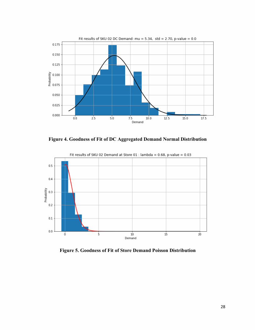
28

Figure 4. Goodness of Fit of DC Aggregated Demand Normal Distribution

Figure 5. Goodness of Fit of Store Demand Poisson Distribution

29

4 Case study: A retail pharmacy chain in emerging markets

4.1 Company description

The sponsor firm is a pharmaceutical retail chain located in urban areas from an emerging region.

The company in a region with an average income level of $350 USD per month per person. The population

density is around 11,000 people per square kilometer. The retail pharmacy chain has stores in areas with

the highest income and with the lowest income. It mainly concentrates its operations in the most densely

populated areas. Its logistics network is composed of a distribution center, over 50 stores nationwide and

around 120 suppliers (Figure 6).

Figure 6. Logistics network of the sponsor company

The company has accounted for a considerable amount of revenue in the last years and managed to

raise its margin by 7%. Despite the margin increase providing a net profit above the retail pharmacy industry

average, there is still room for improvement in building high-performance inventory policies.

The firm operates in a country whose government regulates markups at 30% (i.e., 23.08% gross

margin). The government also prohibits vertical integration between importers and pharmacies to motivate

30

purchases from local suppliers. The latter implies another challenge for the sponsor company that needs to

work closely with its suppliers and manage properly its inventory levels.

4.2 Problem description

The sponsor company has experienced challenges to manage its high inventory levels to guarantee

product availability in stores and across the supply chain. At the time of this analysis, the company counted

over 72 days of inventory. The company desires to have 45 or fewer days of inventory. According to

Inventory Management Result Survey from Tompkins International, (2018), the average number of days of

inventory on hand for the pharmaceutical and drug industry is 57.8 Days of Inventory Outstanding (DIO).

Also, benchmarking with the biggest retail pharmacy chains from the US, we can calculate that Walgreens

Boots Alliance, Inc. has approximately 34.2 DIO and CVS Health Corporation has around 35.2 DIO took

from their annual report.

These levels of inventory are driven by inefficiencies in the demand analysis, the inability to send single

units or partial blister packs from the distribution center (DC) to stores, and the procurement strategy for

the DC. As the company is having constant stock-outs at the DC and the store level, the procurement

strategy has opportunities for improvement. The company has tried aggregating demand to reduce

variability but has not managed to maintain efficient inventory levels. Also, a weighted average of sales

determines the replenishment policies, but it has not managed to increase product availability in stores due

to stock-outs at the DC.

A key challenge for the firm is to build inventory policies considering the effect that promotional

discounts pushed by suppliers insert into the retail pharmacy’s operations. Another challenge is to reduce

the number of stock-out across its network and stores.

4.3 Demand and inventory analysis

The team performed the analysis of 16 SKUs with very different demand characteristics. The

characteristics selected were demand frequency, demand level, demand variability, and profit based on

31

Cheng and Whittemore (2018). For all these analyses we performed graphical relationship among different

pairs of parameters such as: Profit vs Demand Frequency, Average Weekly Demand vs Average Demand

Frequency, Coefficient of Variation of Weekly Transaction vs Average weekly Transaction. These analyses

helped the team understand and differentiate the SKUs that were analyzed. These characteristics helped the

team differentiate the SKU demand patterns and identify which replenishment policy is better for each SKU

type. Also, the analyses support gaining knowledge about the impact that multiple parameters have in the

efficiency of the inventory models.

Figure 7. 2x2 matrix: Demand Frequency vs Profit

Figure 7 is normalized to be represented in a 2 x 2 matrix comparing demand frequency and gross

profit generation. This matrix helped the team understand the SKUs demand patterns on a standardized

32

scale. We used a normalized graph to be able to show how multiple SKUs might be categorized in fast and

slow movers as well as in high- and low-demand SKUs.

Figure 8. Demand level vs Average Transaction

Figure 8 is not normalized, and it represents the actual values of the average weekly transactions

vs the average weekly demand for each product. Figure 8 also helped the team understand the real demand

and selling frequency of each of the SKUs. The chart was useful to interpret the demand volume of each of

the SKUs.

33

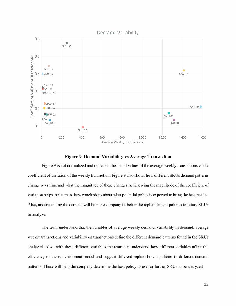
Figure 9. Demand Variability vs Average Transaction

Figure 9 is not normalized and represent the actual values of the average weekly transactions vs the

coefficient of variation of the weekly transaction. Figure 9 also shows how different SKUs demand patterns

change over time and what the magnitude of these changes is. Knowing the magnitude of the coefficient of

variation helps the team to draw conclusions about what potential policy is expected to bring the best results.

Also, understanding the demand will help the company fit better the replenishment policies to future SKUs

to analyze.

The team understand that the variables of average weekly demand, variability in demand, average

weekly transactions and variability on transactions define the different demand patterns found in the SKUs

analyzed. Also, with these different variables the team can understand how different variables affect the

efficiency of the replenishment model and suggest different replenishment policies to different demand

patterns. These will help the company determine the best policy to use for further SKUs to be analyzed.

34

5 Results

This section presents the results of the couple of inventory models analyzed under multiple

circumstance that are useful for the sponsor company. The team performed simulations using a periodic

and a continuous review inventory model. Then, the team explain the variety of potential impacts these

replenishment policies might bring to the company. Sensitivity analysis was performed using four different

forecast horizon, four different cycle service level and four different stock-out rate penalties for the 16

SKUs under study. This sensitivity analysis helps to understand the impact in the total costs and inventory

levels by changing each parameter at once with multiple values.

5.1 Cost structure

In all SKUs in both replenishment policies, the largest cost component are the product costs. They

accounted for close to or over 90% of the total costs (Figure 10). Aside from the product costs, the next

largest cost component is the retail store holding costs, consisting of 40% to 60% of the remainder (see

Figure 10 & 11). Retail store holding costs have a larger part of the total costs in SKUs with lower sales

frequency and higher profits. We found that most SKUs have lower holding costs under the (s, S) inventory

policy because the ordered quantity incorporates the on-hand inventory at the time the order is placed. In

contrast, the (Q, R) replenishment policy did not consider the on-hand inventory, leading to smaller sizes

and lower holding costs at both DC and retail.

As such, the most impactful cost components were product costs and the various holding costs, but

there is a tradeoff between these two components (Figures 10 and 11). Minimizing the average product

costs per unit by leveraging the supplier-pushed discounts will increase the overall holding costs. This was

driven by the increased order sizes needed to take advantage of the supplier-pushed discounts, but the

resulting increased inventory levels also increased holding costs.

35

Figure 10. Average Product Cost Component as a Percentage of Total Costs

Figure 11. Cost Breakdown of (Q, R) periodic review inventory model

14%

1%

48%

14%

1%

15%

8%

14%

2%

56%

12%

1%

11%6%

12%

2%

42%

15%

1%

18%

10%14%

1%

43%

15%

1%

17%

9%

0%

10%

20%

30%

40%

50%

60%

% DC HoldingCost

% TransitHolding Cost

% Store HoldingCost

% Ordering Cost % DC InboundCost

% DC OutboundCost

% Store InboundCost

(Q,R) % Operating Cost Over Total Operating Cost

SKU 02 SKU 07 SKU 08 SKU 13

Average Product Cost as % of Total CostSKU 02 86.24%SKU 07 91.97%SKU 08 92.00%SKU 13 91.71%

50.00%55.00%60.00%65.00%70.00%75.00%80.00%85.00%90.00%95.00%

Perc

ent o

f Tot

al C

ost

SKU

Average Product Cost Compenent


36

Figure 12. Cost Breakdown of (s, S) continuous review inventory model

The analyzed SKUs demonstrated the operating costs breakdown shown in Figures 11 and 12 for

the (Q, R) periodic review and (s, S) continous review inventory models, respectively. By removing the

product costs, it suggested the holding costs was the main driver and other cost components (ordering

cost, inbound and outbound costs) were insignificant.

5.2 Periodic review replenishment policy

For this inventory model, we found that overall it outperforms current company’s replenishment

policy. Changing the company’s replenishment policy to a (Q, R) – (Q, R) had an average cost reduction of

33%, but the effect on individual SKUs differed depending on the SKU characteristics. In general, SKUs

with higher profit performed better with the (Q, R) model. Holding costs at the DC level increased for all

SKUs, but significantly more for SKUs with lower profits (Figure 13). This held true for the retail stores,

with SKUs with high profits that benefited from reduced holding costs. The lowered total costs also had

increased average cost per unit and decreased CSL compared to the baseline (Figure 14), with high profit

SKUs experiencing a greater CSL decrease, but a lower increase of average cost per unit. This suggested

13%

1%

46%

14%

1%

17%

9%13%

1%

59%

11%

1%

10%5%

12%

2%

41%

15%

1%

19%

10%12%

1%

40%

16%

1%

20%

11%

0%

10%

20%

30%

40%

50%

60%

70%

% DC HoldingCost

% TransitHolding Cost

% Store HoldingCost

% Ordering Cost % DC InboundCost

% DC OutboundCost

% Store InboundCost

(s,S) % Operating Cost Over Total Operating Cost


37

the costs of placing larger orders to leverage the supplier-pushed discounts and maintaining a high CSL

may outweigh the resulting benefits.

Figure 13. Effect of (Q, R) Replenishment Policy on Cost Components

-150.00%-100.00%

-50.00%0.00%

50.00%100.00%150.00%200.00%250.00%300.00%350.00%

DC Holding C

ost

Tran

sit Holding C

ost

Store Holding C

ost

Orderin

g Cost

DC In

bound Cost

DC Outbound Cost

Store In

bound Cost

Product

Cost

Total Costs

Chan

ge (%

of B

asel

ine)

Cost Compenent

(Q, R) Replenishment Policy Effect on Cost Components


38

Figure 14. Effect of (Q, R) Replenishment Policy on CSL and Average Cost per Unit

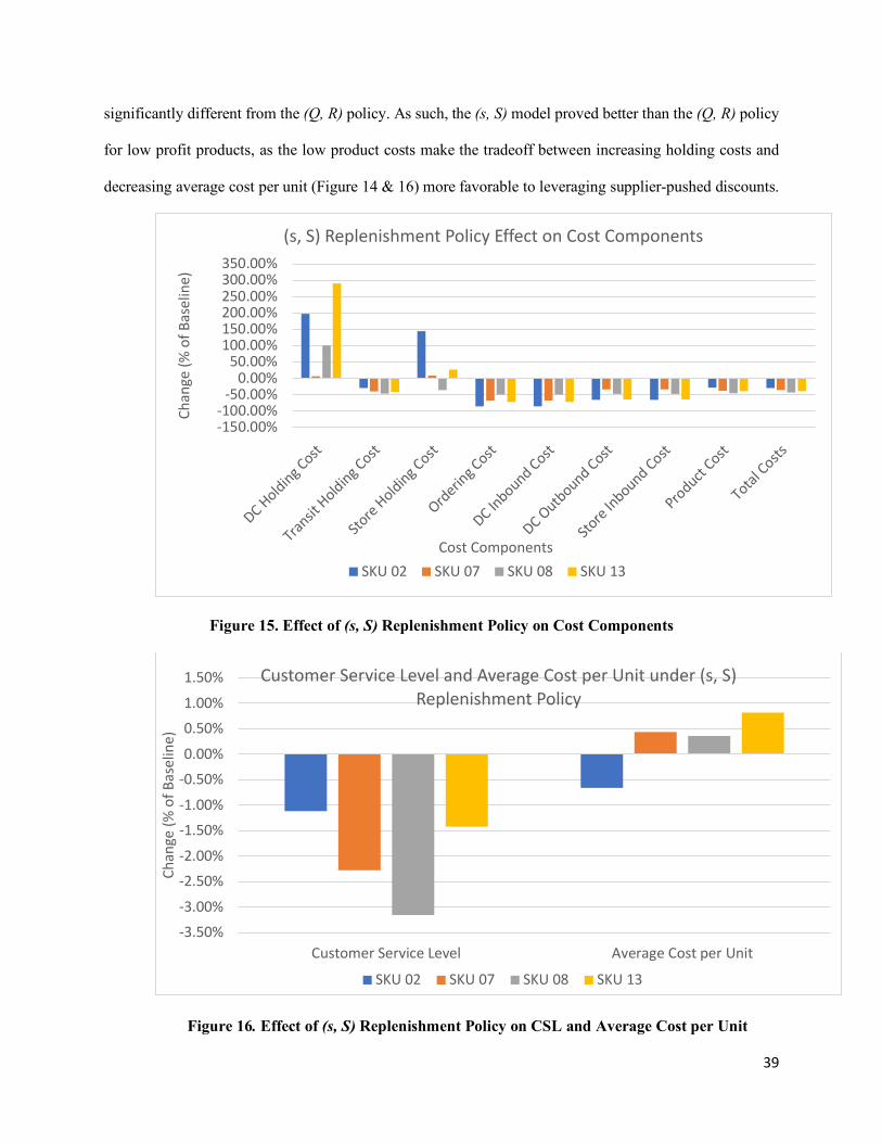
5.3 Continuous review replenishment policy

The (s, S) – (s, S) replenishment model has a better average performance than the (Q, R) model,

with an impact of 37% on average. However, (s, S) policy only performed better in three out of the 16

analyzed SKUs compared to the (Q, R) policy, as effectiveness depends on the SKU characteristics (Figure

17). From the three SKUs, SKU 14 only resulted in 1% more savings in the (s, S) policy over the (Q, R)

policy (Figure 17), and the two remaining SKUs (02 and 13) were both low profit SKUs. For these two

SKUs, the increase in both DC and store holding costs had a lower increase than the (Q, R) policy (Figures

13 and 15). As the (s, S) policy accounts for existing inventory to determine the order size when purchasing

from suppliers and transferring from DC to stores, larger orders than the (Q, R) policy will be preferred.

This is supported in the lower average cost per unit compared to the (Q, R) policy (Figures 14 and

16). These larger orders increased leveraging of supplier-pushed discounts. The CSL for (s, S) was not

-4.00%

-2.00%

0.00%

2.00%

4.00%

6.00%

8.00%

Customer Service Level Average Cost per Unit

Chan

ge (%

of B

asel

ine)

Customer Service Level and Average Cost per Unit under (Q, R) Replenishment Policy


39

significantly different from the (Q, R) policy. As such, the (s, S) model proved better than the (Q, R) policy

for low profit products, as the low product costs make the tradeoff between increasing holding costs and

decreasing average cost per unit (Figure 14 & 16) more favorable to leveraging supplier-pushed discounts.

Figure 15. Effect of (s, S) Replenishment Policy on Cost Components

Figure 16. Effect of (s, S) Replenishment Policy on CSL and Average Cost per Unit

-150.00%-100.00%

-50.00%0.00%

50.00%100.00%150.00%200.00%250.00%300.00%350.00%

DC Holding C

ost

Tran

sit Holding C

ost

Store Holding C

ost

Orderin

g Cost

DC In

bound Cost

DC Outbound Cost

Store In

bound Cost

Product

Cost

Total Costs

Chan

ge (%

of B

asel

ine)

Cost Components

(s, S) Replenishment Policy Effect on Cost Components


-3.50%

-3.00%

-2.50%

-2.00%

-1.50%

-1.00%

-0.50%

0.00%

0.50%

1.00%

1.50%

Customer Service Level Average Cost per Unit

Chan

ge (%

of B

asel

ine)

Customer Service Level and Average Cost per Unit under (s, S) Replenishment Policy


40

Figure 17. Savings per SKU for each inventory model

5.4 Scenario and sensitivity analysis

The scenario analysis tested the fit of the models using both replenishment policies for the DC and

the stores. With these analyses, we determined that having the same model for both the DC and the stores

resulted in a reduction of the total cost, average of 33% for the (Q, R) policy and 37% for the (s, S) policy,

but caused a lower CSL: on average -2.53% for the (Q, R) policy and -2.09% for the (s, S) policy. With the

continuous review policies and short lead times of the sponsor company, the effect of high demand

variability is mitigated and does not seem to affect which policy benefits each SKU more.

High profit SKUs tended to favor the (Q, R) policy, while the (s, S) policy was generally better for

low profit SKUs. Also, we found that using the (s, S) model for both the DC and the stores (Figure 14) has

a better impact in the inventory holding cost while having a similar service level than the baseline for low

profit SKUs. Both policies significantly lowered the inventory total cost in exchange for a small decline in

CSL. On the other hand, this strategy might increase stock-outs to levels that could hurt the company’s

revenue and customer loyalty.

41

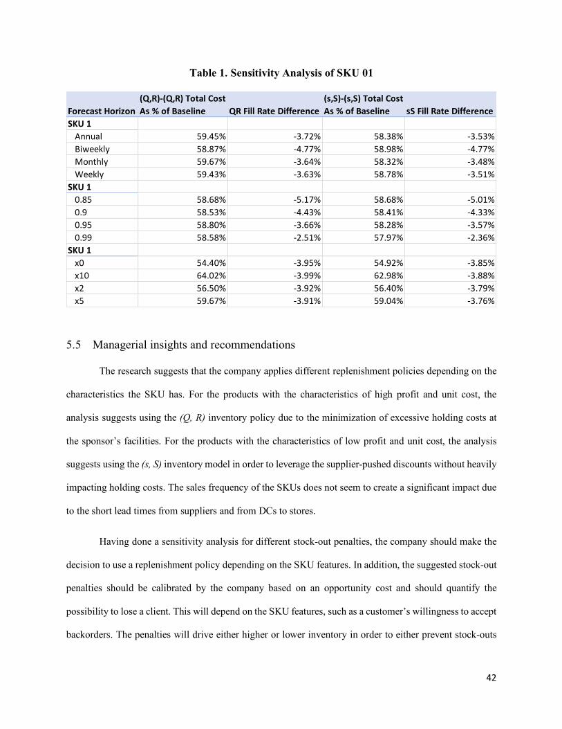
In our sensitivity analyses, we determined which forecasting horizon is the best fit for the couple

of replenishment policies studied in this research by establishing a tradeoff between the total costs and CSL

(see Table 1). In general, the biweekly horizon had the greatest reduction in CSL, while the weekly horizon

is marginally best. Therefore, there is some form of seasonality within the monthly demand which the

sponsor’s forecast technique does not capture in a biweekly horizon. The sales frequency of the SKU also

affects the preferred forecast horizon. For fast-moving SKUs like SKU 01, SKU 08 (See Appendix A), the

replenishment models recommended a lower forecast horizon, given that this type of SKUs experiences

higher stock-outs and the policy carries less inventory, reducing overall holding costs. On the contrary, for

slow-moving SKUs like SKU 12 and SKU 16 (see Appendix A), the replenishment models recommended

a longer forecast horizon in order to reduce the excessive inventory.

We found that the models were sensitive to the stock-out penalty factor used for each SKU. In

general, as the stock-out penalty factor increases, more stock-out costs are incurred with less total savings

compared to the baseline. In addition, the best fit forecast horizon is impacted by the stock-out penalty

factor. A high penalty factor of 10 favors longer forecast horizons, such as annual, while lower penalty

factors of 0, 2 or 5 favor the biweekly forecast horizon. This was consistent with the observed results of the

forecast horizon from the sensitivity analysis. As the biweekly forecast horizon has the greatest reduction

in CSL, experiments with lower stock-out penalty factors placed less emphasis on reducing stock-outs.

Changing the penalty factor from 0 to 10 for high variability SKUs, such as SKU 05 and SKU 10, had a

significant impact in total costs, decreasing the savings of over 15% of baseline on average.

The models also had sensitivity to the defined CSL. Higher CSL drove higher holding costs through

larger order sizes in order to minimize the number of stock-outs, but also leveraged the supplier-pushed

discounts. The CSL sensitivity analysis was also impacted by the stock-out penalty factor. At low stock-

out penalty factors, total costs would increase as CSL increase. However, as the stock-out penalty factor

increased, it was less costly to have higher CSL in order to minimize the stock-outs. Also, we found that

products with high demand variability and low inventory, had a lower CSL compared to the baseline, but

other products were like the baseline.

42

Table 1. Sensitivity Analysis of SKU 01

5.5 Managerial insights and recommendations

The research suggests that the company applies different replenishment policies depending on the

characteristics the SKU has. For the products with the characteristics of high profit and unit cost, the

analysis suggests using the (Q, R) inventory policy due to the minimization of excessive holding costs at

the sponsor’s facilities. For the products with the characteristics of low profit and unit cost, the analysis

suggests using the (s, S) inventory model in order to leverage the supplier-pushed discounts without heavily

impacting holding costs. The sales frequency of the SKUs does not seem to create a significant impact due

to the short lead times from suppliers and from DCs to stores.

Having done a sensitivity analysis for different stock-out penalties, the company should make the

decision to use a replenishment policy depending on the SKU features. In addition, the suggested stock-out

penalties should be calibrated by the company based on an opportunity cost and should quantify the

possibility to lose a client. This will depend on the SKU features, such as a customer’s willingness to accept

backorders. The penalties will drive either higher or lower inventory in order to either prevent stock-outs

Forecast Horizon(Q,R)-(Q,R) Total Cost As % of Baseline QR Fill Rate Difference

(s,S)-(s,S) Total Cost As % of Baseline sS Fill Rate Difference

SKU 1Annual 59.45% -3.72% 58.38% -3.53%Biweekly 58.87% -4.77% 58.98% -4.77%Monthly 59.67% -3.64% 58.32% -3.48%Weekly 59.43% -3.63% 58.78% -3.51%

SKU 10.85 58.68% -5.17% 58.68% -5.01%0.9 58.53% -4.43% 58.41% -4.33%0.95 58.80% -3.66% 58.28% -3.57%0.99 58.58% -2.51% 57.97% -2.36%

SKU 1x0 54.40% -3.95% 54.92% -3.85%x10 64.02% -3.99% 62.98% -3.88%x2 56.50% -3.92% 56.40% -3.79%x5 59.67% -3.91% 59.04% -3.76%

43

or lower inventory holding cost. As such, this paper recommends the sponsor determine different inventory

policies based on the SKU features. With the sponsor’s current forecasting method, an annual forecasting

horizon is suggested for high stock-out penalty SKUs, while a biweekly horizon is suggested for low stock-

out penalty SKUs.

It is important to know that not all SKUs can follow the same replenishment policy to reduce the

total cost. Also, even though the team performed analyses with four different penalties for the 16 SKUs,

not all SKUs have the same stock-out penalty. The company must determine which is the best penalty to

assign to each SKU to determine the best replenishment policy and minimize the impact of either stock-

outs or excess inventory.

44

6 Conclusions and future work

Our analysis was based on the applications of either a (Q, R) replenishment policy and a (s, S)

replenishment policy for both the DC and the stores. The first policy yielded different results such as:

reducing the overall total cost 33% on average, maintaining the CSL similar to the baseline. The second

policy yielded results such as: reducing the overall total cost 37% on average having the higher impact on

the products with high variability having the opportunity to reduce the total cost by 50% while maintaining

a similar fill rate.

The results of the replenishment policies demonstrated the tradeoff between the average unit cost

and overall holding costs of a product. As larger orders were placed to leverage the supplier-pushed

discounts, holding costs increased in response. Eventually, taking advantage of the discounts became

detrimental to the total relevant costs for some SKUs.

Through the sensitivity analysis of stock-out penalty factor, the research demonstrated for that

carrying excess inventory to satisfy demand may be more costly to the sponsor company than having a

stock-out event occur. As such, SKUs need to be examined for the probability a customer will accept a

backorder and the risk of losing a customer’s future lost sales to a competitor.

This paper recommends using the (Q, R) replenishment policy for SKUs with the high profit and

using the (s, S) replenishment policy for SKUs with low profit. Neither the volume of demand or variability

of demand made significant impacts in this experiment due to the short lead times experience by the sponsor

company.

Having determined the benefits and limitations of both models in the scenarios tested, the capstone

recommends further analysis on the applications of other scenarios. The scenario that the team is

recommending to further analyze is using a different policy for the DC and the stores and understand the

benefits and complexities these may bring. Further scenarios could be tested with a configuration of having

the DC with one of the policies and each SKU/Store configuration having a different policy depending on

the characteristics of demand of each SKU/Store. Also, the team recommend understanding the demand

45

and the customers that each product and store since stock-out penalties may vary depending on the type of

customer the store/SKU is serving.

Also, it is recommended to calculate the impact of the DC stock-outs due to the relation between

stock-outs from the DC and from the stores. These were not directly addressed in the research but, further

research is suggested to capture an incremental penalty for stock-outs at the DC to be captured in the total

relevant cost at the DC. These mentioned stock-out may come from various factors such as suppliers item

fill rate lower than 100% or an ordered quantity lower than needed.

The implementation of the different replenishment policies analyzed has a high potential of costs

reduction. While these policies may have an impact on the CSL, the overall savings can far exceed the

penalties. From the research we concluded that the application of the analyzed policies can bring an average

33% saving of the total relevant cost.

46

References

Alicke, K., Ebel, T., Schrader, U., & Shah, K. (2014). Finding Opportunity in Uncertainty: A New Paradigm for Pharmaceutical Supply Chains. Available at: https://www.mckinsey.com/~/media/mckinsey/dotcom/client_service/pharma%20and%20medical%20products/pmp%20new/pdfs/finding_opportunity_in_uncertainty-introductory_chapter.ashx

Anand, S. & Chadha, S. (2019). Out-of-stocks are more costly than losing a sale — but there's a fix Available at: https://www.supplychaindive.com/news/reduce-retail-out-of-stock-AT-Kearney/545439/

Cárdenas-Barrón, L. E., & Sana, S. S. (2015). Multi-item EOQ inventory model in a two-layer supply chain while demand varies with promotional effort. Applied Mathematical Modelling, 39(21), 6725-6737.

Cheng, S. H., & Whittemore, G. J. (2008). An engineering approach to improving hospital supply chains. (Unpublished master's thesis). Massachusetts of Institute of Technology, Cambridge, MA.

CVS Health Corporation. (2019). 2017 Annual Report. Retrieved from http://www.investors.cvshealth.com Evaluate LTD. (2017) World Preview 2017 Outlook to 2022. Retrieved March, 2019 from

http://info.evaluategroup.com/rs/607-YGS-364/images/WP17.pdf Ghosh, S., Khanra, S., & Chaudhuri, K. (2011). Optimal price and lot size determination for a perishable

product under conditions of finite production, partial backordering and lost sale. Applied Mathematics and Computation, 217(13), 6047-6053.

Guerrero, W., Yeung, T., & Guéret, C. (2013). Joint-optimization of inventory policies on a multi-product multi-echelon pharmaceutical system with batching and ordering constraints. European Journal of Operational Research, 231(1), 98-108.

Güder, F., Zydiak, J., Chaudhry, S. (1994). Capacitated Multiple Item Ordering with Incremental Quantity Discounts. The Journal of the Operational Research Society. 45(10):1197-1205

Industria de Diseño Textil S.A. (2018). 2018 Annual Report. Retrieved from http://www.inditex.com/investors/investor-relations/annual-reports

Keeling, D., Lösch, M., & Schrader, U. (2010). Outlook on pharma operations. Available at: https://www.mckinsey.com/~/media/mckinsey/dotcom/client_service/operations/pdfs/outlook_on_pharma_operations.ashx

Kelle, P., Woosley, J., & Schneider, H. (2012). Pharmaceutical supply chain specifics and inventory solutions for a hospital case. Operations Research for Health Care, 1(2-3), 54-63.

Knuth, K.H., Castle, J.P., & Wheeler, K.R. (2006). Identifying excessively rounded or truncated data. Proceedings of the 17th meeting of the International Association for Statistical Computing – Europen Regional Section: Computational Statistics (COMPSTAT 2006), Rome, Italy, August 2006.

Nematollahi, M., Hosseini-Motlagh, S., & Heydari, J. (2017). Economic and social collaborative decision-making on visit interval and service level in a two-echelon pharmaceutical supply chain. Journal of Cleaner Production, 142, 3956-3969.

Nicholson, L., Vakharia, A. J., & Erenguc, S. S. (2004). Outsourcing inventory management decisions in healthcare: Models and application. European Journal of Operational Research, 154(1), 271-290.

O’Donnell, T.O., Maguire, L. McIvor, R., & Humphreys, P. (2007). Reducing the Bullwhip Effect when Facing Sales Promotions: A Genetic Algorithm Approach. Available at: https://pdfs.semanticscholar.org/6ecf/9a16dc781ecd5ee8b06ee26d92db958add56.pdf

Saedi, S., Kundakcioglu, O. E., & Henry, A. C. (2016). Mitigating the impact of drug shortages for a healthcare facility: An inventory management approach. European Journal of Operational Research, 251(1), 107-123.

Sanchez-Ruiz, L., Blanco, B., & Kyguoliene, A. (2018). A Theoretical Overview of the Stock-out Problem in Retail: from Causes to Consequences. Management of Organizations: Systematic Research, 79(1), 103-116.

47

Saracoglu, I., Topaloglu, S., & Keskinturk, T. (2014). A genetic algorithm approach for multi-product multi-period continuous review inventory models. Expert Systems with Applications, 41(18), 8189-8202.

Shteren, H., & Avrahami, A. (2017). The Value of Inventory Accuracy in Supply Chain Management - Case Study of the Yedioth Communication Press. Journal of Theoretical & Applied Electronic Commerce Research, Volume 12(2), 71-86.

Simatupang, T.M., & Sridharan, R. (2005). An integrative framework for supply chain collaboration. The International Journal of Logistics Management, 16 (2), 257-274.

Target Corporation. (2019). 2018 Annual Report. Retrieved from http://www.investors.target.com Tompkins International. (2018) Inventory Management Survey Results. Available at:

https://www.supplychainconsortium.com/Report/GetReport/Inventory-Management-Survey-Results

The Plunkett Research Group. (2019). Health Care Trends. Available at: https://www.plunkettresearch.com/industries/health-care-medical-market-research/

Uthayakumar, R., & Priyan, S. (2013). Pharmaceutical supply chain and inventory management strategies: Optimization for a pharmaceutical company and a hospital. Operations Research for Health Care, 2(3), 52-64.

Vries, J. D. (2011). The shaping of inventory systems in health services: A stakeholder analysis. International Journal of Production Economics, 133(1), 60-69.

Vrata, A. (2012). Vendor Managed Inventory: Providing Visibility Across the Pharma R&D Supply Chain. Available at: https://www.cognizant.com/industries-resources/life_sciences/Vendor-Managed-Inventory-Providing-Visibility-Across-the-Pharma-RandD-Supply-Chain.pdf

Wadhwa, S., Bibhushan, & Chan, F. T. (2009). Inventory performance of some supply chain inventory policies under impulse demands. International Journal of Production Research, 47(12), 3307-3332.

Walgreens Boots Alliance, Inc. (2019). 2018 Annual Report. Retrieved from http://www.investor.walgreensbootsalliance.com

Walmart Inc. (2019). 2018 Annual Report. Retrieved from http://www.stock.walmart.com Wollenhaupt, G. (2018). Managing inventory: What retail can learn from pharma. Available at:

https://www.supplychaindive.com/news/retail-pharmaceutical-supply-chain-inventory-spotlight/539696/

48

APPENDIX A Sensitivity Analysis Using Four Different Forecast Horizons

Forecast Horizon(Q,R)-(Q,R) Total Cost As % of Baseline QR Fill Rate Difference

(s,S)-(s,S) Total Cost As % of Baseline sS Fill Rate Difference



SKU 3Annual 78.49% -2.28% 81.04% -0.49%Biweekly 78.32% -2.44% 81.76% -1.07%Monthly 79.85% -2.07% 82.67% -0.57%Weekly 86.98% 0.50% 89.63% 0.92%

SKU 4Annual 77.76% -0.09% 79.28% 0.20%Biweekly 75.26% -3.71% 79.45% -2.36%Monthly 78.31% -0.15% 77.94% 0.20%Weekly 79.58% 0.08% 79.64% 0.57%








SKU 12Annual 70.54% -1.18% 71.41% 0.69%Biweekly 81.45% -0.83% 83.06% 0.74%Monthly 78.47% -0.83% 78.83% 0.78%Weekly 89.61% -0.34% 93.13% 1.46%




SKU 16Annual 79.87% 0.27% 82.03% 4.81%Biweekly 88.50% 0.93% 86.25% 4.41%Monthly 82.48% 0.72% 80.80% 5.01%Weekly 102.02% 1.26% 94.20% 4.70%

49

APPENDIX B Sensitivity Analysis Using Four Different Cycle Service Levels

Cycle Service Level QR Average Cost QR Fill Rate Difference sS Average Cost sS Fill Rate DifferenceSKU 10.85 58.68% -5.17% 58.68% -5.01%0.9 58.53% -4.43% 58.41% -4.33%0.95 58.80% -3.66% 58.28% -3.57%0.99 58.58% -2.51% 57.97% -2.36%

SKU 20.85 72.67% -1.76% 64.46% -1.36%0.9 72.36% -1.73% 64.18% -1.32%0.95 72.00% -1.63% 64.04% -1.33%0.99 71.21% -1.15% 67.55% -0.45%

SKU 30.85 83.07% -2.40% 85.91% -1.23%0.9 82.90% -2.35% 84.63% -1.14%0.95 82.04% -2.04% 86.90% -0.88%0.99 86.49% 0.49% 87.95% 2.03%

SKU 40.85 81.08% -2.37% 85.08% -2.03%0.9 80.28% -1.76% 83.06% -1.27%0.95 79.26% -0.75% 83.89% 0.13%0.99 82.66% 1.01% 82.66% 1.79%

SKU 50.85 75.09% -6.72% 78.37% -7.43%0.9 75.12% -5.89% 77.60% -6.77%0.95 74.69% -4.14% 76.98% -5.63%0.99 74.60% -3.22% 75.36% -3.98%

SKU 60.85 54.12% -3.37% 54.20% -3.16%0.9 53.73% -2.91% 54.06% -2.58%0.95 53.31% -2.38% 54.25% -2.29%0.99 54.88% -1.40% 54.65% -1.24%

SKU 70.85 61.56% -2.99% 62.88% -2.66%0.9 61.18% -2.70% 62.50% -2.17%0.95 61.09% -2.77% 62.21% -2.26%0.99 60.83% -2.72% 61.92% -2.02%

SKU 80.85 55.56% -4.10% 57.21% -4.15%0.9 55.04% -3.69% 56.44% -3.66%0.95 55.73% -2.81% 56.49% -3.08%0.99 55.57% -1.78% 56.14% -1.73%

SKU 9 0.85 68.60% -3.59% 71.60% -3.78%0.9 67.52% -2.96% 71.08% -3.16%0.95 69.54% -1.96% 70.89% -2.30%0.99 69.16% -1.05% 69.21% -0.90%

SKU 100.85 59.62% -8.32% 60.08% -8.98%0.9 59.25% -8.00% 59.65% -8.88%0.95 60.07% -7.38% 60.30% -8.39%0.99 59.63% -4.08% 60.46% -6.04%

SKU 110.85 64.51% -1.19% 63.33% -1.09%0.9 64.52% -1.07% 64.74% -0.96%0.95 64.17% -0.91% 66.88% -0.68%0.99 65.83% -0.48% 66.02% -0.11%

SKU 120.85 74.05% -1.19% 74.70% 0.68%0.9 71.62% -0.95% 73.29% 0.69%0.95 70.26% -1.04% 72.29% 0.74%0.99 71.10% 0.01% 69.70% 1.55%

SKU 130.85 62.08% -1.88% 59.20% -1.98%0.9 61.72% -1.57% 59.38% -1.79%0.95 61.51% -1.24% 59.02% -1.36%0.99 60.96% -0.63% 59.29% -0.57%

SKU 140.85 64.09% -4.75% 62.51% -4.59%0.9 63.65% -3.97% 62.33% -3.86%0.95 63.95% -3.08% 61.88% -3.01%0.99 62.91% -2.03% 61.59% -1.87%

SKU 150.85 60.60% -4.50% 62.43% -4.02%0.9 60.17% -4.64% 61.60% -4.64%0.95 59.63% -4.27% 61.64% -3.42%0.99 59.36% -2.61% 62.42% -2.69%

SKU 160.85 79.28% 0.83% 82.04% 4.89%0.9 84.51% 0.68% 80.77% 4.66%0.95 81.08% 0.78% 80.52% 4.70%0.99 82.75% 0.89% 82.28% 4.68%

50

APPENDIX C Sensitivity Analysis Using Four Different Stock-Out Penalty Factors

Stock-Out Penalty QR Average Cost QR Fill Rate Difference sS Average Cost sS Fill Rate DifferenceSKU 1x0 54.40% -3.95% 54.92% -3.85%x10 64.02% -3.99% 62.98% -3.88%x2 56.50% -3.92% 56.40% -3.79%x5 59.67% -3.91% 59.04% -3.76%

SKU 2x0 69.64% -1.52% 62.72% -1.09%x10 75.37% -1.60% 68.08% -1.19%x2 70.75% -1.57% 63.90% -1.10%x5 72.49% -1.58% 65.53% -1.07%

SKU 3x0 72.05% -2.06% 76.73% -0.69%x10 97.56% -1.26% 98.08% -0.25%x2 78.17% -1.59% 81.56% -0.17%x5 86.73% -1.38% 89.02% -0.11%

SKU 4x0 69.52% -0.98% 74.34% -0.33%x10 94.64% -0.94% 95.08% -0.28%x2 75.36% -1.00% 79.86% -0.40%x5 83.76% -0.95% 85.41% -0.38%

SKU 5x0 65.29% -5.00% 67.63% -6.07%x10 86.67% -4.97% 89.34% -5.76%x2 70.32% -5.01% 72.12% -5.98%x5 77.20% -4.98% 79.22% -6.01%

SKU 6x0 51.54% -2.53% 52.04% -2.33%x10 57.36% -2.52% 56.92% -2.35%x2 52.70% -2.53% 53.03% -2.31%x5 54.44% -2.48% 55.16% -2.28%

SKU 7x0 57.80% -3.25% 59.04% -2.73%x10 64.60% -2.37% 65.70% -2.03%x2 60.26% -2.91% 61.35% -2.24%x5 62.00% -2.66% 63.41% -2.10%

SKU 8x0 52.18% -3.14% 54.13% -3.09%x10 59.68% -3.03% 60.21% -3.14%x2 53.82% -3.11% 55.10% -3.22%x5 56.20% -3.11% 56.85% -3.17%

SKU 9x0 64.21% -2.39% 66.24% -2.65%x10 74.56% -2.41% 76.17% -2.41%x2 66.40% -2.38% 68.41% -2.47%x5 69.66% -2.37% 71.96% -2.61%

SKU 10x0 52.37% -8.36% 52.55% -9.73%x10 67.16% -5.64% 68.35% -6.66%x2 57.12% -7.24% 57.29% -8.34%x5 61.92% -6.54% 62.30% -7.56%

SKU 11x0 64.55% -0.91% 65.08% -0.75%x10 66.57% -0.90% 66.39% -0.70%x2 63.35% -0.93% 64.83% -0.72%x5 64.55% -0.91% 64.66% -0.67%

SKU 12x0 68.58% -0.80% 70.67% 1.07%x10 75.60% -0.69% 75.65% 0.73%x2 69.67% -0.83% 71.21% 1.00%x5 73.16% -0.85% 72.45% 0.87%

SKU 13x0 60.13% -1.34% 57.55% -1.42%x10 63.53% -1.35% 61.52% -1.46%x2 60.81% -1.33% 58.39% -1.43%x5 61.79% -1.29% 59.42% -1.40%

SKU 14x0 59.88% -3.50% 58.84% -3.35%x10 68.46% -3.48% 66.14% -3.34%x2 61.68% -3.44% 60.46% -3.34%x5 64.57% -3.42% 62.86% -3.29%

SKU 15x0 54.85% -4.53% 57.31% -4.66%x10 66.18% -3.36% 67.28% -3.13%x2 57.98% -4.23% 60.75% -3.69%x5 60.75% -3.91% 62.76% -3.31%

SKU 16x0 76.83% 0.72% 79.30% 4.60%x10 87.78% 0.83% 82.65% 4.81%x2 80.52% 0.80% 81.50% 4.83%x5 82.48% 0.83% 82.18% 4.70%

replenishment policies for retail pharmacies in emerging

Documents