report bre e302 040707 - strath · introduction ... esru consultancy 4 july 2007 report page 3...
TRANSCRIPT
ESRU
report
Energy Systems Research Unit Dept. of Mechanical Engineering James Weir Building 75 Montrose Street Glasgow G1 1XJ
Email: [email protected] Tel: +44 (0)141 548 5765 Fax: +44 (0)141 552 5105 http://www.esru.strath.ac.uk
Development of a Methodology for the Evaluation of Domestic Heating Controls Phase 2 of a DEFRA Market Transformation Programme project, carried out under contract to BRE Environment Final Report – (phase 2) Jeremy Cockroft, Aizaz Samuel, Paul Tuohy Energy Systems Research Unit 4th July 2007
Contents Executive Summary ......................................................................................................1 Introduction....................................................................................................................2 Modelling Overview .......................................................................................................2 Modelling Details ...........................................................................................................4
Houses.......................................................................................................................4 Boilers........................................................................................................................5 Domestic Hot Water...................................................................................................8 Heating systems ........................................................................................................9 Controls ...................................................................................................................10
On/off room thermostat ........................................................................................10 Electronic PI thermostat .......................................................................................11 Weather compensated control .............................................................................12 Overall controls integration...................................................................................12
Modelling of House, System and Control Interactions.................................................16 Graphs of Control Performance of Selected Combinations .....................................16 Histograms of Energy Consumption for Selected Combinations .............................25
Controls Evaluation Model...........................................................................................34 SAP and BREDEM development ................................................................................37
The influence of controls on SAP / BREDEM calculations.......................................37 1-A. Hot water: .....................................................................................................37 1-B. Space heating:..............................................................................................37 1-B-1. Efficiencies: ...............................................................................................37 1-B-2. Heating type and responsiveness (living room temperature):....................37 1-B-3. Further Controls details (living room temp adjust, non living temperature):.............................................................................................................................38
SAP calculations......................................................................................................38 Recommendations for developing SAP ...................................................................40
Conclusion...................................................................................................................41 Appendix 1 – Casual Gains.........................................................................................42 Appendix 2 - Plant Parameters....................................................................................44 List of Figures Figure 1 – boiler model schematic and logic. 5 Figure 2 – Condensing gas boiler efficiency curves. 6 Figure 3 – Non condensing gas boiler efficiency curves. 7 Figure 4 - Condensing oil boiler efficiency curves (flue gas temperature 5K above return water temperature. 7 Figure 5 – Combi boiler in domestic hot water mode. 8 Figure 6 – baseline control system 10 Figure 7 – Thermostat model schematic 11 Figure 8 – Electronic PI thermostat schematic 11 Figure 9 – Weather compensated control schematic 12 Figure 10 - Assimilation of zone / dhw control actions into boiler control model. 12 Figure 11 - Zone temperatures for Baseline case (House3, plant2, control2) 17 Figure 12 – System temperatures for Baseline case (House3, plant2, control2) 18 Figure 13 – Comparison of zone temperatures for five house types, thermostat control. 19 Figure 14 – Comparison radiator temperatures for five house types, thermostat control. 19
Figure 15 – Comparison of modulating condensing and on/off non-condensing boilers. 20 Figure 16 – Comparison of storage and combi DHW systems 20 Figure 17 – Comparison of OTC and room thermostat control systems 21 Figure 18 – Comparison of underfloor system with OTC control and radiator system with thermostat control. 22 Figure 19 – Comparison living and non-living resultant temperatures with TRVs and no TRVs in non-living area. 22 Figure 20 – Two zone thermostat control 23 Figure 21 – Comparison of thermostat and PI room control. 23 Figure 22 – Comparison of gas and oil boilers 24 Figure 23 – Seasonal and annual energy consumption for five house types. 25 Figure 24 – Comparison of condensing and non-condensing boilers. 26 Figure 25 – Comparison of regular and combi boilers 27 Figure 26 – Comparison of room thermostat and OTC control with radiators. 28 Figure 27 – Comparison of radiator (thermostat) and underfloor heating (OTC) systems 29 Figure 28 – Comparison of non-living zone without and with TRVs. 30 Figure 29- Comparison of single and two zone thermostat control 31 Figure 30 – Comparison of on/off thermostat with PI modulating room control. 32 Figure 31 – Comparison of gas and oil boilers 33 Figure 32 - ADEPT Display Centre 34 Figure 33 – ADEPT Energy Totaliser 35 Figure 34 – ADEPT interface for ESP-r 36 Figure 35 – SAP 2005 Environmental Index scores for a range of house types. 39 Figure 36 – SAP Environmental Index scores for the baseline house, for a range of system and control types. 39 List of Tables Table 1 - House, boiler, heating circuit, and control type options 3 Table 2 – Summary data for house types 4 Table 3 - Boiler efficiency curve fit polynomial coefficients 8 Table 4 – Hot water draw-off schedule 9 Table 5 - User adjustable parameters 13 Table 6 – Combinations of house, boiler / heating circuit and control types for analysis 16 Table 7 - Analysis days for annual energy consumption. 25 Table 8 - A selection of the metrics behind Figure 35. 40 Table 9 - A selection of metrics behind Figure 36. 40
ESRU Consultancy 4 July 2007 Report Page 1
Executive Summary The objective of this project is to produce a controls evaluation methodology based on computer modelling of domestic housing and heating systems. The results from this project will allow the Government’s Standard Assessment Procedure (SAP) for home energy rating to be further developed so that energy saving benefits of advanced controls may be recognised within the procedure, particularly in relation to maximising the benefits of condensing boilers.
The evaluation methodology takes into account typical UK housing characteristics, climate, occupancy patterns, boiler, and heating system types using the modelling tool ESP-r. Five house types, five heating system types and five control system types were agreed for analysis. House types broadly reflect the range of housing stock to which SAP will be applied. Heating system types include non-condensing and condensing boilers, regular and combi boilers, gas and oil boilers, and both radiator and underfloor heat emitters. Controls range from a basic system with a single room thermostat, through to a two-zone system with two independent thermostats. Electronic controllers are also represented, both room temperature and outdoor temperature based. The results of a selection of simulations of twenty combinations of house, system and control scheme demonstrate how choice of house size and type, burner / room control regulation mode, system operating flow and return temperature, weather compensation and choice of zoning strategy affect the zone and system temperatures, system performance, and annual energy use.
Annual heating energy consumption shows a high degree of sensitivity to factors other than inherent system efficiency. In particular, overnight rate of cool down, and fixed timer settings interact with construction and system thermal mass to affect the results in unanticipated ways.
An interface to ESP-r called ADEPT (Advanced Domestic Energy Prediction Tool) facilitates set up of any desired combinations of the defined house, system and control schemes, producing standardised outputs demonstrating control behaviour and energy use.
Suggestions for SAP / BREDEM development, using the results from the evaluation methodology are proposed.
ESRU Consultancy 4 July 2007 Report Page 2
Introduction In April 2005 the Building Regulations for England and Wales were amended such that, in most cases, new and replacement gas and oil boilers require to be condensing. This has dramatically transformed the market for boilers, as it sets new standards of efficiency that are approaching their practical limit. Consequently, attention has now shifted to improving heating system controls so that these efficiency benefits may be more effectively achieved in practice.
At present there is no authoritative basis for the evaluation of the energy benefits of advanced domestic heating controls, and energy saving claims are difficult to substantiate or refute. The objective of this project is to produce a controls evaluation methodology based on computer modelling of domestic housing and heating systems. The results from this project will allow the Government’s Standard Assessment Procedure (SAP) for home energy rating to be further developed so that energy saving benefits of advanced controls may be recognised within the procedure.
The evaluation methodology takes into account typical UK housing characteristics, climate, occupancy patterns, boiler, and heating system types. The modelling tool used throughout this project is ESP-r. ESP-r is a world renowned integrated transient energy modelling tool for the simulation of the thermal, visual and acoustic performance of buildings and the assessment of energy use. In undertaking its assessments, the system is equipped to model heat, air, moisture and electrical power flows at user determined resolution. ESP-r has been validated through International Energy Agency comparison projects. It is at work in some of the world’s largest commercial, government and academic institutions.
Modelling Overview ESP-r models the energy and fluid flows within combined building and plant systems when constrained to conform to control action. One or more zones within a building are defined in terms of geometry, construction and usage profiles. These zones are then inter-linked to form a building. Building fabric elements are defined in terms of multi-layer constructions, using material data that defines thermophysical properties of conductivity, density, specific heat, solar absorptivity and emissivity for each homogenous element. Optical properties are defined for transparent elements. Internal view factors are calculated in order to improve modelling of longwave radiation exchanges. Internal and external convection coefficients are calculated at run time, along with casual convective and radiative gains according to the occupancy schedule. Plant models consist of thermally dynamic elements, such as heat generators and emitters, thermostat sensors and distribution pipework, and control logic elements that respond to building and plant variables by acting on actuators to control flow, or to inject heat, for example. Simulation proceeds at discrete time steps, in this case one minute for the building and five seconds for the plant and controls, in order that short time constant dynamics associated with plant and controls are accurately replicated. Five house types, five heating system types and five control system types were agreed for analysis, and are summarised in Table 1.
ESRU Consultancy 4 July 2007 Report Page 3
Number House Type Boiler and Heat Circuit
Type Control Type
1 Detached solid wall single glazed pre-1918 100mm loft insulation.
Gas, non-condensing, regular boiler, non-modulating burner, radiators
Living room mechanical thermostat, no TRVs
2 Semi-detached unisulated cavity wall, single glazed 1939-59 100mm loft insulation.
Gas, condensing, regular boiler, modulating burner, radiators
Living room mechanical thermostat, TRVs in other rooms
3 Semi-detached, EEC stock average, 100mm loft insulation, filled cavity, 100mm loft insulation
Gas, condensing, combi boiler, modulating burner, radiators
Living room and Non-living zone mechanical thermostats
4 Semi-detached timber frame 1990 – 1999, double glazed 100mm loft insulation.
Oil, condensing, regular boiler, non-modulating burner, radiators
Weather (outside temperature) compensation, modulating supply water set point. Living room temperature compensation. TRVs in other rooms.
5 mid-terrace 2006 (pt L regs.) filled cavity 270mm loft insulation
Gas, condensing, regular boiler, modulating burner, heavy underfloor system in living room, radiators in other rooms.
Living room sensor, modulating supply water set point. TRVs in other rooms.
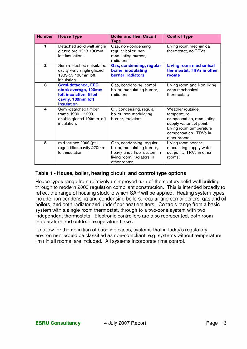
Table 1 - House, boiler, heating circuit, and control type options
House types range from relatively unimproved turn-of-the-century solid wall building through to modern 2006 regulation compliant construction. This is intended broadly to reflect the range of housing stock to which SAP will be applied. Heating system types include non-condensing and condensing boilers, regular and combi boilers, gas and oil boilers, and both radiator and underfloor heat emitters. Controls range from a basic system with a single room thermostat, through to a two-zone system with two independent thermostats. Electronic controllers are also represented, both room temperature and outdoor temperature based.
To allow for the definition of baseline cases, systems that in today’s regulatory environment would be classified as non-compliant, e.g. systems without temperature limit in all rooms, are included. All systems incorporate time control.
ESRU Consultancy 4 July 2007 Report Page 4
Modelling Details
Houses
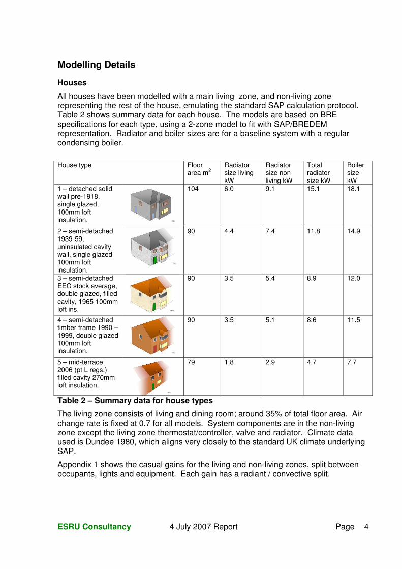
All houses have been modelled with a main living zone, and non-living zone representing the rest of the house, emulating the standard SAP calculation protocol. Table 2 shows summary data for each house. The models are based on BRE specifications for each type, using a 2-zone model to fit with SAP/BREDEM representation. Radiator and boiler sizes are for a baseline system with a regular condensing boiler.
House type Floor
area m2 Radiator size living kW
Radiator size non-living kW
Total radiator size kW
Boiler size kW
1 – detached solid wall pre-1918, single glazed, 100mm loft insulation.
104 6.0 9.1 15.1 18.1
2 – semi-detached 1939-59, uninsulated cavity wall, single glazed 100mm loft insulation.
90 4.4 7.4 11.8 14.9
3 – semi-detached EEC stock average, double glazed, filled cavity, 1965 100mm loft ins.
90 3.5 5.4 8.9 12.0
4 – semi-detached timber frame 1990 – 1999, double glazed 100mm loft insulation.
90 3.5 5.1 8.6 11.5
5 – mid-terrace 2006 (pt L regs.) filled cavity 270mm loft insulation.
79 1.8 2.9 4.7 7.7
Table 2 – Summary data for house types
The living zone consists of living and dining room; around 35% of total floor area. Air change rate is fixed at 0.7 for all models. System components are in the non-living zone except the living zone thermostat/controller, valve and radiator. Climate data used is Dundee 1980, which aligns very closely to the standard UK climate underlying SAP.
Appendix 1 shows the casual gains for the living and non-living zones, split between occupants, lights and equipment. Each gain has a radiant / convective split.
ESRU Consultancy 4 July 2007 Report Page 5
Boilers
A boiler is modelled as a “black box”, in other words, we do not model the actual combustion process explicitly. This would require some detail of individual boiler construction, whereas we are seeking a more general approach.
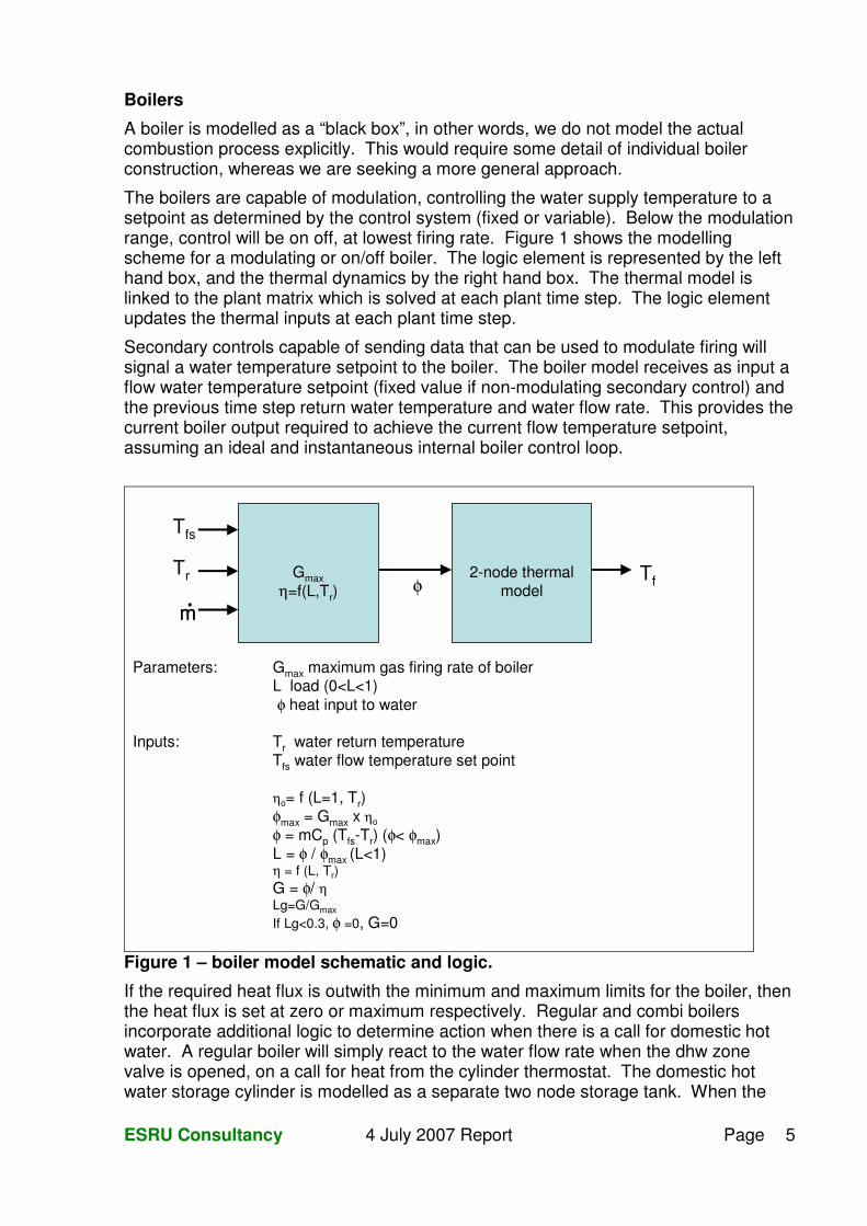
The boilers are capable of modulation, controlling the water supply temperature to a setpoint as determined by the control system (fixed or variable). Below the modulation range, control will be on off, at lowest firing rate. Figure 1 shows the modelling scheme for a modulating or on/off boiler. The logic element is represented by the left hand box, and the thermal dynamics by the right hand box. The thermal model is linked to the plant matrix which is solved at each plant time step. The logic element updates the thermal inputs at each plant time step.
Secondary controls capable of sending data that can be used to modulate firing will signal a water temperature setpoint to the boiler. The boiler model receives as input a flow water temperature setpoint (fixed value if non-modulating secondary control) and the previous time step return water temperature and water flow rate. This provides the current boiler output required to achieve the current flow temperature setpoint, assuming an ideal and instantaneous internal boiler control loop.
Parameters: Gmax maximum gas firing rate of boilerL load (0<L<1)φ heat input to water
Inputs: Tr water return temperatureTfs water flow temperature set point
ηo= f (L=1, Tr)φmax = Gmax x ηo
φ = mCp (Tfs-Tr) (φ< φmax)L = φ / φmax (L<1)η = f (L, Tr)G = φ/ ηLg=G/Gmax
If Lg<0.3, φ =0, G=0
Gmaxη=f(L,Tr)
Tfs
φTr
m.
m.
2-node thermalmodel
Tf
Figure 1 – boiler model schematic and logic.
If the required heat flux is outwith the minimum and maximum limits for the boiler, then the heat flux is set at zero or maximum respectively. Regular and combi boilers incorporate additional logic to determine action when there is a call for domestic hot water. A regular boiler will simply react to the water flow rate when the dhw zone valve is opened, on a call for heat from the cylinder thermostat. The domestic hot water storage cylinder is modelled as a separate two node storage tank. When the
ESRU Consultancy 4 July 2007 Report Page 6
domestic hot water call is satisfied (hot water temperature rises to the upper thermostat limit) the zone valve is closed.
A combi boiler will switch to DHW service mode. In this case, the heat flux to the DHW, supplied via an internal fast response heat exchanger is known. The heat exchanger is modelled in a similar fashion to the storage cylinder, but with low thermal mass. The known heat flux to be supplied by the boiler enables the flow and return temperatures to be determined dynamically, and the boiler will modulate as necessary, mimicking the behaviour of a combi boiler maintaining a fixed dhw supply temperature.
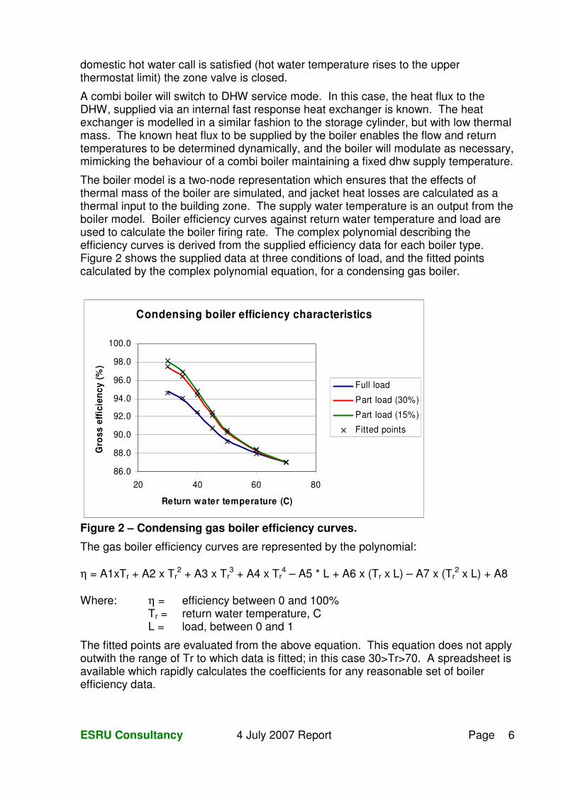
The boiler model is a two-node representation which ensures that the effects of thermal mass of the boiler are simulated, and jacket heat losses are calculated as a thermal input to the building zone. The supply water temperature is an output from the boiler model. Boiler efficiency curves against return water temperature and load are used to calculate the boiler firing rate. The complex polynomial describing the efficiency curves is derived from the supplied efficiency data for each boiler type. Figure 2 shows the supplied data at three conditions of load, and the fitted points calculated by the complex polynomial equation, for a condensing gas boiler.
Condensing boiler efficiency characteristics
86.0
88.0
90.0
92.0
94.0
96.0
98.0
100.0
20 40 60 80
Return water temperature (C)
Gro
ss e
ffici
ency
(%)
Full load
Part load (30%)
Part load (15%)
Fitted points
Figure 2 – Condensing gas boiler efficiency curves.
The gas boiler efficiency curves are represented by the polynomial: η = A1xTr + A2 x Tr
2 + A3 x Tr3 + A4 x Tr
4 – A5 * L + A6 x (Tr x L) – A7 x (Tr2 x L) + A8
Where: η = efficiency between 0 and 100% Tr = return water temperature, C L = load, between 0 and 1
The fitted points are evaluated from the above equation. This equation does not apply outwith the range of Tr to which data is fitted; in this case 30>Tr>70. A spreadsheet is available which rapidly calculates the coefficients for any reasonable set of boiler efficiency data.
ESRU Consultancy 4 July 2007 Report Page 7
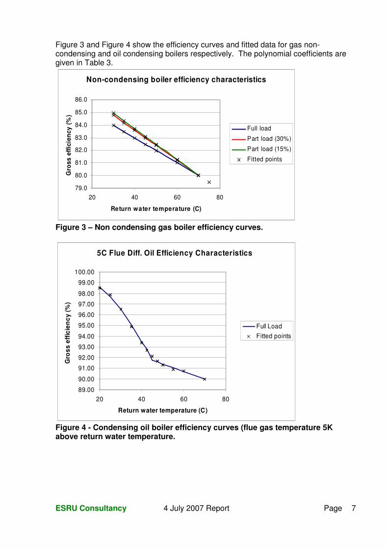
Figure 3 and Figure 4 show the efficiency curves and fitted data for gas non-condensing and oil condensing boilers respectively. The polynomial coefficients are given in Table 3.
Non-condensing boiler efficiency characteristics
79.0
80.0
81.0
82.0
83.0
84.0
85.0
86.0
20 40 60 80
Return water temperature (C)
Gro
ss e
ffici
ency
(%)
Full load
Part load (30%)
Part load (15%)
Fitted points
Figure 3 – Non condensing gas boiler efficiency curves.
5C Flue Diff. Oil Efficiency Characteristics
89.00
90.00
91.00
92.00
93.00
94.00
95.00
96.00
97.00
98.00
99.00
100.00
20 40 60 80
Return water temperature (C)
Gro
ss e
ffici
ency
(%)
Full LoadFitted points
Figure 4 - Condensing oil boiler efficiency curves (flue gas temperature 5K above return water temperature.
ESRU Consultancy 4 July 2007 Report Page 8
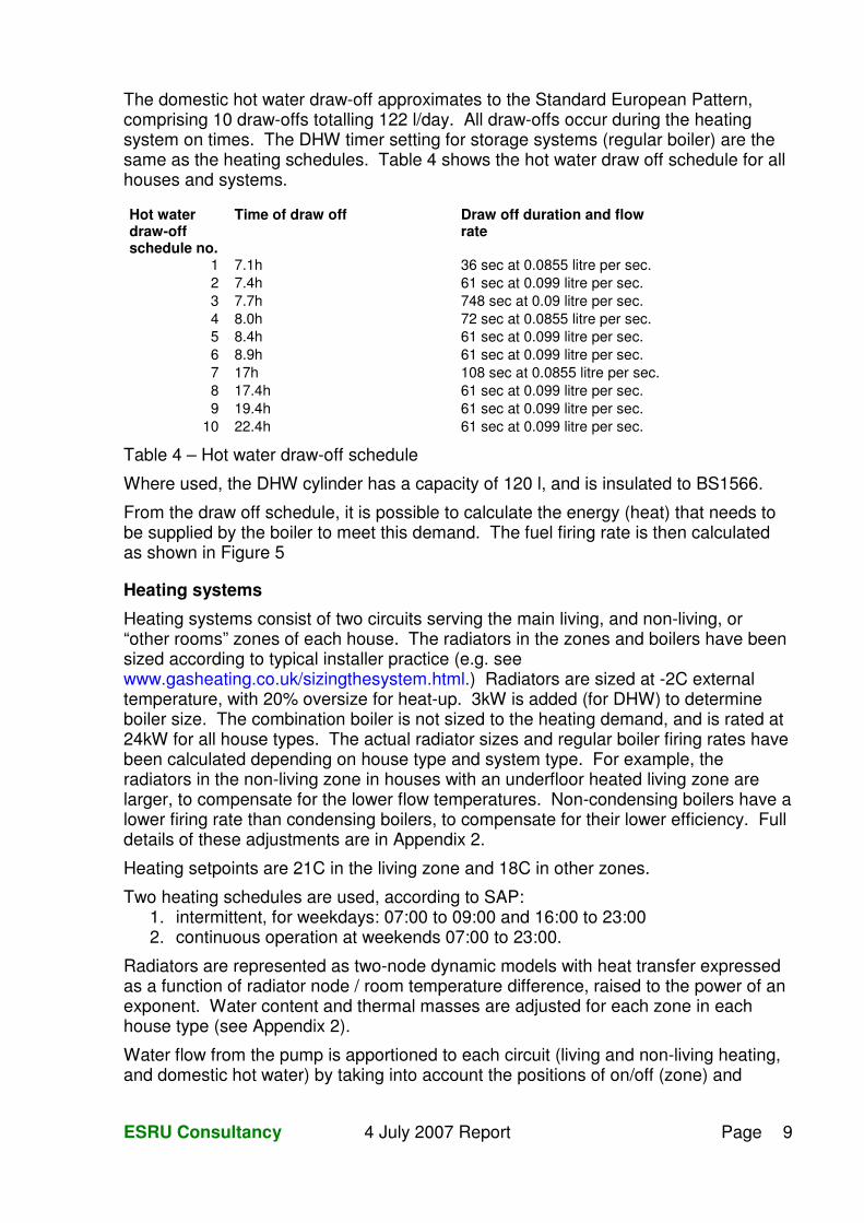
Gas condensing Gas non-condensing Oil condensing A1 8.663 -0.03823 2.313 A2 -0.2866 -0.003045 -0.097 A3 0.003865 4.471 x 10⁻⁵ 0.001506 A4 -1.8676 x10⁻⁵ -2.395 x 10⁻⁷ -8.052 x 10⁻⁶ A5 -11.102 -1.893 0 A6 0.2822 0.024 0 A7 -.00177 4.382 x 10⁻⁵ 0 A8 7.626 88.01 80.31 Table 3 - Boiler efficiency curve fit polynomial coefficients
Domestic Hot Water
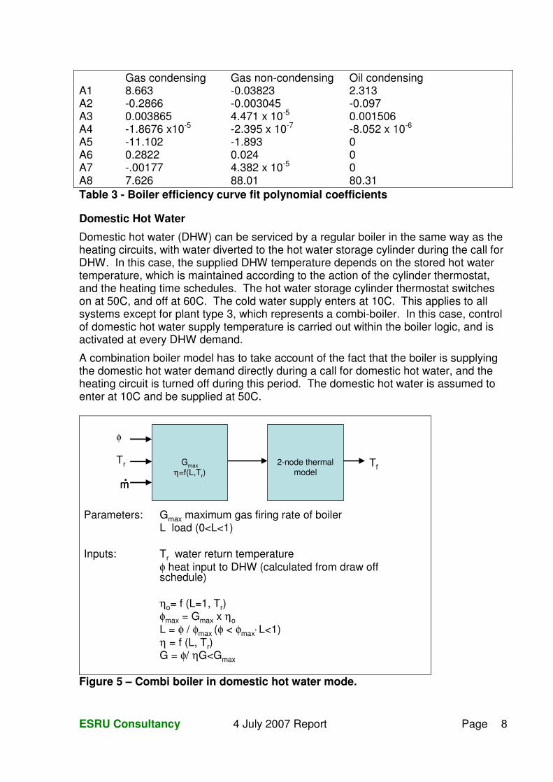
Domestic hot water (DHW) can be serviced by a regular boiler in the same way as the heating circuits, with water diverted to the hot water storage cylinder during the call for DHW. In this case, the supplied DHW temperature depends on the stored hot water temperature, which is maintained according to the action of the cylinder thermostat, and the heating time schedules. The hot water storage cylinder thermostat switches on at 50C, and off at 60C. The cold water supply enters at 10C. This applies to all systems except for plant type 3, which represents a combi-boiler. In this case, control of domestic hot water supply temperature is carried out within the boiler logic, and is activated at every DHW demand.
A combination boiler model has to take account of the fact that the boiler is supplying the domestic hot water demand directly during a call for domestic hot water, and the heating circuit is turned off during this period. The domestic hot water is assumed to enter at 10C and be supplied at 50C.
Parameters: Gmax maximum gas firing rate of boilerL load (0<L<1)
Inputs: Tr water return temperatureφ heat input to DHW (calculated from draw offschedule)
ηo= f (L=1, Tr)φmax = Gmax x ηoL = φ / φmax (φ < φmax
, L<1)η = f (L, Tr)G = φ/ ηG<Gmax
Gmaxη=f(L,Tr)
φ
Tr
m.
m.
2-node thermalmodel
Tf
Figure 5 – Combi boiler in domestic hot water mode.
ESRU Consultancy 4 July 2007 Report Page 9
The domestic hot water draw-off approximates to the Standard European Pattern, comprising 10 draw-offs totalling 122 l/day. All draw-offs occur during the heating system on times. The DHW timer setting for storage systems (regular boiler) are the same as the heating schedules. Table 4 shows the hot water draw off schedule for all houses and systems. Hot water draw-off schedule no.
Time of draw off Draw off duration and flow rate
1 7.1h 36 sec at 0.0855 litre per sec. 2 7.4h 61 sec at 0.099 litre per sec. 3 7.7h 748 sec at 0.09 litre per sec. 4 8.0h 72 sec at 0.0855 litre per sec. 5 8.4h 61 sec at 0.099 litre per sec. 6 8.9h 61 sec at 0.099 litre per sec. 7 17h 108 sec at 0.0855 litre per sec. 8 17.4h 61 sec at 0.099 litre per sec. 9 19.4h 61 sec at 0.099 litre per sec.
10 22.4h 61 sec at 0.099 litre per sec.
Table 4 – Hot water draw-off schedule
Where used, the DHW cylinder has a capacity of 120 l, and is insulated to BS1566.
From the draw off schedule, it is possible to calculate the energy (heat) that needs to be supplied by the boiler to meet this demand. The fuel firing rate is then calculated as shown in Figure 5
Heating systems
Heating systems consist of two circuits serving the main living, and non-living, or “other rooms” zones of each house. The radiators in the zones and boilers have been sized according to typical installer practice (e.g. see www.gasheating.co.uk/sizingthesystem.html.) Radiators are sized at -2C external temperature, with 20% oversize for heat-up. 3kW is added (for DHW) to determine boiler size. The combination boiler is not sized to the heating demand, and is rated at 24kW for all house types. The actual radiator sizes and regular boiler firing rates have been calculated depending on house type and system type. For example, the radiators in the non-living zone in houses with an underfloor heated living zone are larger, to compensate for the lower flow temperatures. Non-condensing boilers have a lower firing rate than condensing boilers, to compensate for their lower efficiency. Full details of these adjustments are in Appendix 2.
Heating setpoints are 21C in the living zone and 18C in other zones.
Two heating schedules are used, according to SAP: 1. intermittent, for weekdays: 07:00 to 09:00 and 16:00 to 23:00 2. continuous operation at weekends 07:00 to 23:00.
Radiators are represented as two-node dynamic models with heat transfer expressed as a function of radiator node / room temperature difference, raised to the power of an exponent. Water content and thermal masses are adjusted for each zone in each house type (see Appendix 2).
Water flow from the pump is apportioned to each circuit (living and non-living heating, and domestic hot water) by taking into account the positions of on/off (zone) and
ESRU Consultancy 4 July 2007 Report Page 10
modulating (TRV) valves. Flows are apportioned according to the relative system sizes to give the correct design temperature drop across radiators. If the pump has to run with no zone calling for heat, the flow goes through a bypass.
Controls
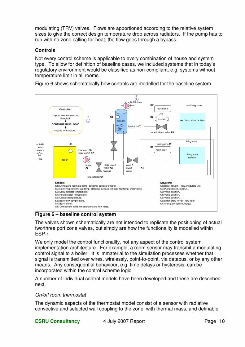
Not every control scheme is applicable to every combination of house and system type. To allow for definition of baseline cases, we included systems that in today’s regulatory environment would be classified as non-compliant, e.g. systems without temperature limit in all rooms.
Figure 6 shows schematically how controls are modelled for the baseline system.
t2
DHW draw A6 S2* non living zone
ORt1 S3 S2
feed at 10oC
zone 2 divert valve A5
living zoneoutside A1 anticipator A7temp S1
sensor flow temp S6 boiler on/off S7
S5
pump DHW divert zone 1 A2 valve A3 divert A4
bypass valve
return temp S4
Sensors: Actuators:S1: Living zone roomstat temp, dB temp, surface temp(s). A1: Boiler (on/off, Tflow, modulate y/n).S2: Non living zone trv stat temp, dB temp, surface temp(s), rad temp, water temp. A2: Pump (on/off, overrun).S3: DHW cylinder temperature. A3: Valve position.S4: Return water temperature. A4: Valve position.S5: Outside temperature. A5: Valve position.S6: Boiler flow temperature. A6: DHW draw (on/off, flow rate).S7: Boiler on/off. A7: Anticipator (on/off, watts).ST: Component node temperatures and flow rates.
trvstat
living zone radiator
non living zone radiator
roomstat 1
roomstat 2
trv stat
boiler
cylinder
Controller:
...inputs from sensors and timeclock
CONFIGURABLE LOGIC
outputs to actuators...
Figure 6 – baseline control system
The valves shown schematically are not intended to replicate the positioning of actual two/three port zone valves, but simply are how the functionality is modelled within ESP-r.
We only model the control functionality, not any aspect of the control system implementation architecture. For example, a room sensor may transmit a modulating control signal to a boiler. It is immaterial to the simulation processes whether that signal is transmitted over wires, wirelessly, point-to-point, via databus, or by any other means. Any consequential behaviour, e.g. time delays or hysteresis, can be incorporated within the control scheme logic.
A number of individual control models have been developed and these are described next.
On/off room thermostat
The dynamic aspects of the thermostat model consist of a sensor with radiative convective and selected wall coupling to the zone, with thermal mass, and definable
ESRU Consultancy 4 July 2007 Report Page 11
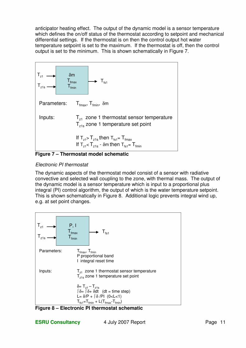
anticipator heating effect. The output of the dynamic model is a sensor temperature which defines the on/off status of the thermostat according to setpoint and mechanical differential settings. If the thermostat is on then the control output hot water temperature setpoint is set to the maximum. If the thermostat is off, then the control output is set to the minimum. This is shown schematically in Figure 7.
Parameters: Tfmax, Tfmin, δm
Inputs: Tz1 zone 1 thermostat sensor temperatureTz1s zone 1 temperature set point
If Tz1> Tz1s then Tfs1= Tfmax
If Tz1< Tz1s - δm then Tfs1= Tfmin
δmTfmaxTfmin
Tfs1
Tz1
Tz1s
Figure 7 – Thermostat model schematic
Electronic PI thermostat
The dynamic aspects of the thermostat model consist of a sensor with radiative convective and selected wall coupling to the zone, with thermal mass. The output of the dynamic model is a sensor temperature which is input to a proportional plus integral (PI) control algorithm, the output of which is the water temperature setpoint. This is shown schematically in Figure 8. Additional logic prevents integral wind up, e.g. at set point changes.
Parameters: Tfmax, TfminP proportional bandI integral reset time
Inputs: Tz1 zone 1 thermostat sensor temperatureTz1s zone 1 temperature set point
δ= Tz1 – Tz1s� δ= � δ+ δdt (dt = time step)L= δ/P + � δ /PI (0<L<1)Tfs1=Tfmin + L(Tfmax-Tfmin)
P, ITfmaxTfmin
Tfs1
Tz1
Tz1s
Figure 8 – Electronic PI thermostat schematic
ESRU Consultancy 4 July 2007 Report Page 12
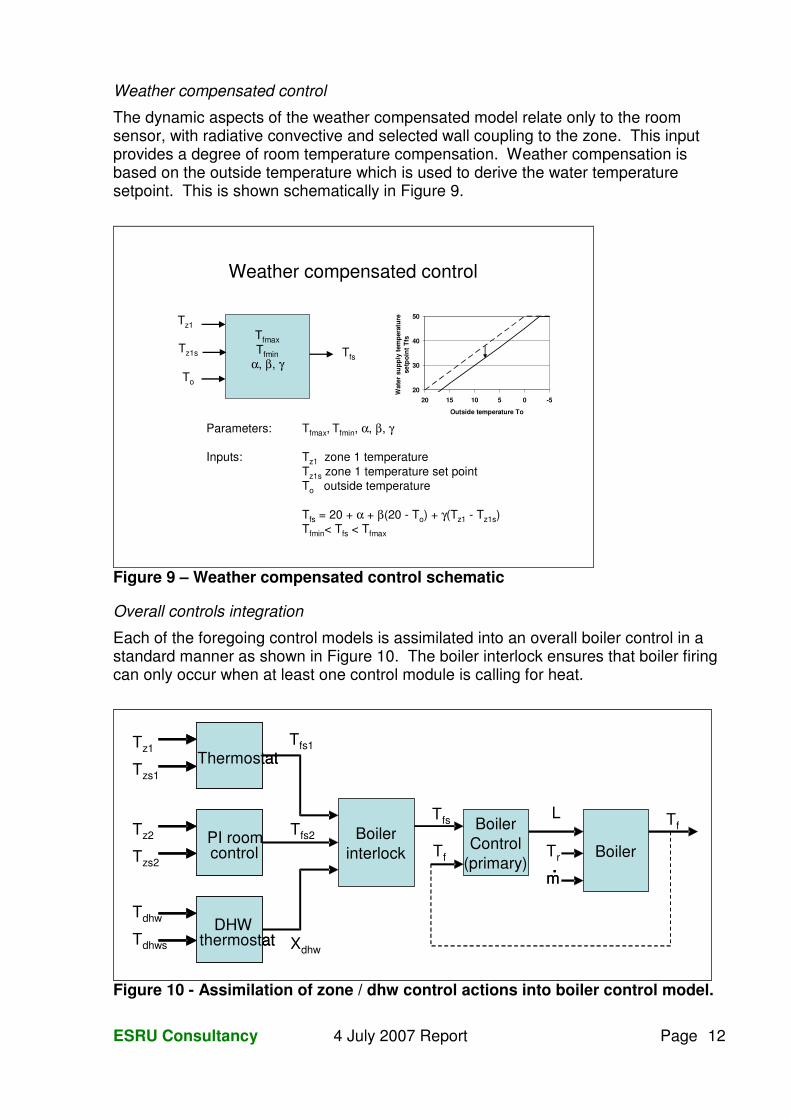
Weather compensated control
The dynamic aspects of the weather compensated model relate only to the room sensor, with radiative convective and selected wall coupling to the zone. This input provides a degree of room temperature compensation. Weather compensation is based on the outside temperature which is used to derive the water temperature setpoint. This is shown schematically in Figure 9.
Weather compensated control
TfmaxTfmin
α, β, γTfs
To
Tz1
Tz1s
20
30
40
50
-505101520
Outside temperature To
Wat
er s
upp
ly t
empe
ratu
re
setp
oin
t Tf
s
Parameters: Tfmax, Tfmin, α, β, γ
Inputs: Tz1 zone 1 temperatureTz1s zone 1 temperature set pointTo outside temperature
Tfs = 20 + α + β(20 - To) + γ(Tz1 - Tz1s)Tfmin< Tfs < Tfmax
Figure 9 – Weather compensated control schematic
Overall controls integration
Each of the foregoing control models is assimilated into an overall boiler control in a standard manner as shown in Figure 10. The boiler interlock ensures that boiler firing can only occur when at least one control module is calling for heat.
Figure 10 - Assimilation of zone / dhw control actions into boiler control model.
ThermostatThermostat
PI roomcontrolPI roomcontrol
DHWthermostat
DHWthermostat
Boilerinterlock
Boiler Control
(primary) Boiler
Tz1
Tz2
Tdhw
Tzs1
Tzs2
Tdhws
Tfs1
Tfs2
X dhw
Tfs Tf
Tr m.
m.
Tf
L
ESRU Consultancy 4 July 2007 Report Page 13
Component Description Units Value Comment
Circulating pump
1node model
Maximum flow rate kg/s 0.214 varies by house Open circuit flow rate kg/s 1.0 varies by house Bypass setting fraction of
maximum pump flow
0.33
total mass kg 5 Mass weighted average specific
heat J/kgK 2250
Heat transfer coefficient (to containment)
W/K 0.2
Total absorbed power W 150 Living zone radiator
2 node model with exponent
Nominal heat emission W 3,528 varies by house and system
Nominal supply temperature C 80 varies by system Nominal return temperature C 70 varies by system Nominal environment
temperarure C 21
Heat transfer exponent - 1.21 varies by system Mass kg 71 varies by house
and system Non living zone radiator
2 node model with exponent
Nominal heat emission W 5,424 varies by house and system
Nominal supply temperature C 80 varies by system Nominal return temperature C 70 varies by system Nominal environment
temperarure C 18
Heat transfer exponent - 1.21 varies by system Mass kg 109 varies by house
and system Hot water cylinder / combi heat exchanger
2 node model
total mass kg 120 varies by system Mass weighted average specific
heat J/kgK 4180
Heat transfer coefficient (to containment)
W/K 1.03 varies by system
Mass of water in coil kg 15 varies by system Internal heat transfer area m^2 0.5 varies by system Internal heat transfer coefficient W/m^2K 12,000 varies by system External heat transfer area m^2 0.55 varies by system External heat transfer coefficient W/m^2K 1,200 varies by system
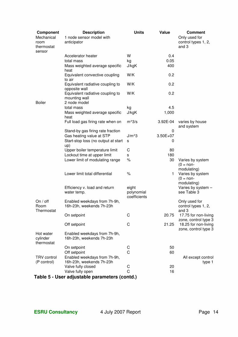
Table 5 - User adjustable parameters
ESRU Consultancy 4 July 2007 Report Page 14
Component Description Units Value Comment
Mechanical room thermostat sensor
1 node sensor model with anticipator
Only used for control types 1, 2, and 3
Accelerator heater W 0.4 total mass kg 0.05 Mass weighted average specific
heat J/kgK 400
Equivalent convective coupling to air
W/K 0.2
Equivalent radiative coupling to opposite wall
W/K 0.2
Equivalent radiative coupling to mounting wall
W/K 0.2
Boiler 2 node model total mass kg 4.5 Mass weighted average specific
heat J/kgK 1,000
Full load gas firing rate when on m^3/s 3.92E-04 varies by house and system
Stand-by gas firing rate fraction 0 Gas heating value at STP J/m^3 3.50E+07 Start-stop loss (no output at start
up) s 0
Upper boiler temperature limit C 80 Lockout time at upper limit s 180 Lower limit of modulating range % 30 Varies by system
(0 = non-modulating)
Lower limit total differential % 1 Varies by system (0 = non-modulating)
Efficiency v. load and return water temp.
eight polynomial coefficients
Varies by system – see Table 3
On / off Room Thermostat
Enabled weekdays from 7h-9h, 16h-23h, weekends 7h-23h
Only used for control types 1, 2, and 3
On setpoint C 20.75 17.75 for non-living zone, control type 3
Off setpoint C 21.25 18.25 for non-living zone, control type 3
Hot water cylinder thermostat
Enabled weekdays from 7h-9h, 16h-23h, weekends 7h-23h
On setpoint C 50 Off setpoint C 60
TRV control (P control)
Enabled weekdays from 7h-9h, 16h-23h, weekends 7h-23h
All except control type 1
Valve fully closed C 20 Valve fully open C 16
Table 5 - User adjustable parameters (contd.)
ESRU Consultancy 4 July 2007 Report Page 15
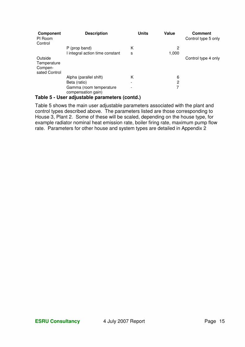
Component Description Units Value Comment
PI Room Control
Control type 5 only
P (prop band) K 2 I integral action time constant s 1,000
Outside Temperature Compen-sated Control
Control type 4 only
Alpha (parallel shift) K 6 Beta (ratio) - 2 Gamma (room temperature
compensation gain) - 7
Table 5 - User adjustable parameters (contd.)
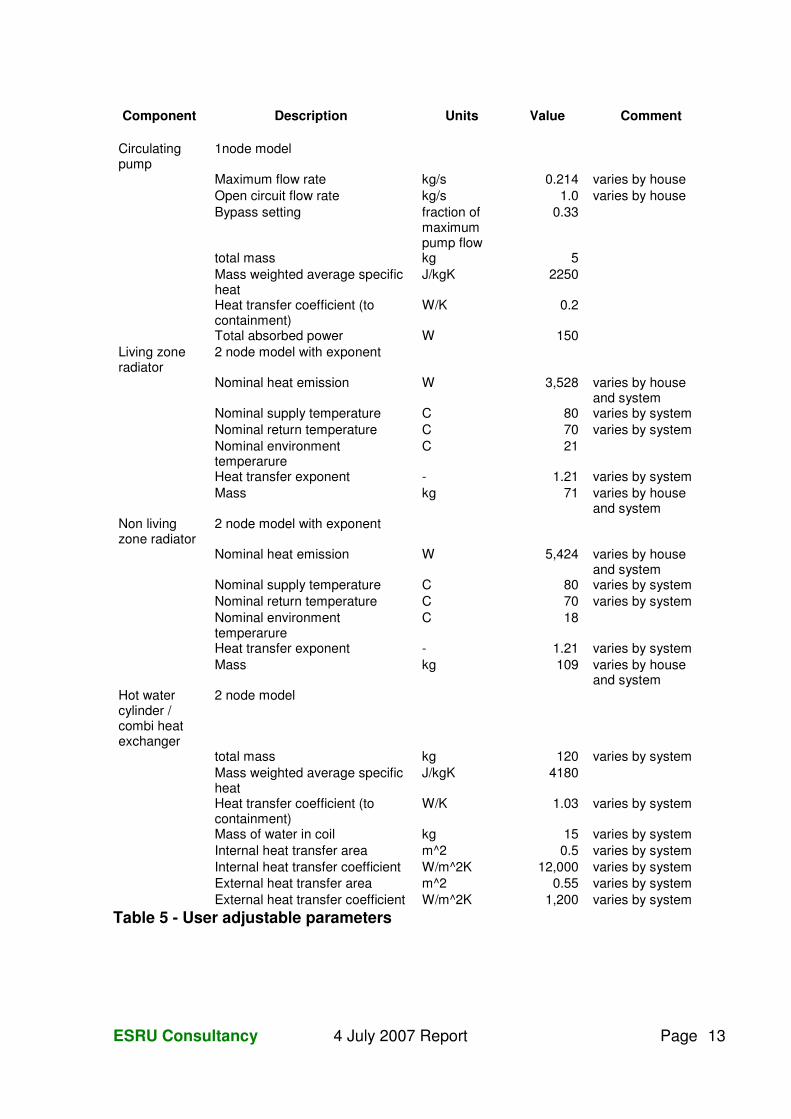
Table 5 shows the main user adjustable parameters associated with the plant and control types described above. The parameters listed are those corresponding to House 3, Plant 2. Some of these will be scaled, depending on the house type, for example radiator nominal heat emission rate, boiler firing rate, maximum pump flow rate. Parameters for other house and system types are detailed in Appendix 2
ESRU Consultancy 4 July 2007 Report Page 16
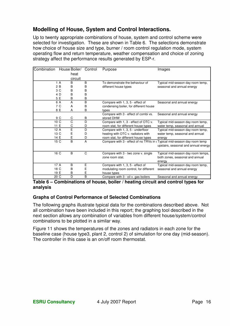
Modelling of House, System and Control Interactions. Up to twenty appropriate combinations of house, system and control scheme were selected for investigation. These are shown in Table 6. The selections demonstrate how choice of house size and type, burner / room control regulation mode, system operating flow and return temperature, weather compensation and choice of zoning strategy affect the performance results generated by ESP-r. Combination House Boiler/
heat circuit
Control Purpose Images
1 A B B2 B B B3 C B B4 D B B5 E B B6 A A B7 C A B8 E A B
9 C C BCompare with 3 - effect of combi vs. stored DHW
Seasonal and annual energy
10 C C D11 E C D12 A E D13 C E D14 E E D15 C B A Compare with 3 - effect of no TRVs in other roomsTypical mid-season day room temp
upstairs, seasonal and annual energy
16 C B C Compare with 3 - two zone v. single zone room stat.
Typical mid-season day room temps, both zones, seasonal and annual energy
17 A B E18 C B E19 E B E20 C D B Compare with 3 - oil v. gas boilers Seasonal and annual energy
Compare with 1, 3, 5 - effect of modulating room control, for different house types
Typical mid-season day room temp, seasonal and annual energy
Seasonal and annual energy
Typical mid-season day room temp, seasonal and annual energy
Compare with 1, 3 - effect of OTC v. room stat, for different house types
Typical mid-season day room temp, water temp, seasonal and annual
Compare with 1, 3, 5 - underfloor heating with OTC v. radiators with room stat, for different house types
Typical mid-season day room temp, water temp, seasonal and annual energy
To demonstrate the behaviour of different house types
Compare with 1, 3, 5 - effect of condensing boiler, for different house types
Table 6 – Combinations of house, boiler / heating circuit and control types for analysis
Graphs of Control Performance of Selected Combinations
The following graphs illustrate typical data for the combinations described above. Not all combination have been included in this report; the graphing tool described in the next section allows any combination of variables from different house/system/control combinations to be plotted in a similar way.
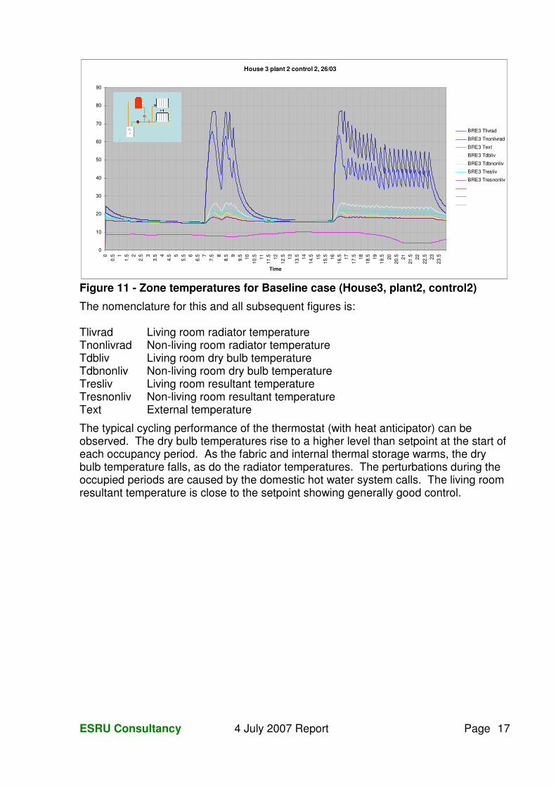
Figure 11 shows the temperatures of the zones and radiators in each zone for the baseline case (house type3, plant 2, control 2) of simulation for one day (mid-season). The controller in this case is an on/off room thermostat.
ESRU Consultancy 4 July 2007 Report Page 17
House 3 plant 2 control 2, 26/03
0
10
20
30
40
50
60
70
80
90
00.
5 11.
5 22.
5 33.
5 44.
5 55.
5 66.
5 77.
5 88.
5 99.
5 1010
.5 1111
.5 1212
.5 1313
.5 1414
.5 1515
.5 1616
.5 1717
.5 1818
.5 1919
.5 2020
.5 2121
.5 2222
.5 2323
.5
Time
BRE3 Tlivrad
BRE3 Tnonlivrad
BRE3 Text
BRE3 Tdbliv
BRE3 Tdbnonliv
BRE3 Tresliv
BRE3 Tresnonliv
Figure 11 - Zone temperatures for Baseline case (House3, plant2, control2)
The nomenclature for this and all subsequent figures is: Tlivrad Living room radiator temperature Tnonlivrad Non-living room radiator temperature Tdbliv Living room dry bulb temperature Tdbnonliv Non-living room dry bulb temperature Tresliv Living room resultant temperature Tresnonliv Non-living room resultant temperature Text External temperature
The typical cycling performance of the thermostat (with heat anticipator) can be observed. The dry bulb temperatures rise to a higher level than setpoint at the start of each occupancy period. As the fabric and internal thermal storage warms, the dry bulb temperature falls, as do the radiator temperatures. The perturbations during the occupied periods are caused by the domestic hot water system calls. The living room resultant temperature is close to the setpoint showing generally good control.
ESRU Consultancy 4 July 2007 Report Page 18
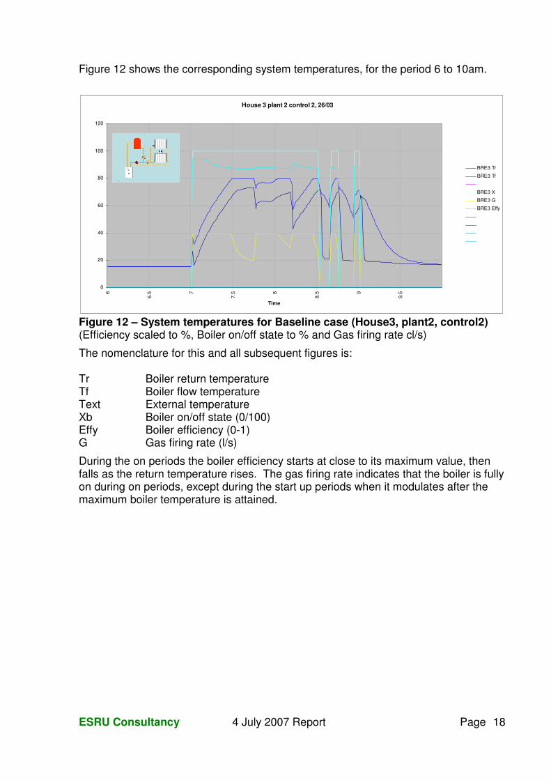
Figure 12 shows the corresponding system temperatures, for the period 6 to 10am.
House 3 plant 2 control 2, 26/03
0
20
40
60
80
100
120
6
6.5 7
7.5 8
8.5 9
9.5
Time
BRE3 Tr
BRE3 Tf
BRE3 X
BRE3 G
BRE3 Effy
Figure 12 – System temperatures for Baseline case (House3, plant2, control2) (Efficiency scaled to %, Boiler on/off state to % and Gas firing rate cl/s)
The nomenclature for this and all subsequent figures is: Tr Boiler return temperature Tf Boiler flow temperature Text External temperature Xb Boiler on/off state (0/100) Effy Boiler efficiency (0-1) G Gas firing rate (l/s)
During the on periods the boiler efficiency starts at close to its maximum value, then falls as the return temperature rises. The gas firing rate indicates that the boiler is fully on during on periods, except during the start up periods when it modulates after the maximum boiler temperature is attained.
ESRU Consultancy 4 July 2007 Report Page 19
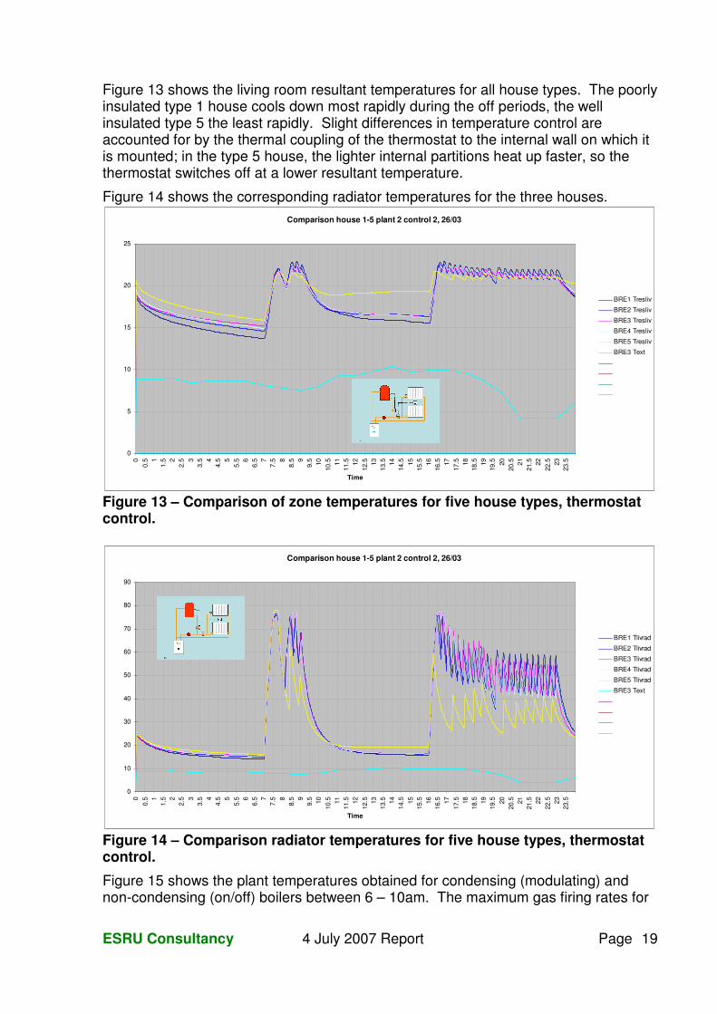
Figure 13 shows the living room resultant temperatures for all house types. The poorly insulated type 1 house cools down most rapidly during the off periods, the well insulated type 5 the least rapidly. Slight differences in temperature control are accounted for by the thermal coupling of the thermostat to the internal wall on which it is mounted; in the type 5 house, the lighter internal partitions heat up faster, so the thermostat switches off at a lower resultant temperature.
Figure 14 shows the corresponding radiator temperatures for the three houses. Comparison house 1-5 plant 2 control 2, 26/03
0
5
10
15
20
25
00.
5 11.
5 22.
5 33.
5 44.
5 55.
5 66.
5 77.
5 88.
5 99.
5 1010
.5 1111
.5 1212
.5 1313
.5 1414
.5 1515
.5 1616
.5 1717
.5 1818
.5 1919
.5 2020
.5 2121
.5 2222
.5 2323
.5
Time
BRE1 Tresliv
BRE2 Tresliv
BRE3 Tresliv
BRE4 Tresliv
BRE5 Tresliv
BRE3 Text
Figure 13 – Comparison of zone temperatures for five house types, thermostat control.
Comparison house 1-5 plant 2 control 2, 26/03
0
10
20
30
40
50
60
70
80
90
00.
5 11.
5 22.
5 33.
5 44.
5 55.
5 66.
5 77.
5 88.
5 99.
5 1010
.5 1111
.5 1212
.5 1313
.5 1414
.5 1515
.5 1616
.5 1717
.5 1818
.5 1919
.5 2020
.5 2121
.5 2222
.5 2323
.5
Time
BRE1 Tlivrad
BRE2 Tlivrad
BRE3 Tlivrad
BRE4 Tlivrad
BRE5 Tlivrad
BRE3 Text
Figure 14 – Comparison radiator temperatures for five house types, thermostat control.
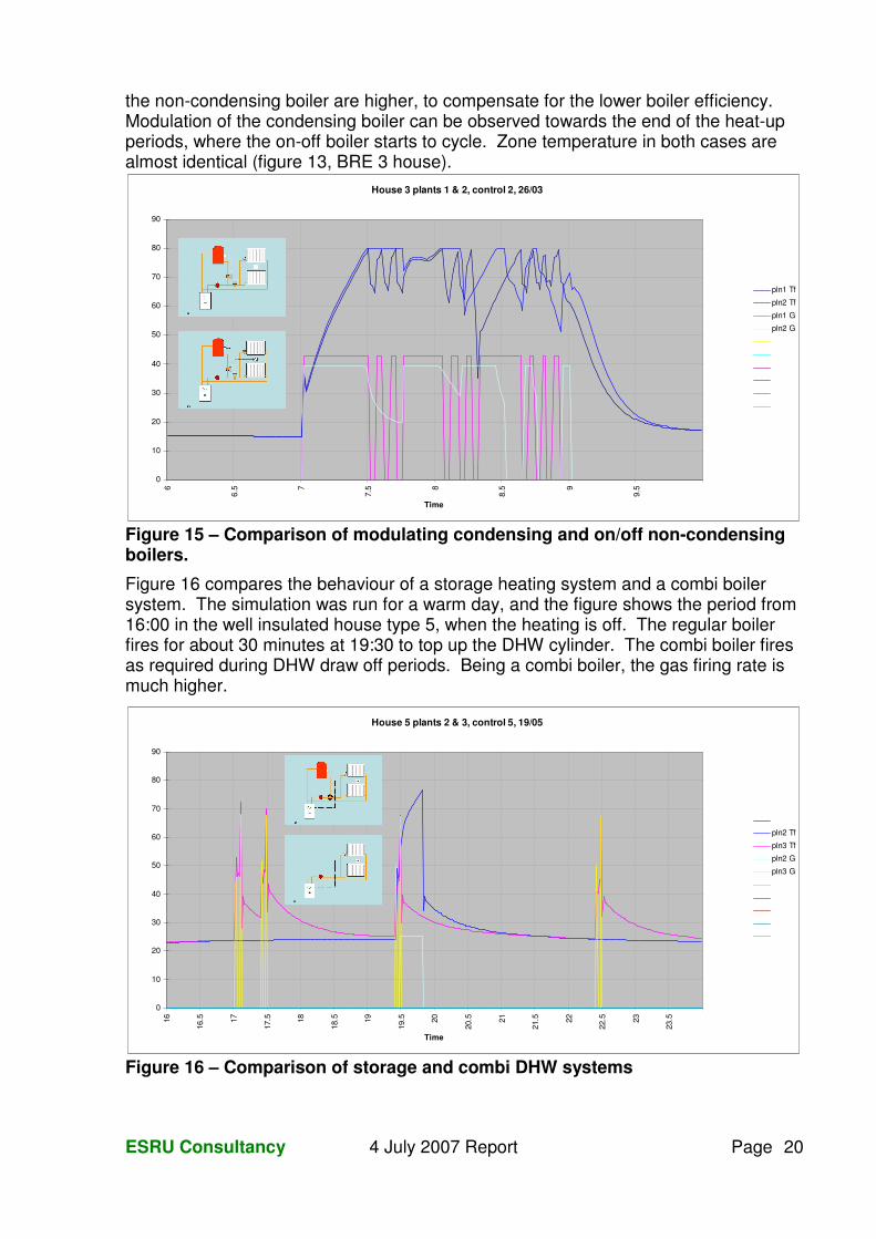
Figure 15 shows the plant temperatures obtained for condensing (modulating) and non-condensing (on/off) boilers between 6 – 10am. The maximum gas firing rates for
ESRU Consultancy 4 July 2007 Report Page 20
the non-condensing boiler are higher, to compensate for the lower boiler efficiency. Modulation of the condensing boiler can be observed towards the end of the heat-up periods, where the on-off boiler starts to cycle. Zone temperature in both cases are almost identical (figure 13, BRE 3 house).
House 3 plants 1 & 2, control 2, 26/03
0
10
20
30
40
50
60
70
80
90
6
6.5 7
7.5 8
8.5 9
9.5
Time
pln1 Tf
pln2 Tf
pln1 G
pln2 G
Figure 15 – Comparison of modulating condensing and on/off non-condensing boilers.
Figure 16 compares the behaviour of a storage heating system and a combi boiler system. The simulation was run for a warm day, and the figure shows the period from 16:00 in the well insulated house type 5, when the heating is off. The regular boiler fires for about 30 minutes at 19:30 to top up the DHW cylinder. The combi boiler fires as required during DHW draw off periods. Being a combi boiler, the gas firing rate is much higher.
House 5 plants 2 & 3, control 5, 19/05
0
10
20
30
40
50
60
70
80
90
16
16.5 17
17.5 18
18.5 19
19.5 20
20.5 21
21.5 22
22.5 23
23.5
Time
pln2 Tf
pln3 Tf
pln2 G
pln3 G
Figure 16 – Comparison of storage and combi DHW systems
ESRU Consultancy 4 July 2007 Report Page 21
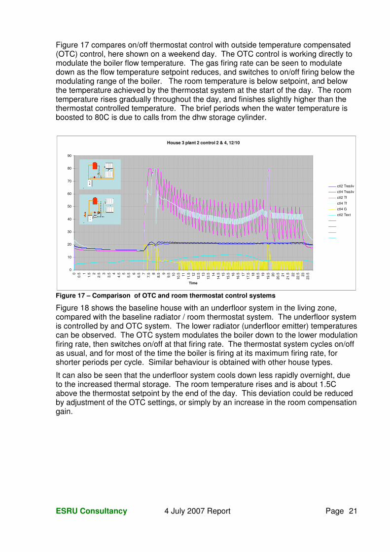
Figure 17 compares on/off thermostat control with outside temperature compensated (OTC) control, here shown on a weekend day. The OTC control is working directly to modulate the boiler flow temperature. The gas firing rate can be seen to modulate down as the flow temperature setpoint reduces, and switches to on/off firing below the modulating range of the boiler. The room temperature is below setpoint, and below the temperature achieved by the thermostat system at the start of the day. The room temperature rises gradually throughout the day, and finishes slightly higher than the thermostat controlled temperature. The brief periods when the water temperature is boosted to 80C is due to calls from the dhw storage cylinder.
House 3 plant 2 control 2 & 4, 12/10
0
10
20
30
40
50
60
70
80
90
00.
5 11.
5 22.
5 33.
5 44.
5 55.
5 66.
5 77.
5 88.
5 99.
5 1010
.5 1111
.5 1212
.5 1313
.5 1414
.5 1515
.5 1616
.5 1717
.5 1818
.5 1919
.5 2020
.5 2121
.5 2222
.5 2323
.5
Time
ctl2 Tresliv
ctl4 Tresliv
ctl2 Tf
ctl4 Tf
ctl4 G
ctl2 Text
Figure 17 – Comparison of OTC and room thermostat control systems
Figure 18 shows the baseline house with an underfloor system in the living zone, compared with the baseline radiator / room thermostat system. The underfloor system is controlled by and OTC system. The lower radiator (underfloor emitter) temperatures can be observed. The OTC system modulates the boiler down to the lower modulation firing rate, then switches on/off at that firing rate. The thermostat system cycles on/off as usual, and for most of the time the boiler is firing at its maximum firing rate, for shorter periods per cycle. Similar behaviour is obtained with other house types.
It can also be seen that the underfloor system cools down less rapidly overnight, due to the increased thermal storage. The room temperature rises and is about 1.5C above the thermostat setpoint by the end of the day. This deviation could be reduced by adjustment of the OTC settings, or simply by an increase in the room compensation gain.
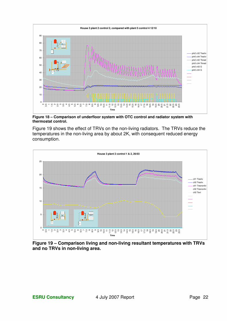
ESRU Consultancy 4 July 2007 Report Page 22
House 3 plant 2 control 2, compared with plant 5 control 4 12/10
0
10
20
30
40
50
60
70
80
90
00.
5 11.
5 22.
5 33.
5 44.
5 55.
5 66.
5 77.
5 88.
5 99.
5 1010
.5 1111
.5 1212
.5 1313
.5 1414
.5 1515
.5 1616
.5 1717
.5 1818
.5 1919
.5 2020
.5 2121
.5 2222
.5 2323
.5
Time
pln2 ctl2 Tresliv
pln5 ctl4 Tresliv
pln2 ctl2 Tlivrad
pln5 ctl4 Tlivrad
pln2 ctl2 G
pln5 ctl4 G
Figure 18 – Comparison of underfloor system with OTC control and radiator system with thermostat control.
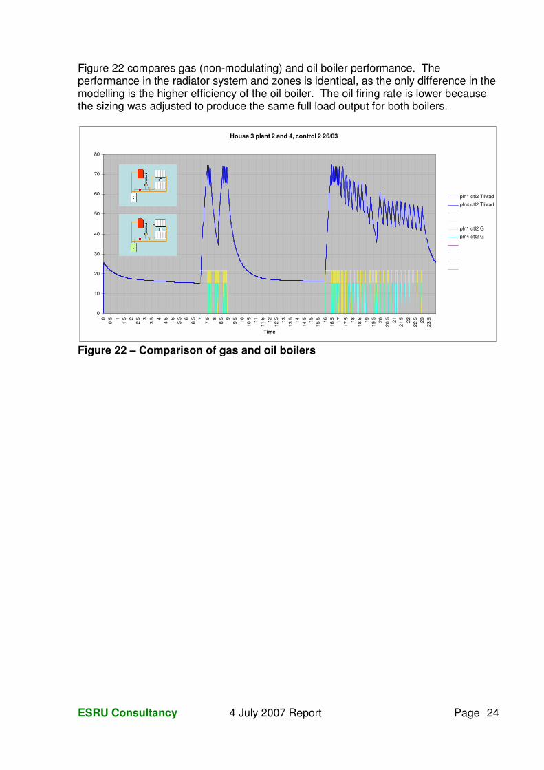
Figure 19 shows the effect of TRVs on the non-living radiators. The TRVs reduce the temperatures in the non-living area by about 2K, with consequent reduced energy consumption.
House 3 plant 2 control 1 & 2, 26/03
0
5
10
15
20
25
00.
5 11.
5 22.
5 33.
5 44.
5 55.
5 66.
5 77.
5 88.
5 99.
5 1010
.5 1111
.5 1212
.5 1313
.5 1414
.5 1515
.5 1616
.5 1717
.5 1818
.5 1919
.5 2020
.5 2121
.5 2222
.5 2323
.5
Time
ctl1 Tresliv
ctl2 Tresliv
ctl1 Tresnonliv
ctl2 Tresnonliv
ctl2 Text
Figure 19 – Comparison living and non-living resultant temperatures with TRVs and no TRVs in non-living area.

ESRU Consultancy 4 July 2007 Report Page 23
Figure 20 shows the operation of thermostats in both the living and non-living zones. The thermostats cycle at different rates because of the different loadings in each zone. The boiler fires when either room stat is calling for heat.
House 3 plant 2 control 3 26/03
0
10
20
30
40
50
60
70
80
16
16.5 17
17.5 18
18.5
Time
pln2 ctl3 Tresliv
pln2 ctl3 Tresnonliv
pln2 ctl3 Tlivrad
pln2 ctl3 Tnonlivrad
pln2 ctl3 G
Figure 20 – Two zone thermostat control
Figure 21 shows the control of room temperature using a PI controller, compared to an on/off thermostat. The room temperature reaches set point and is closely controlled due to the I action. This results in a lower radiator temperature. There is also less boiler switching, as with OTC control, due to the direct modulation of the boiler.
House 3 plant 2 control 2 and 5 26/03
0
10
20
30
40
50
60
70
80
90
00.
5 11.
5 22.
5 33.
5 44.
5 55.
5 66.
5 77.
5 88.
5 99.
5 1010
.5 1111
.5 1212
.5 1313
.5 1414
.5 1515
.5 1616
.5 1717
.5 1818
.5 1919
.5 2020
.5 2121
.5 2222
.5 2323
.5
Time
pln2 ctl2 Tresliv
pln2 ctl5 Tresliv
pln2 ctl2 Tlivrad
pln2 ctl5 Tlivrad
pln2 ctl2 G
pln2 ctl5 G
Figure 21 – Comparison of thermostat and PI room control.
ESRU Consultancy 4 July 2007 Report Page 24
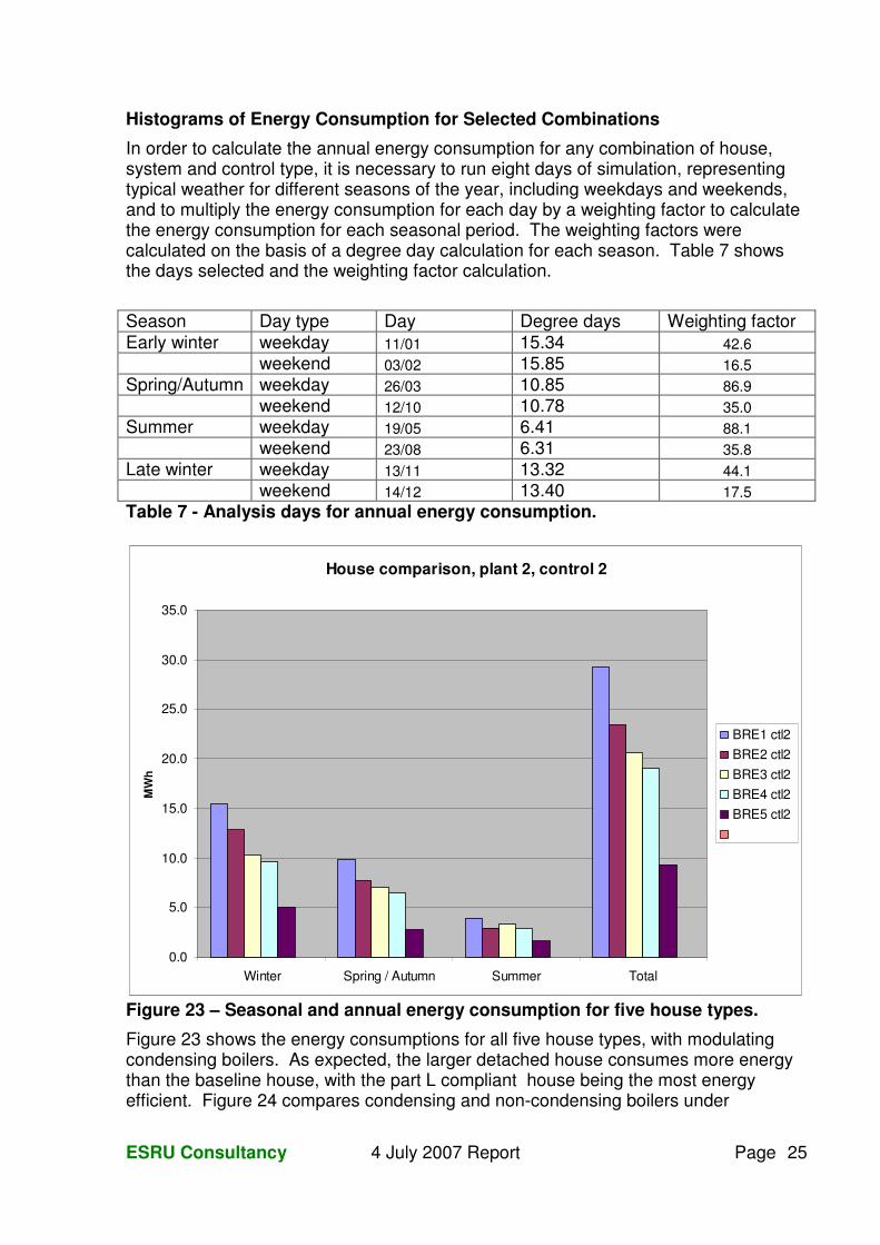
Figure 22 compares gas (non-modulating) and oil boiler performance. The performance in the radiator system and zones is identical, as the only difference in the modelling is the higher efficiency of the oil boiler. The oil firing rate is lower because the sizing was adjusted to produce the same full load output for both boilers.
House 3 plant 2 and 4, control 2 26/03
0
10
20
30
40
50
60
70
80
00.
5 11.
5 22.
5 33.
5 44.
5 55.
5 66.
5 77.
5 88.
5 99.
5 1010
.5 1111
.5 1212
.5 1313
.5 1414
.5 1515
.5 1616
.5 1717
.5 1818
.5 1919
.5 2020
.5 2121
.5 2222
.5 2323
.5
Time
pln1 ctl2 Tlivrad
pln4 ctl2 Tlivrad
pln1 ctl2 G
pln4 ctl2 G
Figure 22 – Comparison of gas and oil boilers
ESRU Consultancy 4 July 2007 Report Page 25
Histograms of Energy Consumption for Selected Combinations
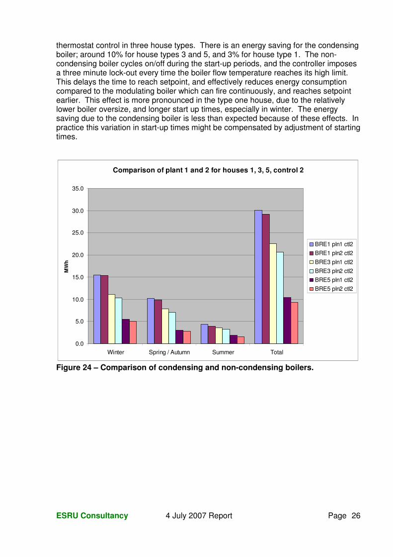
In order to calculate the annual energy consumption for any combination of house, system and control type, it is necessary to run eight days of simulation, representing typical weather for different seasons of the year, including weekdays and weekends, and to multiply the energy consumption for each day by a weighting factor to calculate the energy consumption for each seasonal period. The weighting factors were calculated on the basis of a degree day calculation for each season. Table 7 shows the days selected and the weighting factor calculation.
Season Day type Day Degree days Weighting factor Early winter weekday 11/01 15.34 42.6 weekend 03/02 15.85 16.5 Spring/Autumn weekday 26/03 10.85 86.9 weekend 12/10 10.78 35.0 Summer weekday 19/05 6.41 88.1 weekend 23/08 6.31 35.8 Late winter weekday 13/11 13.32 44.1 weekend 14/12 13.40 17.5 Table 7 - Analysis days for annual energy consumption.
House comparison, plant 2, control 2
0.0
5.0
10.0
15.0
20.0
25.0
30.0
35.0
Winter Spring / Autumn Summer Total
MW
h
BRE1 ctl2 BRE2 ctl2 BRE3 ctl2 BRE4 ctl2 BRE5 ctl2
Figure 23 – Seasonal and annual energy consumption for five house types.
Figure 23 shows the energy consumptions for all five house types, with modulating condensing boilers. As expected, the larger detached house consumes more energy than the baseline house, with the part L compliant house being the most energy efficient. Figure 24 compares condensing and non-condensing boilers under
ESRU Consultancy 4 July 2007 Report Page 26
thermostat control in three house types. There is an energy saving for the condensing boiler; around 10% for house types 3 and 5, and 3% for house type 1. The non-condensing boiler cycles on/off during the start-up periods, and the controller imposes a three minute lock-out every time the boiler flow temperature reaches its high limit. This delays the time to reach setpoint, and effectively reduces energy consumption compared to the modulating boiler which can fire continuously, and reaches setpoint earlier. This effect is more pronounced in the type one house, due to the relatively lower boiler oversize, and longer start up times, especially in winter. The energy saving due to the condensing boiler is less than expected because of these effects. In practice this variation in start-up times might be compensated by adjustment of starting times.
Comparison of plant 1 and 2 for houses 1, 3, 5, control 2
0.0
5.0
10.0
15.0
20.0
25.0
30.0
35.0
Winter Spring / Autumn Summer Total
MW
h
BRE1 pln1 ctl2 BRE1 pln2 ctl2 BRE3 pln1 ctl2 BRE3 pln2 ctl2 BRE5 pln1 ctl2 BRE5 pln2 ctl2
Figure 24 – Comparison of condensing and non-condensing boilers.
ESRU Consultancy 4 July 2007 Report Page 27
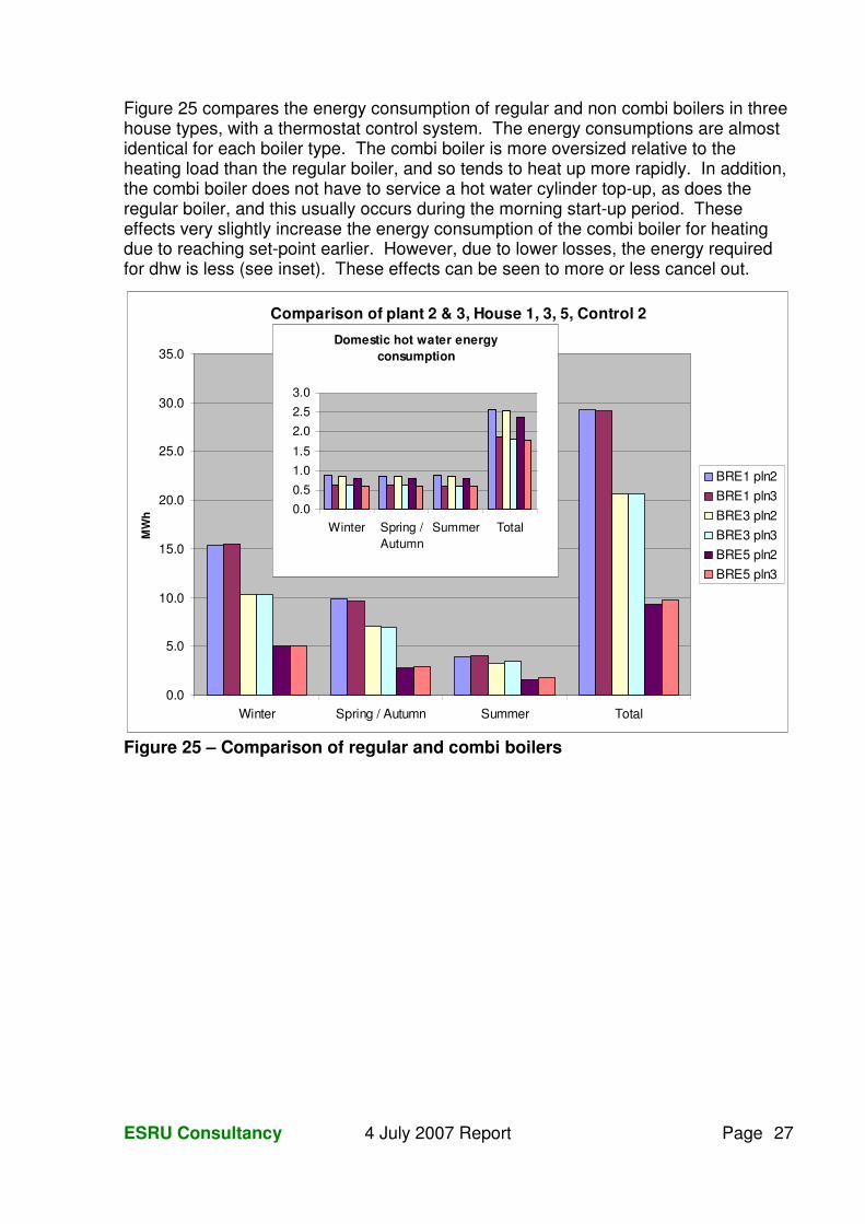
Figure 25 compares the energy consumption of regular and non combi boilers in three house types, with a thermostat control system. The energy consumptions are almost identical for each boiler type. The combi boiler is more oversized relative to the heating load than the regular boiler, and so tends to heat up more rapidly. In addition, the combi boiler does not have to service a hot water cylinder top-up, as does the regular boiler, and this usually occurs during the morning start-up period. These effects very slightly increase the energy consumption of the combi boiler for heating due to reaching set-point earlier. However, due to lower losses, the energy required for dhw is less (see inset). These effects can be seen to more or less cancel out.
Comparison of plant 2 & 3, House 1, 3, 5, Control 2
0.0
5.0
10.0
15.0
20.0
25.0
30.0
35.0
Winter Spring / Autumn Summer Total
MW
h
BRE1 pln2 BRE1 pln3 BRE3 pln2 BRE3 pln3 BRE5 pln2 BRE5 pln3
Figure 25 – Comparison of regular and combi boilers
Domestic hot water energy consumption
0.00.51.01.5
2.02.53.0
Winter Spring /Autumn
Summer Total
ESRU Consultancy 4 July 2007 Report Page 28
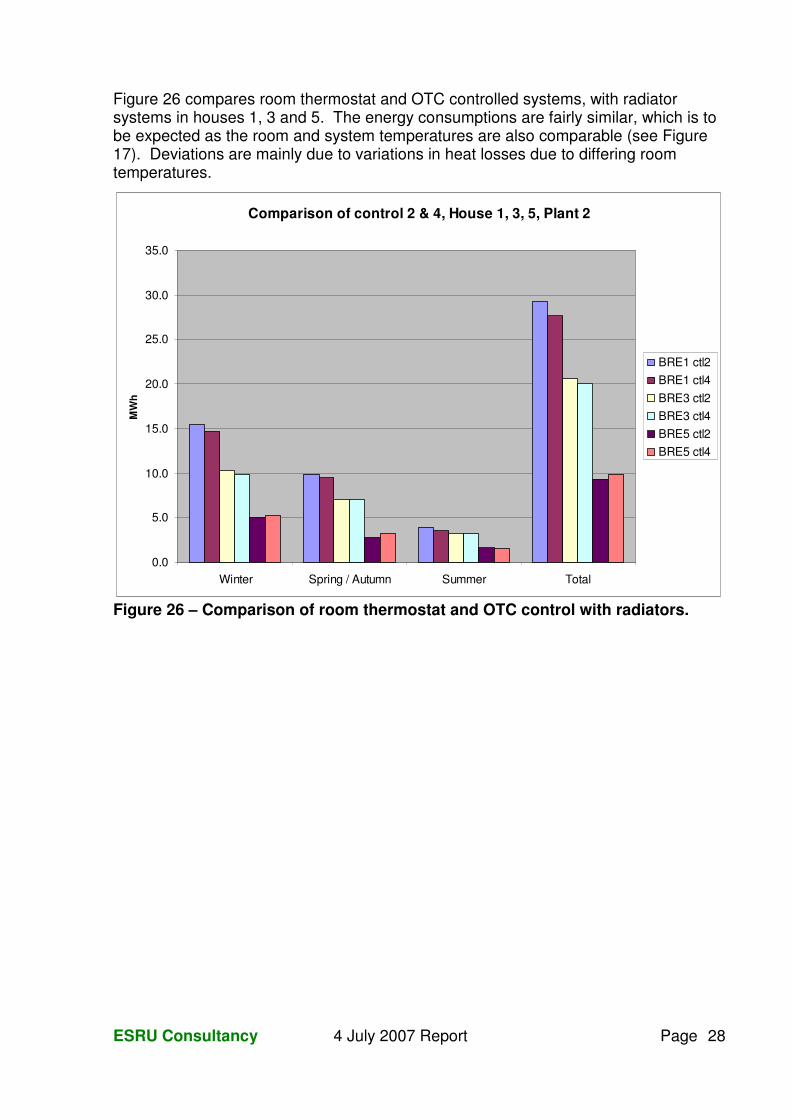
Figure 26 compares room thermostat and OTC controlled systems, with radiator systems in houses 1, 3 and 5. The energy consumptions are fairly similar, which is to be expected as the room and system temperatures are also comparable (see Figure 17). Deviations are mainly due to variations in heat losses due to differing room temperatures.
Comparison of control 2 & 4, House 1, 3, 5, Plant 2
0.0
5.0
10.0
15.0
20.0
25.0
30.0
35.0
Winter Spring / Autumn Summer Total
MW
h
BRE1 ctl2 BRE1 ctl4 BRE3 ctl2 BRE3 ctl4 BRE5 ctl2 BRE5 ctl4
Figure 26 – Comparison of room thermostat and OTC control with radiators.
ESRU Consultancy 4 July 2007 Report Page 29
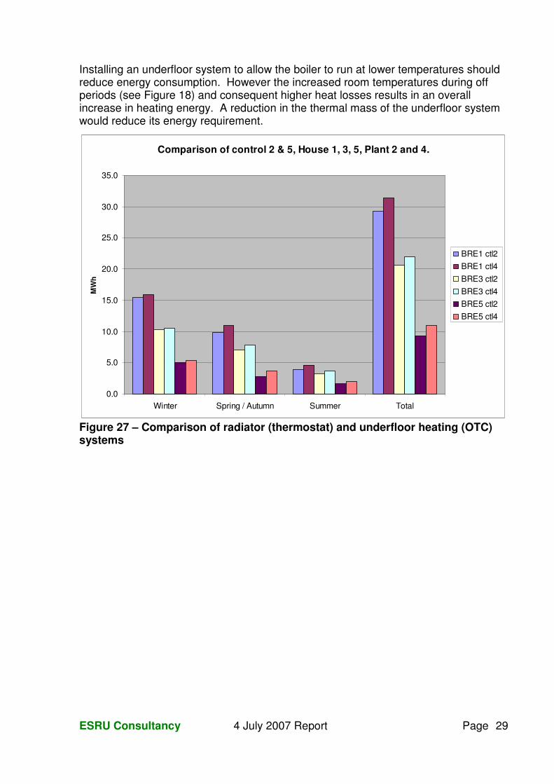
Installing an underfloor system to allow the boiler to run at lower temperatures should reduce energy consumption. However the increased room temperatures during off periods (see Figure 18) and consequent higher heat losses results in an overall increase in heating energy. A reduction in the thermal mass of the underfloor system would reduce its energy requirement.
Comparison of control 2 & 5, House 1, 3, 5, Plant 2 and 4.
0.0
5.0
10.0
15.0
20.0
25.0
30.0
35.0
Winter Spring / Autumn Summer Total
MW
h
BRE1 ctl2 BRE1 ctl4 BRE3 ctl2 BRE3 ctl4 BRE5 ctl2 BRE5 ctl4
Figure 27 – Comparison of radiator (thermostat) and underfloor heating (OTC) systems
ESRU Consultancy 4 July 2007 Report Page 30
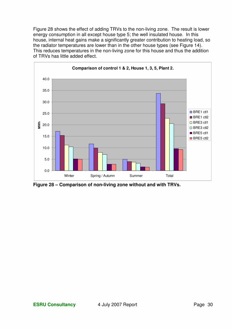
Figure 28 shows the effect of adding TRVs to the non-living zone. The result is lower energy consumption in all except house type 5; the well insulated house. In this house, internal heat gains make a significantly greater contribution to heating load, so the radiator temperatures are lower than in the other house types (see Figure 14). This reduces temperatures in the non-living zone for this house and thus the addition of TRVs has little added effect.
Comparison of control 1 & 2, House 1, 3, 5, Plant 2.
0.0
5.0
10.0
15.0
20.0
25.0
30.0
35.0
40.0
Winter Spring / Autumn Summer Total
MW
h
BRE1 ctl1 BRE1 ctl2 BRE3 ctl1 BRE3 ctl2 BRE5 ctl1 BRE5 ctl2
Figure 28 – Comparison of non-living zone without and with TRVs.
ESRU Consultancy 4 July 2007 Report Page 31
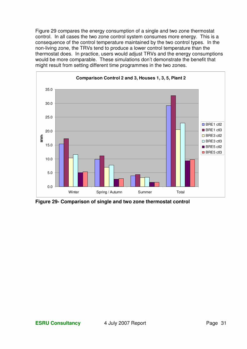
Figure 29 compares the energy consumption of a single and two zone thermostat control. In all cases the two zone control system consumes more energy. This is a consequence of the control temperature maintained by the two control types. In the non-living zone, the TRVs tend to produce a lower control temperature than the thermostat does. In practice, users would adjust TRVs and the energy consumptions would be more comparable. These simulations don’t demonstrate the benefit that might result from setting different time programmes in the two zones.
Comparison Control 2 and 3, Houses 1, 3, 5, Plant 2
0.0
5.0
10.0
15.0
20.0
25.0
30.0
35.0
Winter Spring / Autumn Summer Total
MW
h
BRE1 ctl2 BRE1 ctl3 BRE3 ctl2 BRE3 ctl3 BRE5 ctl2 BRE5 ctl3
Figure 29- Comparison of single and two zone thermostat control
ESRU Consultancy 4 July 2007 Report Page 32
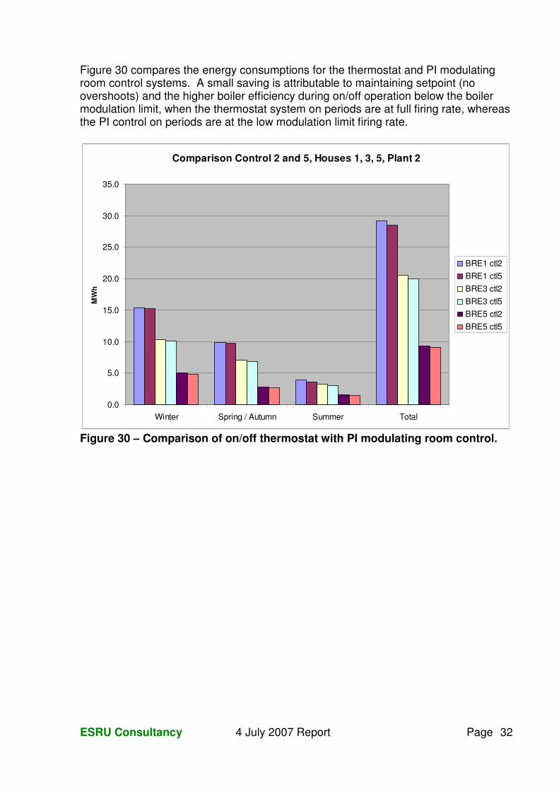
Figure 30 compares the energy consumptions for the thermostat and PI modulating room control systems. A small saving is attributable to maintaining setpoint (no overshoots) and the higher boiler efficiency during on/off operation below the boiler modulation limit, when the thermostat system on periods are at full firing rate, whereas the PI control on periods are at the low modulation limit firing rate.
Comparison Control 2 and 5, Houses 1, 3, 5, Plant 2
0.0
5.0
10.0
15.0
20.0
25.0
30.0
35.0
Winter Spring / Autumn Summer Total
MW
h
BRE1 ctl2 BRE1 ctl5 BRE3 ctl2 BRE3 ctl5 BRE5 ctl2 BRE5 ctl5
Figure 30 – Comparison of on/off thermostat with PI modulating room control.
ESRU Consultancy 4 July 2007 Report Page 33
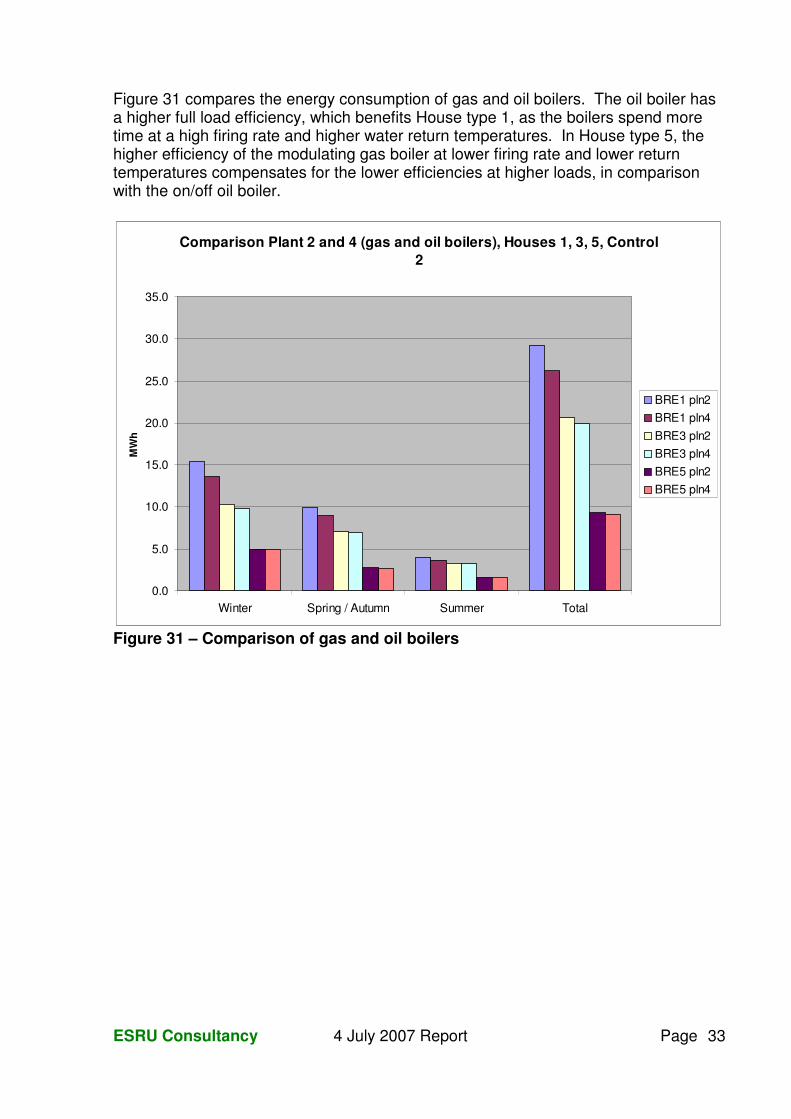
Figure 31 compares the energy consumption of gas and oil boilers. The oil boiler has a higher full load efficiency, which benefits House type 1, as the boilers spend more time at a high firing rate and higher water return temperatures. In House type 5, the higher efficiency of the modulating gas boiler at lower firing rate and lower return temperatures compensates for the lower efficiencies at higher loads, in comparison with the on/off oil boiler.
Comparison Plant 2 and 4 (gas and oil boilers), Houses 1, 3, 5, Control 2
0.0
5.0
10.0
15.0
20.0
25.0
30.0
35.0
Winter Spring / Autumn Summer Total
MW
h
BRE1 pln2 BRE1 pln4 BRE3 pln2 BRE3 pln4 BRE5 pln2 BRE5 pln4
Figure 31 – Comparison of gas and oil boilers
ESRU Consultancy 4 July 2007 Report Page 34
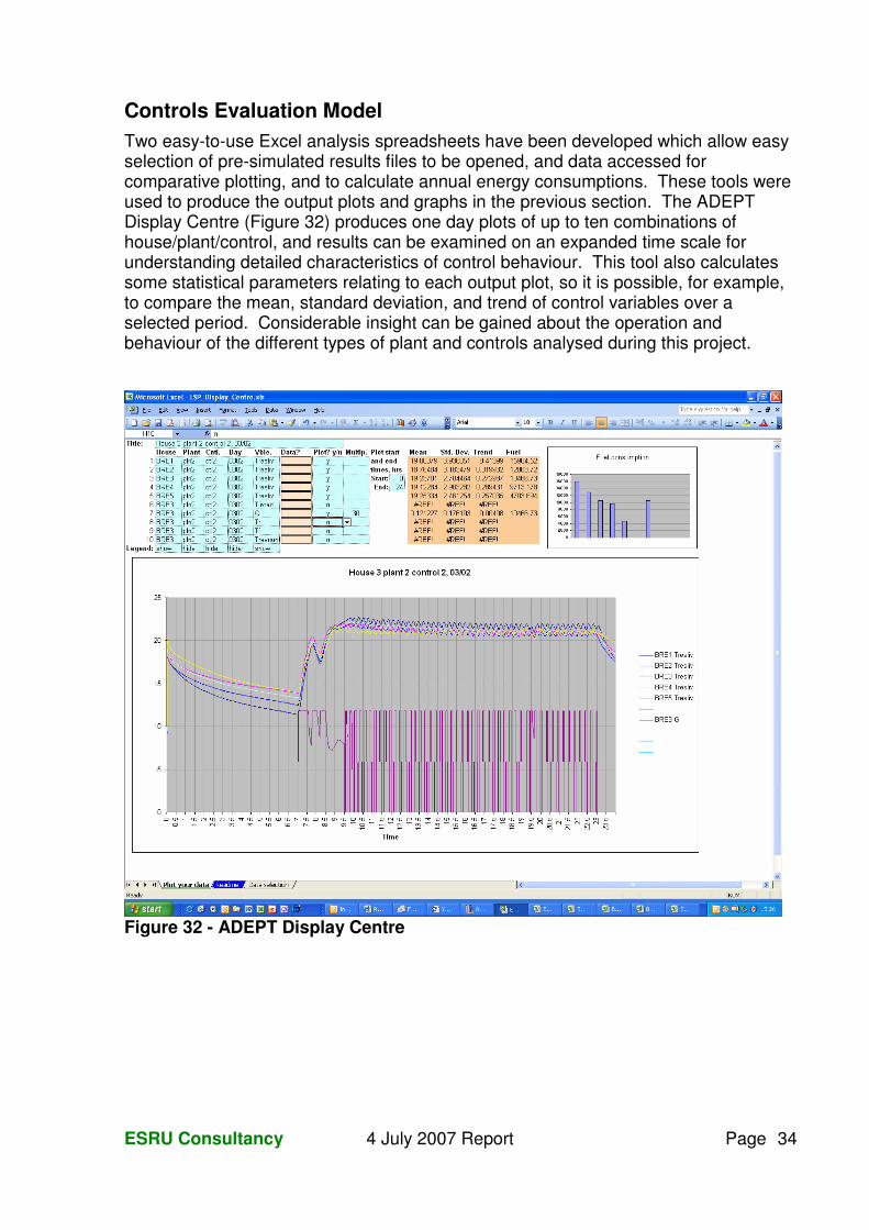
Controls Evaluation Model Two easy-to-use Excel analysis spreadsheets have been developed which allow easy selection of pre-simulated results files to be opened, and data accessed for comparative plotting, and to calculate annual energy consumptions. These tools were used to produce the output plots and graphs in the previous section. The ADEPT Display Centre (Figure 32) produces one day plots of up to ten combinations of house/plant/control, and results can be examined on an expanded time scale for understanding detailed characteristics of control behaviour. This tool also calculates some statistical parameters relating to each output plot, so it is possible, for example, to compare the mean, standard deviation, and trend of control variables over a selected period. Considerable insight can be gained about the operation and behaviour of the different types of plant and controls analysed during this project.
Figure 32 - ADEPT Display Centre
ESRU Consultancy 4 July 2007 Report Page 35
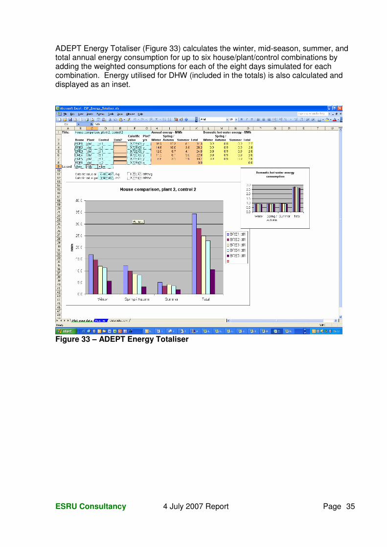
ADEPT Energy Totaliser (Figure 33) calculates the winter, mid-season, summer, and total annual energy consumption for up to six house/plant/control combinations by adding the weighted consumptions for each of the eight days simulated for each combination. Energy utilised for DHW (included in the totals) is also calculated and displayed as an inset.
Figure 33 – ADEPT Energy Totaliser
ESRU Consultancy 4 July 2007 Report Page 36
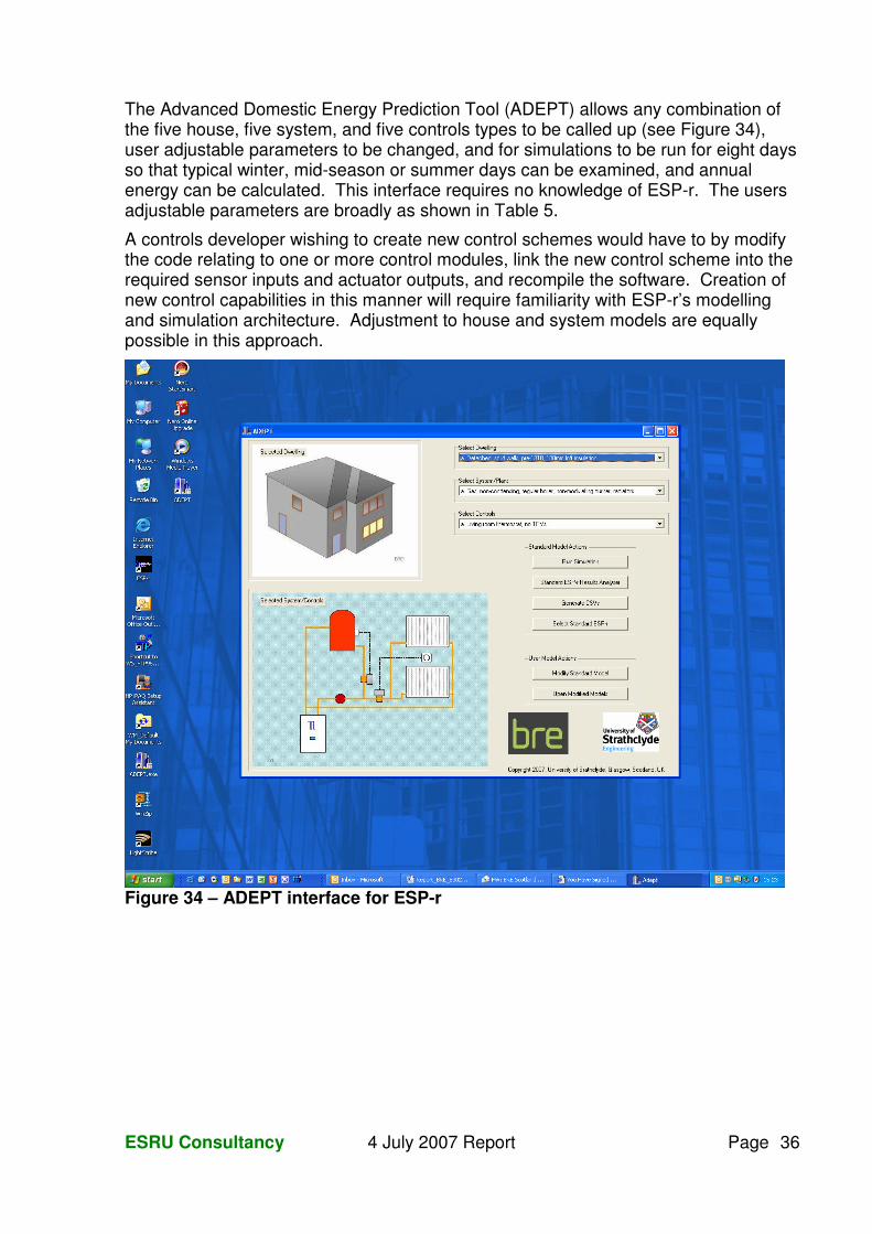
The Advanced Domestic Energy Prediction Tool (ADEPT) allows any combination of the five house, five system, and five controls types to be called up (see Figure 34), user adjustable parameters to be changed, and for simulations to be run for eight days so that typical winter, mid-season or summer days can be examined, and annual energy can be calculated. This interface requires no knowledge of ESP-r. The users adjustable parameters are broadly as shown in Table 5.
A controls developer wishing to create new control schemes would have to by modify the code relating to one or more control modules, link the new control scheme into the required sensor inputs and actuator outputs, and recompile the software. Creation of new control capabilities in this manner will require familiarity with ESP-r’s modelling and simulation architecture. Adjustment to house and system models are equally possible in this approach.
Figure 34 – ADEPT interface for ESP-r
ESRU Consultancy 4 July 2007 Report Page 37
SAP and BREDEM development This section contains:
• A summary of the parameters used to represent system controls in SAP / BREDEM and their impact on dwelling energy performance as calculated using SAP.
• SAP performance calculations for a selection of house/system/control combinations discussed in this report.
• Recommendations for future work.
The influence of controls on SAP / BREDEM calculations.
1-A. Hot water:
The water storage heat loss where it applies is dependent on controls.
Losses are multiplied by 1.3 if there is no cylinder stat (poor control).
Losses are multiplied by 0.9 if there is separate timer control of hot water and heating if both supplied from a common boiler system.
The water primary circuit heat loss (heat lost in primary circuit between boiler and water storage) where it applies is dependent on heating type and controls.
If a cylinder thermostat is installed, then losses are reduced by 250kWh/yr (insulated circuit) or 610 kWh/yr (un-insulated circuit).
In a combi boiler is installed, the losses due to water storage (if applicable) in a keep-hot facility are dependent on controls. If there is no time-clock then there is an additional 300kWh/yr loss.
1-B. Space heating:
Heating systems are characterised by their Efficiency, Heating type, and Responsiveness with further adjustments made based on control details.
1-B-1. Efficiencies:
Efficiencies come from the SEDBUK database or defaults are given in SAP tables. Note a very wide range of heating systems is considered from electric storage through heat pumps and CHP systems.
Efficiency adjustment for wet systems controls: boiler efficiency is adjusted down 5% if there is no room stat or boiler interlock and for condensing boilers the efficiency is adjusted up 2-3% if there is load compensation, weather compensation or under-floor heating.
Heat pump efficiencies are adjusted based on controls and whether DWH also supplied.
1-B-2. Heating type and responsiveness (living room temperature):
The heating type parameter is used in conjunction with the heat loss characteristics of the dwelling to establish the initial living room temperature. In very poorly insulated buildings with a heat loss parameter of around 6 W/m2(floor area).K the living room
ESRU Consultancy 4 July 2007 Report Page 38
temperature is around 1 degree lower than in well insulated buildings with a heat loss parameter of less than 1 W/m2(floor area).K. Similarly the non living areas are around 2 degrees lower for the poorly insulated building.
The responsiveness parameter is used to represent the ability of the heating system to adjust for gains or temperature fluctuations i.e. when there are gains then the heating controls should ideally adjust down the heat delivered by the heating system to maintain set-point if responsiveness is high. Where responsiveness is low then the system is less able to adjust and gains are not as effectively utilised; this is represented by an increase in internal temperatures (living and non living).
Examples of common heating types and responsiveness:
Old electric storage heaters are heating type 5, responsiveness of 0. Modern storage heaters are heating type 4, responsiveness of 0.25. Modern storage heaters with Celect control are heating type 2, responsiveness 0.75. Electric heat pumps are heating type 1, responsiveness of 1. Wet systems with radiators are heating type 1, responsiveness of 1. Wet systems with timber underfloor are heating type 1, responsiveness of 1. Wet systems with concrete underfloor are heating type 4, responsiveness of 0.25.
The internal living room temp of the property is then set based on the heating type and the building heat loss parameter. Type 1 living temps are around 18.6 deg, type 4 and 5 have living temps above 20deg (higher temps mean more heating degree days).
There is also an adjustment in the worksheet for the responsiveness of the system. More responsive systems have a reduction in living room temp.
1-B-3. Further Controls details (living room temp adjust, non living temperature):
Controls also influence the heating demands through adjustments to the living room temperatures and the difference between the living room and the non living space for the two zone model assumed in SAP.
Wet boiler systems with no controls are control type 1 and the living room temperature adjustment of +0.6deg applied.
Wet boiler systems with time and temperature zone controls are control type 3 and the living zone adjustment +0.0deg applied.
Further adjustments for controls can be made e.g. -0.15deg for a delayed start thermostat.
The temperature of the non living zone is set based on the control type and the buildings heat loss parameter. Controls type 1 has a smaller offset than type 3 and so the effect is that the non living area is a higher temperature in the type 1 case requiring more heating i.e. better controls mean a lower temperature is maintained in the non-living areas.
SAP calculations.
The following graphs and tables show the SAP calculation results across a range of the house types, system types and control options covered in this study.
ESRU Consultancy 4 July 2007 Report Page 39
Environmental Index(3 different house types, 4 different boilers, 2 control options)
0102030405060708090
100
roomstat roomstat roomstat roomstat roomstatplus trvs
roomstat roomstat roomstat roomstat roomstatplus trvs
roomstat roomstatplus trvs
65% effreg blr
75% effreg blr
82.5%reg blr
90% regcond blr
90% regcond blr
65% effreg blr
75% effreg blr
82.5%reg blr
90% regcond blr
90% regcond blr
90% regcond blr
90% regcond blr
pre-1919detached
pre-1919detached
pre-1919detached
pre-1919detached
pre-1919detached
UK avesemi
UK avesemi
UK avesemi
UK avesemi
UK avesemi
2007 midterr
2007 midterr
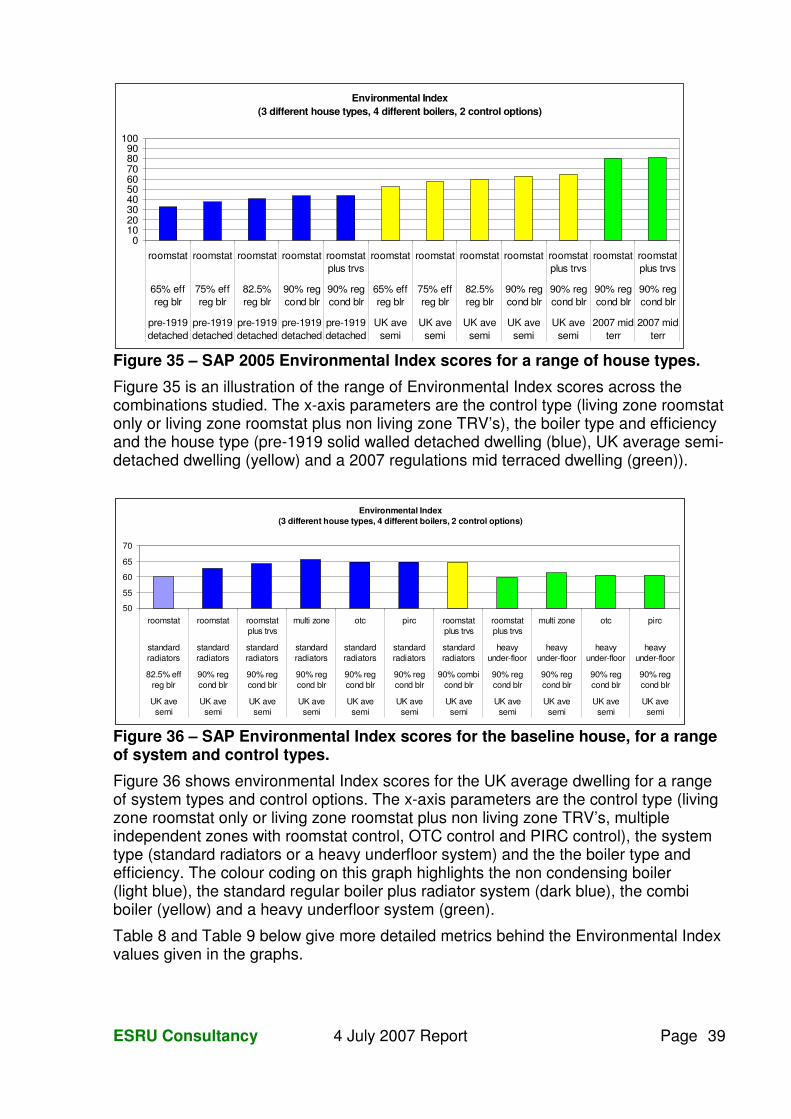
Figure 35 – SAP 2005 Environmental Index scores for a range of house types.
Figure 35 is an illustration of the range of Environmental Index scores across the combinations studied. The x-axis parameters are the control type (living zone roomstat only or living zone roomstat plus non living zone TRV’s), the boiler type and efficiency and the house type (pre-1919 solid walled detached dwelling (blue), UK average semi-detached dwelling (yellow) and a 2007 regulations mid terraced dwelling (green)).
Environmental Index
(3 different house types, 4 different boilers, 2 control options)
50
55
60
65
70
roomstat roomstat roomstatplus trvs
multi zone otc pirc roomstatplus trvs
roomstatplus trvs
multi zone otc pirc
standardradiators
standardradiators
standardradiators
standardradiators
standardradiators
standardradiators
standardradiators
heavyunder-floor
heavyunder-floor
heavyunder-floor
heavyunder-floor
82.5% effreg blr
90% regcond blr
90% regcond blr
90% regcond blr
90% regcond blr
90% regcond blr
90% combicond blr
90% regcond blr
90% regcond blr
90% regcond blr
90% regcond blr
UK avesemi
UK avesemi
UK avesemi
UK avesemi
UK avesemi
UK avesemi
UK avesemi
UK avesemi
UK avesemi
UK avesemi
UK avesemi
Figure 36 – SAP Environmental Index scores for the baseline house, for a range of system and control types.
Figure 36 shows environmental Index scores for the UK average dwelling for a range of system types and control options. The x-axis parameters are the control type (living zone roomstat only or living zone roomstat plus non living zone TRV’s, multiple independent zones with roomstat control, OTC control and PIRC control), the system type (standard radiators or a heavy underfloor system) and the the boiler type and efficiency. The colour coding on this graph highlights the non condensing boiler (light blue), the standard regular boiler plus radiator system (dark blue), the combi boiler (yellow) and a heavy underfloor system (green).
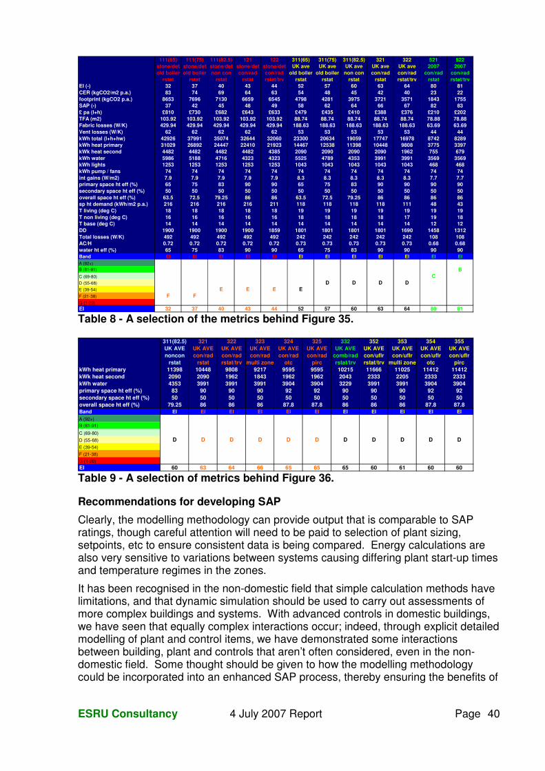
Table 8 and Table 9 below give more detailed metrics behind the Environmental Index values given in the graphs.
ESRU Consultancy 4 July 2007 Report Page 40
111(65) 111(75) 111(82.5) 121 122 311(65) 311(75) 311(82.5) 321 322 521 522stone/det stone/det stone/det stone/det stone/det UK ave UK ave UK ave UK ave UK ave 2007 2007old boiler old boiler non con con/rad con/rad old boiler old boiler non con con/rad con/rad con/rad con/rad
rstat rstat rstat rstat rstat/trv rstat rstat rstat rstat rstat/trv rstat rstat/trvEI (-) 32 37 40 43 44 52 57 60 63 64 80 81CER (kgCO2/m2 p.a.) 83 74 69 64 63 54 48 45 42 40 23 22footprint (kgCO2 p.a.) 8653 7696 7130 6659 6545 4798 4281 3975 3721 3571 1843 1755SAP (-) 37 42 45 48 49 58 62 64 66 67 82 83£ pa (l+h) £810 £730 £682 £643 £633 £479 £435 £410 £388 £376 £210 £202TFA (m2) 103.92 103.92 103.92 103.92 103.92 88.74 88.74 88.74 88.74 88.74 78.88 78.88Fabric losses (W/K) 429.94 429.94 429.94 429.94 429.94 188.63 188.63 188.63 188.63 188.63 63.69 63.69Vent losses (W/K) 62 62 62 62 62 53 53 53 53 53 44 44kWh total (l+h+hw) 42926 37991 35074 32644 32060 23300 20634 19059 17747 16978 8742 8289kWh heat primary 31029 26892 24447 22410 21923 14467 12538 11398 10448 9808 3775 3397kWk heat second 4482 4482 4482 4482 4385 2090 2090 2090 2090 1962 755 679kWh water 5986 5188 4716 4323 4323 5525 4789 4353 3991 3991 3569 3569kWh lights 1253 1253 1253 1253 1253 1043 1043 1043 1043 1043 468 468kWh pump / fans 74 74 74 74 74 74 74 74 74 74 74 74int gains (W/m2) 7.9 7.9 7.9 7.9 7.9 8.3 8.3 8.3 8.3 8.3 7.7 7.7primary space ht eff (%) 65 75 83 90 90 65 75 83 90 90 90 90secondary space ht eff (%) 50 50 50 50 50 50 50 50 50 50 50 50overall space ht eff (%) 63.5 72.5 79.25 86 86 63.5 72.5 79.25 86 86 86 86sp ht demand (kWh/m2 p.a.) 216 216 216 216 211 118 118 118 118 111 48 43T living (deg C) 18 18 18 18 18 19 19 19 19 19 19 19T non living (deg C) 16 16 16 16 16 18 18 18 18 17 19 18T base (deg C) 14 14 14 14 14 14 14 14 14 14 12 12DD 1900 1900 1900 1900 1859 1801 1801 1801 1801 1690 1458 1312Total losses (W/K) 492 492 492 492 492 242 242 242 242 242 108 108AC/H 0.72 0.72 0.72 0.72 0.72 0.73 0.73 0.73 0.73 0.73 0.68 0.68water ht eff (%) 65 75 83 90 90 65 75 83 90 90 90 90Band EI EI EI EI EI EI EI EI EI EI EI EIA (92+)B (81-91) BC (69-80) CD (55-68) D D D DE (39-54) E E E EF (21-38) F FG (1-20)EI 32 37 40 43 44 52 57 60 63 64 80 81 Table 8 - A selection of the metrics behind Figure 35.
311(82.5) 321 322 323 324 325 332 352 353 354 355UK AVE UK AVE UK AVE UK AVE UK AVE UK AVE UK AVE UK AVE UK AVE UK AVE UK AVEnoncon con/rad con/rad con/rad con/rad con/rad comb/rad con/uflr con/uflr con/uflr con/uflr
rstat rstat rstat/trv multi zone otc pirc rstat/trv rstat/trv multi zone otc pirckWh heat primary 11398 10448 9808 9217 9595 9595 10215 11666 11025 11412 11412kWk heat second 2090 2090 1962 1843 1962 1962 2043 2333 2205 2333 2333kWh water 4353 3991 3991 3991 3904 3904 3229 3991 3991 3904 3904primary space ht eff (%) 83 90 90 90 92 92 90 90 90 92 92secondary space ht eff (%) 50 50 50 50 50 50 50 50 50 50 50overall space ht eff (%) 79.25 86 86 86 87.8 87.8 86 86 86 87.8 87.8Band EI EI EI EI EI EI EI EI EI EI EIA (92+)B (81-91)
C (69-80)D (55-68) D D D D D D D D D D DE (39-54)F (21-38)G (1-20)EI 60 63 64 66 65 65 65 60 61 60 60 Table 9 - A selection of metrics behind Figure 36.
Recommendations for developing SAP
Clearly, the modelling methodology can provide output that is comparable to SAP ratings, though careful attention will need to be paid to selection of plant sizing, setpoints, etc to ensure consistent data is being compared. Energy calculations are also very sensitive to variations between systems causing differing plant start-up times and temperature regimes in the zones.
It has been recognised in the non-domestic field that simple calculation methods have limitations, and that dynamic simulation should be used to carry out assessments of more complex buildings and systems. With advanced controls in domestic buildings, we have seen that equally complex interactions occur; indeed, through explicit detailed modelling of plant and control items, we have demonstrated some interactions between building, plant and controls that aren’t often considered, even in the non-domestic field. Some thought should be given to how the modelling methodology could be incorporated into an enhanced SAP process, thereby ensuring the benefits of
ESRU Consultancy 4 July 2007 Report Page 41
more complex control systems, and any consequences of their interactions are correctly captured. The relationship between SBEM and dynamic simulation in the non-domestic field could be a model for future SAP and dynamic simulation in the domestic field.
Conclusion The objective of this project to produce a controls evaluation methodology based on computer modelling of domestic housing and heating systems has been achieved.
The evaluation methodology takes into account typical UK housing characteristics, climate, occupancy patterns, boiler, and heating system types, and uses the modelling tool ESP-r. Simulation time steps of one minute for the building and five seconds for the plant and controls was found to capture the short time constant dynamics associated with plant and controls. Additional output analysis tools allow easy selection of data for comparative plotting, and to calculate annual energy consumptions. Considerable insight can be gained about the operation and behaviour of the different types of plant and controls analysed during this project.
Control performance and energy consumptions is found to depend on many factors other than simply a particular system’s inherent efficiency. For example:
• A low rate of cool down overnight increases morning start-up energy requirement – favours less well insulated, lightweight constructions and heat emitters.
• OTC controls don’t maintain a precise room temperature setpoint, so their energy consumption will be sensitive to settings, and will vary throughout the year in comparison with room control systems.
• Comparison of systems with fixed on/off timer settings can be misleading, e.g. combi boiler systems will reach setpoint more rapidly than regular boiler systems, increasing their apparent energy consumption. In cold winter months, most systems don’t reach the setpoint temperature before the morning switch off time. This tends to favour less well insulated houses.
An interface has been developed that allows a user to select and modify parameters for the five house, system and control types, and to run ESP-r simulations for those adjusted configurations.
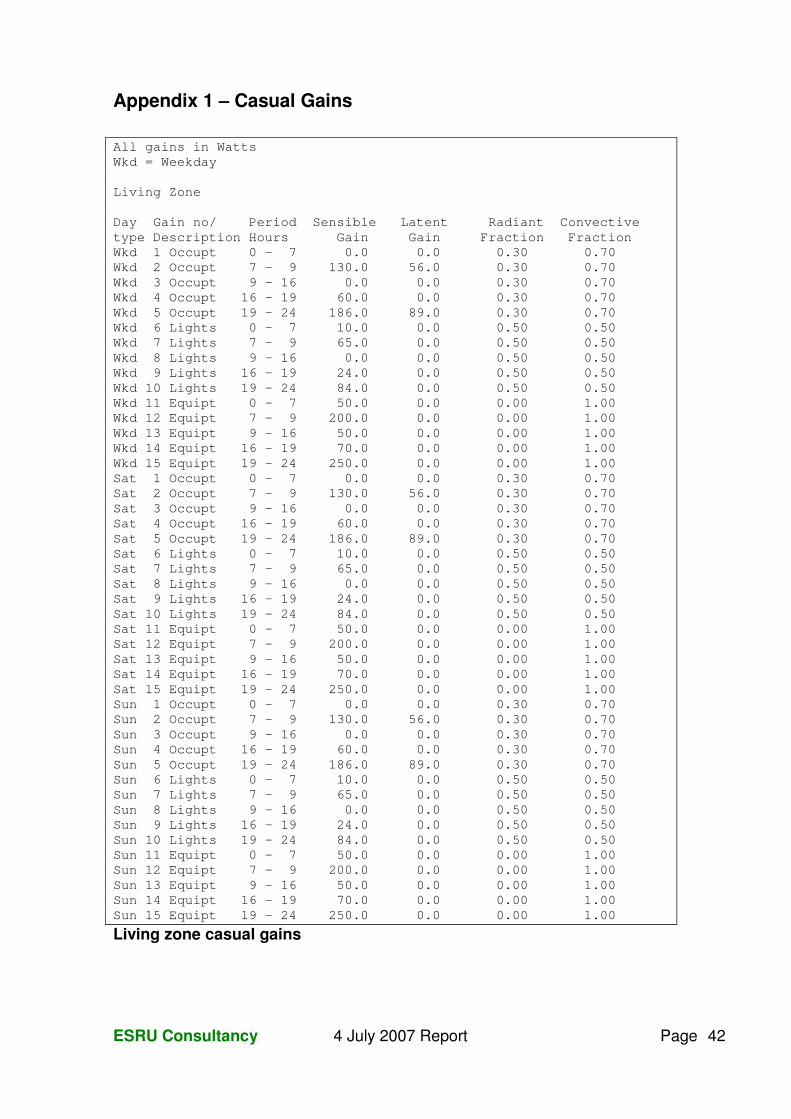
ESRU Consultancy 4 July 2007 Report Page 42
Appendix 1 – Casual Gains All gains in Watts Wkd = Weekday Living Zone Day Gain no/ Period Sensible Latent Radiant Convective type Description Hours Gain Gain Fraction Fraction Wkd 1 Occupt 0 - 7 0.0 0.0 0.30 0.70 Wkd 2 Occupt 7 - 9 130.0 56.0 0.30 0.70 Wkd 3 Occupt 9 - 16 0.0 0.0 0.30 0.70 Wkd 4 Occupt 16 - 19 60.0 0.0 0.30 0.70 Wkd 5 Occupt 19 - 24 186.0 89.0 0.30 0.70 Wkd 6 Lights 0 - 7 10.0 0.0 0.50 0.50 Wkd 7 Lights 7 - 9 65.0 0.0 0.50 0.50 Wkd 8 Lights 9 - 16 0.0 0.0 0.50 0.50 Wkd 9 Lights 16 - 19 24.0 0.0 0.50 0.50 Wkd 10 Lights 19 - 24 84.0 0.0 0.50 0.50 Wkd 11 Equipt 0 - 7 50.0 0.0 0.00 1.00 Wkd 12 Equipt 7 - 9 200.0 0.0 0.00 1.00 Wkd 13 Equipt 9 - 16 50.0 0.0 0.00 1.00 Wkd 14 Equipt 16 - 19 70.0 0.0 0.00 1.00 Wkd 15 Equipt 19 - 24 250.0 0.0 0.00 1.00 Sat 1 Occupt 0 - 7 0.0 0.0 0.30 0.70 Sat 2 Occupt 7 - 9 130.0 56.0 0.30 0.70 Sat 3 Occupt 9 - 16 0.0 0.0 0.30 0.70 Sat 4 Occupt 16 - 19 60.0 0.0 0.30 0.70 Sat 5 Occupt 19 - 24 186.0 89.0 0.30 0.70 Sat 6 Lights 0 - 7 10.0 0.0 0.50 0.50 Sat 7 Lights 7 - 9 65.0 0.0 0.50 0.50 Sat 8 Lights 9 - 16 0.0 0.0 0.50 0.50 Sat 9 Lights 16 - 19 24.0 0.0 0.50 0.50 Sat 10 Lights 19 - 24 84.0 0.0 0.50 0.50 Sat 11 Equipt 0 - 7 50.0 0.0 0.00 1.00 Sat 12 Equipt 7 - 9 200.0 0.0 0.00 1.00 Sat 13 Equipt 9 - 16 50.0 0.0 0.00 1.00 Sat 14 Equipt 16 - 19 70.0 0.0 0.00 1.00 Sat 15 Equipt 19 - 24 250.0 0.0 0.00 1.00 Sun 1 Occupt 0 - 7 0.0 0.0 0.30 0.70 Sun 2 Occupt 7 - 9 130.0 56.0 0.30 0.70 Sun 3 Occupt 9 - 16 0.0 0.0 0.30 0.70 Sun 4 Occupt 16 - 19 60.0 0.0 0.30 0.70 Sun 5 Occupt 19 - 24 186.0 89.0 0.30 0.70 Sun 6 Lights 0 - 7 10.0 0.0 0.50 0.50 Sun 7 Lights 7 - 9 65.0 0.0 0.50 0.50 Sun 8 Lights 9 - 16 0.0 0.0 0.50 0.50 Sun 9 Lights 16 - 19 24.0 0.0 0.50 0.50 Sun 10 Lights 19 - 24 84.0 0.0 0.50 0.50 Sun 11 Equipt 0 - 7 50.0 0.0 0.00 1.00 Sun 12 Equipt 7 - 9 200.0 0.0 0.00 1.00 Sun 13 Equipt 9 - 16 50.0 0.0 0.00 1.00 Sun 14 Equipt 16 - 19 70.0 0.0 0.00 1.00 Sun 15 Equipt 19 - 24 250.0 0.0 0.00 1.00
Living zone casual gains
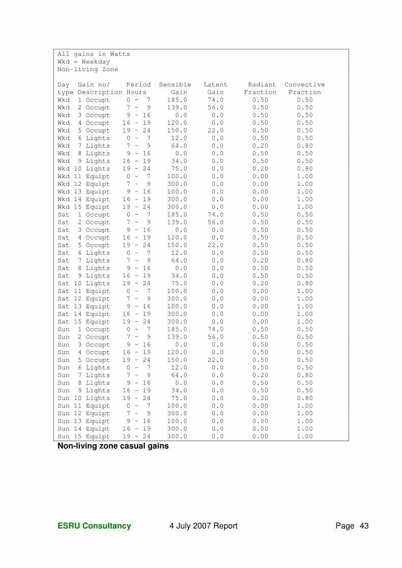
ESRU Consultancy 4 July 2007 Report Page 43
All gains in Watts Wkd = Weekday Non-living Zone Day Gain no/ Period Sensible Latent Radiant Convective type Description Hours Gain Gain Fraction Fraction Wkd 1 Occupt 0 - 7 185.0 74.0 0.50 0.50 Wkd 2 Occupt 7 - 9 139.0 56.0 0.50 0.50 Wkd 3 Occupt 9 - 16 0.0 0.0 0.50 0.50 Wkd 4 Occupt 16 - 19 120.0 0.0 0.50 0.50 Wkd 5 Occupt 19 - 24 150.0 22.0 0.50 0.50 Wkd 6 Lights 0 - 7 12.0 0.0 0.50 0.50 Wkd 7 Lights 7 - 9 64.0 0.0 0.20 0.80 Wkd 8 Lights 9 - 16 0.0 0.0 0.50 0.50 Wkd 9 Lights 16 - 19 34.0 0.0 0.50 0.50 Wkd 10 Lights 19 - 24 75.0 0.0 0.20 0.80 Wkd 11 Equipt 0 - 7 100.0 0.0 0.00 1.00 Wkd 12 Equipt 7 - 9 300.0 0.0 0.00 1.00 Wkd 13 Equipt 9 - 16 100.0 0.0 0.00 1.00 Wkd 14 Equipt 16 - 19 300.0 0.0 0.00 1.00 Wkd 15 Equipt 19 - 24 300.0 0.0 0.00 1.00 Sat 1 Occupt 0 - 7 185.0 74.0 0.50 0.50 Sat 2 Occupt 7 - 9 139.0 56.0 0.50 0.50 Sat 3 Occupt 9 - 16 0.0 0.0 0.50 0.50 Sat 4 Occupt 16 - 19 120.0 0.0 0.50 0.50 Sat 5 Occupt 19 - 24 150.0 22.0 0.50 0.50 Sat 6 Lights 0 - 7 12.0 0.0 0.50 0.50 Sat 7 Lights 7 - 9 64.0 0.0 0.20 0.80 Sat 8 Lights 9 - 16 0.0 0.0 0.50 0.50 Sat 9 Lights 16 - 19 34.0 0.0 0.50 0.50 Sat 10 Lights 19 - 24 75.0 0.0 0.20 0.80 Sat 11 Equipt 0 - 7 100.0 0.0 0.00 1.00 Sat 12 Equipt 7 - 9 300.0 0.0 0.00 1.00 Sat 13 Equipt 9 - 16 100.0 0.0 0.00 1.00 Sat 14 Equipt 16 - 19 300.0 0.0 0.00 1.00 Sat 15 Equipt 19 - 24 300.0 0.0 0.00 1.00 Sun 1 Occupt 0 - 7 185.0 74.0 0.50 0.50 Sun 2 Occupt 7 - 9 139.0 56.0 0.50 0.50 Sun 3 Occupt 9 - 16 0.0 0.0 0.50 0.50 Sun 4 Occupt 16 - 19 120.0 0.0 0.50 0.50 Sun 5 Occupt 19 - 24 150.0 22.0 0.50 0.50 Sun 6 Lights 0 - 7 12.0 0.0 0.50 0.50 Sun 7 Lights 7 - 9 64.0 0.0 0.20 0.80 Sun 8 Lights 9 - 16 0.0 0.0 0.50 0.50 Sun 9 Lights 16 - 19 34.0 0.0 0.50 0.50 Sun 10 Lights 19 - 24 75.0 0.0 0.20 0.80 Sun 11 Equipt 0 - 7 100.0 0.0 0.00 1.00 Sun 12 Equipt 7 - 9 300.0 0.0 0.00 1.00 Sun 13 Equipt 9 - 16 100.0 0.0 0.00 1.00 Sun 14 Equipt 16 - 19 300.0 0.0 0.00 1.00 Sun 15 Equipt 19 - 24 300.0 0.0 0.00 1.00
Non-living zone casual gains
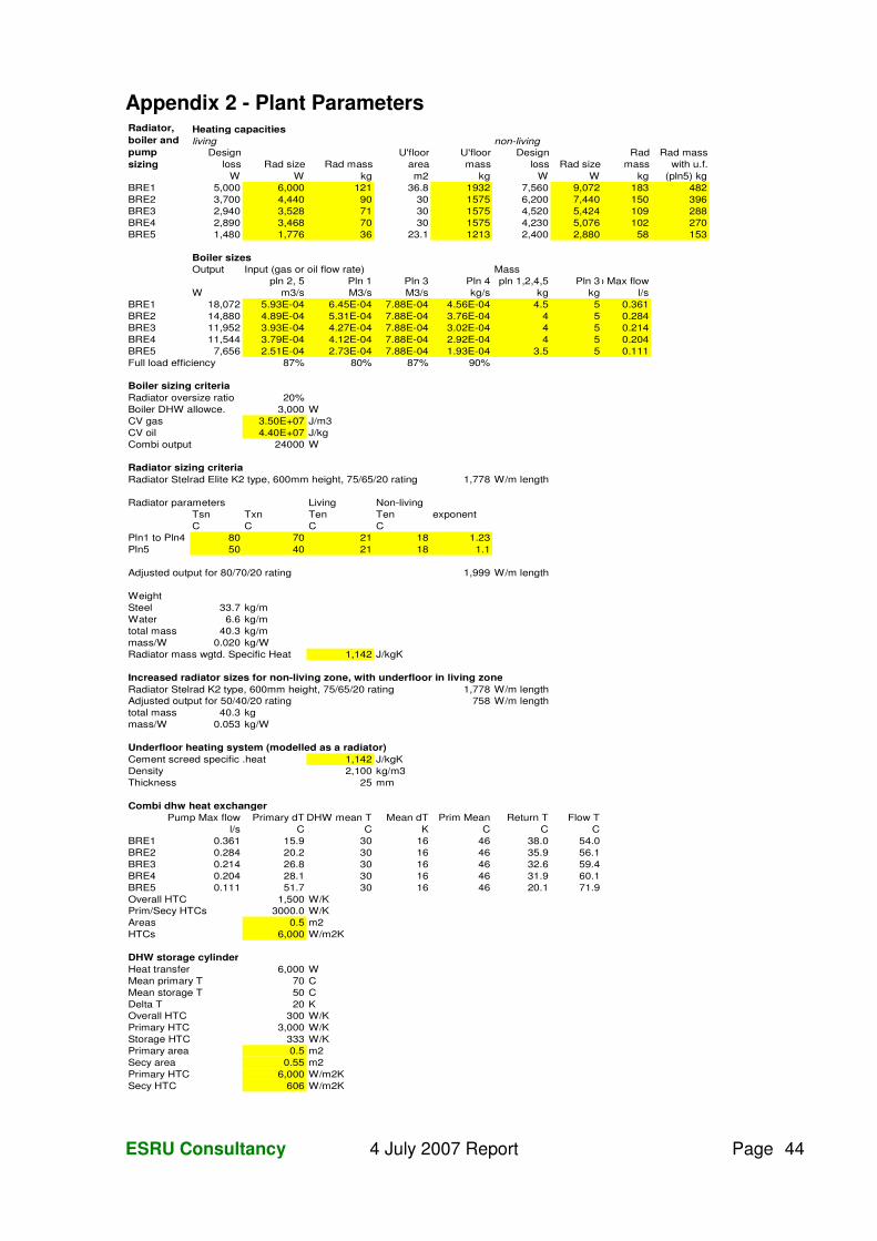
ESRU Consultancy 4 July 2007 Report Page 44
Appendix 2 - Plant Parameters Heating capacitiesliving non-living
Design loss Rad size Rad mass
U'floor area
U'floor mass
Design loss Rad size
Rad mass
Rad mass with u.f.
W W kg m2 kg W W kg (pln5) kgBRE1 5,000 6,000 121 36.8 1932 7,560 9,072 183 482BRE2 3,700 4,440 90 30 1575 6,200 7,440 150 396BRE3 2,940 3,528 71 30 1575 4,520 5,424 109 288BRE4 2,890 3,468 70 30 1575 4,230 5,076 102 270BRE5 1,480 1,776 36 23.1 1213 2,400 2,880 58 153
Boiler sizesOutput Input (gas or oil flow rate) Mass
pln 2, 5 Pln 1 Pln 3 Pln 4 pln 1,2,4,5 Pln 3Pump Max flowW m3/s M3/s M3/s kg/s kg kg l/s
BRE1 18,072 5.93E-04 6.45E-04 7.88E-04 4.56E-04 4.5 5 0.361BRE2 14,880 4.89E-04 5.31E-04 7.88E-04 3.76E-04 4 5 0.284BRE3 11,952 3.93E-04 4.27E-04 7.88E-04 3.02E-04 4 5 0.214BRE4 11,544 3.79E-04 4.12E-04 7.88E-04 2.92E-04 4 5 0.204BRE5 7,656 2.51E-04 2.73E-04 7.88E-04 1.93E-04 3.5 5 0.111Full load efficiency 87% 80% 87% 90%
Boiler sizing criteriaRadiator oversize ratio 20%Boiler DHW allowce. 3,000 WCV gas 3.50E+07 J/m3CV oil 4.40E+07 J/kgCombi output 24000 W
Radiator sizing criteriaRadiator Stelrad Elite K2 type, 600mm height, 75/65/20 rating 1,778 W/m length
Radiator parameters Living Non-livingTsn Txn Ten Ten exponentC C C C
Pln1 to Pln4 80 70 21 18 1.23Pln5 50 40 21 18 1.1
Adjusted output for 80/70/20 rating 1,999 W/m length
WeightSteel 33.7 kg/mWater 6.6 kg/mtotal mass 40.3 kg/mmass/W 0.020 kg/WRadiator mass wgtd. Specific Heat 1,142 J/kgK
Increased radiator sizes for non-living zone, with underfloor in living zoneRadiator Stelrad K2 type, 600mm height, 75/65/20 rating 1,778 W/m lengthAdjusted output for 50/40/20 rating 758 W/m lengthtotal mass 40.3 kgmass/W 0.053 kg/W
Underfloor heating system (modelled as a radiator)Cement screed specific .heat 1,142 J/kgKDensity 2,100 kg/m3Thickness 25 mm
Combi dhw heat exchangerPump Max flow Primary dT DHW mean T Mean dT Prim Mean Return T Flow T
l/s C C K C C CBRE1 0.361 15.9 30 16 46 38.0 54.0BRE2 0.284 20.2 30 16 46 35.9 56.1BRE3 0.214 26.8 30 16 46 32.6 59.4BRE4 0.204 28.1 30 16 46 31.9 60.1BRE5 0.111 51.7 30 16 46 20.1 71.9Overall HTC 1,500 W/KPrim/Secy HTCs 3000.0 W/KAreas 0.5 m2HTCs 6,000 W/m2K
DHW storage cylinderHeat transfer 6,000 WMean primary T 70 CMean storage T 50 CDelta T 20 KOverall HTC 300 W/KPrimary HTC 3,000 W/KStorage HTC 333 W/KPrimary area 0.5 m2Secy area 0.55 m2Primary HTC 6,000 W/m2KSecy HTC 606 W/m2K
Radiator, boiler and pump sizing