Report for Project 6: Survival Analysis

Bohai Zhang, Shuai Chen

Data description: This dataset is about the survival time of German patients with various facial cancers which contains 762 patients’ records. The following is a summary about the original data set:

ID: Patient’s identification number Anfang: First date the patient was diagnosed with cancer

Ende The date the patient died or the last day the patient was seen alive Data_diff Ende minus Anfang, the unit is by days Interval Time period between Anfang and Ende (by days)

Tod Indicator variable, Tod=1 if the patient died; Tod=0, if data is censored value

T Tumor size, it has 4 levels from 1 to 4 in an increasing order N Node attack, it has 4 levels in an increasing order M Metastasis, it is measured as 0 and 1

Stadium Stage of Cancer, it has 4 levels in an increasing order Status Status spread or not and it has 3 levels LOK Location of the tumor in the oral cavity with 5 levels P53 A protein which regulates the cell cycle with 3 levels RB A protein which regulates the cell cycle with 2 levels

BCL2 Protein BCL2 which is a cell signaling protein with 5 levels P16 A protein which regulates the cell cycle with 3 levels.

MDM2 A protein regulator for protein P53 with 5 levels. C-MYC A know oncogenic gene with 4 levels CK-14 A subtype of low weight Cytokeratins with five levels HPV Human Papilloma Virus with 3 levels.

The data are right censored. All 14 covariates are discrete factors with several levels. Our goal is to estimate survival function with respect to the 14 variables. Furthermore, we can find the relationship between covariates and patients’ survival function. There are some missing data. 95 records do not have the time period between the first visit and last visit or indicator of death. Thus, we discard these records and the left dataset have 667 records.

Part1: Kaplan-Meier estimator for survival function. We have the Kaplan-Meier estimator of survival function:

Where ds = number of failures at time ts and Ns = number of alive just before time ts. Kaplan-Meier estimator is nonparametric, which requires no parametric assumptions. We can compare data from two different groups by visual inspection of their respective estimated survival functions or some statistical tests. Thus, we can compare different levels of a certain factor.

1. 1 Kaplan-Meier estimator of the entire data set. The K-M estimator for the entire data is as follows:

records events median 0.95LCL 0.95UCL

667 335 1250 1035 1915 Here the median of failure time is defined as the time at which survival function is 0.5. To compare KM estimator with other two naive methods, we can compare this estimated median of failure time: Naive method 1 (consider all data as dead at the last visit): The median is 778. Naive method 2 (only use the uncensored data): The median is 423. As KM estimator is unbiased and thus its median can be viewed as near to true value. We can find both the two naïve methods underestimate the true median, and even smaller than the lower limit given by KM estimator.

1.2 Compare survival functions on different levels by KM estimator. There are 14 factors in the dataset and we will consider one factor each time. For each level of a factor, KM estimator will only use the data which are on this level. Thus, if the data size for one level is too small to get a good estimator, we can consider combining it with other levels. There are many missing data for some factors. We do not delete these incomplete data now, because their information may be useful for other factors. For the data with missing levels, we ascribe them to a new level ‘Unknown’. If the level ‘Unknown’ has a small data size (<5), we just randomly distribute a level to this observation. To decide the importance of a factor, we use log-rank test (generalized Mantel-Haenszel statistic), which tests whether there is difference between survival curves of different levels. The main idea of log-rank test is to construct a table at each distinct death time, and compare the observed and expected death rates between the groups. (H0: no difference between groups) Here are KM plots for each factor: (1) T: The tumor size. This factor has 4 levels from 1 to 4 in an increasing order of tumor size. We find there is only one record with T=0, so combine this level with T=1. For the missing levels, we ascribe them to a new level ‘Unknown’. The log-rank test shows difference is significant, p-value= 2.11e-15. The K-M estimator with T is as follows:

(2) N: Node attack. It has 4 levels from 0-3 in an increasing order. After observing this factor, we see there are only 3 data with N=5, so combine it with level ‘3’. For missing data, we ascribe them to an ‘unknown’ level. The plot of K-M estimator with N is as follows:

The further log-rank test shows difference is significant, the p-value= 0

(3) M: Metastasis. It has two levels 0 and 1. After observing data, we find there is one record with M=2 and one record with M=5 and we combine them to the ‘Unknown’ level.

The further log-rank test shows difference is significant, the p-value = 1.35e-07 (4) Stadium: stage of cancer. The factor stadium has 4 levels from 1 to 4 in an increasing order. From the graph, we can see the survive probability for stage3 is bigger than that of stage2, which is a bit surprising. The further log-rank test shows difference is significant. P-value=1.11e-15.

(5) Status: the status spread or not. It has 3 levels from 1 to 3.

We notice that level 1 and level 2 are very similar so we combine it as the factor 1&2. The number of missing data is only two, so randomly distribute them to other levels. The above graph is the K-M estimator with status factor before and after this data manipulation. Log-rank test shows difference is significant (P-value= 0.000594). (6) LOK: location of tumor in the oral cavity. This factor has 5 levels and no missing data.

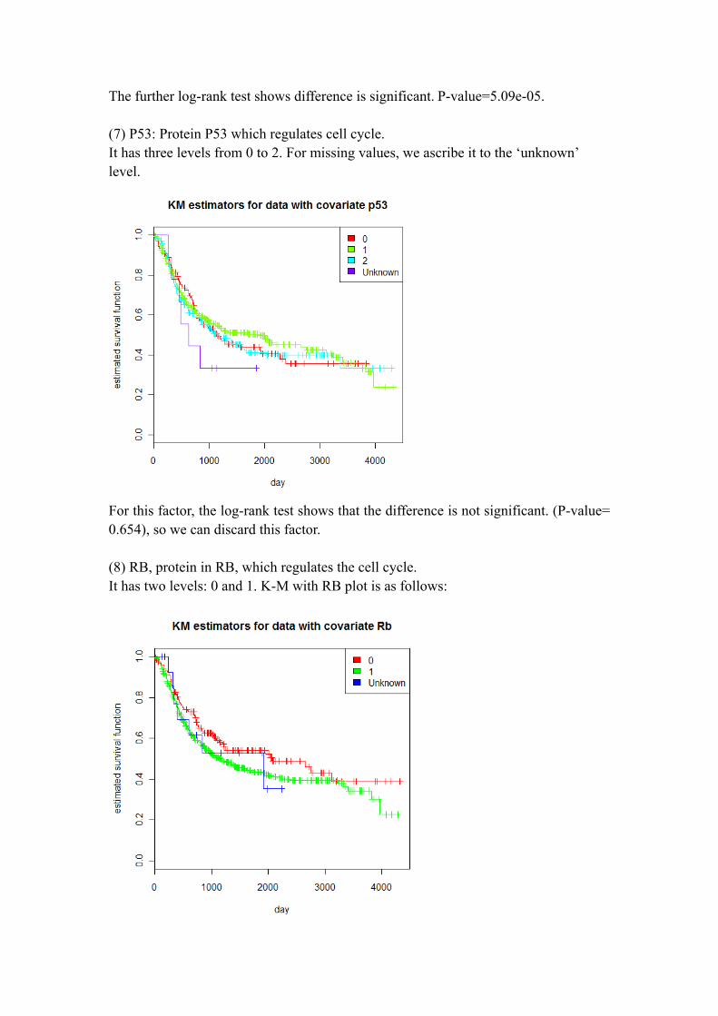
The further log-rank test shows difference is significant. P-value=5.09e-05. (7) P53: Protein P53 which regulates cell cycle. It has three levels from 0 to 2. For missing values, we ascribe it to the ‘unknown’ level.

For this factor, the log-rank test shows that the difference is not significant. (P-value= 0.654), so we can discard this factor. (8) RB, protein in RB, which regulates the cell cycle. It has two levels: 0 and 1. K-M with RB plot is as follows:

Further log-rank test shows that the difference is not significant (p-value= 0.165), so we can discard this factor. (9) BCL2: one kind of protein. This factor has5 levels from 0 to 4. From the original K-M plot, we find the level 1&2 and level 3&4 are very similar, so we combine 1&2 and 3&4 as one factor respectively. Then the K-M plot with covariate BCL2 is as follows:

By further log-rank test, the p-value=0.00473, so the difference is significant. (10) P16, protein p16 which regulates the cell cycle. It has 3 levels from 0 to 2. The plot of K-M estimator with this covariate is as follows:

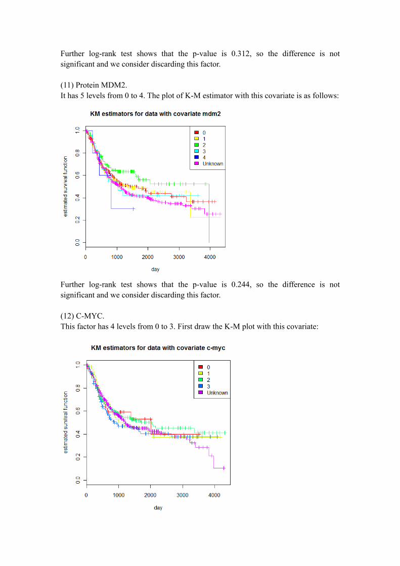
Further log-rank test shows that the p-value is 0.312, so the difference is not significant and we consider discarding this factor. (11) Protein MDM2. It has 5 levels from 0 to 4. The plot of K-M estimator with this covariate is as follows:

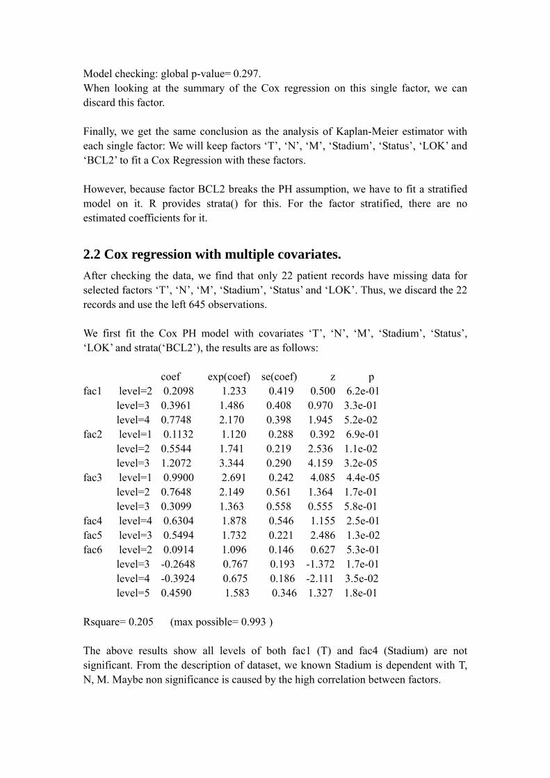
Further log-rank test shows that the p-value is 0.244, so the difference is not significant and we consider discarding this factor. (12) C-MYC. This factor has 4 levels from 0 to 3. First draw the K-M plot with this covariate:

We can see the curves of the 4 levels are very similar. Further log-rank test shows that the p-value is 0.801, so the difference is not significant. (13) CK-14. This factor has 5 known levels from 0 to 5. The missing data accounts for a large proportion, about 51.72%. The plot of K-M estimator with this factor is as follows:

The further log-rank test shows that the p-value is 0.137, so the difference is not significant and we will discard this factor. (14). HPV score, Human Papilloma Virus. It has 3 known levels, from 0 to 2. The missing data account for 83.2% and we ascribe them to the ‘Unknown’ level. The K-M estimator with HPV is as follows:

The log-rank test shows that the p-value is 0.539, so the difference is not significant. After the above analysis, we find factors ‘T’, ‘N’, ‘M’, ‘Stadium’, ‘Status’, ‘LOK’ and ‘BCL2’ (7 factors) make contribution to survival of patients.

Part2: COX Proportional Hazards Regression KM estimator cannot cope with complicated model with several factors or continuous covariates. However, Cox PH model can be used to model complicated structures. Cox PH model assumes proportional hazard:

h(t)=h0(t)exp(βTx) Where h0(t) is unspecified and called baseline hazard function. Because baseline is estimated non-parametrically, this is a semi-parametric model. R provides function coxph() to fit the model. Here all variables are factors, so R will automatically set dummy variables for each factor. In default, R will delete first level to achieve identifiability. Thus, the values of x in the hazard function are all 0 or 1. If estimated coefficient β>0, this level will increase the hazard of patients, comparing with the 1st level, which means patients on this level face more risk than patients on the first level. We check the proportional hazard assumption by function cox.zph() provided by R, main idea of which is to check the residuals with a suitable transformation of time. If the p-value is smaller than 0.05 for a factor, Cox regression may not proper. To solve this problem, we can divide the data into strata based on this factor. Each stratum is permitted to have a different baseline hazard function, while the coefficients of the remaining covariates are assumed to be constant across strata.

2.1 Single factor. We first fit Cox Regression with single factor to compare with KM estimator: (1) Factor T. Model checking: global p-value=0.823; Summary of Cox regression:

regressor coef exp(coef) se(coef) P-value fac12 0.8839 2.4204 0.2712 0.001119 fac13 0.9291 2.5323 0.2783 0.000841 Fac14 1.6252 5.0796 0.2537 1.49e-10

fac1Unknown 1.3567 3.8834 0.4125 0.001005

Every coefficient is significant nonzero. The p-value of Likelihood ratio test is 3.331e-16; The p-value of Wald test is 9.87e-14; The p-value of Score (log rank) test is p=2.109e-15.

(2) Factor N. Model checking: global p-value=0.3195 Summary of Cox regression:

regressor coef exp(coef) se(coef) P-value Fac21 0.2369 1.2673 0.2438 0.3312 Fac22 0.9524 2.5919 0.1376 4.46e-12 Fac23 1.6968 5.4564 0.2187 8.55e-15

Fac2Unknown 0.8453 2.3286 0.3539 0.0169 The likelihood ration test, Wald test and score test have p-value close to 0. So keep this factor.

(3) Factor M.

Model checking: global p-value= 0.1135 Summary of Cox regression:

regressor coef exp(coef) se(coef) P-value

Fac31 1.1536 3.1695 0.2219 2.01e-07 Fac3Unknown 0.4456 1.5615 0.2946 0.13 All the three tests have p-values very close to zero, so keep it. (4) Stadium.

Model checking: global p-value= 0.762 Summary of Cox regression:

regressor coef exp(coef) se(coef) P-value Fac42 0.9631 2.6199 0.3686 0.008975 Fac43 0.5693 1.767 0.3844 0.138571 Fac44 1.7621 5.8249 0.3223 4.58e-08

Fac4Unknown 1.6355 5.1319 0.4598 0.000375 All the three tests have p-values close to 0. So keep it. (5) Status. Model checking: fac53’s p-value= 0.72 Summary of Cox regression:

regressor coef exp(coef) se(coef) P-value Fac53 0.7143 2.0427 0.2124 0.00077

Likelihood ratio test, Wald test and Score test all have very small p-value. So keep it. (6) Factor LOK.

Model checking: global p-value=0.3827

Summary of Cox regression:

regressor coef exp(coef) se(coef) P-value Fac42 0.1754 1.1917 0.1382 0.204466 Fac43 -0.6123 0.5421 0.1743 0.000442 Fac44 0.0584 1.0601 0.1645 0.722636

Fac4Unknown 0.3345 1.3973 0.3336 0.316048 All the three tests have p-values close to 0. So keep it. (7) Factor P53. The plot of Cox-PH model with P53 estimator for survival function is as follows:

Model checking: global p-value= 0.528. Summary of Cox regression:

regressor coef exp(coef) se(coef) P-value Fac71 -0.06671 0.93547 0.15122 0.659 Fac72 0.02997 1.03042 0.16433 0.855

Fac7Unknown 0.38153 1.46452 0.42898 0.374 So, all the coefficients are not significant nonzero. The p-value of likelihood ratio test is 0.6835, the p-value of the Wald test is 0.6574 and the p-value of the score test is 0.654. So we will discard this variable.

(8) RB Model checking: global p-value=0.728 All the coefficients are not significant nonzero and the likelihood ratio test, Wald test and score test have large P-value. So discard this covariate.

(9) BCL2.

Model checking: global p-value= 0.03064 Summary of Cox regression:

regressor coef exp(coef) se(coef) P-value Fac91 -0.5402 0.5826 0.1618 0.000839 Fac93 -0.3369 0.7140 0.2006 0.093090

Fac9Unknown -0.1386 0.8706 0.1864 0.457267 Likelihood ratio test: p=0.003126 Wald test: p=0.005337 Score (log rank) test: p=0.00474 The results show this factor should be kept. However, the model assumption checking indicates this factor break the proportional hazard assumption. (10) P16. Model checking: global p-value=0.0504 For this factor, all the coefficients are not significant nonzero and the likelihood ratio test, Wald test and score test have large P-value. So discard this covariate. The following is the plot of Cox-PH model with P16 for survival function:

(11) Mdm2. Model checking: global p-value=0.860 All the coefficients are not significant nonzero and the likelihood ratio test, Wald test and score test have large P-value. So discard this covariate.

(12) C-MYC Model checking: global p-value=0.118 All the coefficients are not significant nonzero and the likelihood ratio test, Wald test and score test have large P-value. So discard this covariate.

(13) CK-14.

Model checking: global p-value=0.0401 The three tests show no significant difference, so we discard it. (14) HPV score.

Model checking: global p-value= 0.297. When looking at the summary of the Cox regression on this single factor, we can discard this factor. Finally, we get the same conclusion as the analysis of Kaplan-Meier estimator with each single factor: We will keep factors ‘T’, ‘N’, ‘M’, ‘Stadium’, ‘Status’, ‘LOK’ and ‘BCL2’ to fit a Cox Regression with these factors. However, because factor BCL2 breaks the PH assumption, we have to fit a stratified model on it. R provides strata() for this. For the factor stratified, there are no estimated coefficients for it.

2.2 Cox regression with multiple covariates. After checking the data, we find that only 22 patient records have missing data for selected factors ‘T’, ‘N’, ‘M’, ‘Stadium’, ‘Status’ and ‘LOK’. Thus, we discard the 22 records and use the left 645 observations. We first fit the Cox PH model with covariates ‘T’, ‘N’, ‘M’, ‘Stadium’, ‘Status’, ‘LOK’ and strata(‘BCL2’), the results are as follows: coef exp(coef) se(coef) z p fac1 level=2 0.2098 1.233 0.419 0.500 6.2e-01

level=3 0.3961 1.486 0.408 0.970 3.3e-01 level=4 0.7748 2.170 0.398 1.945 5.2e-02

fac2 level=1 0.1132 1.120 0.288 0.392 6.9e-01 level=2 0.5544 1.741 0.219 2.536 1.1e-02 level=3 1.2072 3.344 0.290 4.159 3.2e-05

fac3 level=1 0.9900 2.691 0.242 4.085 4.4e-05 level=2 0.7648 2.149 0.561 1.364 1.7e-01 level=3 0.3099 1.363 0.558 0.555 5.8e-01

fac4 level=4 0.6304 1.878 0.546 1.155 2.5e-01 fac5 level=3 0.5494 1.732 0.221 2.486 1.3e-02 fac6 level=2 0.0914 1.096 0.146 0.627 5.3e-01

level=3 -0.2648 0.767 0.193 -1.372 1.7e-01 level=4 -0.3924 0.675 0.186 -2.111 3.5e-02 level=5 0.4590 1.583 0.346 1.327 1.8e-01

Rsquare= 0.205 (max possible= 0.993 ) The above results show all levels of both fac1 (T) and fac4 (Stadium) are not significant. From the description of dataset, we known Stadium is dependent with T, N, M. Maybe non significance is caused by the high correlation between factors.

Thus, we try to discard fac4 (Stadium) and refit the model with covariates ‘T’, ‘N’, ‘M’, ‘Status’ ,‘LOK’ and strata(‘BCL2’), the results are as follows: coef exp(coef) se(coef) z p fac1 level=2 0.6673 1.949 0.278 2.4008 1.6e-02

level=3 0.7171 2.048 0.291 2.4636 1.4e-02 level=4 1.1827 3.263 0.272 4.3415 1.4e-05

fac2 level=1 0.0151 1.015 0.251 0.0601 9.5e-01 level=2 0.6042 1.830 0.165 3.6544 2.6e-04 level=3 1.2322 3.429 0.257 4.7915 1.7e-06

fac3 level=1 1.0006 2.720 0.238 4.1973 2.7e-05 fac5 level=3 0.5571 1.746 0.221 2.5245 1.2e-02 fac6 level=2 0.1090 1.115 0.145 0.7508 4.5e-01

level=3 -0.2665 0.766 0.193 -1.3843 1.7e-01 level=4 -0.3698 0.691 0.185 -2.0006 4.5e-02 level=5 0.5545 1.741 0.340 1.6286 1.0e-01

Rsquare= 0.201 (max possible= 0.993 ) Now all factors are significant and p-values of remained factors are smaller than before. Rsquare= 0.201 means the variation is explained by these factors by 20%. The coefficients of fac1 (T) are increasing by levels, meaning the larger tumor size brings higher risk, which is the same with our intuition. Similar conclusions can be made for other factors. Then we check the PH assumption again: rho chisq p fac102 0.0330 0.3572 0.5501 fac103 0.0734 1.6202 0.2031 fac104 0.0691 1.5091 0.2193 fac201 -0.0947 2.9408 0.0864 fac202 -0.0410 0.5912 0.4420 fac203 -0.0655 1.5546 0.2125 fac301 0.0506 0.9279 0.3354 fac503 -0.0235 0.1836 0.6683 fac602 -0.0106 0.0376 0.8463 fac603 -0.0451 0.7092 0.3997 fac604 -0.0512 0.9086 0.3405 fac605 -0.0601 1.1795 0.2775 GLOBAL NA 8.9229 0.7095 All p-values are above 0.05, and the global p-value is 0.7095, which means it is proper to use this Cox PH model to draw some conclusions.