report - ntnufolk.ntnu.no/andersty/4. klasse/tkp4170 - prosjektering... · norwegian university of...

NTNU Faculty of Natural Sciences and Technology Norwegian University of Department of Chemical Engineering Science and Technology

REPORT

TKP4170 – Process Desing, Project

Title: Coal Plant Svalbard (TEMP)

Location: Trondheim, Norway

Date: November 17, 2013

Authours:

Aqeel Hussain

Reza Farzad

Anders Leirpoll

Kasper Linnestad

Supervisor: Sigurd Skogestad

Number of pages:

Report:

Appendices:

Abstract

I hereby declare that the work is performed in compliance with the

exam regulations of NTNU.

Date and signatures

-

TKP4170 [Type the document title]

i

Table of Contents 1 Introduction to Coal-Fired Power Plants 1

1.1 Conventional Coal-Fired Power Plants 1

1.1.1 Supercritical Coal Fired Power Plants 2

1.2 Integrated Gasification Combined Cycle Coal-Fired Power Plants 3

1.3 Oxygen-Fired Coal Combustion Power Plants (Chemical Looping Combustion) 3

2 Introduction to Flue Gas Treatment 4

2.1 CO2 Capture 4

2.1.1 Post-Combustion Capture 4

2.1.2 Pre-Combustion Capture 5

2.1.3 Oxygen-Fired Combustion 6

2.1.4 Carbon Storage 6

2.1.5 Economics of Capture 7

2.2 Flue Gas Desulphurization 8

2.2.1 Wet scrubbing 8

2.2.2 Dry Scrubbing 9

2.3 NOx Removal 10

3 Design Basis 10

4 Process Descriptions 11

4.1 Current Plant at Svalbard 11

4.1.1 Boiler 11

4.1.2 Steam Cycle 11

4.1.3 District Heating 11

4.1.4 Gas Treatment 12

4.2 Proposed Pulverized Coal plant with Carbon Capture and Storage 12

4.2.1 Pulverized Coal Boiler 12


4.2.3 Flue Gas Treatment 13

4.2.4 District Heating 13

4.3 Case Studies 13

4.3.1 District heating Case 13

4.3.2 Heat Pump Case 13

5 Flowsheet Calculations 13

5.1 District Heating Case 13

5.1.1 Flow diagram 14

ii

5.1.2 Stream Data 14

5.1.3 Compositions 15

5.1.4 Boiler Temperature 17

5.1.5 Steam Cycle Pressure 17

5.2 Heat Pump Case 18

5.2.1 Flow Diagram 18

5.2.2 Stream Data 18

5.2.3 Compositions 19

5.2.4 Coefficient of performance 20

6 Cost Estimation 20

6.1 Capital Costs of Major Equipment 20

6.1.1 Pulverized Coal boiler 20

6.1.2 Heat exchangers 21

6.1.3 Turbines 21

6.1.4 Compressors 21

6.1.5 Pumps 22

6.1.6 Flue Gas Desulfurization 22

6.1.7 Carbon Capture 22

6.1.8 Heat Pump Costs 22

6.1.9 Total Equipment Costs 22

6.2 Variable Costs 24

6.2.1 Labor 24

6.2.2 Diesel Costs 24

6.2.3 Cost of Coal 24

6.2.4 Operation and Maintenance 25

6.2.5 Chemicals 25

6.2.6 Total Variable Costs 25

6.3 Revenues 25

6.4 Working Capital 25

7 Investment Analysis 25

7.1 District Heating Case 26

7.2 Heat Pump Case 26

8 Discussion 27

8.1 Plant Choices 27

8.1.1 Plant Type 27

iii


8.1.3 Flue Gas Treatment 28

8.2 Case Studies 28

8.2.1 District Heating Case 28

8.2.2 Boiler Temperature 29

8.2.3 Steam Cycle Pressure 29

8.2.4 Heat Pump Case 29

8.3 Investments 29

Mangler 29

9 Conclusion and Recommendations 29

References 29

Appendix A - Cost estimation for the district heating case A-1

A.1 Major A-1

Appendix B - Cost estimation for the heat pump case B-1

1

1 Introduction to Coal-Fired Power Plants For more than 100 years, coal-fired power plants have generated the major portion of the

worldwide electric power [1] with a current (2011) market supply share of 41.2% [2]. Coal is

the largest growing source of primary energy worldwide, despite the decline in demand among

the E D countries, due to hina’s high increase in demand [3]. The Chinese coal consumption

and production account for more than 45% of both global totals, and it has been estimated that

their share will pass 50% by 2014 because of their high demand for cheap energy [3]. This will

drastically increase the world total -production which will contribute greatly to the global

warming and other environmental effects such as ocean acidification [4]. It will therefore be of

great importance to develop clean and efficient coal plants which can produce electricity that

can compete with the prices of the cheap, polluting coal plants that currently exists. Some

instances of such plants have been proposed as alternatives to the conventional coal-fired power

plant and they will be given an introduction in this report.

1.1 Conventional Coal-Fired Power Plants Conventional coal-fired power plants use pulverized coal (PC) or crushed coal and air as a fuel to

the furnace. The coal is pulverized by crushing and fed to the reactor at ambient pressures and

temperatures and burned in excess of air. The excess of air is introduced to lower the furnace

temperature which makes the equipment cheaper as it does not have to withstand extreme

temperatures, and it also reduces the formation of . is formed at high temperatures and

is a pollutant that has a negative effect on the health of humans besides contributing to acidic

precipitation [5]. The hot flue gas from the furnace is used to heat up the boiler which produces

high pressure (HP) steam. This steam is in turn expanded in a turbine arrangement that

generate electrical power. The low pressure (LP) steam is then condensed and re-fed to the

boiler. The hot flue gas contains pollutants and aerosols which have to be removed before the

gas is vented through the stack to the atmosphere. Pollutants that have to be removed include

mercury, and . The nitrous oxides are usually removed using selective catalytic

reduction (SCR) where ammonia is used as a reducing agent [6]. The sulfur, mercury and other

solid matter is normally removed as solid matter by reducing the sulfurous oxide using lime and

water, and then passing the flue gas through an electrostatic precipitator or a fabric filter. The

slurry is then collected for safe deposition. Conventional coal plants operating using subcritical

(sC) conditions, which will result in low overall plant efficiency [7]. A conceptual process flow

diagram of this power plant is shown in Figure 1.1.

2

Figure 1.1: Simplified process flow diagram for the conventional coal plant. Where HRSG is the heat recovery steam generator and FGT is the flue gas treatment (desulfurization, mercury removal, dust removal etc.)

1.1.1 Supercritical Coal Fired Power Plants

The efficiency of the plant can be increase by using supercritical (SC) steam conditions with

higher pressure. The plant efficiency is increasing both for increasing pressure drop and

increasing temperature. There is therefore a constant development of better equipment that can

withstand higher steam pressures and temperatures [7]. Some examples of conditions are listed

in Table 1.1. The ultra supercritical configuration is currently under development and is

expected to be available in 2015 [7]. A typical heat recovery steam generator design is shown in

Figure 1.2.

Figure 1.2: Heat recovery steam generator cycle with three pressure levels, HP, IP and LP. Where HP is high pressure, IP I intermediate pressure and LP is low pressure. Table 1.1: Some typical HP steam conditions [7]

Temperature

Pressure [bar]

Depleted < 500 < 115 Subcritical (sC) 500-600 115-170

Boiler

FGT

HRSG

Coal

Air

To CO2-

extraction

Ash

Power

HP IP LP

Condenser

District heating

3

Temperature

Pressure [bar]

Supercritical (SC) 500-600 230-265 Ultra supercritical ~730 ~345

1.2 Integrated Gasification Combined Cycle Coal-Fired Power Plants Integrated gasification combined cycle power plants feed compressed oxygen and slurry of coal

and water to a gasifier. The gasifier converts the fuel to synthesis gas (syngas) which is then

treated to remove sulfur, mercury and aerosols. The syngas is then brought to a combustor with

compressed air diluted with nitrogen in a turbine. The flue gas is then used to create steam by

passing it through a heat recovery steam generator (HRSG). This steam is passed through a

series of turbines, as with the conventional plant. The efficiency gain this method has compared

to the conventional plant is that the combustor turbine operates at a very high temperature

(~1500 ), but it also has to have an air separation unit (ASU) to achieve reasonable conversion

rates for the gasification process [8]. The integrated gasification combined cycle (IGCC) power

plants require large investments because of all the advanced utilities such as a fluidized bed

reactor for gasification and an air separation unit. The IGCC power plants can achieve up to 3%

higher efficiencies which can be worth the investment in the long run, especially for huge power

plants [7].

Figure 1.3: Simplified process flow diagram for the IGCC power plant. Where HRSG is the heat recovery steam generator, FGT is the flue gas treatment (desulfurization, mercury removal, dust removal etc.) and ASU is the air separation unit.

1.3 Oxygen-Fired Coal Combustion Power Plants (Chemical Looping

Combustion) Oxygen-fired coal combustion power plants, also known as chemical looping combustion, burn

PC with pure oxygen which creates a flue gas that has a very high carbon dioxide concentration.

This has the advantage that the flue gas can be injected directly into storage after

Fluidized bed gasifier FGT

Coal

Air HRSG Power

ASU

Water

Oxygen

Ash

Slurry

Power

To CO2-

extraction

Nitrogen

4

desulfurization, and cleaning. This technology is currently under development and several pilot

plants have been built [9]. Unlike the other power plant designs, this design does not suffer a

significant loss in efficiency when carbon capture and storage (CCS) is implemented. For a

conventional power plant the loss in efficiency can be up to 14%, while the oxygen-fired power

plant only suffers losses of around 3% [7] [10]. Another advantage is that there will not be any

formation of nitrous oxides due to the lack of nitrogen in the feed, however the concentration of

sulfur oxide will increase due to the flue gas recycle. This is on the other hand not seen as a

major problem as sulfur oxide can be treated by introducing lime in the reactor.

Figure 1.4: Simplified process flow diagram for the oxygen-fired coal combustion power plant. Where HRSG is the heat recovery steam generator, FGT is the flue gas treatment (desulfurization, mercury removal, dust removal etc.) and ASU is the air separation unit.

2 Introduction to Flue Gas Treatment

2.1 CO2 Capture Energy supply from fossil fuels is associated with large emissions of and account for 75% of

the total emissions. emissions will have be to cut down by 50% to 85% to achieve the

goal of restricting average global temperature increase to the range of to [4]. Industry

and power generation have the potential to reduce the emission of greenhouse gases by 19% by

2050, by applying carbon capture and storage [11]. There are three basic systems for

capture.

Post-combustion capture

Pre-combustion capture

Oxygen fuelled combustion capture

2.1.1 Post-Combustion Capture

CO2 captured from flue gases produced by combustion of fossil fuel or biomass and air is

commonly referred to as post-combustion. The flue gases are passed through a separator where

is separated from the flue gases. There are several technologies available for post-

combustion carbon capture from the flue gases, usually by using a solvent or membrane. The

process that looks most promising with current technologies is the absorption process based on


Coal

Air HRSG Power

ASU

Water

Oxygen

Ash

Slurry

To CO2-

injection

Nitrogen

5

amine solvents. It has relatively high capture efficiency, high selectivity of and lowest energy

use and cost in comparison with other technologies. In absorption processes is captured

using the reversible nature of chemical reactions of an aqueous alkali solution, usually an amine,

with carbon dioxide. After cooling the flue gas it is brought into contact with solvent in an

absorber at temperatures of to . The regeneration of solvent is carried out by heating

in a stripper at elevated temperatures of to . This requires a lot of heat from the

process, and is the main reason why capture is expensive [12].

Membrane processes are used for capture at high pressure and higher concentration of

carbon dioxide. Therefore, membrane processes require compression of the flue gases; as a

consequence this is not a feasible solution with available technology as of 2013. However, if the

combustion is carried out under high pressure, as with the IGCC process, membranes can

become a viable option once they achieve high separation of [13].

Figure 2.1: Conceptual process flow diagram of the absorption process. Here HEX is the heat-exchanger used to minimize the total heat needed for separation of carbon dioxide.

2.1.2 Pre-Combustion Capture

Pre combustion involves reacting fuel with oxygen or air, and converting the carbonaceous

material into synthesis gas containing carbon monoxide and hydrogen. During the conversion of

fuel into synthesis gas, CO2 is produced via water-shift reaction. CO2 is then separated from the

synthesis gas using a chemical or physical absorption process resulting in H2 rich fuel which can

be further combusted with air. Pressure swing adsorption is commonly used for the purification

of syngas to high purity of H2, however, it does not selectively separate CO2 from the waste gas,

which requires further purification of CO2 for storage. The chemical absorption process is also

used to capture CO2 from syngas at partial pressure below 1.5 MPa. The solvent removes CO2

from the shifted syngas by mean of chemical reaction which can be reversed by high pressure

and heating. The physical absorption process is applicable in gas streams which have higher CO2

Absorption Regenerator

Flue gas

HEX

Clean flue gas

Rich absorbent

Lean absorbent

Absorbent make-up

CO2 for

injection

Re-boiler

6

partial pressure or total pressure and also with higher sulfur contents. This process is used for

the capturing of both H2S and CO2, and one commercial solvent is Selexol [7].

Figure 2.2: Schematic drawing of an integrated gasification combined cycle plant with pre-combustion carbon caption. The carbon monoxide from the gasifier is converted to carbon dioxide and hydrogen by reacting it with steam in the shift reactor. The carbon dioxide is captured in the carbon capture unit (CC, see Figure 2.1), and pure hydrogen is burned with nitrogen diluted air.

2.1.3 Oxygen-Fired Combustion

In oxy fuel combustion, oxygen is separated in an air separation unit and sent to a combustor for

combustion of fuel. Recycled CO2-rich flue gas is added to keep the temperature low; otherwise

the material of construction would be compromised. Combustion takes place in a mixture of

O2/CO2, and the resulting flue gas has a high CO2.purity. The flue gas is almost free of nitrogen-

gases and after removal of sulfur the flue gas is 90 % CO2, rest H2O. There is no need of further

CO2-capture, and the CO2 can be compressed and stored [10].

2.1.4 Carbon Storage

After the carbon dioxide has been compressed it can be injected into storage. is usually

stored in geological formation at depths of 1000 m or more [14]. Hence high pressures are

required before injection, which has the advantage that can be injected as a supercritical

fluid. This will reduce the pipeline diameter and, consequently capital cost [15]. The oil industry

is experienced on the geological difficulties, and may be able to provide expertise on the

geological formation and how they will react to carbon dioxide injection. The storage site and

reservoir has to be closely monitored to ensure that the carbon dioxide does not escape into the

atmosphere or nearby drinking water supplies. With careful design of injection and appropriate

monitoring of well pressure and local -concentrations, it can be ensured that the injected

carbon dioxide remains underground for thousands of years [14].


Coal

Air HRSG Power

ASU

Water

Oxygen

Ash

Slurry

Power

To atmosphere

Shift reac-

tor

To CO2-

injection

CC

Steam

7

2.1.5 Economics of Capture

CO2 capture is an expensive process both in capital costs and variable costs. Post combustion

absorption by amine solution can add as high as a 14% energy penalty even with state of the art

CO2 capture technology [7]. The capital costs depend highly on the flow rate of flue gas, as this

increases the regenerator and compressor size. The variable costs are also increased with higher

flue gas flow, as more sorbent is required, and the cost of CO2-transport and storage will

increase [16]. Improving process configurations and solvent capacity can majorly reduce power

demand for the regenerator. Such improvements include: absorber intercooling, stripper

interheating, flashing systems and multi-pressure stripping, though all of these will come at the

expense of complexity and higher capital costs. Table 2.1 shows the development in MEA

absorption systems from year 2001 to 2006 [17].

Table 2.1: Economics of CO2 capture by MEA scrubbing [17].

Year of design 2001 2006

MEA [weight percent] 20 30 Power used [MWh/ton] 0.51 0.37 @ $ 80/MWh [$/ton CO2 removed] 41 29 Capital cost [$/ton CO2 removed per year] 186 106 @ 16%/year [$/ton CO2 removed] 30 17 Operating and maintenance cost [$/ton CO2 removed] 6 6 Total cost [$/ton CO2 removed] 77 52 Net CO2 removal with power replaced by gas [%] 72 74

The enviromental impact is commonly expressed as cost per pollutant removed or cost per

pollutant avoided. Cost of CO2 per tom removed is different from cost of CO2 avoided and cost of

CO2 avoided is given as [18] :

cost o a oided ( tonne⁄ ) ( h⁄ ) ( h⁄ )

(tonne h⁄ ) (tonne h⁄ ) (1)

Table 2.2 shows the cost variability and representative cost values for power generation and CO2

capture, for the three fuel systems respectively. The cost of electricity is lowest for the NGCC,

regardless of CO2 capture. Pulverized Coal plant has lower capital cost without capture while

IGCC plant has lower cost when current CO2 capture is added in the system.

Table 2.2: Summary of reported CO2 emissions and costs for a new electric power plant with and without CO2 capture base don current technology (excluding CO2 transport and storage costs). Here MWref is the reference plant net output, COE is the cost of electricity, Rep. value is the representative value, PC means pulverized coal plant, NGCC means natural gas combined cycle plant and IGCC = integrated gasification combined cycle coal plant [19].

Cost and Performance Measures

PC Plant IGCC Plant NGCC Plant

Range low-high

Rep. value

Range low-high

Rep. value

Range low-high

Rep. value

Emission rate w/o capture [kg CO2/MWh]

722-941 795 682-846 757 344-364

358

Emission rate with capture [kg CO2/MWh]

59-148 116 70-152 113 40-63 50

Percent CO2 reduction per kWh [%]

80-93 85 81-91 85 83-88 87

Capital cost w/o capture [$/kW]

1100-1490

1260 1170-1590

1380 447-690

560

8

Cost and Performance Measures

PC Plant IGCC Plant NGCC Plant

Range low-high

Rep. value

Range low-high

Rep. value

Range low-high

Rep. value

Capital cost with capture [$/kW]

1940-2580

2210 1410-2380

1880 820-2020

1190

Percent increase in capital cost [%]

67-87 77 19-66 36 37-190 110

COE w/o capture [$/MWh] 37-52 45 41-58 48 22-35 31 COE with capture [$/MWh] 64-87 77 54-81 65 32-58 46 Percent increase in COE w/capture [%]

61-84 73 20-55 35 32-69 48

Cost of CO2 avoided [$/t CO2] 42-55 47 13-37 26 35-74 47 Cost of CO2 captured [$/t CO2] 29-44 34 11-32 22 28-57 41 Energy penalty for capture [% MWref]

22-29 27 12-20 16 14-16 15

2.2 Flue Gas Desulphurization SO2 has a harmful effect both on humans and the environment. Exposure to higher

concentrations of SO2 is the cause of many harmful diseases. SO2 affects the environment by

reacting into acids and is a major source of acid rain [20]. Combustion of sulfur-containing

compounds such as coal is therefore a major source of SO2 generation. Removal of sulfur from

solid fuels is not practical, so the sulfur is removed from the flue gas after combustion of coal.

The removal of sulfur oxide from the flue gasses is achieved by physical or chemical absorption

process [21]. There are two commonly used industrial processes for the desulphurization of flue

gasses [22], wet and dry scrubbing.

2.2.1 Wet scrubbing

In wet scrubbing, a solvent is used for the absorption of SO2. Typically water is considered to be

the cheapest sol ent It’s washing capacity howe er is ery limited and huge quantity o water

has to be used. Approximately 75 tons of water is used per ton of flue gas, and even then 5% of

SO2 remains [21].

In advanced processes, flue gas is treated with an alkaline slurry in an absorber, where SO2 is

captured, shown in Figure 2.3. The most commonly used slurry is composed of limestone, which

reacts with the sulfur. The sulfur removal efficiency is 98 % for wet scrubbing process. Carbon

dioxide removal units include a polishing scrubber which lowers flue gas SO2 content from 44

ppmv to 10 ppmv [7].

9

Figure 2.3: Flue gas desulfurization via wet scrubbing using limestone slurry. NEEDS SOURCE! XX ??

Wet scrubbing process is mostly used with higher sulfur contents with economic efficiency of 95

to 98%. The main disadvantage of wet scrubbing is acidic environment which can be corrosive.

Therefore, corrosion resistant material is required for the construction which increases capital

cost of the plant. The other disadvantage includes consumption of large quantity of water for the

process.

2.2.2 Dry Scrubbing

Dry scrubbing is useful for coal with lower sulfur content. It also has the major advantage of

maintaining a higher temperature of the emission gasses, while wet scrubbing decreases the

temperature to that of water used [20]. Lime is normally used as sorbent-agent during the dry

scrubbing process. The dry sorbent reacts with the flue gas at 1 to remove SO2. In dry

scrubbing adiabatic saturation approach is normally applied. Adiabatic saturation is required to

achieve high SO2 removal, thereby carefully controlling the amount of water [20].

Figure 2.4: Flue gas desulfurization via dry scrubbing using limestone. NEEDS SOURCE! XX ??

Relatively poor utilization of reagent is the main disadvantage of dry sorbent process, which

increases the operational costs. Dry scrubbing uses a minimal amount of water, and leaves the

flue gas dry, reducing risk of corrosion. Relatively dry calcium sulfite is obtained as by-product

with fly ash [20].

10

2.3 NOx Removal Selective catalystic reduction (SCR) approach is applied for removal of NOx, where the flue gas is

reduced with ammonia over a catalyst to nitrogen and water. The SCR has a efficiency of 80 to 90

% for NOx removal. The optimal temperature range is , with vanadium and titanium

as catalyst, and the following reaction is carried out during the process:

(2)

Ammonia is either injected in pure form under pressure or in an aqueous solution. Instead of

ammonia, urea can also be used for the process. The main challenge of the process is full

conversion as emission of the NH3 is highly undesirable. The unreacted NH3 can also oxidize SO2

to SO3 that further react with NH3 to form ammonium bisulfate. Ammonium bisulfate is a sticky

solid material which can plug the downstream equipment. The catalyst activity is very critical

with SCR because catalyst can costs up to of the capital cost [6].

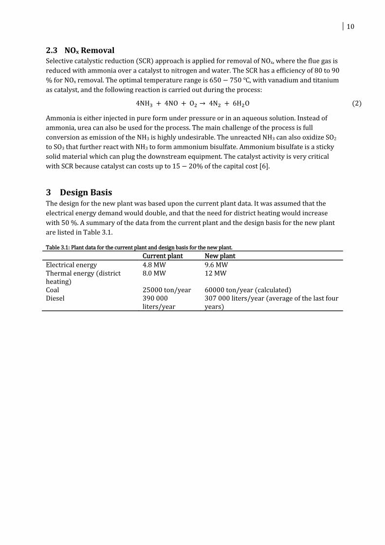
3 Design Basis The design for the new plant was based upon the current plant data. It was assumed that the

electrical energy demand would double, and that the need for district heating would increase

with 50 %. A summary of the data from the current plant and the design basis for the new plant

are listed in Table 3.1.

Table 3.1: Plant data for the current plant and design basis for the new plant.

Current plant New plant

Electrical energy 4.8 MW 9.6 MW Thermal energy (district heating)

8.0 MW 12 MW

Coal 25000 ton/year 60000 ton/year (calculated) Diesel 390 000

liters/year 307 000 liters/year (average of the last four years)

11

4 Process Descriptions

4.1 Current Plant at Svalbard

Figure 4.1: Process flow diagram of current plant at Svalbard

4.1.1 Boiler

Coal is crushed and fed to the boiler along with air, where it combusts at high temperatures

forming flue gas and ash. The air is blown into the boiler by fans. Water is circulated through the

evaporator-drums in the boiler to yield pressurized steam. The flue gas is sent directly to the

stack and out to the atmosphere.

4.1.2 Steam Cycle

The hot steam from the boiler is split into two streams, one of which is sent to a condensing

steam turbine, the other to a backpressure steam turbine. The steam from the condensing steam

turbine is quenched in a condenser that is cooled with seawater; this allows the outlet pressure

from the turbine to be relatively low, depending on how much it is cooled. The backpressure

steam turbine has a relatively high back pressure, which yields moderately high temperatures in

the outlet stream. This heat is exploited by heating up cold water from the district heating

network. The two different streams are then combined, sent through a pump and back to the

boiler.

4.1.3 District Heating

The district heating water circulates Longyearbyen, and is used to heat houses and tap water,

before it is sent back to the power plant for reheating. The water is pumped to a heat exchanger

where it is reheated by the condensing steam from the back pressure steam turbine. After which

it is sent back to the district heating network.

Boiler

District heating

Coal

Air

Ash Main Water

Pump

Sea water Pump

Sea water

Condenser Condensing

Steam Turbine

District Heat Water Pump

Flue Gas Back Pressure Steam Turbine

12

4.1.4 Gas Treatment

The flue gas is currently not treated before it is sent trough the stack to the atmosphere.

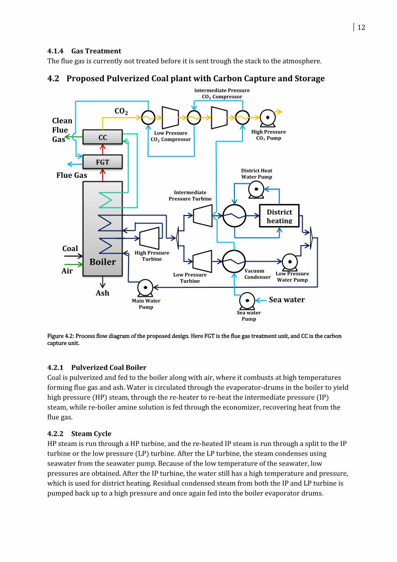
4.2 Proposed Pulverized Coal plant with Carbon Capture and Storage

Figure 4.2: Process flow diagram of the proposed design. Here FGT is the flue gas treatment unit, and CC is the carbon capture unit.

4.2.1 Pulverized Coal Boiler

Coal is pulverized and fed to the boiler along with air, where it combusts at high temperatures

forming flue gas and ash. Water is circulated through the evaporator-drums in the boiler to yield

high pressure (HP) steam, through the re-heater to re-heat the intermediate pressure (IP)

steam, while re-boiler amine solution is fed through the economizer, recovering heat from the

flue gas.

4.2.2 Steam Cycle

HP steam is run through a HP turbine, and the re-heated IP steam is run through a split to the IP

turbine or the low pressure (LP) turbine. After the LP turbine, the steam condenses using

seawater from the seawater pump. Because of the low temperature of the seawater, low

pressures are obtained. After the IP turbine, the water still has a high temperature and pressure,

which is used for district heating. Residual condensed steam from both the IP and LP turbine is

pumped back up to a high pressure and once again fed into the boiler evaporator drums.

Boiler

District heating

FGT

CC

Coal

Air

Ash Main Water

Pump Sea water

Pump

Sea water

Vacuum Condenser Low Pressure

Turbine Low Pressure Water Pump

Intermediate Pressure Turbine

High Pressure Turbine

District Heat Water Pump

Low Pressure 𝐂𝐎𝟐 Compressor

intermediate Pressure 𝐂𝐎𝟐 Compressor

High Pressure 𝐂𝐎𝟐 Pump

Clean

Flue Gas

Flue Gas

𝐂𝐎𝟐

13

4.2.3 Flue Gas Treatment

The flue gas out of the boiler is first desulfurized in the flue gas desulfurization unit (FGD), using

a seawater scrubber. The seawater is used to cool steam and CO2 earlier in the process, and then

fed to the seawater scrubber. As the concentration of sulfur in the water out is low, it can safely

be pumped back to the ocean. As the flue gas is quenched through seawater, dust patricles and

mercury is also removed.

After FGD, the flue gas goes through carbon capture (CC) using an amine solution. CO2-free flue

gas is sent out to the environment, while the captured CO2 is sent to compression and storage.

Here the CO2 is cooled with seawater and compressed two times, before being pumped as a

supercritical fluid down into geological formations.

4.2.4 District Heating

The proposed pulverized coal power plant will use the same district heating network as is

already built on Svalbard, giving a steam split-factor between IP and LP turbines. The district

heating water circulates Longyearbyen, and is used to heat houses and tap water. After being

used, the water is sent back to the power plant. The cycle introduces a pressure drop, which is

equalized by the district heating water pump.

4.3 Case Studies In the report two different cases will be studied, one using the existing district heating loop on

Svalbard, another introducing a central heat pump.

4.3.1 District heating Case

The district heating case uses the current district heating network on Svalbard, and produces 12

MW of district heating, with double the current electric power, giving 9.6 MW of electric energy.

The split of steam to IP turbine for district heating and LP turbine for pure electric generation is

adjustable, and was adjusted to fit the design basis (REF ?? TABLE DESIGN BASIS), using as little

coal as possible.

4.3.2 Heat Pump Case

The heat pump case is an attempt at maximizing electric energy produced, to use the electric

energy in heat pumps instead of district heating. This model has the possibility of selling excess

electric power to the neighboring town of Barentsburg, but is highly dependent on good

coefficient of performance for the heat pump. Investment analysis is performed on both cases,

using the same amount of coal, to compare them to eachother.

5 Flowsheet Calculations

5.1 District Heating Case The plant is modeled using Aspen Y Y , based on the results rom the report “ ost and

Per ormance Baseline or Fossil Energy Plants” by the ational Energy Technology Laboratory

[7]. The simplifications and assumptions that are made are listed below.

The coal is assumed to be pure carbon with the same net calorific value as the coal on

Svalbard.

The boiler is modeled as a combustion reactor with a maximum temperature of ,

followed by a heat exchanger.

14

The boiler is assumed to combust the coal completely.

The boiler is assumed to have a minimum temperature approach of , this is obtained

by adjusting the flow of water in the steam cycle.

The flue gas desulfurization is not included in the model.

The carbon capture is modeled as a pure component splitter with a given heat

requirement for re-boiling the rich amine solution in the stripper column.

The HP steam temperature and pressure are set to and 165 bar respectively.

The outlet pressure of the HP steam turbine is set to 49 bar, and is reheated to .

The vacuum pressure created by the condenser is set to 0.01 bar.

The seawater is assumed to be .

The district heating network is modeled as heat exchangers with an inlet temperature of

, an outlet temperature of and a pressure drop of 5 bar. This is obtained by

adjusting the flow of water in the district heating network.

The compressor train for the compression of carbon dioxide for storage is modeled as

two compressors and a pump with intercooling using heat exchanger with cold seawater.

The inter-stage pressures for the CO compressor train are found by trial and error to

yield the lowest amount of work needed.

The adiabatic efficiencies of all the compressors and pumps are assumed to be .

The split ratio between the LP steam turbine and the IP steam turbine are chosen to

yield a total district heating of 12 MW.

The amount of air blown into the boiler is chosen to yield a maximum combustion

temperature of 800 .

The amount of heat needed to the reboiler to the stripper is based on a 90% CO capture,

and an amount of heat needed per kilo CO removed ( k

kg CO ).

5.1.1 Flow diagram

The process flow diagram from the Aspen HYSYS model is shown in Figure 5.1.

Figure 5.1: The process flow diagram from the Aspen HYSYS model for the district heating case.

5.1.2 Stream Data

The important stream data for the different streams in the Aspen HYSYS model are shown in

Table 5.1.

Table 5.1: Stream data for the district heating case, calculated in Aspen HYSYS.

Stream name Vapour fraction

Temperature [ ]

Pressure [bar]

Mass flow [ton/year]

Air 1.00 10.00 1.0 2.22E+06

15


Temperature [ ]

Pressure [bar]


Coal 0.00 10.00 1.0 6.00E+04

Flue gas 1.00 799.99 1.0 2.28E+06

Slurry 0.00 799.99 1.0 0.00E+00

1 0.00 40.36 3.0 2.86E+05

2 0.00 41.30 165.0 2.86E+05

3 1.00 600.00 165.0 2.86E+05

4 1.00 407.07 49.0 2.86E+05

5 1.00 600.00 49.0 2.86E+05

6 1.00 600.00 49.0 1.54E+05

7 0.90 5.88 0.0 1.54E+05

8 0.00 5.88 0.0 1.54E+05

9 0.00 5.99 10.0 1.54E+05

10 1.00 600.00 49.0 1.33E+05

13 0.00 80.00 3.0 1.33E+05

14 0.00 40.44 3.0 2.86E+05

D1 0.00 80.00 3.0 2.01E+06

D4 0.00 80.00 3.0 2.01E+06

D2 0.00 80.04 8.0 2.01E+06

D3 0.00 120.00 8.0 2.01E+06

11 1.00 349.87 8.0 1.33E+05

12 0.00 120.00 8.0 1.33E+05

Reboiler in 0.00 99.96 1.0 3.13E+05

Reboiler out 1.00 99.96 1.0 3.13E+05

Cleaned Gas 1.00 79.42 1.0 2.06E+06

CO2 for compression 1.00 79.40 1.0 2.20E+05

MP CO2 1.00 177.95 41.0 2.20E+05

MP CO2 liquid 0.00 6.00 41.0 2.20E+05

HP CO2 liquid 0.00 13.31 100.0 2.20E+05

SW 1 0.00 3.00 1.2 8.07E+07

SW 2 0.00 4.00 1.2 8.07E+07

SW 0 0.00 3.00 1.0 8.07E+07

SW5 0.00 4.39 1.2 8.07E+07

LP CO2 1.00 163.23 6.1 2.20E+05

LP CO2 cooled 1.00 10.00 6.1 2.20E+05

SW4 0.00 4.13 1.2 8.07E+07

Cold CO2 for compression

1.00 10.00 1.0 2.20E+05

SW3 0.00 4.04 1.2 8.07E+07

Cooler Flue Gas 1.00 79.40 1.0 2.28E+06

5.1.3 Compositions

The composition of each stream from the Aspen HYSYS model are shown in Table 5.2.

16

Table 5.2: Composition data for the district heating case, calculated in Aspen HYSYS, where is the mole fraction of component .

Stream name

Air 0.000 0.000 0.210 0.790 0.000

Coal 0.000 0.000 0.000 0.000 1.000

Flue gas 0.000 0.065 0.145 0.790 0.000

Slurry 0.000 0.065 0.145 0.790 0.000

1 1.000 0.000 0.000 0.000 0.000

2 1.000 0.000 0.000 0.000 0.000

3 1.000 0.000 0.000 0.000 0.000

4 1.000 0.000 0.000 0.000 0.000

5 1.000 0.000 0.000 0.000 0.000

6 1.000 0.000 0.000 0.000 0.000

7 1.000 0.000 0.000 0.000 0.000

8 1.000 0.000 0.000 0.000 0.000

9 1.000 0.000 0.000 0.000 0.000

10 1.000 0.000 0.000 0.000 0.000

13 1.000 0.000 0.000 0.000 0.000

14 1.000 0.000 0.000 0.000 0.000

D1 1.000 0.000 0.000 0.000 0.000

D4 1.000 0.000 0.000 0.000 0.000

D2 1.000 0.000 0.000 0.000 0.000

D3 1.000 0.000 0.000 0.000 0.000

11 1.000 0.000 0.000 0.000 0.000

12 1.000 0.000 0.000 0.000 0.000

Reboiler in 1.000 0.000 0.000 0.000 0.000

Reboiler out 1.000 0.000 0.000 0.000 0.000

Cleaned Gas 0.000 0.000 0.155 0.845 0.000

CO2 for compression

0.000 1.000 0.000 0.000 0.000

MP CO2 0.000 1.000 0.000 0.000 0.000

MP CO2 liquid

0.000 1.000 0.000 0.000 0.000

HP CO2 liquid

0.000 1.000 0.000 0.000 0.000

SW 1 1.000 0.000 0.000 0.000 0.000

SW 2 1.000 0.000 0.000 0.000 0.000

SW 0 1.000 0.000 0.000 0.000 0.000

SW5 1.000 0.000 0.000 0.000 0.000

LP CO2 0.000 1.000 0.000 0.000 0.000

LP CO2 cooled

0.000 1.000 0.000 0.000 0.000

SW4 1.000 0.000 0.000 0.000 0.000


0.000 1.000 0.000 0.000 0.000

SW3 1.000 0.000 0.000 0.000 0.000

Cooler Flue Gas

0.000 0.065 0.145 0.790 0.000

17

5.1.4 Boiler Temperature

A case study was performed on the model in Aspen HYSYS, which studies the effect of the

temperature inside the combustion chamber of the boiler. The thermal efficiency is calculated

as:

thermal se ul energy out

se ul energy in

electric district heat

(3)

Where thermal is the thermal efficiency, electric is the net electric power produced, district heat is

the power provided to district heating, is the mass flow of coal and is the coal’s net

calorific value. In the rest of the report, the thermal efficiency is used exclusively. The results are

shown in Figure 5.2.

Figure 5.2: The effect on net power output and thermal efficiency as a function of temperature in the combustion chamber of the boiler.

5.1.5 Steam Cycle Pressure

A case study was performed on the model in Aspen HYSYS, which studies the effect of the

highest pressure in the steam cycle. The results are shown in Figure 5.3.

Figure 5.3: The effect on net power output and thermal efficiency as a function of maximum pressure in the steam cycle.

0.330

0.335

0.340

0.345

0.350

0.355

0.360

0.365

0.370

0.375

8.70

9.20

9.70

10.20

10.70

11.20

650 750 850 950 1050 1150 1250 1350 1450

Eff

icie

ncy

Po

we

r [M

W]

Reactor temperature [

Power

Efficiency

0.346

0.347

0.348

0.349

0.350

0.351

0.352

0.353

9.60

9.65

9.70

9.75

9.80

9.85

9.90

9.95

165 185 205 225 245 265 285 305 325 345

Th

erm

al

eff

icic

en

cy

Po

we

r [M

W]

Highest pressure in the steam cycle [bar]

Power

Efficiency

18

5.2 Heat Pump Case The heat pump case is modeled in a similar manner as the district heating case, but without the

district heating network and the split between the LP steam turbine and the IP steam turbine.

The amount of electricity needed for the heat pump is found by an estimate for the heat pumps

coefficient of performance ( o heat

o electricity ) [23], and a basis of 12 MW for district heating.

5.2.1 Flow Diagram

The process flow diagram from the Aspen HYSYS model is shown in Figure 5.4.

Figure 5.4: The process flow diagram from the Aspen HYSYS model for the heat pump case.

5.2.2 Stream Data

The important stream data for the different streams in the Aspen HYSYS model are shown in

Table 5.3.

Table 5.3: Stream data for the heat pump case, calculated in Aspen HYSYS.


Temperature ]

Pressure [bar]


Air 1.00 10.00 1.01 2.22E+06

Coal 0.00 10.00 1.00 6.00E+04

Flue gas 1.00 799.99 1.00 2.28E+06

ash 0.00 799.99 1.00 0.00E+00

1 0.00 5.88 0.01 2.87E+05

2 0.00 6.65 165.00 2.87E+05

3 1.00 600.00 165.00 2.87E+05

4 1.00 407.07 49.00 2.87E+05

5 1.00 600.00 49.00 2.87E+05

7 0.90 5.88 0.01 2.87E+05

8 0.00 5.88 0.01 2.87E+05

Flue gas cooled 1.00 60.50 1.00 2.28E+06

Reboiler in 0.00 99.96 1.01 3.13E+05

Reboiler out 1.00 99.96 1.01 3.13E+05

To atmosphere 1.00 60.53 1.00 2.06E+06

CO2 for compression 1.00 60.50 1.00 2.20E+05

LP CO2 1.00 163.23 6.10 2.20E+05

LP CO2 cooled 1.00 10.00 6.10 2.20E+05

MP CO2 1.00 177.95 41.00 2.20E+05

MP CO2 liquid 0.00 6.00 41.00 2.20E+05

19


Temperature ]

Pressure [bar]


HP CO2 liquid 0.00 13.31 100.00 2.20E+05

SW 1 0.00 3.00 1.20 1.00E+08

SW 2 0.00 4.50 1.20 1.00E+08

SW 0 0.00 3.00 1.00 1.00E+08


1.00 10.00 1.00 2.20E+05

SW 3 0.00 4.52 1.20 1.00E+08

SW 4 0.00 4.60 1.20 1.00E+08

SW 5 0.00 4.80 1.20 1.00E+08

5.2.3 Compositions

The composition of each stream from the Aspen HYSYS model are shown in Table 5.4.

Table 5.4: Stream data for the heat pump case, calculated in Aspen HYSYS, where is the mole fraction of component .

Stream name

Air 0.000 0.000 0.210 0.790 0.000

Coal 0.000 0.000 0.000 0.000 1.000

Flue gas 0.000 0.065 0.145 0.790 0.000

ash 0.000 0.065 0.145 0.790 0.000

1 1.000 0.000 0.000 0.000 0.000

2 1.000 0.000 0.000 0.000 0.000

3 1.000 0.000 0.000 0.000 0.000

4 1.000 0.000 0.000 0.000 0.000

5 1.000 0.000 0.000 0.000 0.000

7 1.000 0.000 0.000 0.000 0.000

8 1.000 0.000 0.000 0.000 0.000

Flue gas cooled

0.000 0.065 0.145 0.790 0.000

Reboiler in 1.000 0.000 0.000 0.000 0.000

Reboiler out 1.000 0.000 0.000 0.000 0.000

To atmosphere

0.000 0.000 0.155 0.845 0.000

CO2 for compression

0.000 1.000 0.000 0.000 0.000

LP CO2 0.000 1.000 0.000 0.000 0.000

LP CO2 cooled

0.000 1.000 0.000 0.000 0.000

MP CO2 0.000 1.000 0.000 0.000 0.000

MP CO2 liquid

0.000 1.000 0.000 0.000 0.000

HP CO2 liquid

0.000 1.000 0.000 0.000 0.000

SW 1 1.000 0.000 0.000 0.000 0.000

SW 2 1.000 0.000 0.000 0.000 0.000

SW 0 1.000 0.000 0.000 0.000 0.000

20

Stream name


0.000 1.000 0.000 0.000 0.000

SW 3 1.000 0.000 0.000 0.000 0.000

SW 4 1.000 0.000 0.000 0.000 0.000

SW 5 1.000 0.000 0.000 0.000 0.000

5.2.4 Coefficient of performance

The o erall thermal e iciency was calculated or di erent alues o the heat pump’s coe icient

of performance. A plot of the result is shown in Figure 5.5.

Figure 5.5: A plot of overall thermal e iciency as a unction o the heat pump’s coe icient o per ormance

6 Cost Estimation

6.1 Capital Costs of Major Equipment Cost estimations were performed on major equipment for both the distric heating case and the

heat pump case. In this section only district heating costs are shown, while heat pump case

estimations are shown in REF ?? APPENDIX DISTRICT HEATING COSTS.

6.1.1 Pulverized Coal boiler

The pulverized coal (PC) boiler cost was estimated by an order-of-magnitude scaling, using the

following equation [24]:

(

)

(

)

(4)

where is the cost of a plant with capacity , is the cost of a plant with capacity and is

the exponent, which can be assumed to be 0.67 for PC plant boilers [25]. The capacity used for

calculations was electrical power produced in MW, assuming no district heating. By using data

for a PC plant with CO2-capture [7], a cost of (on Jan. 2013 basis by using CEPCI

0.20

0.25

0.30

0.35

0.40

1 2 3 4 5 6 7 8 9 10

Eff

icie

ncy

Coefficient of performance

21

[26]) was obtained. This includes costs for piping, instrumentation and equipment erection. This

cost has some uncertainty, with the original boiler being 50 times larger than the boiler

estimated.

6.1.2 Heat exchangers

The heat exchangers were assumed to be U-tube shell and tube exchangers, with the following

formula and tabulated values from Sinnott [24]:

(5)

where and are cost constants, the capacity parameter is the heat transfer area of the

exchanger in m and is the exponent. To calculate the required area, the overall heat transfer

coefficient was estimated from tables in Sinott [24].For given values of exchanger area,

constants and exponent, the cost of the exchangers were estimated, shown in Table 6.1. Here the

Vacuum Condenser was divided into several exchangers with capacity inside the 1000 m2 limit

of formula (5). The values are on Jan. 2013 basis by using CEPCI [26]. This does not include any

material factors, piping, instrumentation or other cost factors.

Table 6.1: Estimations of heat exchanger costs, this does not include any material factors, piping, instrumentation or other cost factors.

Heat Exchanger U [W/m2K]

Capacity [m2]

Cost [$]

Heat Exchanger for District Heating 1200 105 43 500

Vacuum Condenser 1200 3937 1 166 200 CO2 Cooler 50 313 83 300 Low Pressure CO2 Cooler 100 213 63 100

Intermediate Pressure CO2 Condenser 700 108 43 900

6.1.3 Turbines

The costs of the steam turbines were estimated using the same formula as for the boiler, using

an exponent of 0.67 for steam turbines [25]. The cost of the High Pressure, Intermediate

Pressure and Low Pressure turbines were estimated, and are shown in Table 6.2 on Jan. 2013

basis by using CEPCI [26]. This does not include any material factors, piping, instrumentation or

other cost factors.

Table 6.2: Estimation of turbine cost, this does not include any material factors, piping, instrumentation or other cost factors.

Turbines Capacity [kW]

Cost [$]

High Pressure Turbine 2991 951 300

Intermediate Pressure Turbine 2097 749 900

Low Pressure Turbine 6785 1 646 900

6.1.4 Compressors

The compressors for CO2-injection were assumed to be centrifugal and estimated from tabulated

values in Sinnott using the following formula, inserted for constants and exponent:

(6)

where is the size parameter, here compressor power in . For given values of power,

constants and exponent the cost of Low Pressure CO2 Compressor and Intermediate Pressure

22

CO2 Compressor were estimated to be and , respectively. The values are

on a Jan. 2013 basis by using CEPCI [26], and does not include any material factors, piping or

other cost factors.

6.1.5 Pumps

In similar fashion to compressor estimations, pumps were assumed to be single-stage

centrifugal pumps, with the following formula and tabulated values from Sinnott [24]:

(7)

where the capacity parameter is liters feed per second. For given values of feed, constants and

exponent, the cost of the pumps were estimated, shown in Table 6.3. The values are on Jan. 2013

basis by using CEPCI [26]. The cost of the Seawater pump has a large uncertainty, due to it being

outside of the interval of Formula (7). This does not include any material factors, piping,

instrumentation or other cost factors.

Table 6.3: Estimations of pump costs, this does not include any material factors, piping, instrumentation or other cost factors.

Pump Capacity [L s-1]

Cost [$]

High Pressure CO2 Pump 7.8 14 300

Main Water Pump 9.1 14 600

Low Pressure Water Pump 4.8 13 500

District Heat Water Pump 66.2 27 600

Seawater Pump 2501 421 755

6.1.6 Flue Gas Desulfurization

For flue gas desulfurization a wet scrubber was chosen, using wastewater from seawater

exchangers. Scaling was performed in a similar manner to that of the boiler for a flue gas wet

desulfurization unit [27]. Using plant produced electricity in MW as a scaling variable, a cost of

(on Jan. 2013 basis by using CEPCI [26]) was obtained. This includes piping,

instrumentation and other cost factors.

6.1.7 Carbon Capture

Cost of carbon capture was based on using amine solution technology. The capital costs of the

carbon capture units were estimated as a given percentage of the capital cost of the plant

without carbon capture. A conservative estimate may be found in Table 2.2 as 87%. Hence the

capital cost of carbon capture was estimated to be (on Jan. 2013 basis by using

CEPCI [26]). This includes piping, instrumentation and other cost factors.

6.1.8 Heat Pump Costs

For the heat pump case, heat pump costs were estimated using a cost estimate based on the

thermal output of the heat pump [28]. The estimated capital cost of the heat pump is

, which includes installation and other cost factors. This cost is not used in the

district heating case.

6.1.9 Total Equipment Costs

In the total equipment costs, all equipment was modified using the following formula and factors

from Sinnott [24]:

23

∑ , ,

( ) ( ) (8)

where is the total cost of the plant, including engineering costs, , , is purchased cost of

equipment i in carbon steel, is the total number of pieces of equipment, is the installation

factor for piping, is the materical factor for exotic alloys, is the installation factor for

equipment erection, is the installation factor for electrical work, is the installation factor for

instrumentation and process control, is the installation factor for civil engineering work, is

the installation factor for structures and buildings and is the installation factor for lagging,

insulation, or paint.

For equipment handling CO2 and seawater, 304 stainless steel was found to be resistant enough

[24], while other pieces of equipment were estimated as carbon steel. To calculate the total fixed

capital cost, , the following formula and factors from Sinnott were used [24]:

( )( DE ) (9)

where is the offsite cost, DE is design and engineering cost and is contingenacy costs. The

total fixed capital costs are summarized in Table 6.4 on U.S. Gulf Coast Jan. 2013 basis.

Table 6.4: Total estimated equipment costs, with material factors, piping and other cost factors included.

The total equipment cost was calculated from $ U.S. Gulf Coast Jan. 2013 basis into Norwegian

Krone 2013 basis (NOK) [29], yielding NOK 1 992 459 100 as total equipment costs.

Equipment Cost [$]

Pulverized Coal Boiler 40 569 200

Heat Exchanger for District Heating 139 200

Vacuum Condenser 3 731 900

CO2 Cooler 306 400

Low Pressure CO2 Cooler 232 300

Intermediate Pressure CO2 Condenser 161 600

Total Boiler and Exchanger Costs 4 571 400

High Pressure Turbine 3 044 200

Intermediate Pressure Turbine 2 399 700

Low Pressure Turbine 5 270 100

Total Turbine Costs 10 714 000

Low Pressure CO2 Compressor 9 760 700

Intermediate Pressure CO2 Compressor 9 868 800

Total Compressor Costs 19 629 500

High Pressure CO2 Pump 52 500

Main Water Pump 46 800

Low Pressure Water Pump 43 100

District Heat Water Pump 88 300

Seawater Pump 1 552 100

Total Pump Costs 1 782 800

Wet Flue Gas Desulfurization 5 896 400

Amine Solution Carbon Capture 98 597 200

Total Fixed Capital Costs 343 527 400

24

For the heat pump case, the total equipment cost was estimated to be NOK 2 798 851 400.

6.2 Variable Costs

6.2.1 Labor

Number of required operators per shift is given by [30]:

( ) (10)

where is number of process units at the plant. With 12 process units we get 4 operators

per shift.

Table 6.5: Estimation of the labor costs.

Labor

Number of units 20

Number of operators 4

Shifts per day 6

Employed operators 24

Salary per year kr 433 000

Labor costs per year kr 10 392 000

6.2.2 Diesel Costs

Diesel is burned to generate power and district heating when the coal plant is down for

maintenance. Yearly diesel costs are shown in Table 6.6.

Table 6.6: Estimated yearly diesel costs [31].

Diesel consumption

Diesel consumption in 2012 [l] 390417




Mean diesel consumption [l] 307585

Price of diesel [kr/l] kr 12.00

Diesel costs per year kr 3 691 000

6.2.3 Cost of Coal

Yearly amount of coal burned was used together with price of coal matching Svalbard quality

[32], to calculate yearly cost of coal, shown in Table 6.7.

Table 6.7: Estimated yearly cost of coal.

Coal consumption

Coal price [$/short tonne] 65.5

Coal price [$/ton] 72.2

Coal consumption [ton/year] 60000

Coal costs per year $ 4 332 000

Coal costs per year kr 25 125 700

25

6.2.4 Operation and Maintenance

Yearly operation and maintenance costs were calculated using statistical analysis of financial

performance of earlier power plants [33], giving the estimated costs in Table 6.8.

Table 6.8: Estimated yearly costs of operation and maintenance.

Operations and Maintenance costs

O&M [$/kW] 71

P [kW] 13421.5

Total O&M costs [$/year] $ 952 900

Total O&M costs [NOK/year] kr 5 527 000

6.2.5 Chemicals

The estimation of yearly costs for chemicals was obtained by scaling of a PC plant with carbon

capture [7]. The results are summarized in Table 6.9.

Table 6.9: Estimated yearly costs of chemicals. This includes carbon, MEA solvent, lye, corrosion inhibitor, ammonia and other chemicals.

Cost of Chemicals

Chemicals [$/kWh] $ 0.00359

P [kW] 13421.5

W [kWh] 117572753

Total O&M costs [$/year] $ 422 100

Total O&M costs [NOK/year] kr 2 448 100

6.2.6 Total Variable Costs

By adding all the variable costs, the total yearly variable cost is estimated to be r .

6.3 Revenues It is assumed that the price of electricity on Svalbard is 1.00 kr/kWh, and that the price of

district heating is 0.50 kr/kWh. The revenue is estimated in Table 6.10.

Table 6.10: Estimated yearly revenues.

Revenue

Price of electricity [kr/kWh] kr 1.00

Price of district heating [kr/kWh] kr 0.50

Total amount of electricity [kWh] 84 034 680

Total amount of district heating [kWh] 105 120 000

Revenue from electricity kr 84 034 700

Revenue from district heating kr 52 560 000

Total yearly revenue kr 136 594 700

6.4 Working Capital The working capital was estimated as the cost of 60 days of raw material (coal and chemicals)

for production and 2% of the total fixed investment cost (for spare parts), as recommended by

NETL [7]. This estimations results in a working capital of NOK 11 076 800.

7 Investment Analysis The investment analysis was done by estimating net present value (NPV) and internal rate of

return (IRR) for each of the two cases (heat pump versus district heating). NPV was estimated

using the following formula [24]:

26

∑

( )

(11)

where is the cash flow in year , is the project life in years and is the interest rate in

percent/100. IRR was calculated by setting equation (11) equal to zero, and solivng for .

7.1 District Heating Case Figure 7.1 shows the estimated NPV as a function of years after investment, using the working

capital estimated in 6.4, assuming constant yearly costs, a constant depreciation rate of 10%, a

constant 20% amount depreciation and 0% tax on Svalbard.

Figure 7.1: A plot showing the district heating case’s net present value as a function of years after investment.

The IRR of the project was calculated to be 3.8%.

7.2 Heat Pump Case Figure 7.2 shows the estimated NPV as a function of years after investment, using the working

capital estimated in 6.4, a constant depreciation rate of 10%, a constant 20% amount

depreciation and 0% tax on Svalbard.

-2500

-2000

-1500

-1000

-500

500

1000

1500

2000

2500

-1 2 5 8 11 14 17 20 23 26 29 32 35 38 41 44 47 50

Ne

t P

rese

nt

Va

lue

[M

NO

K]

Years after investment

27

Figure 7.2: A plot showing the heat pump case’s net present value as a function of years after investment.

The IRR of the project was calculated to be 1.9%.

The IRR was also estimated for a case were no district heating is produced, and yielded an IRR of

2.3%.

8 Discussion

8.1 Plant Choices Many considerations have to be done regarding choice of plant. Weighing the high efficiency of

Integrated Gasification Combined Cycle (IGCC) plants against the in-development Chemical

Looping (CL) plants with simple carbon capture and storage (CCS) opportunities, or the already

conventional pulverized coal (PC) plant. Choice of steam cycles is also important, as number of

turbines and pressure level highly affect the efficiency. Lastly, flue gas treatment has to be

discussed, where the different options are available at different prices.

8.1.1 Plant Type

While IGCC and CL plants were considered in the beginning, they were found unsuitable for the

planned project at Svalbard. These plants take advantage of size, as the air separation unit (ASU)

and catalyzed reactors come at a large capital and variable cost. If, however, the plant is large

enough, the ASU and reactor can repay themselves many-fold with the increased efficiency of the

plant [7]. Both options also put strains on equipment, especially so with pre-combustion

capture, where high purity hydrogen is combusted inside the turbine, yielding high

temperatures. Using a gas turbine for combined cycle also puts a lot of strain on gas treatment,

as the turbines are sensitive to sulfur and carbon dioxide contents.

With its remote location, a power plant at Svalbard can easily find itself for long periods of time

without spare parts, making well-developed technology the preferred choice. Instead of in-

-3000

-2500

-2000

-1500

-1000

-500

500

1000

1500

-1 2 5 8 11 14 17 20 23 26 29 32 35 38 41 44 47 50

Ne

t P

rese

nt

Va

lue

[M

NO

K]

Years after investment

28

development technology, state of the art conventional technology was found to be the best fit. PC

plants fit this choice well, as the idea of burning coal to yield steam is over 200 years old. In a PC

plant, the same principle applies, but the coal is pulverized into coal dust that burns more

efficiently. Steam turbine technology is well developed for PC plants, no gas turbine or reactor is

required, and air is blown into the reactor, without need for compression or cryogenic

distillation. All of these factors help keep the capital and variable costs low, giving a better

investment perspective.

8.1.2 Steam Cycle

The current plant has a steam cycle design with two turbines, one of which is a condensing

turbine, and the other is a backpressure turbine used to produce district heating. The proposed

designs have an extra turbine because they have a much higher steam pressure, as the current

technology has a maximum allowable pressure drop. It also permits for reheating in between

pressure levels which increases the efficiency [7]. A higher steam pressure also improves the

overall efficiency, which is evident in Figure 5.3.

The efficiency may be further improved by allowing a higher maximum pressure, but due to

support limitations on Svalbard, a more robust design was chosen. A higher combustion

temperature inside the boiler may also have a positive effect, as can be seen in Figure 5.2.

8.1.3 Flue Gas Treatment

The plant has to be within Norwegian emission regulations, putting requirements on the dust

particles, sulfur, mercury and carbon dioxide output of the plant. As Svalbard already has plans

for a Flue Gas Desulfurization unit (FGD) using seawater, a seawater scrubber was used in the

plant model. A seawater scrubber is cheaper; both in capital cost, as the scrubber itself is cheap,

and in variable costs as seawater is considered to be free [20]. A seawater scrubber would also

deal with the mercury [22] and dust particles [7], which is harder to achieve using a dry

scrubber [20]. Alternatively a electrostatic filter could be used to remove dust particles and

mercury derivatives.

Svalbard also takes part in a project [34], aiming at a CO2-free Svalbard by 2025, which requires

the plant to have carbon dioxide capture and storage. As geological formations for storage exist

in close vicinity of Longyearbyen, the plan can be feasible. At atmospheric pressure, amine

solution is preferred for capture, but puts further strain on the capital costs, as well as using heat

from the boiler as re-boiler duty. During economic evaluation, CSS capital costs were estimated

as a worst case scenario from Table 2.2, to be as much as 87% of the PC plant itself, with an

energy penalty of up to 29%.

8.2 Case Studies

8.2.1 District Heating Case

In the district heating case, it is assumed that the current district heating network on Svalbard

can be used, which will reduce the capital cost significantly. District heating has the advantage of

yielding high overall plant efficiency, because most of this heat is not feasible for production of

electrical power. The current power plant was calculated, by Equation (4), to have an efficiency

of 48.3% (including diesel generators). The proposed design has an efficiency of 34.8%, which is

quite high considering that it has carbon capture.

29

8.2.2 Boiler Temperature

A case study was performed on the model in Aspen HYSYS, yielding results which point towards

a correlation that higher temperature inside the boiler gives a higher power generation, and

consequently a higher thermal efficiency. These results apply only for the power plant modeled,

and may vary with varying steam cycles, boiler choices and plant size. Temperature

considerations will have to be done, as the higher temperature will lead to higher concentration

of NOx-gases in the boiler. This can be counteracted using ammonia, but the possibilities, costs

and consequences of this are not in the scope of this report. Safety of the employees around the

boiler is also of concern, and risk analysis is important for choosing a desired design.

8.2.3 Steam Cycle Pressure

A case study was performed on the model in Aspen HYSYS, yielding results which point towards

a correlation that higher pressure in the steam cycle gives a higher power generation, and

consequently a higher thermal efficiency. These results apply only for the power plant modeled,

and may vary with varying steam cycles, boiler choices and plant size. For the plant to use

supercritical and ultra-supercritical pressure, equipment and safety considerations will have to

be done. The increased capital cost from materials and complexity will have to be assessed. This

is especially true as ultra-supercritical steam generation is still under development, and not

available commercially [7]. It is still possible to build a pilot plant, but this will require a lot of

expertise and support, which might not be suitable at a remote location such as Svalbard.

8.2.4 Heat Pump Case

In the heat pump case, a central heat pump at the plant was considered. The heat pump would

provide hot water for the district heat network, and obtaining heat from the ocean. However,

since Svalbard has a cold climate, a seawater heat pump would not be viable. Nevertheless, this

option could become sustainable if geothermal heat is used instead of seawater. The efficiency of

the design with seawater as the heat source is calculated to be 34.3% which is lower than the

district heating case. In Figure 5.5, the efficiency is plotted against the coefficient of

performance, and it is apparent that even a high performance heat pump would yield rather low

efficiency. Although, higher than the district heating case with a sufficiently effective heat pump.

8.3 Investments

Mangler District heating Base case (elns)

9 Conclusion and Recommendations

References

[1] H. Termuehlen and W. Emsperger, Clean and Efficient Coal-Fired Power Plants, New York:

ASME Press, 2003, pp. 1-2.

30

[2] International Energy Agency, "Key World Energy Statistics," 2013. [Online]. Available:

http://www.iea.org/publications/freepublications/publication/KeyWorld2013_FINAL_WE

B.pdf. [Accessed 18 October 2013].

[3] International Energy Agency, "Medium-Term Coal Market Report 2012," IEA Publications,

Paris, 2012.

[4] Intergovernmental Panel on Climate Change, "Climate Change 2013: The Physical Science

Basis: Headline Statements from the Summary for Policymakers," 27 September 2013.

[Online]. Available:

http://www.ipcc.ch/news_and_events/docs/ar5/ar5_wg1_headlines.pdf. [Accessed 19

October 2013].

[5] Clean Air Technology Center, "Nitrogen Oxides (NOx), Why and How They Are Controlled,"

United States Environmental Protection Agency, Durham, 1999.

[6] J. U. Watts, A. N. Mann and D. L. Russel Sr., "An Overview of NOx Control Technologies

Demonstrated under the Department o Energy’s lean oal Technology Program," ational

Energy Technology Laboratory, Pittsburg, 2000.

[7] National Energy Technology Laboratory, "Cost and Performance Baseline for Fossil Energy

Plants," Pittsburgh, 2013.

[8] O. Maurstad, "An Overview of Coal Based Integrated Gasification Combined Cycle (IGCC)

Technology," Cambridge, 2005.

[9] B. J. P. Buhre, L. K. Elliott, C. D. Sheng, R. P. Gupta and T. F. Wall, "Oxy-fuel combustion

technology for coal-fired power generation," Progress in Energy and Combustion Science,

vol. 31, no. 4, pp. 283-307, 2005.

[10

]

Y. Oki, J. Inumaru, S. Hara, M. Kobayashi, H. Watanabe, S. Umemoto and H. Makino,

"Development of oxy-fuel IGCC system with CO2 recirculation for CO2 capture," Energy

Procedia, vol. 4, pp. 1066-1073, 2011.

[11

]

International Energy Agency, "CO2 Capture and Storage," OECD, 2008.

[12

]

D. Berstad, R. Anantharaman and P. Nekså, "Low-temperature CO2 capture technologies -

Applications and potential," International Journal of Refrigeration, vol. 36, no. 5, pp. 1403-

1416, 2013.

[13

]

H. Zhai and E. S. Rubin, "Membrane-based CO2 Capture Systems for Coal-fired Power

Plants," National Energy Technology Laboratory, Pittsburgh, 2012.

[14

]

M. Blunt, "Carbon Dioxide Storage," Imperial College of London, London, 2010.

[15 E. S. Rubin, C. Chen and A. B. Rao, "Cost and Performance of Fossil Fuel Power Plants with

31

] CO2 Capture and Storage," Energy Policy, vol. 35, no. 9, pp. 4444-4454, 2007.

[16

]

E. S. Rubin and A. B. Rao, "A Technical, Economic and Environmental Assessment of Amine-

Based CO2 Capture Technology for Power Plant Greenhouse Gas Control," Environmental

Science & Technology, vol. 36, no. 20, pp. 4467-4475, 2002.

[17

]

G. T. Rochelle, "Amine Scrubbing for CO2 Capture," Science, vol. 325, no. 5948, pp. 1652-

1654, 25 September 2009.

[18

]

R. K. Varagani, F. Châtel-Pélage, P. Pranda, M. Rostam-Abadi, Y. Lu and A. C. Bose,

"Performance Simulation and Cost Assessment of Oxy-Combustion Process for CO2 Capture

from Coal-Fired Power Plants," in Fourth Annual Conference on Carbon Sequestration,

Alexandria, 2005.

[19

]

E. S. Rubin, C. Chen and A. B. Rao, "Comparative Assessment of Fossil Fuel Power Plants with

CO2 Capture and Storage," in Proceedings of 7th Internation Conference on Greenhouse Gas

Control Technologies, Vancouver, 2005.

[20

]

R. K. Srivastava, J. Wojciech and C. Singer, "SO2 Scrubbing Technologies: A Review,"

Environmental Progress, vol. 20, no. 4, pp. 219-228, December 2001.

[21

]

H. Kettner, "The Removal of Sulfur Dioxide from Flue Gases," Bulletin of The World Health

Organization, vol. 32, no. 3, p. 421, 1965.

[22

]

C. E. Miller, T. J. Feeley, III, W. W. Aljoe, B. W. Lani, K. T. Schroeder, C. Kairies, A. T. McNemar,

A. P. Jones and J. T. Murphy, "Mercury Capture and Fate Using Wet FGD at Coal-Fired Power

Plants," U.S. Department of Energy, Pittsburgh, 2006.

[23

]

Heat Pump & Thermal Storage Technology Center of Japan, "Data Book on Heat Pump &

Thermal Storage Systems 2011-2012," HPTCJ, 2011.

[24

]

R. Sinnott and G. Towler, Chemical Engineering Design, 5th ed., Burlington, Massachusetts:

Elsevier, 2009, pp. 301, 313, 819, 1101.

[25

]

M. Sciazko and T. Chmielniak, "Chapter 10: Cost Estimates of Coal Gasification for Chemicals

and Motor Fuels," in Gasification for Practical Applications, 2012, p. 263.

[26

]

Chemical Engineering, "Economic Indicators," Chemical Engineering, pp. 71-72, April 2013.

[27

]

U.S. Enviromental Protection Agency, "Air Pollution Control Technology Fact Sheet," U.S.

Enviromental Protection Agency, 2002.

[28

]

The International Renewable Energy Agency, "Heat Pumps: Technology Brief," IRENA, 2013.

[29

]

XE Currency, "USD/NOK-kart," November 2013. [Online]. Available:

http://www.xe.com/currencycharts/?from=USD&to=NOK&view=1Y. [Accessed

32

November 2013].

[30

]

M. Hillestad, "Lecture Notes TKP4165 Process Design," Trondheim, 2013.

[31

]

Norsk Petroleumsinstitutt, "Statistikk," 24 June 2013. [Online]. Available:

http://www.np.no/priser/. [Accessed 10 November 2013].

[32

]

U.S. Energy Information Administration, "Coal News and Markets Report," 4 November

2013. [Online]. Available: http://www.eia.gov/coal/news_markets/. [Accessed 10

November 2013].

[33

]

L. Giorgio and M. Mauro, "Small–medium sized nuclear coal and gas power plant: A

probabilistic analysis of their financial performances and influence of CO2 cost," Energy

Policy, p. 6360–6374, 2010.

[34

]

Nordic Network for Sustainable Energy Systems in Isolated Locations, "NordSESIL.net,"

2006. [Online]. Available: http://nordsesil.wikispaces.com/CO2+free+Svalbard+by+2025.

[Accessed 16 November 2013].

[35

]

F. Holland, F. Watson and J. Wilkinson, Perry's Handbook, 6th ed., New York: McGraw Hill,,

1984.

[36

]

Statistisk Sentralbyrå, "Earnings in electricity supply," 14 March 2013. [Online]. Available:

http://www.ssb.no/en/arbeid-og-lonn/statistikker/lonnkraft/aar/2013-03-14. [Accessed

9 November 2013].

[37

]

U.S. Department Of Labor, "Consumer Price Index," October 30 2013. [Online]. Available:

ftp://ftp.bls.gov/pub/special.requests/cpi/cpiai.txt. [Accessed 9 November 2013].


A-1

Appendix A - Cost estimation for the district heating case

A.1 Major

The cost estimation of the major equipment is shown in Table A.1.

Table A.1: Cost estimation of the major equipment.

Boiler C2 = C1(S2/S1)^0.67*(I2/I1)

S2 [MW] 13.42154714

C1 $ 339 189 000.00

S1 [MW] 550

I2 630.2

I1 525.4

Capital Cost of Boiler $ 33 807 637.06

HP Turbine C2 = C1(S2/S1)^0.67*(I2/I1)

S2 [MW] 2.990730163

C1 $ 834 000.00

S1 [MW] 3

I2 657.7

I1 575.4

Capital Cost of HP Turbine $ 951 313.24

IP Turbine C2 = C1(S2/S1)^0.67*(I2/I1)

S2 [MW] 2.096839296

C1 $ 834 000.00

S1 [MW] 3

I2 657.7

I1 575.4

Capital Cost of IP Turbine $ 749 896.70

LP Turbine C2 = C1(S2/S1)^0.67*(I2/I1)

S2 [MW] 6.784556249

C1 $ 834 000.00

S1 [MW] 3

I2 657.7

I1 575.4

Capital Cost of LP Turbine $ 1 646 918.71

District Heat Exchanger (24000+46*A^1.2)*(I2/I1)

UA [W/K] 126061.1955

U [W/m2 K] 1200

A [m2] 105.0509963

I2 630.2

I1 525.4

Capital Cost of District Heat Exchanger $ 43 490.90

Vacuum Condenser (24000+46*A^1.2)*(I2/I1)

UA [W/K] 4724201.521

A-2

U [W/m2 K] 1200

A [m2] 3936.834601

I2 630.2

I1 525.4

Capital Cost of Vacuum Condenser $ 1 166 212.20

CO2 Cooler (24000+46*A^1.2)*(I2/I1)

UA [W/K] 15645.45174

U [W/m2 K] 50

A [m2] 312.9090347

I2 630.2

I1 525.4

Capital Cost of CO2 Cooler $ 83 268.56

LP CO2 Cooler (24000+46*A^1.2)*(I2/I1)

UA [W/K] 21301.19111

U [W/m2 K] 100

A [m2] 213.0119111

I2 630.2

I1 525.4

Capital Cost of LP CO2 Cooler $ 63 129.62

IP CO2 Cooler (24000+46*A^1.2)*(I2/I1)

UA [W/K] 75330.38298

U [W/m2 K] 700

A [m2] 107.6148328

I2 630.2

I1 525.4

Capital Cost of IP CO2 Cooler $ 43 922.57

LP CO2 Compressor (490000+16800*P^0.6)*(I2/I1)

P [kW] 960.7527304

I2 913.9

I1 525.4

Capital Cost of LP CO2 Compressor $ 2 652 375.18

IP CO2 Compressor (490000+16800*P^0.6)*(I2/I1)

P [kW] 987.014704

I2 913.9

I1 525.4

Capital Cost of IP CO2 Compressor $ 2 681 738.22

HP CO2 Pump (6900+206*V^0.9)*(I2/I1)

q [l/s ] 7.801010982

I2 913.9

I1 525.4

Capital Cost of HP CO2 Pump $ 14 278.32

A-3

Main Water Pump (6900+206*V^0.9)*(I2/I1)

q [l/s ] 9.116187496

I2 913.9

I1 525.4

Capital Cost of Main Water Pump $ 14 620.95

LP Water Pump (6900+206*V^0.9)*(I2/I1)

q [l/s ] 4.768238621

I2 913.9

I1 525.4

Capital Cost of LP Water Pump $ 13 463.61

District Heat Water Pump (6900+206*V^0.9)*(I2/I1)

q [l/s ] 66.18057501

I2 913.9

I1 525.4

Capital Cost of District Heat Water Pump $ 27 595.24

Seawater Pump (6900+206*V^0.9)*(I2/I1)

qtot [l/s ] 2500.640907

I2 913.9

I1 525.4

Capital Cost of Seawater Pump $ 421 755.00

Flue Gas Desulfurization C*P*(I2/I1)

P [kW] 13421.54714

C [$/kW] 250

I2 692.9

I1 394.3

Capital Cost of Flue Gas Desulfurization $ 5 896 392.35

CO2 Removal C = x*C1*(I2/I1)

Capital Cost Without Carbon Capture [$] $ 157 178 663.64

Percent Increase with Carbon Capture 87 %

I2 499.6

I1 692.9

Capital Cost of CO2 Removal $ 98 597 229.77

Installation factors

Equipment erection factor, fer 0.5

Piping factor, fp 0.6

Instrumentation and Control factor, fi 0.3

Electrical factor, fel 0.2

Civil factor, fc 0.3

Structures and Building factor, fs 0.2

Lagging and Paint factor, fl 0.1

A-4

Material, fm: Carbon steel 1

Material, fm: Stainless steal 1.3

Boiler 1.2

HP Turbine 3.2

IP Turbine 3.2

LP Turbine 3.2

District Heat Exchanger 3.2

Vacuum Condenser 3.2

CO2 Cooler 3.68

LP CO2 Cooler 3.68

IP CO2 Cooler 3.68

LP CO2 Compressor 3.68

IP CO2 Compressor 3.68

HP CO2 Pump 3.68

Main Water Pump 3.2

LP Water Pump 3.2

District Heat Water Pump 3.2

Seawater Pump 3.68

Flue Gas Desulfurization 1

CO2 Removal 1

Installed Capital Costs

Boiler $ 40 569 164.47

HP Turbine $ 3 044 202.35

IP Turbine $ 2 399 669.44

LP Turbine $ 5 270 139.88

District Heat Exchanger $ 139 170.88

Vacuum Condenser $ 3 731 879.03

CO2 Cooler $ 306 428.31

LP CO2 Cooler $ 232 317.02

IP CO2 Cooler $ 161 635.05

LP CO2 Compressor $ 9 760 740.66

IP CO2 Compressor $ 9 868 796.65

HP CO2 Pump $ 52 544.21

Main Water Pump $ 46 787.03

LP Water Pump $ 43 083.55

District Heat Water Pump $ 88 304.78

Seawater Pump $ 1 552 058.42

Flue Gas Desulfurization $ 5 896 392.35

Offsites 0.4

Design and Engineering 0.25

Contingency 0.1

Total fixed capital cost (without CO2 removal) $ 157 178 663.64

kr 911 636 249.10

Total fixed capital cost (with CO2 removal) $ 343 527 427.90

kr 1 992 459 081.83

A-5

The estimation of the variable costs is shown in Table A.2.

Table A.2: Estimation of the variable costs.

Labor

Number of units 20


Shifts per day 6


Salary per year kr 433 000.00

Labor costs per year kr 10 392 000.00

Diesel consumption





Mean diesel consumption [l] 307584.75


Diesel costs per year kr 3 691 017.00

Coal consumption




Coal costs per year $ 4 332 010.58

Coal costs per year kr 25 125 661.38


O&M [$/kW] 71

P [kW] 13421.54714

Total O&M costs [$/year] $ 952 929.85

Total O&M costs [NOK/year] kr 5 526 993.11

Cost of Chemicals


P [kW] 13421.5

W [kWh] 117572753



Total

Total variable costs [$/year] kr 47 183 771.35

The estimation of the yearly revenue is shown in Table A.3.

Table A.3: Estimation of the yearly revenue.

Revenue


A-6


Total amount of electricity [kWh] 84034680

Total amount of district heating [kWh] 105120000

Revenue from electricity kr 84 034 680.00

Revenue from district heating kr 52 560 000.00

Total revenue kr 136 594 680.00

The estimation of the working capital is shown in Table A.4: The estimation of the working

capital.Table A.4.

Table A.4: The estimation of the working capital.

Working capital

Value of raw materials in inventory (60 days) kr 1 114 538.70

Spare parts (2 % of total plant cost) kr 39 849 181.64

Total Working Capital kr 40 963 720.34


B-1

Appendix B - Cost estimation for the heat pump case The cost estimation of the major equipment is shown in Table B.1.

Table B.1: Cost estimation of the major equipment.

Boiler C2 = C1(S2/S1)^0.67*(I2/I1)

S2 [MW] 13.42154714

C1 $ 339 189 000.00

S1 [MW] 550

I2 630.2

I1 525.4

Capital Cost of Boiler $ 33 807 637.06

HP Turbine C2 = C1(S2/S1)^0.67*(I2/I1)

S2 [MW] 2.99386541

C1 $ 834 000.00

S1 [MW] 3

I2 657.7

I1 575.4

Capital Cost of HP Turbine $ 951 981.30

IP Turbine C2 = C1(S2/S1)^0.67*(I2/I1)

S2 [MW] 0

C1 $ 834 000.00

S1 [MW] 3

I2 657.7

I1 575.4

Capital Cost of IP Turbine $ -

LP Turbine C2 = C1(S2/S1)^0.67*(I2/I1)

S2 [MW] 12.65709666

C1 $ 834 000.00

S1 [MW] 3

I2 657.7

I1 575.4

Capital Cost of LP Turbine $ 2 501 016.97

District Heat Exchanger (24000+46*A^1.2)*(I2/I1)

UA [W/K] 0

U [W/m2 K] 1200

A [m2] 0

I2 630.2

I1 525.4

Capital Cost of District Heat Exchanger $ -

Vacuum Condensers (24000+46*A^1.2)*(I2/I1)

UA [W/K] 12261753.54

U [W/m2 K] 1200

A [m2] 10218.12795

B-2

Number of condensers 10

A per condenser [m2] 1021.812795

I2 630.2

I1 525.4

Capital Cost per condenser $ 254 206.86

Capital Cost of Vacuum Condensers $ 2 542 068.57

CO2 Cooler (24000+46*A^1.2)*(I2/I1)

UA [W/K] 14777.81911

U [W/m2 K] 50

A [m2] 295.5563823

I2 630.2

I1 525.4

Capital Cost of CO2 Cooler $ 79 663.40

LP CO2 Cooler (24000+46*A^1.2)*(I2/I1)

UA [W/K] 22420.49441

U [W/m2 K] 100

A [m2] 224.2049441

I2 630.2

I1 525.4

Capital Cost of LP CO2 Cooler $ 65 306.34

IP CO2 Cooler (24000+46*A^1.2)*(I2/I1)

UA [W/K] 88258.8128

U [W/m2 K] 700

A [m2] 126.0840183

I2 630.2

I1 525.4

Capital Cost of IP CO2 Cooler $ 47 090.88

LP CO2 Compressor (490000+16800*P^0.6)*(I2/I1)

P [kW] 960.7527304

I2 913.9

I1 525.4

Capital Cost of LP CO2 Compressor $ 2 652 375.18

IP CO2 Compressor (490000+16800*P^0.6)*(I2/I1)

P [kW] 960.7527304

I2 913.9

I1 525.4

Capital Cost of IP CO2 Compressor $ 2 652 375.18

HP CO2 Pump (6900+206*V^0.9)*(I2/I1)

q [l/s ] 7.801010982

I2 913.9

I1 525.4

Capital Cost of HP CO2 Pump $ 14 278.32

B-3

Main Water Pump (6900+206*V^0.9)*(I2/I1)

q [l/s ] 8.895505456

I2 913.9

I1 525.4

Capital Cost of Main Water Pump $ 14 563.82

LP Water Pump (6900+206*V^0.9)*(I2/I1)

q [l/s ] 0

I2 913.9

I1 525.4

Capital Cost of LP Water Pump $ -

District Heat Water Pump (6900+206*V^0.9)*(I2/I1)

q [l/s ] 0

I2 913.9

I1 525.4

Capital Cost of District Heat Water Pump $ -

Seawater Pump (6900+206*V^0.9)*(I2/I1)

qtot [l/s ] 3109.246726

I2 913.9

I1 525.4

Capital Cost of Seawater Pump $ 510 502.50

Flue Gas Desulfurization C*P*(I2/I1)

P [kW] 13421.54714

C [$/kW] 250

I2 692.9

I1 394.3

Capital Cost of Flue Gas Desulfurization $ 5 896 392.35

CO2 Removal C = x*C1*(I2/I1)

Capital Cost Without Carbon Capture [$] $ 220 792 351.45

Percent Increase with Carbon Capture 87 %

I2 499.6

I1 692.9

Capital Cost of CO2 Removal $ 138 501 713.29

Central heat pump

Cost per kW [NOK/kW] kr 14 000.00

Heat provided [kW] 12000

Capital Cost of Central heat pump kr 168 000 000.00

Installation factors

Equipment erection factor, fer 0.5

Piping factor, fp 0.6

B-4

Instrumentation and Control factor, fi 0.3

Electrical factor, fel 0.2

Civil factor, fc 0.3

Structures and Building factor, fs 0.2

Lagging and Paint factor, fl 0.1

Material, fm: Carbon steel 1

Material, fm: Stainless steal 1.3

Boiler 1.2

HP Turbine 3.2

IP Turbine 3.2

LP Turbine 3.2

District Heat Exchanger 3.2

Vacuum Condenser 3.2

CO2 Cooler 3.68

LP CO2 Cooler 3.68

IP CO2 Cooler 3.68

LP CO2 Compressor 3.68

IP CO2 Compressor 3.68

HP CO2 Pump 3.68

Main Water Pump 3.2

LP Water Pump 3.2

District Heat Water Pump 3.2

Seawater Pump 3.68

Flue Gas Desulfurization 1

CO2 Removal 1

Heat Pump 1

Installed Capital Costs

Boiler $ 40 569 164.47

HP Turbine $ 3 046 340.16

IP Turbine $ -

LP Turbine $ 8 003 254.32

District Heat Exchanger $ -

Vacuum Condenser $ 8 134 619.43

CO2 Cooler $ 293 161.31

LP CO2 Cooler $ 240 327.32

IP CO2 Cooler $ 173 294.44

LP CO2 Compressor $ 9 760 740.66

IP CO2 Compressor $ 9 760 740.66

HP CO2 Pump $ 52 544.21

Main Water Pump $ 46 604.22

LP Water Pump $ -

District Heat Water Pump $ -

Seawater Pump $ 1 878 649.18

Flue Gas Desulfurization $ 5 896 392.35

Heat Pump $ 28 965 517.24

Offsites 0.4

B-5

Design and Engineering 0.25

Contingency 0.1

Total fixed capital cost (without CO2 removal) $ 220 792 351.45

kr 1 280 595 638.40

Total fixed capital cost (with CO2 removal) $ 482 560 589.57

kr 2 798 851 419.53

The estimation of the variable costs is shown in Table B.2.

Table B.2: Estimation of the variable costs

Labor

Number of units 18


Shifts per day 6


Salary per year Kr 433 000.00

Labor costs per year kr 10 392 000.00

Diesel consumption





Mean diesel consumption [l] 307584.75


Diesel costs per year kr 3 691 017.00

Coal consumption




Coal costs per year $ 4 332 010.58

Coal costs per year kr 25 125 661.38


O&M [$/kW] 71

P [kW] 13421.54714



Cost of Chemicals


P [kW] 13421.5

W [kWh] 117572753



Total

B-6

Total variable costs [NOK/year] kr 47 183 771.35

The estimation of the yearly revenue is shown in Table B.3.

Table B.3: Estimation of the yearly revenue.

Revenue



Total amount of electricity [kWh] 117412204

Total amount of district heating [kWh] 105120000

Heat pump COP 3

Electricity needed for heat pump 35040000

Available electricity 82372204

Revenue from electricity kr 82 372 204.19

Revenue from district heating kr 52 560 000.00

Total revenue kr 134 932 204.19

The estimation of the working capital is shown in Table B.4.

Table B.4: Estimation of the working capital

Working capital

Value of raw materials in inventory (60 days) kr 1 114 538.70

Spare parts (2 % of total plant cost) kr 42 097 685.43

Total Working Capital kr 43 212 224.14

report - ntnufolk.ntnu.no/andersty/4. klasse/tkp4170 - prosjektering... · norwegian university of...

Documents