report - ntrs.nasa.gov

REPORT

Project Title: Implicit and Multigrid Method for Ideal Multigrid

Convergence

Principal Investigator:

Institution:

Dr. Chaoqun Liu

Center for Numerical Simulation and Modeling

College of Engineering and ScienceLouisiana Tech UniversityP.O.Box 10348

Ruston, LA 71272

Grant No.: NAG-I-2136

Dates Covered: 1/99 - 6/99

TO: Barbara ThompsonContracting OfficeNASA Langley Research Center

Hampton, VA 23665

Direct Numerical Simulation of Separated Flow around NA CA

0012 Airfoil

(for NAG-I-2136, Project Title: Implicit and Multigrid Method

for Ideal Multigrid Convergence)

C. Liu, H. Shah, L. Jiang

Center for Numerical Simulation and Modeling

Louisiana Tech University

Ruston, Louisiana, U.S.A.

Abstract

Numerical investigation of flow separation over a NACA 0012 airfoil at large angles of attackhas been carried out. The numerical calculation is performed by solving the full Navier-Stokes

equations in generalized curvilinear coordinates. The second-order LU-SGS implicit scheme isapplied for time integration. This scheme requires no tridiagonal inversion and is capable of be-ing completely vectorized, provided the corresponding Jacobian matrices are properly selected.A fourth-order centered compact scheme is used for spatial derivatives. In order to reduce nu-merical oscillation, a sixth-order implicit filter is employed. Non-reflecting boundary conditionsare imposed at the far-field and outlet boundaries to avoid possible non-physical wave reflection.Complex flow separation and vortex shedding phenomenon have been observed and discussed.

1 Introduction

It is of particular interest to study the flow separations around airfoils at large angle of attack.

Flow separations have at least two effects. The first one is the sudden loss of lift, and the second

one is the generation of aerodynamic noise. These two aspects are crucial to design of airfoils, and

these problems can not be solved in the absence of the detailed information about flow separation,

which is a complex time-dependent physical process. Understanding of the process is still a open

question for research.

The spatial and temporal complexity of this problem makes it inaccessible by conventional

experimental and numerical techniques. From the experimental point of view, as it has been

pointed out by Shih, et aI. (1992), that the level of understanding needs to advance from qualitative

conjectures based on flow visualization and/or measurement of global quantities, such as lift and

drag, to the quantitative measurement of the instantaneous flow field. The prominent feature about

the flow past an airfoil at large angles of attack is the emergence of large-scale vortices when the flow

separates from the airfoil surface. The spatial and temporal evolution of these vortical structures

dominates the unsteady flow behavior over the airfoil. Detailed information, such as spatial vorticity

distribution at each instant, is required to study in this problem. This requirement excludes the use

of traditional sing-point velocity measurement techniques, such as hot-wire anemometry or laser

Doppler anemometry. A new experimental technique, particle image displacement velocimetry

(PIDV), hasbeenusedby Shih,et aI. (1992) to study the unsteady flow past a NACA 0012 airfoil

in pitching-up motion in a water towing tank. The Reynolds number based on the airfoil chord and

the freestream velocity is 5000. Instantaneous velocity fields at different time have been acquired

over the entire flow field. Using the whole field data, the out-of-plane component of vorticity is

computed. They found out that boundary-layer separation near the airfoil leading edge leads to

the formation of a vortical structure. This vortex further triggers the shedding of a count-rotating

vortex near the trailing edge. The unsteady separated flow near the leading edge and trailing edge

of a NACA 0012 airfoil was measured in more details by Shih, et al. (1995) using particle image

velocimetry (PIV) technique. In his experiment, the Reynolds number was 5000 and 25000, basedon the chord of the airfoil and the freestream velocity. The role of the trailing edge flow was also

examined. At the late stage, as the primary vortex approach the trailing edge, a counter-rotating

vortex is shed from the trailing edge. The experimental results obtained by Shih, et al. (1992,

1995) will be compared with our DNS results in Section 3. It is believed by the authors that the

generic characteristics of an unsteady separated flow are fairly universal and independent of the

Reynolds number and external flow conditions. The Reynolds number has effect on the time and

length scales of the separation structure. For example, the separation structure of a low Reynolds

number flow evolves faster than a high Reynolds number case. The stronger viscous diffusion of

a low Reynolds number flow will thicken the boundary layer and thereby attenuate the explosive

nature of the unsteady separation (Shih, et al. 1995).

For numerical approaches, Tenaud &: Phuoc (1997) used large eddy simulation (LES) to study

separated flow around a NACA 0012 airfoil at 20 ° angle of attack. Three different flow regions

following different structure behaviors were observed in their results. The three regions are the

leading edge, the middle part of the upper surface, and the trailing.

Both the experimental and numerical studies have achieved significant progress in the past

decades. However, the available information is still inadequate to understand the mechanism behind

separation throughly. Although spatial resolution of a PIV or PIDV is high, the temporal resolution

is low because of the limitation of the hardware speed. On the other hand, the LES can achieve a

high temporal resolution, but the spatial resolution is not enough to catch all small-scale structures.

Direct numerical simulation (DNS) with high order numerical scheme becomes practical as the

advances in modern computer power.

This work focuses on direct numerical simulation of ftow separation around a NACA 0012 airfoil

at large angle of attack, where large vortices are intermittently formed and shed from the leading

edge. The separation leads to an alternation of the pressure distribution and therefore changes

the lift and moment acting on an airfoil. The aerodynamic forces become unsteady and there is

a dramatic decrease in lift accompanied by an increase in drag and large changes in the momentexerted on the airfoil. The interactions between vortices and between vortices and airfoil surface

will generate noise. Understanding of flow separation will provide assistance to improving the

separation control and noise control. One of the main objectives of the present work is to reveal

the detailed separation structures and provide spectrums of the separation signals.

2 Governing Equations and Numerical Methods

The two-dimensional Navier-Stokes equations in generalized curvilinear coordinates (_, r/) are writ-

ten in conservative forms:

1 cgQ -b O(E- E.) + O(F - F_) _ 0 (1)JOt O_ 071

The flux vectors for flow are

u 1 pUu + p_:: F = 1 pVu + p_?_:Q = pv E = j pUv + p_y -J pVv + p%

V(e + p) V(e + p)

(°1(°)where J is Jacobian of the coordinate transformation, and _., _y, r]., _y are coordinate transforma-

tion metrics.

In Eq. (1), the second order Euler Backward scheme is used for time discretization, and the

fully implicit form of the discretized equation is:

3Q,_+1 _ 4Q,_ + Qn-t O(E,_+I _ E,_+I) O(F,_+I _ F_+l)+ + = o (2)2J At O_ Or]

Qn+l is estimated iteratively as:Q_+I = Qp + 5Qp

_Qp = Qp+l _ Qp

At step p -- 0, QP -- Qn; as 5Q p is driven to zero, Qv approaches Qn+l.

as following:

(3)

(4)

Flux vectors are linearized

E"+ 1 _ E p + AvSQ p

F'_+ 1 ,._ F p + BPSQ p(5)

So that Eq. (2) can be written as:

[_I + AtJ(D_A + D,B)]SQ p = R (6)

where R is the residual:

_(3 Qp_ 2Q,_ + 1Q,,_I)_ AtJ[(D¢(E- Ev) + D,7(F- F_)] p (7)R

The superscript p stands for iteration step. D_, Dn represent partial differential operators, A, Bare the Jacobian matrices of flux vectors:

A = __OE B = __OF (8)oO' OQ

The right hand side of Eq. (6) is discretized using the fourth-order compact scheme (Lele,

1992) for spatial derivatives, and the left hand side of the equation is discretized following LU-SGS

method (Yoon &: Kwak, 1992). In this method, the Jacobian matrices of flux vectors are split as:

A=A++A -, B=B++B - (9)

where,

A ± = 2[A4- rAI]

B + =. 2[B4-rBI]

(10)

where,

rA = ,_max[IA(A)l] +

rs = _max[IA(B)l] +(ll)

where A(A), _(B) are eigenvalues of A, B respectively, _ is a constant greater than 1. _ represents

the effects of viscous terms. The following expression is used.

p 4 # ] (12)_' = max[(7 - 1)M}RePr' 3 Re

The first-order upwind finite difference scheme is used for the split flux terms on the left hand

side of Eq. (6). This does not effect the accuracy of the final solution. As the left hand side is

driven to zero, the discretization error of the left hand side will also be driven to zero. The finite

difference representation of Eq. (6) can be written as:

[3I + AtJ(rA + rB)I]SQ_,j =

-AtJ [

+

RP..t,J

-- p + PA 5Qi+l,j- A 5Qi_l, j

- p + PB 5Qi,j+i- B 5Qi,j_ , ]

(13)

In LU-SGS scheme, Eq. (13) is solved by three steps. First we initialize 5Q ° using

5Qi°j= [3I + 6tJ(,'A +. rs)I] -1Rp',,.7

In the second step, the following formula is used:

+ [_I + _,tJ(_A+ FB)I]-I

x [AtJ(A+SQ__,,j + B+gQ_,j_I)]

(14)

(15)

For the last step, 5Q p is obtained by

= Q;j,

+ tJ( A + rB)] -I

x [AtJ(A- P_Qi+I,j -I- B-SQ_,j+,)] (16)

The sweeping is performed along the planes of i + j = const, i.e in the second step, sweeping is

from the low-left corner of the grid to the high-right corner, and then vice versa in the third step.

In order to depress numerical oscillation caused by central difference scheme, spatial filtering

is used instead of artificial dissipation. The implicit sixth-order compact scheme for space filtering

(Lele, 1992) is applied for primitive variables u, v, p, p after each time step.

For subsonic flow, u, v, T are prescribed at the upstream boundary, p is obtained by solving the

modified N-S equation based on characteristic analysis. On the far field and out flow boundary,

non-reflecting boundary conditions are applied. Adiabatic, non-slipping condition is used for the

wall boundary. All equations of boundary conditions are solved implicitly with internal points.

Specific details of boundary treatment can be found in Jiang et al, (1999)

3 Numerical Grid Generation

An elliptic grid generation method first proposed by Spekreijse (1995) is used to generate 2D grids.

The elliptic grid generation method is based on a composite mapping, which consists of a nonlinear

t_ansfinite algebraic transformation and an elliptic transformation. The algebraic transformation

maps the computational space onto a parameter space, and the elliptic transformation maps the

parameter space on to the physical domain. The elliptic transformation is carried by solving a set

of Poisson equations. The control functions are specified by the algebraic transformation only and

it is, therefore, not needed to compute the control functions at the boundary and to interpolate

them into the interior of the domain, as required by the well-known elliptic grid generation systems

based on Poisson systems (Thompson et al, 1985). The orthogonality of grids on the body surface

or near the boundary is attainable by re-configuration of the algebraic transformation. The grid

number is 841 × 141 along the streamwise direction and the wall normal direction, respectively.

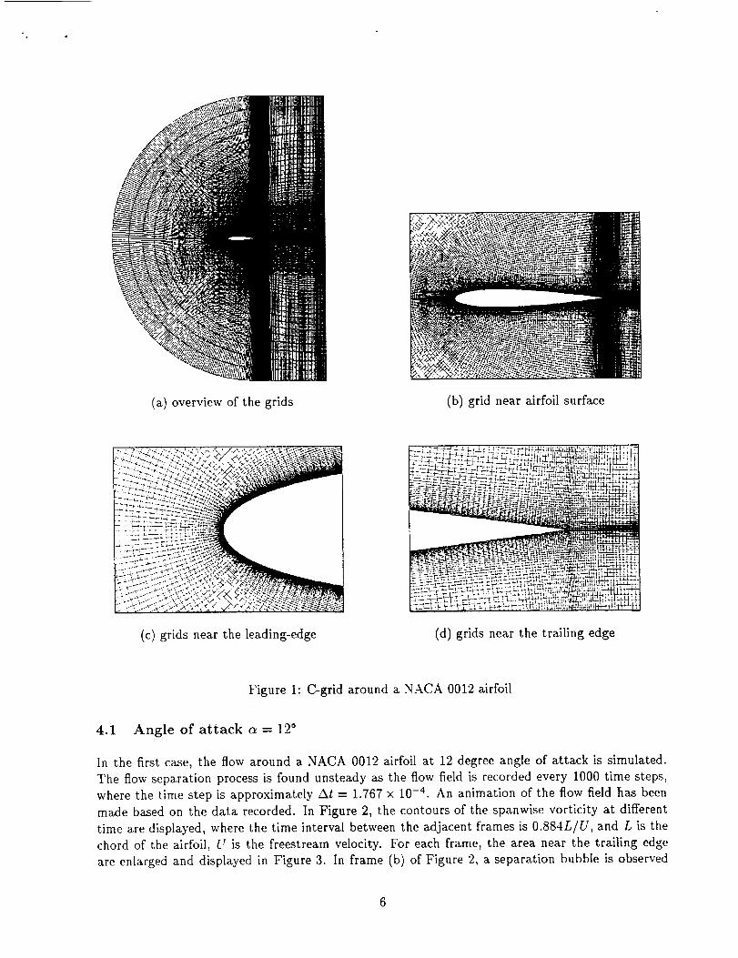
In Figure 1, the body-fitted C-grid around a NACA 0012 airfoil is displayed. The grids are

orthogonal at the boundaries. The distribution of the grids near the leading-edge and trailing-edge

are also depicted by Figure 1(c) and (d), where good orthogonality has been achieved.

4 Results and Discussions

The situation of an airfoil with a high angle of attack occurs in many applications which are of

particular interest. In these cases, the fluid flow around the airfoil becomes very unstable and

different eddy structures are formed in the vicinity of the airfoil. These eddy structures severely

affect the airfoil's aerodynamic properties. Vortex interactions, such as vortex pairing, and the

interactions between the airfoil and vortex, lead to noise generation. In our simulation, two angles

of attack have been chosen, the first one is c_ = 12°, the second one is c_ = 20 °. For both cases, the

Reynolds number is Re = 5 × 10s, based on the chord length L and freestream velocity U.

(a) overview of the grids (b) grid near airfoil surface

- " -"-_ ...... _"_-'_il:_

(c) grids near the leading-edge (d) grids near the trailing edge

Figure 1: C-grid around a NACA 0012 airfoil

4.1 Angle of attack a = 120

In the first case, the flow around a NACA 0012 airfoil at 12 degree angle of attack is simulated.

The flow separation process is found unsteady as the flow field is recorded every 1000 time steps,

where the time step is approximately At = 1.767 x 10 -4. An animation of the flow field has been

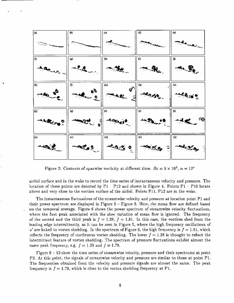
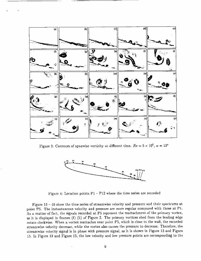
made based on the data recorded. In Figure 2, the contours of the spanwise vorticity at different

time are displayed, where the time interval between the adjacent frames is 0.884L/U, and L is the

chord of the airfoil, U is the freestream velocity. For each frame, the area near the trailing edge

are enlarged and displayed in Figure 3. In frame (b) of Figure 2, a separation bubble is observed

6

nearthe leadingedge.The leading-edge separation bubble is formed when the laminar boundary

layer separates from the surface as a result of the strong adverse pressure gradient downstream

of the point of minimum pressure. The separation bubble is unstable. Vortical structures shed

from the separation and move downstream along the airfoil surface. These vortical structures are

called the primary vortices. The primary vortices shed from the leading are rolling clockwise and

moving downstream at the same time. Strong shear layers with reversed vorticity are generated

near the wall below the primary vortices as a result of the induced motion of these vortices. For

example, in the vicinity of leading edge in frames (e) (i) (p) (q) of Figure 2, this phenomenon is

quite clear. The primary vortices are pushed away from the wall by the induced reversed vorticity.

Some primary vortices reattach on the airfoil surface where they encounter a slower convection

velocity and slow down in motion to downstream. These reattached primary vortices are caught by

upstream vortices which are moving faster downstream, and vortex merge happens when the vortex

undergoing reattachment is overtaken by an upstream vortex with the same rotating direction andthe two vortices eventually merge in one large vortex rotating in the original direction; (see frames

(e) (f) (h) (o) (p)). The reatta_hment of the primary vortex leads to strong interaction between

the vortex and the local boundary-layer and induces an upstream accumulation and eruption of a

reversed boundary-layer vorticity. The reversed vorticity interacts with the primary vortex to form

a counter-rotating vortex pair. The reversed vortex induces the primary vortex upward away from

the wall. The vortex pair move downstream more rapidly with a faster convection velocity. The

vortex pair can be seen in frames (g) (j) (n) (o) of Figure 2. The reattachment of the primary vortex

happens not only near the leading edge but also at the rear part of the suction surface. In frame (g)

of Figure 2, two vortex pairs are observed. The upstream one is formed by a primary reattachment

near the leading edge, while the downstream one is formed by a primary vortex reattachment at the

rear part of the airfoil. For each vortex pair, the interactions between these vortices lead to vortex

deformation shown in frame (h) of Figure 2, where the vortex system becomes very complex because

of the interaction and deformation. Similar phenomena of vortex pairing have been observed in

experiments, e.g. Shih, et al. (1992). Another interesting phenomenon is observed near the trailing

edge of the airfoil in frame (i) and (j) of Figure 2, where a strong counterclockwise rotating vortex

is generated by the sweeping of the clockwise rotating vortex system over the trailing edge. Whenthe clockwise rotating vortex shed from the leading edge reaches the trailing edge, it induces a

local low pressure which drives the lower surface separating layer across the wake and curve into

the upper surface. This lower surface shear layer quickly rolls into the intense counterclockwise

vortex. This process can be seen more clearly in frame (h) and (i) of Figure 3. This phenomenon

was also observed in experiments (Shih, et al. 1992, 1995). The experimental results and our DNS

results agree well qualitatively. The quantitative comparison is improper because of the difference in

Reynolds number. Strong shear layer appears near the downstream edge of this large-scale trailing

edge vortex. Because of the instability of the shear layer, a chain of small-scale vortical structuresappear along the edge of the large-scale vortex. The structure of these small-scale vortices are

similar to that of the Kelvin-Helmholtz type instability. The large-scale vortex moves away from

the trailing edge as a result of the self-induced motion, and eventually detaches from the trailing

edge, as it is displayed in frames (i) to (k) of Figure 3. A similar process of the generation and

detachment of the trailing edge vortex can also be found through frames (u) to (x) in Figure 3.

The continuous generation of the trailing edge vortex is quasi-periodic. The interactions between

the vortex system are very complex and severe deformations are observed in frames (h) (i) (p) (q)

(s) (t) (v) (x) of Figure 2. Near trailing edge, some of the typical vortex deformation are displayed

in frames (h) (i) (p) (q) of Figure 3.

To obtain the spectrum information about flow separation, twelve points are selected near the

l° llo i(v)

JIt tFigure2: Contours of spanwise vorticityat differenttime. Re --5 × 105,_ --12°

airfoil surface and in the wake to record the time series of instantaneous velocity and pressure. The

location of these points are denoted by Pl - P12 and shown in Figure 4. Points Pl - Pl0 locate

above and very close to the suction surface of the airfoil. Points Pll, P12 are in the wake.

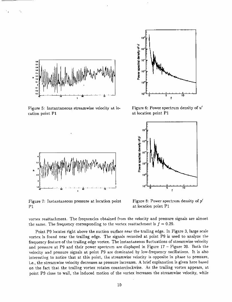
The instantaneous fluctuations of the streamwise velocity and pressure at location point P1 and

their power spectrum are displayed in Figure 5 - Figure 8. Here, the mean flow are defined based

on the temporal average. Figure 6 shows the power spectrum of streamwise velocity fluctuations,

where the first peak associated with the slow variation of mean flow is ignored. The frequency

of the second and the third peak is f = 1.28, f = 1.81. In this case, the vortices shed from the

leading edge intermittently, as it can be seen in Figure 5, where the high frequency oscillations of

u' are linked to vortex shedding. In the spectrum of Figure 6, the high frequency is f = 1.81, which

reflects the frequency of continuous vortex shedding. The lower f = 1.28 is thought to reflect the

intermittent feature of vortex shedding. The spectrum of pressure fluctuations exhibit almost the

same peak frequency, e.g. f = 1.28 and f = 1.79.

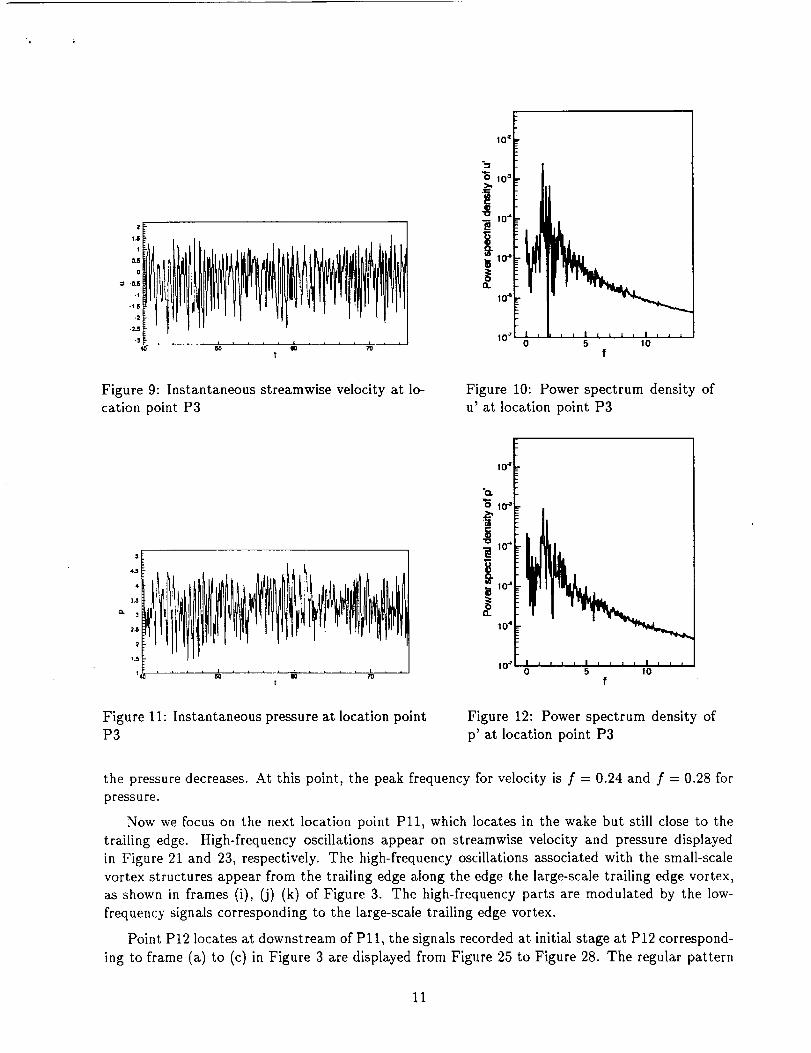
Figure 9 - 12 show the time series of streamwise velocity, pressure and their spectrumsat point

P3. At this point, the signals of streamwise velocity and pressure are similar to those at point Pl.

The frequencies obtained from the velocity and pressure signals are almost the same. The peak

frequency is f = 1.70, which is close to the vortex shedding frequency at Pl.

.. (p) <,olI (,)1/ (,)1 (,)1

Figure 3: Contours of spanwise vorticity at different time. Re = 5 x 10 5, a = 12 °

Pl P2 P]

PlO Pl] P12P7

Figure 4: Location points P1 - P12 where the time series are recorded

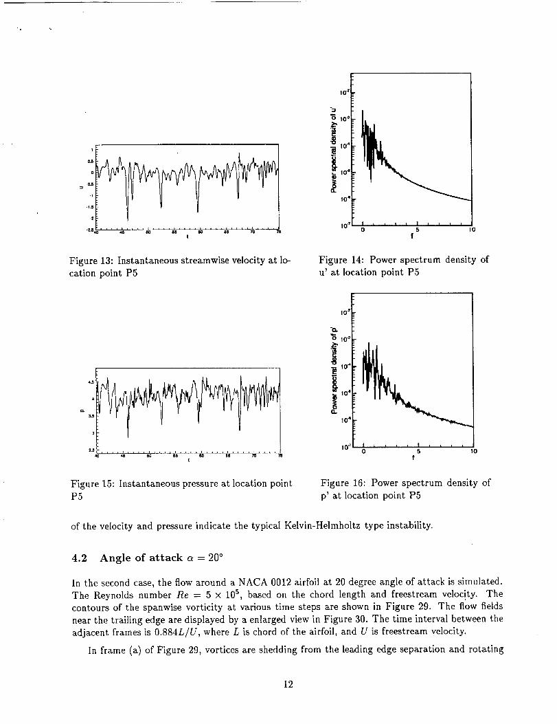
Figure 13 - 16 show the time series of streamwise velocity and pressure and their spectrums at

point P5. The instantaneous velocity and pressure are more regular compared with those at P1.

As a matter of fact, the signals recorded at P5 represent the reattachment of the primary vortex,

as it is displayed in frames (f) (h) of Figure 2. The primary vortices shed from the leading edge

rotate clockwise. When a vortex reattaches near point PS, which is close to the wall, the recorded

streamwise velocity decrease, while the vortex also causes the pressure to decrease. Therefore, the

streamwise velocity signal is in phase with pressure signal, as it is shown in Figure 13 and Figure

15. In Figure 13 and Figure 15, the low velocity and low pressure points are corresponding to the

r •

oJ

0.1

oJs

o.4

o.3

o-2

o.1

o

-o.1

-0.2

.0.3

t

Figure 5: Instantaneous streamwise velocity at lo-

cation point P1

I0"=

10 _

10"

O.

10 4

I0"InlmnlJnnvlJ_

0 5 I0

l

Figure 6: Power spectrum density of u'

at location point P1

3

2

4_

I0=

"a.

io _

"o_ 10 _

R_

,_ m"

O.

10 4

10 q I t I , , I , , , , I , ,

eo .... __ 0 5 10z f

Figure 7: Instantaneous pressure at location pointP1

Figure 8: Power spectrum density of p_

at location point P1

vortex reattachment. The frequencies obtained from the velocity and pressure signals are almost

the same. The frequency corresponding to the vortex reattachment is f = 0.29.

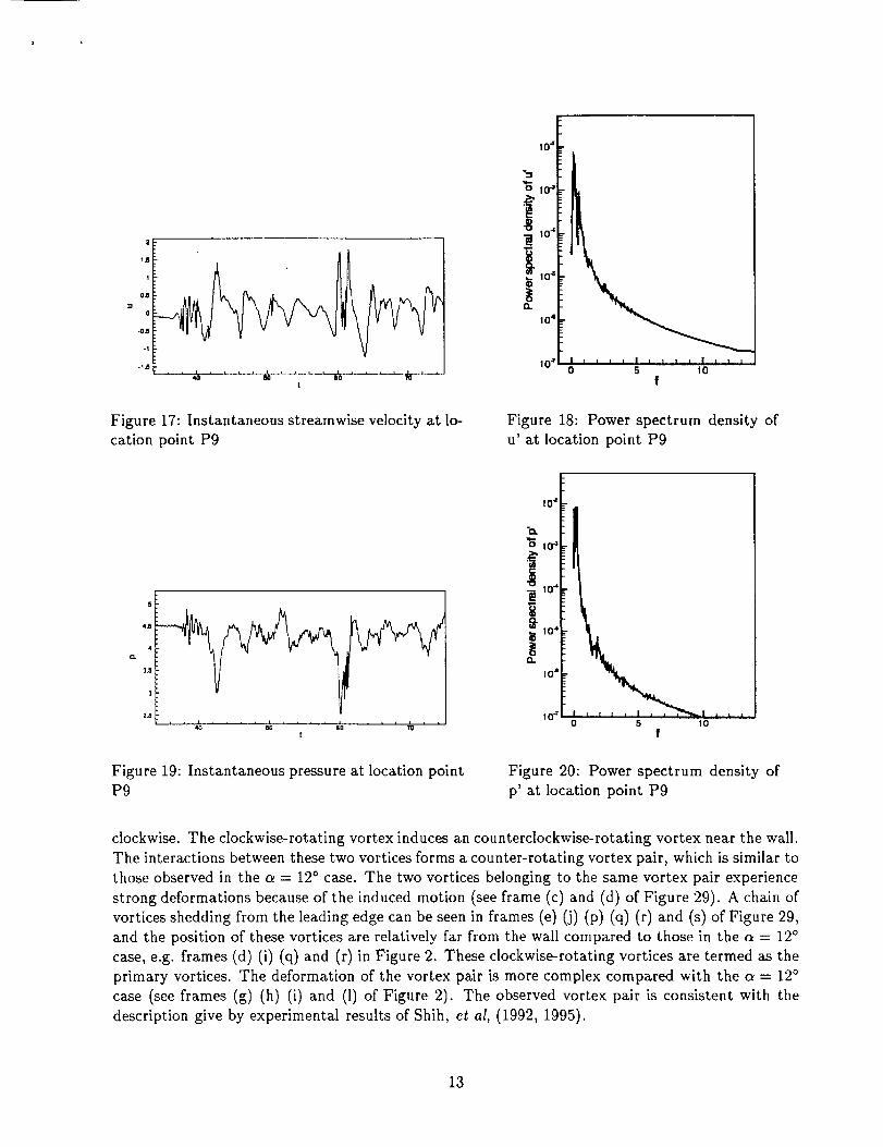
Point P9 locates right above the suction surface near the trailing edge. In Figure 3, large scale

vortex is found near the trailing edge. The signals recorded at point P9 is used to analyze the

frequency feature of the trailing edge vortex. The instantaneous fluctuations of streamwise velocity

and pressure at P9 and their power spectrum are displayed in Figure 17 - Figure 20. Both the

velocity and pressure signals at point P9 are dominated by low-frequency oscillations. It is also

interesting to notice that at this point, the streamwise velocity is opposite in phase to pressure,

i.e., the streamwise velocity decreases as pressure increases. A brief explanation is given here based

on the fact that the trailing vortex rotates counterclockwise. As the trailing vortex appears, at

point P9 close to wall, the induced motion of the vortex increases the streamwise velocity, while

10

2

10: OS

-15

2

2J

$ .... I 1 l , , I t40 50 an ___ 7V ___--.L--

t

!0_ I

iOz-- I k _ , I _ , _ , I , ,0 5 10

f


cation point P3

s

45

4

3

L i , i l J _--, • , ,_ -.,_ , ,[

Figure 10: Power spectrum density of

u' at location point P3

.0. 10_ I

"6 m-o

!,°.[lO

I 0 '_ ' '0

_]= ii=l ,,t

5 IOf



p' at location point P3

the pressure decreases. At this point, the peak frequency for velocity is f = 0.24 and f = 0.28 for

pressure.

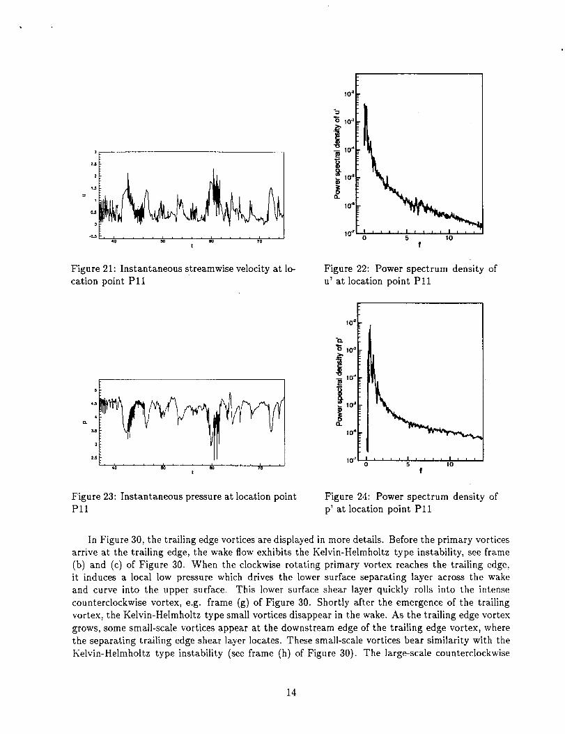
Now we focus on the next location point Pll, which locates in the wake but still close to the

trailing edge. High-frequency oscillations appear on streamwise velocity and pressure displayed

in Figure 21 and 23, respectively. The high-frequency oscillations associated with the small-scale

vortex structures appear from the trailing edge along the edge the large-scale trailing edge vortex,

as shown in frames (i), (j) (k) of Figure 3. The high-frequency parts are modulated by the low-

frequency signals corresponding to the large-scale trailing edge vortex.

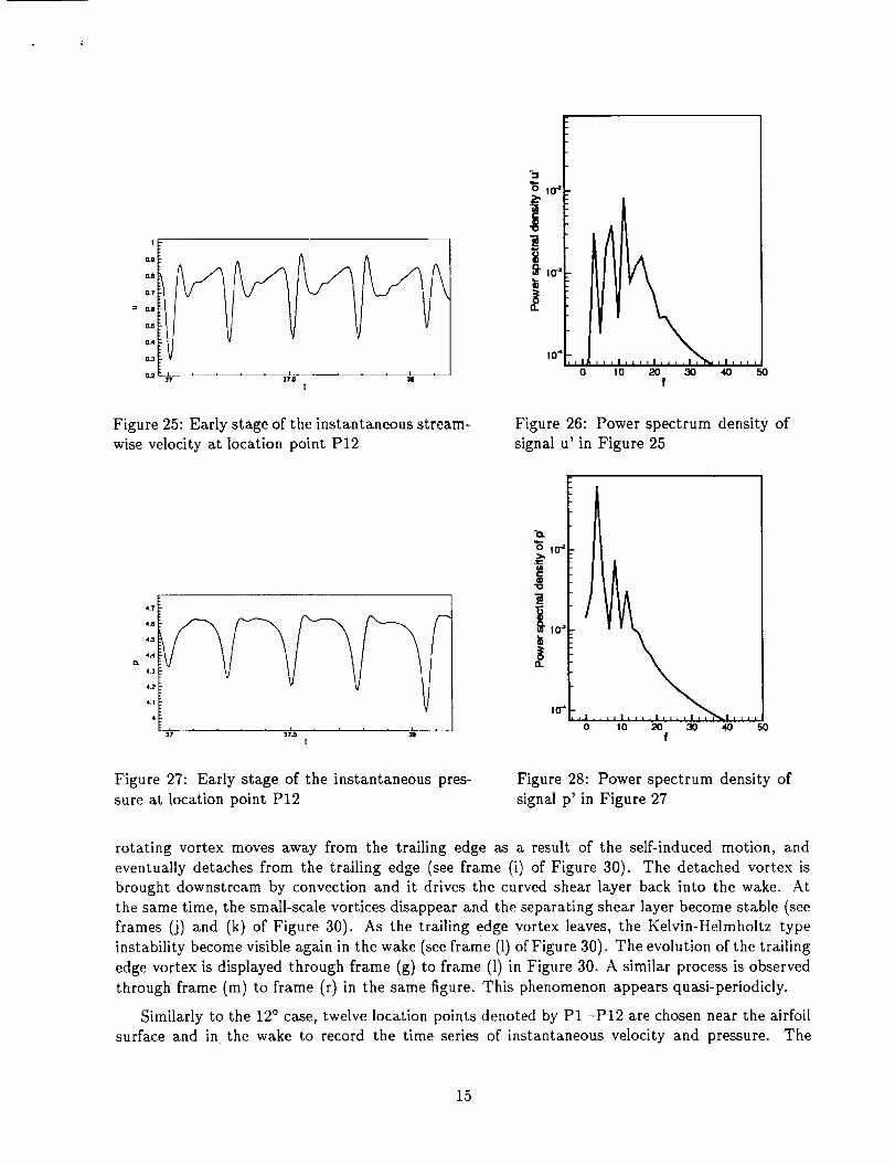
Point P12 locates at downstream of Pll, the signals recorded at initial stage at P12 correspond-

ing to frame (a) to (c) in Figure 3 are displayed from Figure 25 to Figure 28. The regular pattern

11

1

0

-0.5=

-1

-1..5

-2,_, , , _ .... _ ....• 5o _'_.... _," ' 'o'_.... __t


cation point P5

10_

10_104

10 4

|0: 1 z , = z ] z z z z I0 5 I0

f



4

0.3.5

3

t

Figure 15: Instantaneous pressure at location point

P5

10_

"0.

10-_

10"

to_

1o4

1o' I i ; i i I ,o 5

fIo



of the velocity and pressure indicate the typical Kelvin-Helmholtz type instability.

4.2 Angle of attack a = 20 °

In the second case, the flow around a NACA 0012 airfoil at 20 degree angle of attack is simulated.

The Reynolds number Re = 5 × 105, based on the chord length and freestream veloc!ty. The

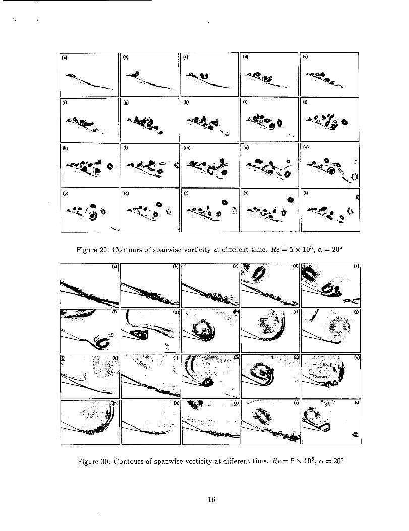
contours of the spanwise vorticity at various time steps are shown in Figure 29. The flow fields

near the trailing edge are displayed by a enlarged view in Figure 30. The time interval between the

adjacent frames is 0.884L/U, where L is chord of the airfoil, and U is freestream velocity.

In frame (a) of Figure 29, vortices are shedding from the leaxting edge separation and rotating

12

2

1

0.8

0

_n.5 !

-1.6

40 r.n IO[


cation point P9

10 _

"5 !0 -_

fflr-

10"*

n

104

10= l_,_,IIlllIlll

0 5 10f



5

4,5

4

3

t


10*

"5 10_

r-

"_ 10_E

10"_

o.

lO4

lO0 5 10

f

L L I



clockwise. The clockwise-rotating vortex induces an counterclockwise-rotating vortex near the wall.

The interactions between these two vortices forms a counter-rotating vortex pair, which is similar to

those observed in the _ = 12 ° case. The two vortices belonging to the same vortex pair experience

strong deformations because of the induced motion (see frame (c) and (d) of Figure 29). A chain of

vortices shedding from the leading edge can be seen in frames (e) (j) (p) (q) (r) and (s) of Figure 29,

and the position of these vortices are relatively far from the wall compared to those in the c_ -- 12°

case, e.g. frames (d) (i) (q) and (r) in Figure 2. These clockwise-rotating vortices are termed as the

primary vortices. The deformation of the vortex pair is more complex compared with the c_ = 12 °

case (see frames (g) (h) (i) and (l) of Figure 2). The observed vortex pair is consistent with the

description give by experimental results of Shih, et al, (1992, 1995).

13

]

2.5

2

1.5

1

0

t


cation point Pll

10_

10..o10_

! 0 4

i0 -_ i]|| fill ,,_

0 5 10f


u' at location point Pll

5

4

Q.

3.8

3

2.5

10_

'_ lo_

,I)

---_10"_

10_

a_

104

I 0 "7 l , , , , | I I l l J I I I0 5 I0

f

Figure 23: Instantaneous pressure at location pointPll


p' at location point Pll

In Figure 30, the trailing edge vortices are displayed in more details. Before the primary vortices

arrive at the trailing edge, the wake flow exhibits the Kelvin-Helmholtz type instability, see frame

(b) and (c) of Figure 30. When the clockwise rotating primary vortex reaches the trailing edge,

it induces a local low pressure which drives the lower surface separating layer across the wake

and curve into the upper surface. This lower surface shear layer quickly rolls into the intense

counterclockwise vortex, e.g. frame (g) of Figure 30. Shortly after the emergence of the trailing

vortex, the Kelvin-Helmholtz type small vortices disappear in the wake. As the trailing edge vortex

grows, some small-scale vortices appear at the downstream edge of the trailing edge vortex, where

the separating trailing edge shear layer locates. These small-scale vortices bear similarity with the

Kelvin-Helmholtz type instability (see frame (h) of Figure 30). The large-scale counterclockwise

14

0.g

= 0.6

0

0.4O.3

0.23"/ 37J5 31

[

Figure 25: Early stage of the instantaneous stream-

wise velocity at location point P12

-=

"6 lo'

10_

O.

10"

0 4O 5OII,

10 20 30f


signal u' in Figure 25

4.'/

4.e

4.5

4.4O.

4,3

4.2

4.1

4

1'7 ' _;_ _ -_---'_--[

"0 I

lO_ ,, , , I, ,, ,

0 10 20 30 40 50

f

Figure 27: Early stage of the instantaneous pres-

sure at location point P12


signal p' in Figure 27

rotating vortex moves away from the trailing edge as a result of the self-induced motion, and

eventually detaches from the trailing edge (see frame (i) of Figure 30). The detached vortex is

brought downstream by convection and it drives the curved shear layer back into the wake. At

the same time, the small-scale vortices disappear and the separating shear layer become stable (see

frames (j) and (k) of Figure 30). As the trailing edge vortex leaves, the Kelvin-Helmholtz type

instability become visible again in the wake (see frame (l) of Figure 30). The evolution of the trailing

edge vortex is displayed through frame (g) to frame (1) in Figure 30. A similar process is observed

through frame (m) to frame (r) in the same figure. This phenomenon appears quasi-periodicly.

Similarly to the 12 ° case, twelve location points denoted by P1 -P12 are chosen near the airfoil

surface and in the wake to record the time series of instantaneous velocity and pressure. The

15

(i)

" __,ll. °

_)

".411

C,:) (o')

(!,)

Ci,) CI) C_)

(i) (.1")

(_ (o)

Figure 29: Contours of spanwise vorticlty at different time. Re = 5 x l0 s, el = 20 °

(c)

I, _.- _::_. (t)

Figure 30: Contours of spanwise vorticity at different time. Re = 5 × l0 s, _ = 20 °

16

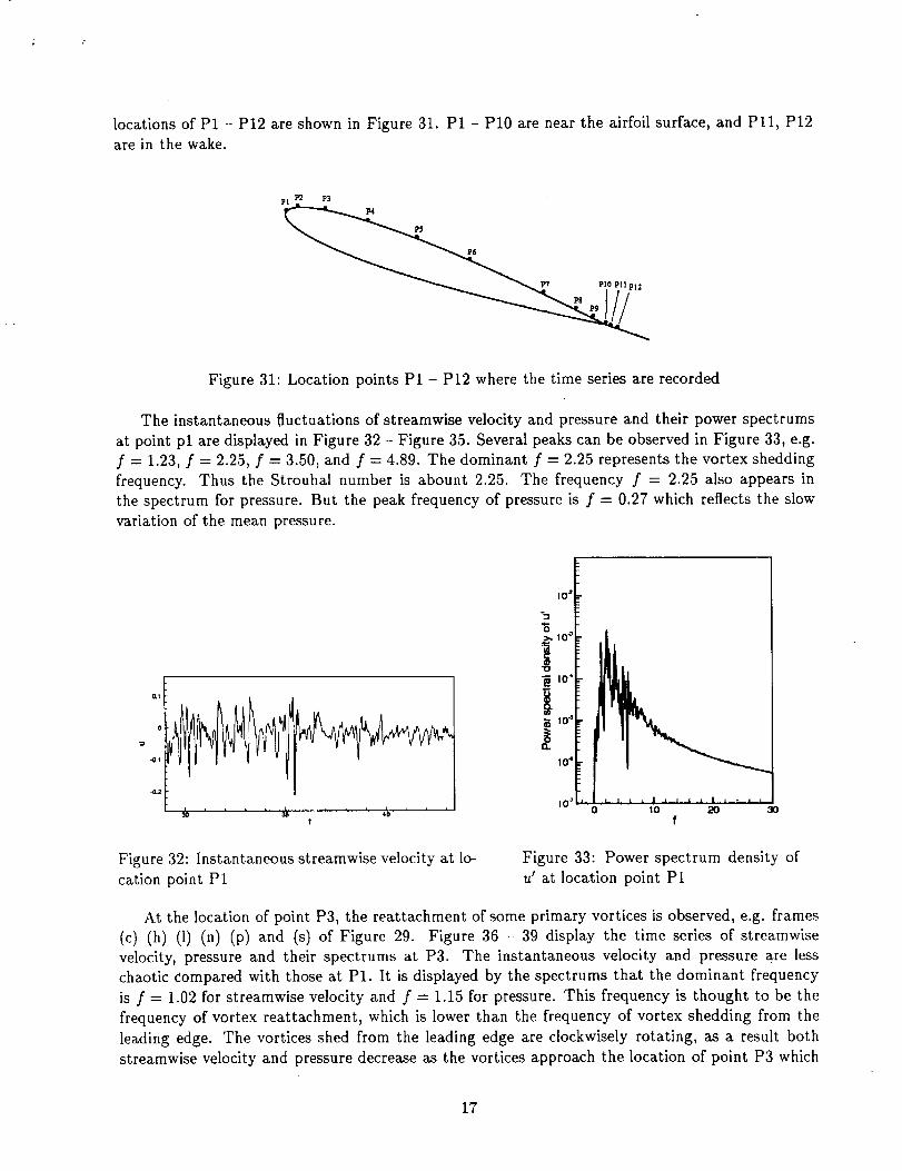
locations of P1 - P12 are shown in Figure 31. P1 - P10 are near the airfoil surface, and Pll, P12

are in the wake.

PI P2 P3 P4 P$ P6

_P7 PIO Pllpl 1

Figure 31: Location points P1 - P12 where the time series are recorded

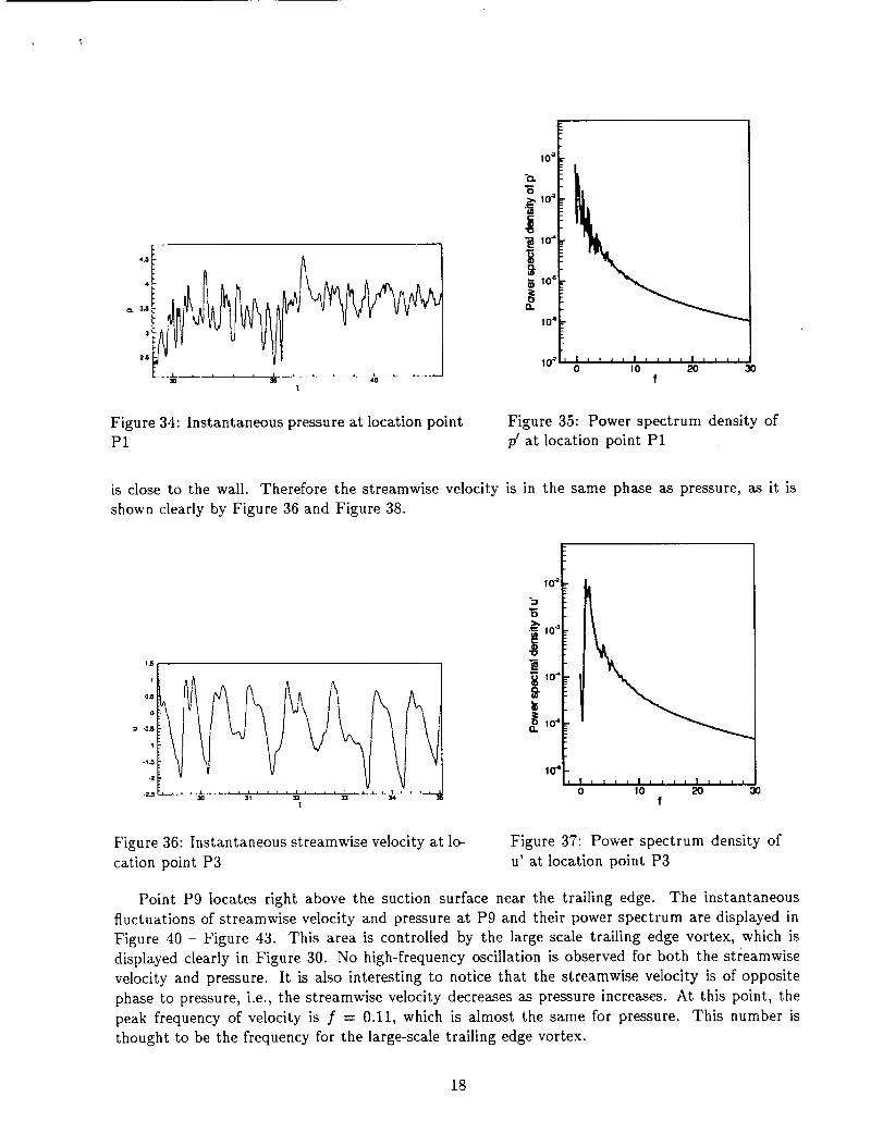
The instantaneous fluctuations of streamwise velocity and pressure and their power spectrums

at point pl are displayed in Figure 32 - Figure 35. Several peaks can be observed in Figure 33, e.g.

/ = 1.23, / = 2.25, / = 3.50, and / = 4.89. The dominant / = 2.25 represents the vortex shedding

frequency. Thus the Strouhal number is abount 2.25. The frequency / = 2.25 also appears in

the spectrum for pressure. But the peak frequency of pressure is f = 0.27 which reflects the slow

variation of the mean pressure.

o.t

o

-oJ

,j,l_

!

- i0_I

!i:ir1G" '

0 tO 20f


cation point P1



At the location of point P3, the reattachment of some primary vortices is observed, e.g. frames

(c) (h) (1) (n) (p) and (s) of Figure 29. Figure 36 - 39 display the time series of streamwise

velocity, pressure and their spectrums at P3. The instantaneous velocity and pressure are less

chaotic compared with those at P1. It is displayed by the spectrums that the dominant frequency

is / = 1.02 for streamwise velocity and f = 1.15 for pressure. This frequency is thought to be the

frequency of vortex reattachment, which is lower than the frequency of vortex shedding from the

leading edge. The vortices shed from the leading edge are clockwisely rotating, as a result both

streamwise velocity and pressure decrease as the vortices approach the location of point P3 which

17

4.5

4

Q. 325

3

t


10_

>, I0 _

"_ 10"

10"_

(3.

10"

10'

\

lltllllll[lllll

0 !0f


p_ at location point P1

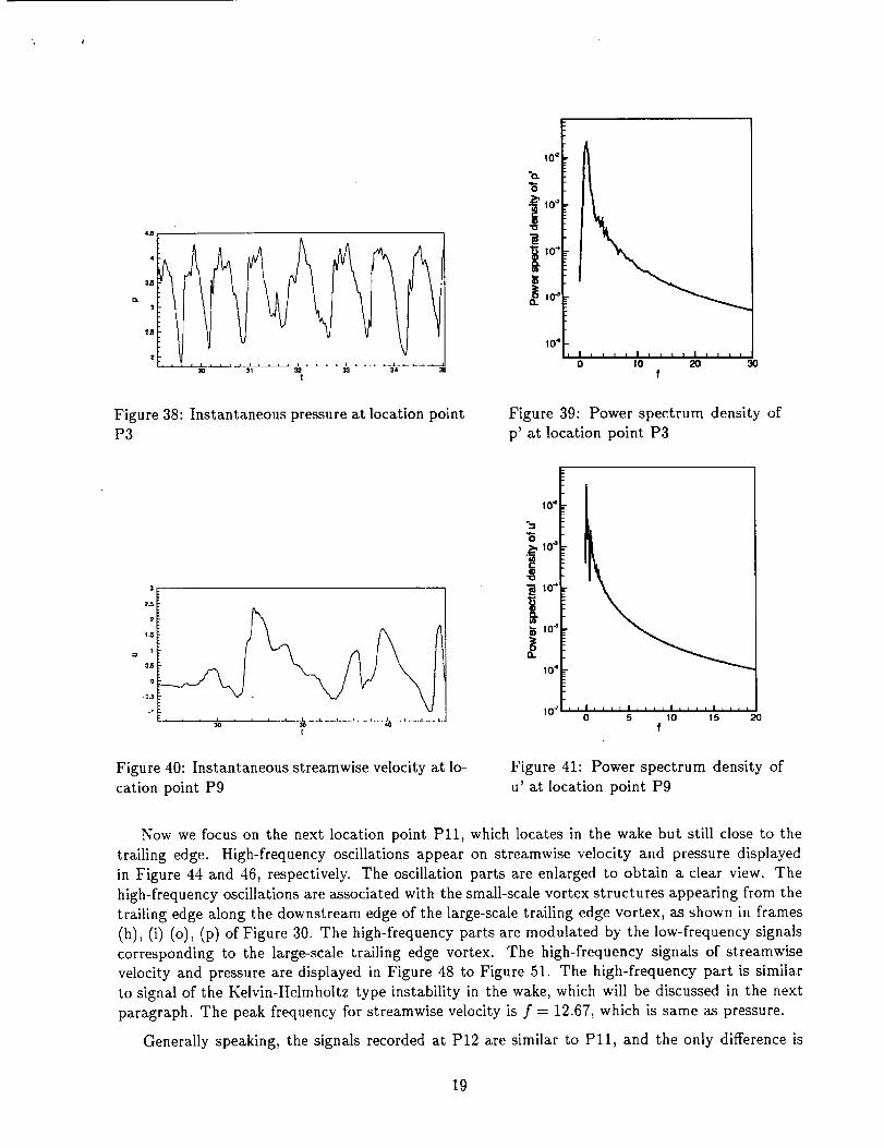
is close to the wall. Therefore the streamwise velocity is in the same phase as pressure, as it is

shown clearly by Figure 36 and Figure 38.

125

1

0,5

0

-O.5

-I

-2

-2._ 34 35t

I0 _

"6i0 _

tO_

104I , l , i I , i i l I i i i ,

0 I0 20f

30


cation point P3



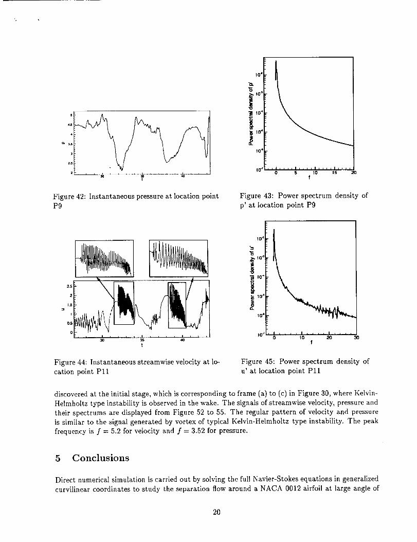
Point P9 locates right above the suction surface near the trailing edge. The instantaneous

fluctuations of streamwise velocity and pressure at P9 and their power spectrum are displayed in

Figure 40 - Figure 43. This area is controlled by the large scale trailing edge vortex, which is

displayed clearly in Figure 30. No high-frequency oscillation is observed for both the streamwise

velocity and pressure. It is also interesting to notice that the streamwise velocity is of opposite

phase to pressure, i.e., the streamwise velocity decreases as pressure increases. At this point, the

peak frequency of velocity is f = 0.11, which is almost the same for pressure. This number is

thought to be the frequency for the large-scale trailing edge vortex.

18

4

3

2,5

t


P3

tO_

"o.

"5

' 10-_

!Q. tO "_

104I,_,tl,_:]l,_:,

0 tOf

3O



3

2.5

3

1.t

U.5

0

-0.5

-1

r


cation point P9

10_

._,!0 "_

'_ 10"*

_G tO'a

(3-

104

10 _ ,_I,TY_Ib,,_I_,,I_,_0 5 10 15

f20



Now we focus on the next location point Pll, which locates in the wake but still close to the

trailing edge. High-frequency oscillations appear on streamwise velocity and pressure displayed

in Figure 44 and 46, respectively. The oscillation parts are enlarged to obtain a clear view. The

high-frequency oscillations are associated with the small-scale vortex structures appearing from the

trailing edge along the downstream edge of the large-scale trailing edge vortex, as shown in frames

(h), (i) (o), (p) of Figure 30. The high-frequency parts are modulated by the low-frequency signals

corresponding to the large-scale trailing edge vortex. The high-frequency signals of streamwise

velocity and pressure are displayed in Figure 48 to Figure 51. The high-frequency part is similar

to signal of the Kelvin-Helmholtz type instability in the wake, which will be discussed in the next

paragraph. The peak frequency for streamwise velocity is f = 12.67, which is same as pressure.

Generally speaking, the signals recorded at P12 are similar to Pll, and the only difference is

19

5

4.5

4

Q" 3.5

3

2J

2

t

104

"o.

._10 "_

"0

-_ 10 "L

104

10 4

i0 _ I1[ ''''1.*''1''''1''''0 5 10 15

f


P9



O."L T i | .... ! .... I , _

30 35 40

t

I0 _

.

"6._, 10":

I0"

10_

O.

10 4

10 "7I , , , _ I , l , , I _ l ] ,

0 i0 _0 30f


cation point Pll


u' at location point Pll

discovered at the initial stage, which is corresponding to frame (a) to (c) in Figure 30, where Kelvin-

Helmholtz type instability is observed in the wake. The signals of streamwise velocity, pressure and

their spectrums are displayed from Figure 52 to 55. The regular pattern of velocity and pressure

is similar to the signal generated by vortex of typical Kelvin-Helmholtz type instability. The peak

frequency is f = 5.2 for velocity and f = 3.52 for pressure.

5 Conclusions

Direct numerical simulation is carried out by solving the full Navier-Stokes equations in generalized

curvilinear coordinates to study the separation flow around a NACA 0012 airfoil at large angle of

2O

t

"_ lO.a_

10 4

10' Illllllllllllll

o tof

3o

Figure 46: o

nInstantaneous pressure at location point Pll


p' at location point Pll

1.;'5

Figure 48: High-frequency part of the instanta-

neous streamwise velocity at location point Pll

104

"_lff:

_ I0"

D... 10_

10450 I00

f



attack. By using a fourth-order centered compact scheme for spatial discretization, the small-scale

vortical structures are resolved, which will dissipate if low-order numerical schemes are used. Non-

reflecting boundary conditions are imposed at the far-field and outlet boundaries to avoid possible

non-physical wave reflection.

The DNS results clearly describe the flow separation process at the suction surface of the

airfoil. The phenomena of the leading edge separation, vortex shedding, vortex reattachment,

vortex pairing, generation of large-scale trailing edge vortex, and small-scale vortices associated with

the Kelvin-Helmholtz type instability are observed through the DNS database. These phenomena

are consistent with the experimental results obtained by Shih, et al, (1992, 1995). Based on the

spectral analysis, the vortex shedding frequency, the frequency of the first vortex reattachment, and

21

4

3_

3

2.5

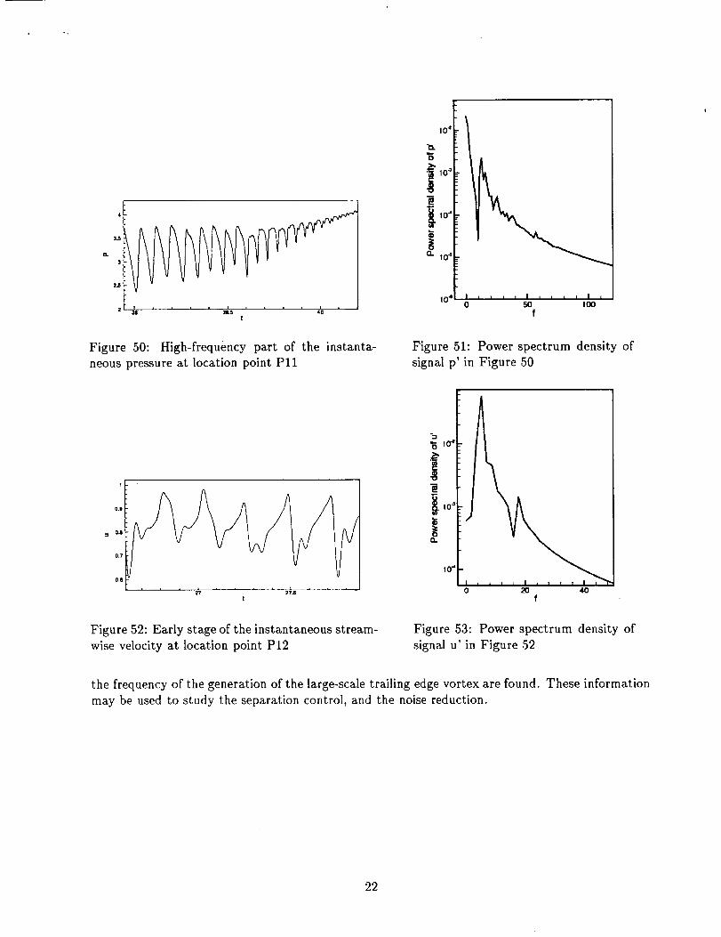
Figure 50: High-frequency part of the instanta-

neous pressure at location point Pll

"5

10-=

I0"

a. I04

10 4 I , , , , I , , , _ I ,0 50 100

f



'ii

0.8!

0.7

0.8

Figure 52: Early stage of the instantaneous stream-

wise velocity at location point P12

"6

I 0 "4 -

I

0z

20 40f



the frequency of the generation of the large-scale trailing edge vortex are found. These information

may be used to study the separation control, and the noise reduction.

22

4_7

_8

_. 4.4

4.3

4.2

4,1

427 2T5

!

o.

r-4)

"0

0

!o _

I

o'''Illli|ll

40f

Figure 54: Early stage of the instantaneous pres-

sure at location point P12Figure 55: Power spectrum density of


23

References

[1] Arena, A. V., and Muellet, T. J. 1980. laminar separation, transition, and turbulent reattach-

merit near the leading edge of airfoils. AIAA Journal, 18(7), pp.747-753

[2] Jiang, L., Shah, H, Liu, C., Visbal, M. R. 1999. Non-reflecting boundary condition in curvilin-

ear coordinates, Second AFOSR International Conference on DNS/LES, Rutgers, New Jersey,

June 7-9.

[3] LeLe, S. K. 1992. Compact finite difference schemes with spectral-like resolution. J. Comput.

Phys. 103, pp.16-42.

[4] Shih, C., Lourenco, L., Van Dommelen, L., and Krothapalli, A. (1992) Unsteady flow past an

airfoil pitching at a constant rate. AIAA Journal, 30(5), pp.1153-1161

[5] Shih, C., Lourenco, and Krothapalli, A. (1995) Investigation of flow at leading and trailing

edge of pitching-up airfoil. AIAA Journal, 30(5), pp.1369-1376

[6] Spekreijse, S.P. (1995) Elliptic grid generation based on Laplace equations and algebraic trans-

formation. J. Comp. Phys., 118, pp.38-61

[7] Tenaud, C., and Phuoc, L. T. 1997. Large eddy simulation of unsteady, compressible, separated

flow around NACA 0012 airfoil. Lecture Notes in Physics. 490, pp.424-429.

[8] Thompson, J. F., Warsi, Z. U. A., and Mastin, C. W. 1985. Numerical Grid Generation:

Foundations and Applications. Elsevier, New York

[9] Wu, J-Z., Lu, X., Denny, A. G., Fan, M., and Wu, J-M. 1999. Post-stall flow control on an

airfoil by local unsteady forcing. J. Fluid Mech., 371, pp.21-58.

[10] Yoon, S., Kwak D. 1992. Implicit Navier-Stokes solver for three-dimensional compressible flows,

AIAA Journal 30, pp.2653-2659

24

report - ntrs.nasa.gov

Documents