report of the long term national acid deposition

1

Report of the Long Term National Acid Deposition Monitoring

in Japan (JFY2003-2007)

MARCH 2009

Ministry of the Environment

Government of Japan

2

Ogasawara acid deposition monitoring site Samplers (Tokyo site)

Soil sampling (Hakusan, Ishikawa) In-land water sampling (Nagatomi-ike, Kagawa)

Sampling of river water flow in Ijira Lake Throughfall sampling at Ijira (Koubora gawa)

3

Yellow sand from continent Volcanic fumes from Asama Mt.

(18 Apr. 2006) (16 Sep. 2004) Pictures by MODIS mounted in Terra and Aqua earth observation satellite of NASA

(Provided from Japan Aerospace Exploration Agency)

Distribution of NO2 concentration in the troposphere in East

Asia by GOME

The upper figure shows the average concentration in January

1996 and the lower in January 2002. The grey parts show no

data.（Japan Agency for Marine-Earth and Technology, 2005）

Nitrogen annual deposition quantity

distribution (2002)

(Uno, et al., 2007)

4

The simulation results of the transboundary pollution of ozone in East Asia

(7 – 9 May 2007)

(Ohara, et al., 2008)

The distribution of seasonal global ozone by satellite observation

(Fishman.J, et al., 1997)

6

INTRODUCTION About acid deposition, acidification of lakes and forest damage became a diplomatic issue in Europe in the 1960s, and wet acidic air pollution became a problem in Japan in the 1970s. Therefore, the Ministry of the Environment (former Environment Agency) began the acid deposition survey from Japanese Fiscal Year (JFY) 1983 to comprehend the condition and influence of acid deposition in Japan with the aim of preventing harmful influence from acid deposition. Also, in order to maintain the acid deposition monitorihng in wide-area for long term, “The long term monitoring plan of acid deposition” was formulated on March 2002. Based on the plan, the Ministry of the Environment has implemented wet/dry deposition monitoring, land water monitoring for lakes, and soil/vegetation monitoring cooperating with local governments since JFY 2003. This report shows the results of long term monitoring conducted from JFY 2003 to JFY 2007, in addition, summarizes the results of the intensive survey on Ijira lake catchment area of which the soil is known to be acidified, from JFY 2005 to JFY 2007 focused. In recent years, transboundary air pollution in North-East Asia is pointed out as one of the causes of widening area that photochemical oxidant warnings are announced and increasing its concentration. For these reasons, not only acid deposition but also transboundary air pollution including ozone and aerosol is growing concern. We reviewed the existing study results such as calculation results of atmospheric simulation models as well as the condition of transboundary air pollution. This report is summarized about the result of study conducted at the acid deposition committee and its atmospheric issues sub-group and ecological impact sub-group established in the Ministry of Environment. The related data was collected and analyzed at Acid deposition and oxidant research center and it organized four working groups (acid deposition analysis, ecological impact analysis, Ijira lake intensive survey, transboundary air pollution) to analyze and review the research results. We extend a special thank to everyone concerned who cooperated with conducting and summarizing this monitoring survey. March 2009 Global Environment Bureau Ministry of the Environment

7

Committee Members

Committee on Acid Deposition

AKIMOTO, Hajime (Chair)

Frontier Research System for Global Change Japan Agency for Marine-Earth Science and

Technology

DOKIYA, Yukiko Edogawa University

GOTO, Ryozo2 Japan Environmental Technology Association

HAKAMATA, Tomoyuki Hamamatsu Photonics K.K.

HARA, Hiroshi Tokyo University of Agriculture and Technology

HISATAKE, Masayoshi1 Japan Environmental Laboratories Association

(Kochi Prefectural Environmental Research Center)

HORII, Kazuo1 Niigata Prefectural Government

KATO, Hisakazu Nagoya University

MURANO, Kentaro

Hosei University

ODA, Takashi2 Japan Environmental Laboratories Association

(Kochi Prefectural Environmental Research Center)

OGURA, Norio Tokyo University of Agriculture and Technology

OHTA, Seiichi2 Kyoto University

SATAKE, Kenichi Rissho University

TOTSUKA, Tsumugu Japan Environmental Sanitation Center

TOYAZAKI, Yasuo1 Japan Environmental Technology Association

UEDA, Hiromasa Acid Deposition and Oxidant Research Center

YAMAMOTO, Shinichi1 Niigata Prefectural Government

1: only in JFY2007 2: only in JFY2008

8

Sub-committee on Atmosphere

AOKI, Masatoshi1 Tokyo University of Agriculture and Technology

DOKIYA, Yukiko Edogawa University

FUJITA, Shin-ichi Central Research Institute of Electric Power

Industry

HARA, Hiroshi (Chair) Tokyo University of Agriculture and Technology

HATAKEYAMA, Shiro Tokyo University of Agriculture and Technology

MATSUDA, Kazuhide Meisei University

MURANO, Kentaro Hosei University

GOTO, Ryozo1 Japan Environmental Technology Association

LI, Hu2 Japan Environmental Technology Association

OHIZUMI, Tsuyoshi Niigata Prefectural Institute of Public Health

and Environmental Sciences

SHIMIZU, Hideyuki National Institute for Environmental Studies

TANAKA, Shigeru Keio University

UEMATSU, Mitsuo Ocean Research Institute,University of Tokyo

UNO, Itsushi Kyushu University

1: only in JFY2007 2: only in JFY2008

Sub-committee on Ecological Impact

AKAMA, Akio

Forestry and Forest Products Research Institute

EBISE, Senichi Setsunan University

FUKUHARA, Haruo Niigata University


HATAKEYAMA, Shiro National Institute for Environmental Studies

IKEDA, Shigeto Forestry and Forest Products Research Institute

INOUE, Takanobu Gifu University

IZUTA, Takeshi Tokyo University of Agriculture and Technology

NAKAJIMA, Takuo Lake Biwa Research Institute

OGURA, Norio (Chair) Tokyo University of Agriculture and Technology

OHTA, Seiichi Kyoto University

SHIMIZU, Hideyuki National Institute for Environmental Studies

SHINDO, Junko National Institute of Agro-Environmental

Science

SUDA, Ryuichi Fukuoka Institute of Health and

Environmental Science

TAKAMATSU, Takejiro National Institute for Environmental Studies

TOTSUKA, Tsumugu Japan Environmental Sanitation Center

9

Working Group on Transboundary Air Pollution

AKIMOTO, Hajime (Chair)

Frontier Research System for Global Change Japan Agency for Marine-Earth Science and

Technology

UNO, Itsushi Kyushu University

OHARA, Toshimasa National Institute for Environmental Studies

HATAKEYAMA, Shiro National Institute for Environmental Studies

HARA, Hiroshi Tokyo University of Agriculture and Technology

YAMADI, Kazuyo Frontier Research System for Global Change Japan Agency for Marine-Earth Science and

Technology Working Group on Acid Deposition Analysis

HARA, Hiroshi(Chair) Tokyo University of Agriculture and Technology

AIKAWA, Masahide Hyogo Prefectural Institute of Public Health

and Environmental Science

OHIZUMI, Tsuyoshi

Niigata Prefectural Institute of Public Health and Environmental Sciences

TAKAMI, Akinori National Institute for Environmental Studies

TOMOYOSE, Yoshitaka Okinawa Prefectural Institute of Health and

Environment

NOGUCHI, Izumi Hokkaido Institute of Environmental Sciences

HAYASHI, Kentaro National Institute of Agro-Environmental

Science


Working Group on Ecological Impact Analysis

OGURA, Norio (Chair) Tokyo University of Agriculture and Technology

IKEDA, Shigeto Forestry and Forest Products Research Institute

SHINDO, Junko National Institute of Agro-Environmental

Science

TAKAMATSU, Takejiro National Institute for Environmental Studies


FUKUHARA, Haruo Niigata University

YAMADA, Toshiro National Institute of Public health

Working Group on Ijira-ko Intensive Survey

HAKAMATA, Tomoyuki(Chair) Hamamatsu Photonics K.K.

INOUE, Takanobu Gifu University

SUMIDA, Hiroshi Gifu Prefectural Research Institute for Health and

Environmental Sciences

TAKAHASHI, Masamichi Forestry and Forest Products Research Institute

NAKAHARA, Osamu Hokkaido University


CONTENTS

General overview of results of the survey 1．History of acid deposition survey

2．The purpose and contents of the research

3．Monitoring 3.1 Acid Deposition Monitoring

3.1.1 Wet Deposition Monitoring

3.1.2 Dry Deposition Monitoring

3.1.3 Synthetic consideration to acid deposition

3.2 Results of Ecological Impact Monitoring

3.2.1 Results of Soil and Vegetation Monitoring

3.2.2. Results of Monitoring on Inland Aquatic Environment

3.2.3 Discussion on ecological effects of acid deposition

3.3 Results of Ijira Intensive Surveys 3.4 Comparison with foreign monitoring data

4. Long-Range Trans-boundary Air Pollution

4.1 Status of transboundary air pollution in the world and East Asia 4.2 The Increasing Emissions of Air Pollutants in East Asia 4.3 Effect on trans-boundary air pollution in Japan

4.3.1 State of trans-boundary air pollution in Japan

4.3.2 Future prediction of impact of transboundary air pollution on Japan

4.4 Intercontinental transport of air pollutants and hemispheric air pollution 4.4.1 Task Force on Hemispheric Transport of Air Pollutants (CLRTAP/TF-HTAP)

4.4.2 Analysis by intercontinental transportation model

5．Future challenges of the counter measures to acid deposition

3

General overview of results of the survey

１．Overview of the survey

・The Ministry of the Environment has conducted the acid deposition survey in order to figure out the condition and influence of acid deposition in Japan since JFY 1983. Based on the long term monitoring plan of acid deposition which was formulated in March 2002, wet/dry deposition monitoring (31 sites), land water monitoring for lakes (11 sites), and soil/vegetation monitoring (25 sites) have been implemented since JFY 2003.

・ This report shows the results of long term monitoring of acid deposition conducted from JFY 2003 to JFY 2007 and summarizes the results of the intensive survey on Ijira lake catchment area of which the soil is known to be acidified, from 2005 to 2007. It also reviews the influence of the transboundary air pollution to Japan.

２．The state of acid deposition and transboundary air pollution

（１）The result of acid deposition monitoring

・ The averages of precipitation pH for 5 years at monitoring sits were in the range from pH 4.51 ( Ijira lake) to pH 4.96 (Ogasawara). The total average was pH 4.68. Acid deposition is still being monitored. Less than pH3.0, which is thought to give acute damage to plant, was not observed, but it is figured out that strong acidic precipitation less than pH4.0 made up 4.5% in total precipitation at 14 sites which have been conducted daily sampling.

・ Precipitation pH showed small changes yearly and relatively low in some monitoring sites in recent years, but it has tendency to remain at the same level in total at the sites which have been observed at for more than 10 years. After 2005, the concentration of nitrate ion in precipitation showed the tendency to increase.

・ The yearly amounts of the total acid deposition at 12 monitoring sites in Japan

were calculated. Non-sea-salt sulfur was in the range of 16～54mmol m-2 y-1 and nitrogen was in the range of 22～130mmol m-2 y-1.

・ The amount of acid deposition by precipitation increased in the side of the Sea of Japan of Honshu from late autumn to spring. Also, the concentration of sulfur dioxide in the atmosphere tended to increase markedly in Sea of Japan side and

4

western area of Japan. In these areas, it would appear that sulfur oxides and nitrogen oxides supplied into the atmosphere increased from late autumn to spring. The pollutants input from tne continent was suggested.

・ In Japan, the amount of non-sea-salt sulfate ion and nitrate ion deposited by precipitation was twice or three times larger than those in Europe and the United States. Also, the amount of hydrogen ion deposition was several times higher in Europe and the United States, and the highest among East Asia. It is because Japan has large precipitation and the rate of acid counteracted by basic material in the atmosphere and precipitation is low.

・ The quantity of non-sea-salt calcium ion deposition, concentration of PM10 in the atmosphere and calcium ion in aerosol hit the highest in spring all of the country, which suggests the influence of yellow sand.

・ The concentration of ozone increases in spring countrywide, which suggests the influence of transboundary air pollution. Also, the change of average value of ozone concentration across the ages tends to increase in the country.

（２）Review of research on transboundary air pollution ・ The recent atmospheric simulation models estimated that the rate of the

contribution of the transboundary air pollution to the amount of acid deposition in Japan is about 30 – 65% for non- sea-salt sulfur ion and about 35 – 60% for nitrate ion.

・ The influence of transboundary air pollution to the concentration of ozone in Japan fluctuates widely depending on land areas, seasons and dates. However, it appears that about 10 -20 % of the monthly average of ozone concentration on Japan’s main island in Spring season originates East Asia and estimated that about several ppb influence comes from Europe and the United States in springtime.

・ Also, it is predicted that yearly average of ozone concentration in Japan on 2020 will increase 2 – 6ppb compared to 2000 if the emission of air pollutant in China generally continue to increase under the business as usual scenario.

5

３．Impact to ecosystem

（１）The result of soil/vegetation monitoring ・ In 2007, there was the indication that some of the woods declines at 17 out of 25

monitoring sites, but it was not observed that acid deposition or acidified soil mainly caused the declination.

・There is a trend that the pH (H2O) on the surface and the second layer of the soil in Ijira lake had decreased from 1990 to 2004. The pH in the surface layer was an average of pH 3.9 which indicates that the level of aluminum ion which has impact to growth of plant dissolved out to the soil so that it is necessary to continue to monitor.

・ Soil acidification trend was not observed at other observation points in general although some change with the age was observed in a part of monitoring items.

（２）The result of land water monitoring ・ The acidity of the surface layer water of the lakes was in the range from pH 5.36

-7.34, and the alkalinity was from 0.017 – 0.512 meq/L. Futago, Meike (Nagano prefecture), Yasya (Fukui prefecture) and Sawano (Kyoto prefecture) lakes were under pH 5.8 and the alkalinity was under 0.030meq/L.. It can be said that they have high sensibility to acid but it was not seen clearly the influence of air deposition at all lakes.

・ The acidity at Kamagaya river which flows into Ijira lake had tendency to decrease from 1996 to 2003, but it remains around pH 7 after 2004. The concentration of nitrate ion on the surface layer water at Ijira and its inflow two rivers showed a significant increase.

４．The result of the intensive study at Ijira lake water area

・ The acid deposition monitoring survey from JFY 1988 to JFY 2002 found that the physicochemical change such as the decrease of pH value which would present the impact of acid deposition at the rivers input to the Ijira lake and the surrounding soil in Ijira lake catchment area. In order to make clear about the sign of acidify and its process, MOEJ conducted the survey of the inlet and outlet flow in the catchment area and the intensive monitoring at swollen rivers from JFY 2005 to JFY 2007..

6

・ From the following findings i – iii, acidify of the catchment area of Ijira lake was considered to stay continuing to be acidified by the reason that sulfur and nitrogen piled in the soil by acid deposition from the atmosphere flowed out to the rivers.

ⅰ The total quantity of nitrogen deposition in Ijira lake catchment area was estimated 18.2 – 28.7 kg-N ha-1 y-1 which exceeded the reference index of nitrate ion outlet to rivers in Europe, 10 kg-N ha-1 y-1. The high concentration of the flow out of the nitrate ion has continued after middle of 1990s. It was considered that this nitrate ion flow out with the large amount of nitrogen deposition contributed to the acidification of the rivers.

ⅱ By estimating the material balance at the catchment area, the outlets of sulfur was twice more than the inlets. It was considered that sulfur stored in the soil for years flowed out and contributed the acidification of the rivers.

ⅲ By the trend that concentration of sulfate and nitrate ion at the swollen rivers increased, it was indicated that sulfur and nitrate stored on the surface soil around the catchment area flowed out.

・ It is difficult to show the progress of future acidification quantitatively because the mechanism of the acidification around Ijira lake catchment area is complicated and it remains a matter to be solved scientifically.

・ Although it is considered that the status of acidification may affect to human health and ecosystem immediately, it is needed to conduct survey at any hot spot which would have high risk of acidification since there is concern that other water area same as Ijira lake suffers acidification.

５．Future tasks about prevention of acid deposition （１）Long term monitoring ・ The influence of acid deposition is comprehended by only long term monitoring,

and it is possible to appear the influence abruptly by storing over a certain amount of acid material load when lakes and soils have low buffer abilities.

（２）Promotion of international cooperation ・ Aiming to extend the action scope of EANET from the conventional acid

deposition monitoring to the management of the atmosphere environment in East Asia, it is necessary to establish the international cooperative relationship and

7

promote regional collaboration to prevent air pollution.

（３）Approach to the transboundary air pollution ・ The transboundary air pollution from East Asia Continent is pointed out as one of

the reason of widening area that photochemical oxidant caution was announced in, rising ozone concentration gradually of and increasing in frequency of the detection of yellow sand. It is needed that the transboundary air pollution monitoring including not only acid deposition but also ozone and aerosol should be conducted.

（４）Promote the investigative study ・ In order to comprehend the influence and conditions of long range transboundary

air pollutions, it is necessary to promote research studies such as elaborating atmosphere simulation models, making high accuracy in emission inventory, deliberating reference index of sensibility of soil, vegetation and in-land-water and finding out hot spots with high risk in acidification.

8

１．History of acid deposition survey

Acid deposition is recognized as one of global environmental issues since the

substances causing acid deposition are transported over long distance and there is possibility that its influence diffuse to not only inside of the country but also to outside of the country. In Japan, our social concern to acid rain was risen because the fog and drizzle stimulated human eyes or skins and the rain had influence to crops like tobacco culture during rainy season in northern part of Kanto district from 1974 to 1976..

In Europe, it came to the surface that acid deposition acidified lakes in Northern Europe. The treaty for long distance transboundary air pollution was concluded in 1979. Joint monitoring of acid deposition and reducing emission of contaminated materials conducted based on the treaty have been successful.

Meanwhile, the emission of air contaminant has increased with rapid economic growth in East Asia. It is concerned that the transboundary air pollution including acid deposition will become more serious in the future. In order to promote the prevention method for acid deposition based on international cooperation in East Asia, EANET started functioning on a trial basis by Japanese initiative from April 1998 and has been running since January 2001. 13 countries in East Asia are joined now.

○ The domestic research about acid deposition

The Ministry of the environment established the acid deposition prevention committee whose members were consisted of the experts for air pollution, soil/vegetation, and land water, and has continued to conduct the research on acid deposition since 1983 in order to make clear the actual condition and the influence in our country.

As the result, “The general report about acid deposition research” was summed up on June 2004 as the research results conducted for twenty years from 1983 to 2002. It shows the following results.

① The acid depositions as high as those in Europe and the United States are

observed nationwide which is pH4.77 on an average. Also it was suggested that the contaminated materials flew into the area on the Sea of Japan side from the

9

continent. ② At this moment, it is not observed that acid depositions damage the ecosystem

such as vegetation erosion or acidify the soil. ③ The physicochemical changes of pH seemed to be caused by low level acid

deposition at Ijira lake water area, the rivers input to the lake and the surrounding lands where the ecosystem is thought to be fragile against acid depositions. However, these changes do not give any influence immediately to human health and the ecosystem of plants and water plants around the rivers,

As seen above, it is still unclear how acid depositions have an impact to the ecosystem in our country. However, the influence of acid deposition could become obvious in the future if we continue to have acid depositions as it is, because the influence of acid depositions to soil/vegetation and land water is considered to appear after long term period. Therefore, the Ministry of the Environment formulated “The long term monitoring plan of acid deposition” on March 2002 in order to maintain to monitor acid deposition in wide-area for long term, and has conducted the wet/dry deposition monitoring, the land water monitoring for lakes and soil/vegetation monitoring based on this plan.

Table1-1 Number of monitoring site

Phase 1 Phase 2 Phase 3 Phase 4 － long term

monitoring

Japanese

Fiscal

year

1983-1987

1988-1992 1993-1997 1998-2000 2001-2002 2003-2007

Wet/dry

deposition 14～34 29 48 55 48 31

Soil,

vegetation 12 43 88 20 18 25

in land

water

133

(screening) ５ 33 17 12 11

other 2(snow)

10

The relation between acid depositions and observed materials

Air contaminants such as sulfur dioxide or nitrogen oxide are oxidize to sulfur or nitric acids in the air, and come back to the land again (deposition). There are two types in the way of deposition. One is dissolved in rains or snow to be deposited (wet deposition). The other is deposited as the form of gas or particles called aerosol (dry deposition). Acid deposition as one of the environmental problems represents both wet deposition and dry deposition. Scientifically, it is called “acid deposition”.

As the damages by acid depositions, woods are diminishing by acidified soil, land water ecosystems have taken damages by acidified lakes and cultural properties like bronze statues and buildings become damaged. How much they have damage depends on the quantity of acid deposition. So in case of raining, we need to consider not only pH which shows the acid level but also amount of precipitation.

Ozone is known as air contaminant to exert a harmful influence to human health and plant. It is also an acidifying material which acidifies sulfur dioxide and nitrogen oxide very well. Therefore, the generation mechanism of acid depositions has close links to those of ozone.

Also, there are alkaline materials such as ammonia gas in the atmosphere. They generate sulfur ammonia and nitrate ammonia when they react with sulfur and nitric acid. These materials become dry deposition as aerosol or wet deposition dissolved in rains.

As seen above, it is important that “acid depositions” is regarded as the comprehensive air pollution which involves various materials. It is necessary to observe not only precipitation but also gas and related aerosol such as sulfur dioxide, nitrogen oxide, ozone, ammonia and soon.

11

２．The purpose and contents of the research

○ The purpose

The aim of the long term survey of acid depositions is to comprehend the influence of acid deposition early, the long distance transboundary of materials causing acid depositions and the long term trend. Also, it aims to find out the temporal and special changes and its influence in the quantity of acid deposition by monitoring acid deposition and its influence to ecosystem for long time periods with cooperating with EANET in order to predict the influence of acid depositions in the future. ○ The contents of the research

The Ministry of the Environment had conducted wet and dry acid deposition monitoring based on the plan of long term acid deposition survey in order to comprehend the condition of acid deposition, and soil/vegetation monitoring and land water monitoring in order to comprehend the influence of acid depositions to ecosystem from 2003 to 2007.

（１） Wet deposition monitoring Wet deposition monitoring was conducted at 31 points which were selected to be conducted acid deposition monitoring effectively and efficiently under consideration of the climate, aerial characteristics and the balance. The observation points are classified into 3 areas, which are remote, pastoral, and urban areas in accordance with the EANET wet deposition monitoring manuals (refer to figure 2-1). The precipitation samples (including snow) were collected with precipitation open collecting devices, which open the covers when it is raining and collect precipitation. The samples were measured and analyzed about 10 items which are hydrogen-ion exponent (pH), electric conductivity (EC), ion concentration (sulfur ion (SO４

2- ), nitrate ion (NO3-), chloride ion (Cl), ammonium ion (NH４

+), calcium ion (Ca2+), potassium ion (K+), magnesium ion (Mg2+) and sodium ion (Na+).

long term acid deposition survey (3) soil and vegetation monitoring

(4) in land water monitoring

(1) wet deposition monitoring

(2) dry deposition monitoring acid deposition monitoring

ecological impact monitoring

12

Figure 2-1 acid deposition monitoring site

Figure 2-1 Acid deposition monitoring sites

図 2-1 湿性沈着モニタリング地点

筑後小郡●

利尻 ▲

○札幌

●箟岳

●筑波

○東京●犬山

○京都八幡尼崎○

▲潮岬

●倉橋島

●大分久住

屋久島▲

▲小笠原

五島 ▲

対馬▲

隠岐 ▲

越前岬 ▲

八方尾根▲

　　　尾花沢●

竜飛岬▲

●八幡平

▲落石岬

伊自良湖 ●

▲梼原

▲辺戸岬

蟠竜湖 ○

　　新潟巻●

▲えびの

佐渡関岬▲

●赤城

○ ：　都市地域測定所(Urban Sites) ５カ所

● ：田園地域測定所(Rural Sites)　 11カ所

▲ ：遠隔地域測定所(Remote Sites) 15カ所

サイト名：　EANET局

北海道

本州中北部日本海側

太平洋側

瀬戸内海沿岸

山陰

東シナ海沿岸

南西諸島

13

（２）Dry deposition monitoring (atmospheric concentration measuring)

Dry deposition monitoring is basically the method to gain the quantity of dry deposition, but the dry deposition processes are extremely complicated and the measuring method has not standardized yet. Therefore we measured atmospheric concentration from which we are able to estimate the quantity of dry deposition. At the EANET departments registered in EANET (11 points excluding Tokyo department) out of in the observation points for acid deposition monitoring described (1), we measured continuously each density of sulfur dioxide measured by auto-measuring machines (SO2), nitric monoxide (NO), nitrogen oxide (NOX*1), ozone (O3), the particulate materials under 10μm (PM10). PM2.52 was also measured at Rishiri and Oki. Also, the EANET departments except Ochiishi cape analyzed the atmospheric samples vacuumed for two weeks by the filter-pack method, and measured the concentration of particulate components about sulfur dioxide (SO2), nitric acid (HNO3), hydrogen chloride (HCl), ammonia (NH3). The measuring items per observation points of acid deposition are shown in table 2-1.

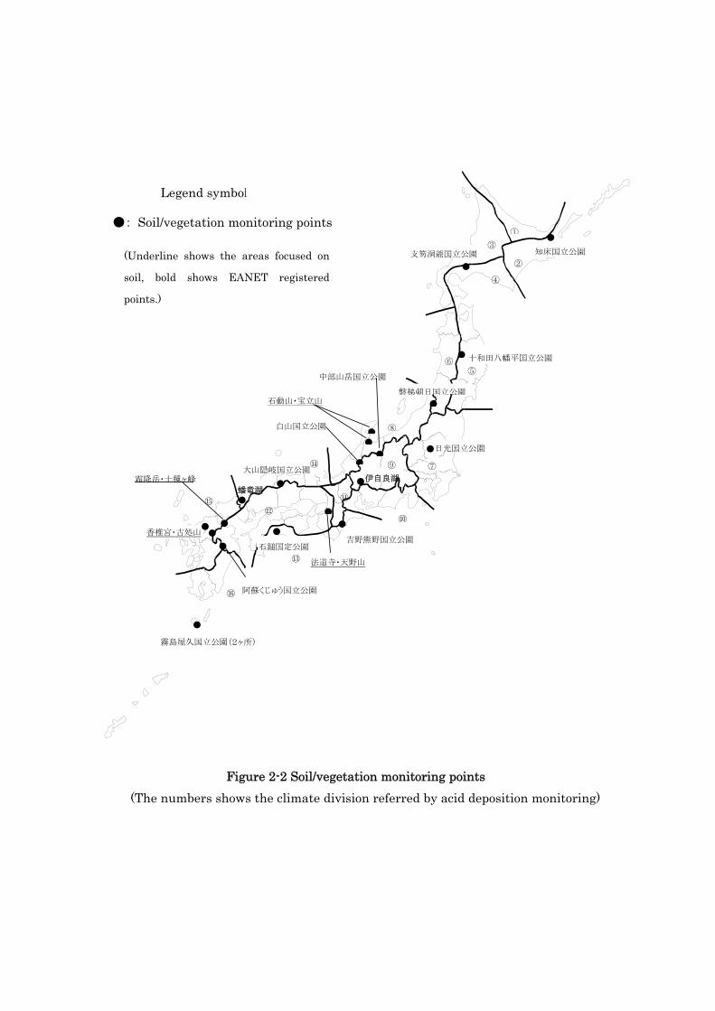
（３） Soil/vegetation monitoring

The soil/vegetation monitoring was conducted at total 25 points in 19 areas which were divided into 3 areas. First one was the area mainly focused on the influence to woods, which were mostly natural forests in mountain region which was thought to be affected by external irreversibility. The second one was the area mainly focused on the influence to soil, which were sensible against acid deposition. The third one was the area focused on the influence to land water, which was important to see the influence to land water (refer to table 2-2 for the list of the areas and figure 2-2 for the points distribution). The monitoring was conducted as follows based on “Soil/vegetation monitoring measuring handbook (1998)” and EANET technical manual.

① Forest monitoring The general survey to forests (per trees (name, breast high diameter, and height)) was

conducted once per 5 years, and the declining survey to woods (declination level, records and presumption by pictures) was conducted once a year.

② Soil monitoring

1 It is written as “NOX*” because peroxyacetyl nitrate and a part of nitric acids as well as besides NOX

（NO and NO2）are to be measured for analysis. Main elements of NOx at the at the measurement points in urban areas are considered NO and NO2, therefore, we count the value subtracting NOx from NO as NO2 measured value. 2 To be precise, the particulate materials collected with sizing devices of which trapping efficiency against particles with 10μm diameter (aerodynamic diameter) is 50%.

14

The following items were analyzed with the surface (0－10cm) and next layer (10－20cm) of soil. It was conducted once per 5 years.

●Required item: moisture content, pH (H2O）,pH (KCl), exchangeable base (Ca、Mg、Na、K), exchangeable acid degree, effective cation ion exchangeable content (ECEC), exchangeable AL and H, contained amount of carbonic acid (only in limestone soil).

● Selected items: overall nitrogen content, overall carbon content, phosphoric acid availability, sulfur ion, soil density, soil hardness.

15

Name Prefecture Category Wet period NOx SO2 O3 PM10 PM2.5 filter pack WD/WS Rain temp/humid radiation EANET

１ Rishiri

Hokkaido

Remote ○ Daily ○ ○ ○ ○ ○ ○ ○ ○ ○ ○ ○

２ Sapporo Urban ○ Weekly ○ ○ ○

３ Ochiishi Remote ○ Daily ○ ○ ○ ○ ○ ○ ○ ○ ○ ○

４ Tappi Aomori Remote ○ Daily ○ ○ ○ ○ ○ ○ ○ ○ ○ ○

５ Hachimantai Iwate Rural ○ Daily ○ ○

６ Nonodake Miyagi Rural ○ Daily ○ ○ ○ ○ ○

７ Obanazawa Yamagata Rural ○ Weekly ○ ○

８ Tsukuba Ibaraki Rural ○ Daily ○ ○ ○ ○ ○

９ Akagi Gunma Rural ○ Daily ○ ○ ○

10 Ogasawara Tokyo

Remote ○ Daily ○ ○ ○ ○ ○ ○ ○ ○ ○ ○

11 Tokyo＊ Urban ○ Daily ○ ○ ○

12 Sado-seki Niigata

Remote ○ Daily ○ ○ ○ ○ ○ ○ ○ ○ ○ ○

13 Maki Rural ○ Daily ○ ○ ○ ○ ○

14 Echizen Fukui Remote ○ Daily ○ ○

15 Happo Nagano Remote ○ Daily ○ ○ ○ ○ ○ ○ ○ ○ ○ ○

16 Ijira Gifu Rural ○ Weekly ○ ○ ○ ○ ○ ○ ○ ○ ○ ○

17 Inuyama Aichi Rural ○ Daily ○ ○ ○ ○ ○

18 Kyoto Kyoto Rural ○ Daily ○ ○ ○ ○ ○

19 Amagasaki Hyogo Urban ○ Daily ○ ○ ○ ○

20 Shionomisaki Wakayama Remote ○ Daily ○ ○

21 Oki Shimane

Remote ○ Daily ○ ○ ○ ○ ○ ○ ○ ○ ○ ○ ○

22 Banryu Urban ○ Weekly ○ ○ ○ ○ ○ ○ ○ ○ ○ ○

23 Kurahashi Hiroshima Rural ○ Daily ○ ○ ○ ○ ○

24 Yusuhara Kouchi Remote ○ Daily ○ ○ ○ ○ ○ ○ ○ ○ ○ ○

25 Chikugo Fukuoka Rural ○ Daily ○ ○ ○ ○ ○

26 Tsushima Nagasaki

Remote ○ Daily ○ ○ ○

27 Goto Remote ○ Daily ○ ○

28 Kujyu Oita Rural ○ Weekly ○ ○

29 Ebino Miyazaki Remote ○ Daily ○ ○ ○ ○ ○

30 Yaku Kagoshima Remote ○ Weekly ○ ○

31 Hedo Okinawa Remote ○ Daily ○ ○ ○ ○ ○ ○ ○ ○ ○ ○

Table 2-1 Measurement items at each observation points

＊：It started in 2007 at Tokyo. ＊：Atmosphere concentration and weather items by auto-measuring machines at Ochiishi cape was measured by Center for Global Environmental Research.

Table 2-2 Soil/vegetation monitoring points

Place Cat. Monitor

year＊２ Item Number of plot

Woods Soil Vegetation

1 Shiretoko National Park

（Hokkaido） Tree 2005 fir １２１

2 Shikotsu Toya National

Park（Hokkaido） Tree 2003 Betula ermanii １２１

3 Towada Hachimantai

National Park（Iwate） Tree 2004 Abies mariesii １２１

4 Bandai Asahi National

Park（Niigata） Tree 2007 beech １２１

5 Nikko National Park

（Tochigi） Tree 2003 beech １２１

6 Chubusangaku National

Park（Toyama） Tree 2005 beech １２１

7 Hakusan National Park

（Ishikawa） Tree 2006 beech １２１

8 Yoshino Kumano National

Park（Nara） Tree 2004 beech １２１

9 Daisen Oki National Park

（Tottori） Tree 2003 beech １２１

10 Ishizuchi Quasi-National Park（Kochi）

Tree 2004 beech １２１

11 Aso Kuju National Park

（Oita） Tree 2005 fagaceae １２１

12 Kirishima Yaku National

Park, Yaku Island

（Kagoshima）

Tree 2004 cedar １２１

13 Tree 2004 laurilignosa １２１

14 Sekidosan, Horyusan

（Ishikawa） Soil 2005

Red soil, brown

forest soil ２

２×

２２×１

15 Houdouji, Amanosan

（Osaka） Soil 2007

Yellow soil, reddish

brown forest soil２

２×

２２×１

16 Shimofuridake,

Tokusagamine（Yamaguchi） Soil 2003

Yellow soil,

kuroboku soil ２

２×

２２×１

17 Kashiinomiya, Koshosan

（Fukuoka） Soil 2007

Reddish brown forest

soil, brown forest

soil

２２×

２２×１

18 around Ijirako（Gifu）

（Ijira, Yamato）＊１

water

2006

Ijira catchment

brown forest soil,

kuroboku soil

２２×

２２×１

19 around Banryuko（Shimane）

（Banryuko）＊１

water

2006

Banryuko catchment

yellowish brown

forest soil, red

soil

２２×

２２×１

Note）＊１：Iwami Rinkuu Factory Park: Registered point with EANET ＊２：Year conducted general forest inventories and soil monitorings

知床国立公園 ●

● 十和田八幡平国立公園

日光国立公園

●

●

中部山岳国立公園

●

法道寺・天野山

●

● ●

●

●

大山隠岐国立公園霜降岳・十種ヶ峰

蟠竜湖

香椎宮・古処山 ●

霧島屋久国立公園（２ヶ所）

Legend symbol

●： Soil/vegetation monitoring points

(Underline shows the areas focused on

soil, bold shows EANET registered

points.)

伊自良湖

●

●

●

①

② ③

④

⑤⑥

⑦

⑧

⑨

⑩

⑪

⑫

⑬

⑭

⑮

⑯

●

支笏洞爺国立公園

磐梯朝日国立公園

白山国立公園

石鎚国定公園

●

吉野熊野国立公園

●●

石動山・宝立山

● ●

阿蘇くじゅう国立公園

Figure 2-2 Soil/vegetation monitoring points (The numbers shows the climate division referred by acid deposition monitoring)

（４）Land water monitoring Land water monitoring was conducted at 11 points which were selected in consideration of the high sensibility against acid deposition, small artificial pollution, and area balance on the basis of “Land water monitoring hand book (February in 2005)” (refer to table 2-3 for the list of the observation points and figure 2-3 for the distribution). The measurement items are following.

① Measurement items for water quality survey 4 times per year: water temperature, pH, electric conductivity, alkali level, NH4+, Ca2+ , Ｍｇ2+、Na+, K+, SO42-, NO3-, Cl-, Chl-a, DO (dissolved oxygen)

More than once a year: NO2-, PO43-, DOC, transparency, water color ② Measurement items for bottom sediment survey (once per 5 years) : SO42-、NO3-、

Table 2-3 List of lakes for land water monitoring

Name Prefecture

year of monitoring

of sediment

（once five years）

EANET

site

１ Imagamioike Yamagata 2005

２ Karikomiko Tochigi 2006

３ Sankyoike Niigata 2003

４ Ohatakeike Ishikawa 2007

５ Yashagaike Fukui 2006

６ Futagoike Nagano 2004

７ Ijirako Gifu 2006 ○

８ Sawanoike Kyoto 2003

９ Banryuko Shimane 2007 ○

10 Yamanokuchi-dam Yamaguchi 2004

11 Nagatomiike Kagawa 2007

In the survey, the samples were collected and analyzed at the local governments concerned, and summarized at Acid Deposition and Oxidant Research Center (including the data checking by the experts at the center and outside specialists). After that, the data was fixed through the inspection at acid deposition investigation meeting (atmosphere and ecosystem committee).

Also, as one of the actions for the Quality Assurance and Quality Control (QA/QC), we sent the precipitation, filter papers of filter pack, simulated samples of land water and soil samples to each laboratory. We conducted the comparative investigations

about the analyses (laboratory comparative investigations) and conducted the field surveys about the condition of the ambient surroundings and storage situation of the devices. The next chapter shows the monitoring results (including QA/QC).

●

●●

●

●

●

●

●

●

●

●

●

●

●

●

●

●

●

刈込湖

双子池

沢の池

大畠池

夜叉ケ池

伊自良湖

蟠竜湖

山居池●

今神御池

●

●

陸水モニタリング地点

●

●

●

●●

●

● ●

永富池

山の口ダム

Figure 2-3 Land water monitoring points

3．Monitoring

3.1 Acid Deposition Monitoring 3.1.1 Wet Deposition Monitoring

(1) Trends of the annual mean in wet deposition The wet deposition monitoring survey for 5 years from 2003 through 2007 has been carried out and

clarified the chemical compositions in wet deposition. The obtained data by conducting continually

collection and chemical analysis of precipitation samples were collected and comparison between sites

was performed. The percentage of the sites which satisfied data completeness criteria for each year

were 90% (27/30), 67% (20/30), 70% (21/30), 80% (24/30) and 90% (28/31) in 2003, 2004, 2005,

2006 and 2007 respectively. The numbers of monitoring sites from 2003 through 2006 were 30. In

2007, they were 32 sites, because Tokyo site was newly established in 2007

① Precipitation Amount

The annual precipitation amounts at each monitoring site ranged from 626 mm y-1 (Ochiishi in 2004) to 5123mm y-1 (Yakushima in 2004). Among the sites, the means of precipitation amount for 5 years at Yakushima (3831mm y-1), Ebino (3117mm y-1) and Yusuhara (2949mm y-1) were much and those at Ochiishi (830mm y-1), Rishiri (961mm y-1) and Sapporo (1018mm y-1) were little than other sites. Then, the tendencies of precipitation amounts were much at the Pacific Ocean side in Shikoku and Kyushu and those in Hokkaido were little. Moreover, about the variations for five years, an increase or a decrease tendency was not remarkable at every site.

② pH value

The annual mean pH value and the mean pH value for 5 years were shown in Fig .3.1.1. The annual mean pH value at each monitoring site ranged from pH 4.40 (Ijira in 2003) to pH 5.04 (Ogasawara in 2003). Recently, pH value at Rishiri, Sapporo, Goto were becoming low level. The mean pH value for 5 years ranged from pH4.51 (Ijira) to pH 4.95 (Ogasawara), while the overall mean was pH4.68. So, the precipitation in Japan has been still acidifying. Among the sites, the means of pH value at Ogasawara (pH 4.95), Hedo (pH 4.92) and Happo (pH 4.85) were little higher, and those at Ijira (pH4.51), Echizen-misaki (pH4.52) and Niigata-maki (pH4.56) were little lower.

③ Concentrations and deposition amounts of major ion components pH value is determined by the balance between acids and bases. In the case of wet

deposition, sulfuric acid and nitric acid are considered as acids, and gaseous ammonia and basic calcium compounds are considered as base constituents. Therefore, in precipitation, nss-SO4

2- and NO3

- in precipitation can be considered as acidification indexes, NH4+ and nss-Ca2+ can be

regarded as indexes which control the acidification. Moreover, each wet deposition amount of ion components can serve as effective information, in order to evaluate long-term effects on the ecosystem. The outline of concentrations and deposition amounts of these four main ions components and hydrogen-ion were shown in table.

Data completeness criteria for each site were set up and the data that satisfy the criteria were used for the calculation of monthly and annual means. The data completeness criteria used this report were as follows;

①Percent total precipitation should be 80% or more and percent precipitation coverage length should be 80%

or more.

②Contribution of sea salts is 75% or less.

Figure 3-1-1 Annual mean pH value

Chikugo-ogori4.85/ 4.83/ **/ 4.49/ 4.82/ 4.69

Rishiri 4.85/ 4.86/ 4.73/ 4.66/ 4.59/ 4.71

Sapporo 4.76/ **/ 4.70/ 4.54/ 4.57/ 4.64

Tsukuba 4.61/ 4.64/ 4.56/ 4.89/ 4.71/ 4.68

Tokyo-/ -/ -/ -/ 4.77/ 4.77

Inuyama 4.63/ **/ 4.50/ 4.57/ 4.64/ 4.59

Kyoto-yawata 4.67/ 4.84/ **/ **/ 4.60/ 4.70

Amagasaki 4.71/ 4.85/ 4.56/ 4.57/ 4.63/ 4.66

Shiono-misaki 4.74/ **/ **/ 4.62/ 4.54/ 4.63 Kurahashijima 4.48/ 4.63/ 4.52/ 4.64/ 4.55/ 4.57

Oita-kuju 4.59/ 4.70/ 4.58/ 4.74/ 4.79/ 4.67

Yakushima 4.67/ 4.78/ **/ **/ **/ 4.73

Ogasawara 5.04/ 5.02/ 4.84/ **/ 4.99/ 4.95

Tsushima 4.83/ **/ **/ **/ **/ 4.83

Oki 4.80/ 4.76/ 4.55/ 4.69/ 4.69/ 4.70

Echizen-misaki 4.54/ **/ 4.49/ 4.57/ 4.48/ 4.52

Happo 4.90/ **/ 4.78/ 4.96/ 4.78/ 4.85

Obanazawa 4.72/ 4.65/ 4.65/ 4.83/ 4.72/ 4.71

Tappi **/ **/ **/ 4.60/ 4.58/ 4.59

Hachimantai4.75/ 4.70/ 4.75/ **/ 4.81/ 4.75Ijira 4.40/ 4.65/ **/ 4.46/ 4.54/ 4.51

Yusuhara 4.76/ 4.92/ 4.67/ 4.83/ 4.78/ 4.80

Hedo 4.83/ **/ 4.88/ 4.95/ 4.98/ 4.92

Banryu 4.65/ 4.67/ 4.55/ 4.64/ 4.53/ 4.61

Niigata-maki 4.60/ 4.65/ 4.47/ 4.61/ 4.48/ 4.56

Ebino **/ 4.82/ 4.59/ 4.69/ **/ 4.70

Sado-seki **/ **/ 4.59/ 4.65/ 4.51/ 4.58

Akagi 4.59/ **/ **/ **/ 4.83/ 4.70

－：not measured

**：Data do not satisfy criteria for completeness Notes: Weighted averages for precipitation amounts are calculated

2003FY/ 2004FY/ 2005FY/ 2006FY/ 2007FY/ Average for five years

Ochiishi 4.88/ 4.70/ 4.82/ 4.86/ 4.79/ 4.81

Nonodake 4.77/ 4.75/ 4.54/ 4.92/ 4.70/ 4.74

Goto 4.82/ 4.90/ **/ 4.62/ 4.64/ 4.73

Table 3-1-1 Concentrations and deposition of main ion components in precipitation

Ion

components Concentration Deposition

nss-SO４2-

Range：4.1（2004, Ogasawara）～

26.6μmol L-1（2006, Chikugo-ogori、

2007, Goto）

Mean：13.8μmol L-1

Chikugo-ogori and Echizen-misaki

were high, and Ogasawara, Yusuhara,

and Hedo were low level


67.5mmol m-2 y-1（2006,

Chikugo-ogori）

Yakushima, Ijira, and Ebino were large, and Ochiishi and Ogasawara were small amoumt

NO3- Range：3.2（2005, Ogasawara）～

28.8μmol L-1（2007, Banryu）


Tappi, Sado-seki, and Echizen-misaki

were high, and Ogasawara, Yusuhara,

and Ebino were low level

Range：4.8（2004, Ogasawara）～68.0

mmol m-2 y-1（2006, Ijira）

Ijira, Yakushima and Echizen-misaki

were large, and Ogasawara and Ochiishi

were small amount

NH４+


37.2μmol L-1（2006, Chikugo-ogori）


Tokyo, Chikugo-ogori, and Sapporo were high, and Ogasawara, Yusuhara, and Hedo were low level

Range：5.7（2004, Ogasawara）～94.2

mmol m-2 y-1（2006, Chikugo-ogori）

Chikugo-ogori and Ijira were large,

andOgasawara and Ochiishi were small

amount

nss-Ca2+ Range：0.8（2005, Ogasawara）～

11.0μmol L-1（2007, Chikugo-ogori）

Mean：3.3μmol L-1

Tappi, Chikugo-ogori, and Sado-seki

were high, and Ebino, Chikugo-ogori,

and Yusuhara were low level

Range： 1.7（2005, Ogasawara）～17.9

mmol m-2 y-1（2007, Chikugo-ogori）

Chikugo-ogori and Happo were large,

and Ochiishi, Ogasawara, and Rishiri

were small amount

H+ Range：9.1（2004, Ogasawara）～

39.7μmol L-1（2004, Ijira）


Ijira and Echizen-misaki were high,

and Ogasawara and Hedo were low

level

Range： 10.8（2004, Ochiichi）～115

mmol m-2 y-1（2004, Ijira）

Ijira and Yakushima were large, and

Ochiishi, Ogasawara, and Rishiri were

small amount

(2) Seasonal variation of wet deposition In order to evaluation of seasonal fluctuation of wet deposition in each area, at first, 31

monitoring sites were classified into seven areas, Hokkaido, the Sea of Japan side in central and northern Honshu island, the Pacific Ocean side, the Inland Sea of Japan side, San-in, the East China Sea side, and Southwest islands. And then, the analysis on seasonal fluctuation of deposition amounts of each ion components were carried out for every area. Seasonal fluctuations about deposition amount, concentration, and precipitation amount of nss-SO4

2- and NO3

- which were indexes which contribute to acidification of precipitation, were shown in Fig.3-1-2 and Fig.3-1-3, respectively.

There were most precipitation in July in the Sea of Japan side in central and northern Honshu island, the Pacific Ocean side, the Inland Sea of Japan side, San-in, and the East China Sea side and was most precipitation in June on Southwest islands, because the rainy season has affected these area considerably. The other hand, there was most precipitation amount in September in Hokkaido because of the influence of typhoons.

The nss-SO42- concentrations have tended to become high from winter to spring in area

except Hokkaido. Moreover, NO3- concentrations have trended to become high from winter to

spring in area except Southwest islands. On a national scale, concentrations of nss-SO42- and NO3- increased generally in the

periods from winter to spring months whereas nss- SO42- in Hokkaido and NO3- in Southwest islands did not show clear seasonality as the other sites. The deposition showed a steep increase from late autumn to spring in the Sea of Japan side in central and northern Honshu island and San-in. This phenomenon is interpreted as indicating that increasing amounts of acids and its precursors are injected into the atmosphere during this period and suggesting continental pollutants are transported over these regions. In contrast, the deposition in the Pacific Ocean side, the Inland Sea of Japan side, and the East China Sea side had a maximum in July when the precipitation amount peaked in a year. Minimum deposition took place in winter months in the Pacific Ocean side and the Inland Sea of Japan side. In Hokkaido, deposition of nss-SO4

2- and NO3

- was likely to be lower than that in the other regions throughout the year. Concentration and deposition of NH4

+ had similar seasonality to those of NO3-, which implies these two

species followed a common atmospheric process. Non-sea-salt calcium ion showed the maximum in the concentration and deposition in spring time in all the regions except Southwest islands which had a second maximum in this season. This nation-wide seasonality suggested Kosa, or Asian dust, had a significant influence on precipitation chemistry in Japan.

Hydrogen ion concentration showed the maximum in winter in the regions of the Sea of Japan side in central and northern Honshu island, San-in, the East China Sea side, and Southwest islands although no apparent seasonality was noted in Hokkaido, the Pacific Ocean side, and the

Inland Sea of Japan side. The deposition was largest in winter time in the Sea of Japan side in central and northern Honshu island and San-in while the maximum deposition occurred in July in

the Pacific Ocean side, the Inland Sea of Japan side, and the East China Sea side.

Figure 3-1-2 Regional differences of seasonal variation of nss-SO42- concentration and deposition

(2003-2007)

0

200

400

600

0

25

50

75

100

4 5 6 7 8 9 10 11 12 1 2 3

Pre

cipi

tatio

n am

ount

／m

m

Dep

ositi

on ／

10m

mol

m-2

Con

cent

ratio

n ／μm

ol L

-1

Hokkaido

Precipitation amount Deposition Concentration

0

200

400

600

0

25

50

75

100

4 5 6 7 8 9 10 11 12 1 2 3

Pre

cipi

tatio

n am

ount

／m

m

Dep

ositi

on ／

10m

mol

m-2

Con

cent

ratio

n ／μm

ol L

-1

The Sea of Japan side in central and northern

Honshu Island


0

200

400

600

0

25

50

75

100

4 5 6 7 8 9 10 11 12 1 2 3

Pre

cipi

tatio

n am

ount

／m

m

Dep

ositi

on ／

10m

mol

m-2

Con

cent

ratio

n ／μm

ol L

-1

The Pacific Ocean side


0

200

400

600

0

25

50

75

100

4 5 6 7 8 9 10 11 12 1 2 3

Pre

cipi

tatio

n am

ount

／m

m

Dep

ositi

on ／

10m

mol

m-2

Con

cent

ratio

n ／μm

ol L

-1 The Inland Sea of Japan side


0

200

400

600

0

25

50

75

100

4 5 6 7 8 9 10 11 12 1 2 3

Pre

cipi

tatio

n am

ount

／m

m

Dep

ositi

on ／

10m

mol

m-2

Con

cent

ratio

n ／μm

ol L

-1

San-in


0

200

400

600

0

25

50

75

100

4 5 6 7 8 9 10 11 12 1 2 3

Pre

cipi

tatio

n am

ount

／m

m

Dep

ositi

on ／

10m

mol

m-2

Con

cent

ratio

n ／μm

ol L

-1 The East China Sea side


0

200

400

600

0

25

50

75

100

4 5 6 7 8 9 10 11 12 1 2 3

Pre

cipi

tatio

n am

ount

／m

m

Dep

osi

tion

／10m

mol

m-2

Co

nce

ntr

atio

n ／μm

ol L

-1

Southwest Islands


Figure 3-1-3 Regional differences of seasonal variation of NO3- concentration and deposition

(2003-2007)

0

200

400

600

0

25

50

75

100

4 5 6 7 8 9 10 11 12 1 2 3

Pre

cipi

tatio

n am

ount

／m

m

Dep

ositi

on ／

10m

mol

m-2

Con

cent

ratio

n ／μm

ol L

-1

Hokkaido


0

200

400

600

0

25

50

75

100

4 5 6 7 8 9 10 11 12 1 2 3

Pre

cipi

tatio

n am

ount

／m

m

Dep

ositi

on ／

10m

mol

m-2

Con

cent

ratio

n ／μm

ol L

-1

The Sea of Japan side in central and northern

Honshu Island


0

200

400

600

0

25

50

75

100

4 5 6 7 8 9 10 11 12 1 2 3

Pre

cipi

tatio

n am

ount

／m

m

Dep

ositi

on ／

10m

mol

m-2

Con

cent

ratio

n ／μm

ol L

-1

The Pacific Ocean side


0

200

400

600

0

25

50

75

100

4 5 6 7 8 9 10 11 12 1 2 3

Pre

cipi

tatio

n am

ount

／m

m

Dep

ositi

on ／

10m

mol

m-2

Con

cent

ratio

n ／μm

ol L

-1

The Inland Sea of Japan side


0

200

400

600

0

25

50

75

100

4 5 6 7 8 9 10 11 12 1 2 3

Pre

cipi

tatio

n am

ount

／m

m

Dep

ositi

on ／

10m

mol

m-2

Con

cent

ratio

n ／μm

ol L

-1

San-in


0

200

400

600

0

25

50

75

100

4 5 6 7 8 9 10 11 12 1 2 3

Pre

cipi

tatio

n am

ount

／m

m

Dep

ositi

on ／

10m

mol

m-2

Con

cent

ratio

n ／μm

ol L

-1

The East China Sea side


0

200

400

600

0

25

50

75

100

4 5 6 7 8 9 10 11 12 1 2 3

Pre

cipi

tatio

n am

ount

／m

m

Dep

ositi

on ／

10m

mol

m-2

Con

cent

ratio

n ／μm

ol L

-1

Southwest Islands


(3) Long-term trends of wet deposition

In order to assess long-term trends of wet deposition, annual variations of the national medians

for the annual means of rainfall amount, concentrations and deposition of major ions were explored

for the sites with more than ten year valid measurements in the period from FY1991 to FY2007.

The medians for the rainfall amount and the concentrations are summarized in Fig. 3.1.4. The

precipitation amount fluctuated in FY1990s and approached to a plateau in FY2000s. Deposition of

nss-SO42- was invariant throughout the period in spite of some variations. Nitrate deposition

increased in the middle of 1990s and changed by leveling off thereafter. Ammonium and nss-Ca2+

deposition leveled off during the period with some slight fluctuation. Deposition of H+ was likely to

increase from the middle of FY1990s to FY2000 and then showed some fluctuations.

Figure 3-1-4 Trends in annual median of precipitation amounts

and deposition of ion components The annual trends of the medians for pH and concentrations of major ions are illustrated in Fig.

3.1.5. Generally, pH has been rather invariant with some fluctuations. Concentration of nss-SO42-

had a decreasing trend up to FY1999, increased in FY2000, and eventually approached a plateau

whereas that of NO3- has been invariant until FY2004 with a fluctuating trend and increased after

FY2005. Ammonium concentration has been generally unvarying with occasional fluctuation and

nss-Ca2+ concentration fluctuated in such a manner as it was elevated in FY2000 whereas lowered

in FY2003 and FY2004.

0

10

20

30

40

1991

1992

1993

1994

1995

1996

1997

1998

1999

2000

2001

2002

2003

2004

2005

2006

2007

NH

4+ 沈着

量/m

mol

m-2

y-1 NH4+沈着量

0

10

20

30

1991

1992

1993

1994

1995

1996

1997

1998

1999

2000

2001

2002

2003

2004

2005

2006

2007

nss-

SO42-

沈着

量/m

mol

m-2

y-1

nss-SO42-沈着量

0

5

10

1991

1992

1993

1994

1995

1996

1997

1998

1999

2000

2001

2002

2003

2004

2005

2006

2007

nss-

Ca2

+ 沈着

量/m

mol

m-2

y-1 nss-Ca2+沈着量

0

10

20

30

40

1991

1992

1993

1994

1995

1996

1997

1998

1999

2000

2001

2002

2003

2004

2005

2006

2007

H+ 沈

着量

/mm

ol m

-2 y

-1

H+沈着量

0

10

20

30

1991

1992

1993

1994

1995

1996

1997

1998

1999

2000

2001

2002

2003

2004

2005

2006

2007

NO

3- 沈着

量/m

mol

m-2

y-1

NO3-沈着量

0

500

1000

1500

2000

2500

1991

1992

1993

1994

1995

1996

1997

1998

1999

2000

2001

2002

2003

2004

2005

2006

2007

降水

量/m

m

降水量

0

10

20

30

40

1991

1992

1993

1994

1995

1996

1997

1998

1999

2000

2001

2002

2003

2004

2005

2006

2007

NH

4+ dep

osit

ion

/ mm

ol m

-2 y

-1

NH4+deposition

0

10

20

30

1991

1992

1993

1994

1995

1996

1997

1998

1999

2000

2001

2002

2003

2004

2005

2006

2007

nss-

SO42-

depo

siti

on /m

mol

m-2

y-

1

nss-SO42-deposition

0

5

10

1991

1992

1993

1994

1995

1996

1997

1998

1999

2000

2001

2002

2003

2004

2005

2006

2007ns

s-C

a2+ d

epos

itio

n / m

mol

m-2

y-1 nss-Ca2+deposition

0

10

20

30

40

1991

1992

1993

1994

1995

1996

1997

1998

1999

2000

2001

2002

2003

2004

2005

2006

2007

H+ d

epos

itio

n / m

mol

m-2

y-1

H+deposition

0

10

20

30

1991

1992

1993

1994

1995

1996

1997

1998

1999

2000

2001

2002

2003

2004

2005

2006

2007

NO

3- dep

osit

ion

/ mm

ol m

-2 y

-1

NO3-deposition

0

500

1000

1500

2000

2500

1991

1992

1993

1994

1995

1996

1997

1998

1999

2000

2001

2002

2003

2004

2005

2006

2007

Prec

ipit

atio

n a

mou

nt /

mm

Precipitation

Figure 3-1-5 Trends in annual median of pH value

and concentration of ion components

(4) Quality Assurance / Quality Control

To obtain comparable, high quality monitoring data, each participating country is required to

carry out acid deposition monitoring using common methodologies as specified in the Guidelines

for Acid Deposition Monitoring in East Asia, Technical Documents on Wet Deposition

Monitoring in East Asia. And the inter-laboratory comparison project (round robin analysis

survey) was conducted among the analytical laboratories in participating countries of the Acid

Deposition Monitoring Network in East Asia (EANET). Some of Japan domestic center or

analytical agency participate WMO or EMEP inter-laboratory comparison, and keep analytical

quality. Acid Deposition and Oxidant Research Center also direct site audit to monitoring site and

analytical laboratory.

1) Inter-laboratory comparison project of wet deposition measurements

The objectives of the project are, through the evaluation of analytical results, analytical

equipment and its operating condition and other practices,

i) to recognize the analytical precision and accuracy of the measurement in each

participating laboratory,

ii) to give an opportunity to improve the quality of the analysis on wet deposition

iii) to improve reliability of analytical data through the assessment of suitable analytical

methods and techniques.

4.2

4.4

4.6

4.8

5

5.2

5.4

199

1199

2199

3

199

4199

5199

6

199

7199

8199

9

200

0200

1200

2

200

3200

4200

5

200

6200

7

pH

pH

0

5

10

15

20

25

1991

1992

1993

1994

1995

1996

1997

1998

1999

2000

2001

2002

2003

2004

2005

2006

2007ns

s-SO

42-co

ncen

trat

ion

/μm

ol L

-1

nss-SO42-concentration

0

5

10

15

20

25

1991

1992

1993

1994

1995

1996

1997

1998

1999

2000

2001

2002

2003

2004

2005

2006

2007

NO

3- conc

entr

atio

n / μ

mol

L-1

NO3-concentration

0

5

10

15

20

25

1991

1992

1993

1994

1995

1996

1997

1998

1999

2000

2001

2002

2003

2004

2005

2006

2007

NH

4+ con

cent

ratio

n / μ

mol

L-1

NH4+concentration

0

2

4

6

8

1991

1992

1993

1994

1995

1996

1997

1998

1999

2000

2001

2002

2003

2004

2005

2006

2007ns

s-C

a2+ c

once

ntra

tion

/ μm

ol L

-1

nss-Ca2+concentration

ADORC provide two practice rain sample (high concentration and low concentration) to

monitoring center or analytical agency, these analytical data will submitted to ADORC, and

assessed by Data Quality Objectives (DQOs : with in ±15%)*.

In this investigate term, analytical data quality keep 99% of DQOs at high concentration

samples, and 90% of DQOs at low concentration samples.

*(Flag E will be marked 15% to 30% of DQOs. Flag X will be marked over 30% of DQOs)

2) Site audit of monitoring stations

As part of the QA/QC, ADORC direct site audit to monitoring site and analytical laboratory.

EANET site is once two years, other domestic site is once three years. Site audit checked wet

sampler condition, surround blockade or source of pollution, collecting sample, and analytical

methods.

3.1.2 Dry Deposition Monitoring

(1) Trend of annual mean and seasonal variation in dry depostion

The outline of dry deposition monitoring for major monitoring parameter in 2003 to 2007,

was shown in Table 3-1-2. Moreover, temporal variations of monthly mean for SO2, O3 and PM10

and PM2.5 based on the five year estimates were shown in Figure 3-1-6, 3-1-7, and 3-1-8,

respectively. The other parameters were referring to the reference data.The annual value and monthly

value which were used for analysis were based on the datasets with data completeness of over 70%

(An automatic monitor method: one hour value, a filter pack method: two weeks value).

Major measurement parameters

① Automatic Monitor Method

SO2（12sites）、NOx*（11sites）、O3（21sites）、PM10（11sites）、PM2.5（3sites）

② Filter-pack Method

Concentration of particulate component (SO42-、NO3

-、NH4+、Ca2+）（11sites）

Concentration of gaseous component （HNO3、NH3）（11sites）

About SO42- in the particulate component, non-sea salt SO4

2- computed from Na+ concentration as an

index of a sea salt like wet deposition, was used for consideration.

Table 3-1-2 Results of main monitoring items

Monitoring Items Tendency of annual means and variations of monthly concentrations

SO2 Automatic

Monitor

・Range：<0.1ppb（2003, 2004, and 2007: Ogasawara）～1.2ppb（2005:

Yusuhara、2007: Banryu and Ebino）

Yusuhara,Ebino, and Banryu were high, and Ogasawara was low level.

Mean (2003-2007): 0.6ppb

The variations of monthly mean;

There were many sites where SO2 concentrations became high from the late

autumn to spring, and those concentrations rose greatly on the western Japan.

In Ogasawara, low concentration continued through every year. The high

concentrations from the late autumn to spring were considered to be the effect

of transboundary air pollution like the seasonal variation of the nss-SO42-

deposition described by 3.1.1 (2). NOx*

Automatic

Monitor

・Range：0.4ppb（2003, 2004, and 2007: Ogasawara）～4.2ppb（2003: Banryu）

Banryu, Ijira and Banryu were high, and Ogasawara was low level.

Mean (2003-2007) : 1.7ppb


The high concentrations in the western Japan or along the coast of japan sea

from the late autumn to spring were considered to be the effect of

transboundary air pollution like the seasonal variation of the NO3- deposition

described by 3.1.1 (2). The concentration at Ijira was low in winter, and

fluctuation of concentration at Rishiri, Ochiishi, Happo, and Hedo were small

through every year.

O3 Automatic

Monitor

・Range：19ppb（2005: Ijira）～60ppb（2004: Akagi、and Happo）

Happo and Akagi were high, and Ijira and Kyoto-yawata were low level

Mean (2003-2007): 39ppb


O3 concentration at all sites were high in spring and low in summer, moreover

in western Japan, high concentrations of O3 were appeared in autumn. O3

concentrations were high at Happo and Akagi where these height were higher

than the other sites through every year.

The high concentration in spring was considered to be the effect of transboundary air pollution.

PM10 Automatic

・Range：11μg m-3（2003: Ogasawara）～37μg m-3（2005: Hedo）

Hedo was high, and Ogasawara and Happo were low level

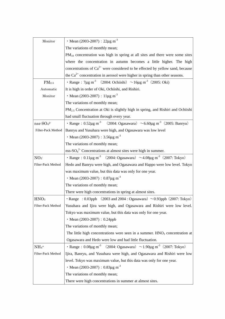
Monitor ・Mean (2003-2007)：22μg m-3


PM10 concentration was high in spring at all sites and there were some sites

where the concentration in autumn becomes a little higher. The high

concentrations of Ca2+ were considered to be effected by yellow sand, because

the Ca2+ concentration in aerosol were higher in spring than other seasons. PM2.5

Automatic

Monitor

・Range：7μg m-3 （2004: Ochiishi）～16μg m-3（2005: Oki)

It is high in order of Oki, Ochiishi, and Rishiri.

・Mean (2003-2007)：11μg m-3


PM2.5 Concentration at Oki is slightly high in spring, and Rishiri and Ochiishi

had small fluctuation through every year. nss-SO42- Filter-Pack Method

・Range：0.52μg m-3�（2004: Ogasawara）～6.60μg m-3（2005: Banryu）

Banryu and Yusuhara were high, and Ogasawara was low level

・Mean (2003-2007)：3.56μg m-3


nss-SO42- Concentrations at almost sites were high in summer.

NO3- Filter-Pack Method

・Range：0.11μg m-3 （2004: Ogasawara）～4.08μg m-3（2007: Tokyo）

Hedo and Banryu were high, and Ogasawara and Happo were low level. Tokyo

was maximum value, but this data was only for one year.

・Mean (2003-2007)：0.87μg m-3


There were high concentrations in spring at almost sites.

HNO3

Filter-Pack Method

・Range ：0.03ppb （2003 and 2004 : Ogasawara）～0.93ppb（2007: Tokyo）

Yusuhara and Ijira were high, and Ogasawara and Rishiri were low level.

Tokyo was maximum value, but this data was only for one year.

・Mean (2003-2007)：0.24ppb


The little high concentrations were seen in a summer. HNO3 concentration at

Ogasawara and Hedo were low and had little fluctuation.

NH4+ Filter-Pack Method

・Range：0.08μg m-3 （2004: Ogasawara）～1.90μg m-3（2007: Tokyo）

Ijira, Banryu, and Yusuhara were high, and Ogasawara and Rishiri were low

level. Tokyo was maximum value, but this data was only for one year.

・Mean (2003-2007)：0.83μg m-3


There were high concentrations in summer at almost sites.

NH3 Filter-Pack Method

・Range：0.18ppb （2003: Ogasawara）～5.64ppb（2007: Tokyo）

Ijira and Banryu were high, and Rishiri, Tappi, and Happo were low level.

Tokyo was maximum value, but this data was only for one year.

・Mean (2003-2007)：0.78ppb


The high concentrations from spring to summer were appeared at many sites.

Although Tokyo had only one year data, high concentration was continued.

Ca2+

Filter-Pack Method

・Range ：0.02μg m-3�（2004: Ogasawara）～0.57μg m-3（2007: Tokyo）

Hedo was high, and Ogasawara was low level. Tokyo was maximum value, but

this data was only for one year.

・Mean (2003-2007)：0.24μg m-3


The high concentrations were appeared at almost sites in spring, and the effect

of yellow sand was suggested.

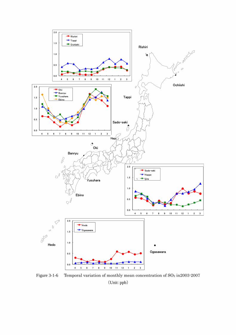
Figure 3-1-6 Temporal variation of monthly mean concentration of SO2 in2003-2007（Unit：ppb）

0.0

0.5

1.0

1.5

2.0

4 5 6 7 8 9 10 11 12 1 2 3

Rishiri

Tappi

Ochiishi

0.0

0.5

1.0

1.5

2.0

4 5 6 7 8 9 10 11 12 1 2 3

Oki

Banryu

Yusuhara

Ebino

0.0

0.5

1.0

1.5

2.0

4 5 6 7 8 9 10 11 12 1 2 3

Sado-seki

Happo

Ijira

0.0

0.5

1.0

1.5

2.0

4 5 6 7 8 9 10 11 12 1 2 3

Hedo

Ogasawara

Rishiri

Ogasawara

Oki

Happo

Tappi

Ochiishi

Ijira

Yusuhara

Hedo

Banryu

Ebino

Sado-seki

Figure 3-1-7 Temporal variation of monthly mean concentration of O3 in2003-2007 (Unit:ppb)

Rishiri

Nonodake

Tsukuba

Inuyama

Kyoto-yawata

Kurahashizima

Ogasawara

Oki Happo

Tappi

Ochiishi

Ijira

Yusuhara

Hedo

Banryu

Ebino

Sado-seki

Akagi

Niigata-maki

0

20

40

60

80

100

4 5 6 7 8 9 10 11 12 1 2 3

Rishiri

Tappi

Ochiishi

0

20

40

60

80

100

4 5 6 7 8 9 10 11 12 1 2 3

Nonodake

Tsukuba

Akagi

0

20

40

60

80

100

4 5 6 7 8 9 10 11 12 1 2 3

Sado-seki

Happo

Niigata-maki

0

20

40

60

80

100

4 5 6 7 8 9 10 11 12 1 2 3

I jira

Inuyama

Kyoto-yawata

0

20

40

60

80

100

4 5 6 7 8 9 10 11 12 1 2 3

Oki

Banryu

Kurahashizima

0

20

40

60

80

100

4 5 6 7 8 9 10 11 12 1 2 3

Yusuhara

Chikugo-ogori

Tsushima

Ebino

0

20

40

60

80

100

4 5 6 7 8 9 10 11 12 1 2 3

Hedo

Ogasawara

Figure 3-1-8 Temporal variation of monthly mean concentration of PM10 and PM2.5 in2003-2007

(Unit: μg m-3）

Rishiri

Ogasawara

Oki

Happo

Tappi

Ijira

Yusuhara

Hedo

Banryu

Sado-seki

Ochiishi 0

10

20

30

40

50

4 5 6 7 8 9 10 11 12 1 2 3

Rishiri(PM10)

Rishiri(PM2.5)

Tappi

Ochiishi(PM10)

Ochiishi(PM2.5)

0

10

20

30

40

50

4 5 6 7 8 9 10 11 12 1 2 3

Oki(PM10)

Oki(PM2.5)

Banryu

Yusuhara

0

10

20

30

40

50

4 5 6 7 8 9 10 11 12 1 2 3

Sado-seki

Happo

Ijira

0

10

20

30

40

50

4 5 6 7 8 9 10 11 12 1 2 3

Hedo

Ogasawara

(2) Long-term trends of dry deposition

・SO2

During the period from 1998 to 2007, temporal variations of SO2 concentration were illustrated

for sites with valid data for more than six years in Figure 3-1-9.

SO2 concentrations in remote sites were 1.0ppb or less in concentration in general. In it, the

concentration in Yusuhara was high and these in Ogasawara and Rishiri located far from the

continent were low in this period. In remote sites along the coast of Japan Sea, SO2 concentrations

were likely to decreased from the west side in order of Oki, Sado-Seki, Tappi, and Rishiri, and it

was suggested that continental source contribution was larger as the site position was nearer to the

continent. On the other hand, in non-remote sites including Ebino near Sakurajima an active

volcano, the concentration in Ebino and Banryu were same level that were higher than in Ijira in

this period.

In Sado-seki, Happo, Ijira, and Yusuhara, SO2 concentrations were higher in 2000 and 2001,

which would be attributable to the volcanic SO2 originating the eruption of Mount Oyama on

Miyake Island in August, 2000. In consideration of this effect, in recent years, some increasing

trends on the concentration with fluctuations were noted in Tappi, Oki, Yusuhara, and Hedo, and the decreasing trend was suggested in Ijira.

［a］：Remote sites ［b］：Non-remote sites

Figure 3-1-9 Trends in annual SO2 concentration

・NOx*

During the period from 1998 to 2007, temporal variations of NOX* concentration were

illustrated for sites with valid data for more than six years in Figure 3-1-10.

NOX* concentration in Ijira and Banryu in non-remote site were higher than other remote sites.

In remote site, the concentration in Ogasawara and Hedo were low and that in Happo was high.

About long-term trend, decreasing trends on the concentration were noted in Yusuhara, Ijira,and

0.0

0.2

0.4

0.6

0.8

1.0

1.2

1.4

1998

1999

2000

2001

2002

2003

2004

2005

2006

2007

SO

2濃

度/ p

pb

伊自良湖

蟠竜湖

えびの

0.0

0.2

0.4

0.6

0.8

1.0

1.2

1.4

1998

1999

2000

2001

2002

2003

2004

2005

2006

2007

SO

2濃

度/ p

pb

利尻

竜飛岬

佐渡関岬

八方尾根

隠岐

檮原

辺戸岬

小笠原

Banryu, and the stable trends were suggested in other sites.


Figure 3-1-10 Trends in annual NOX * concentration

・PM10

During the period from 1999 to 2007, temporal variations of PM10 concentration were

illustrated for sites with valid data for more than five years in Figure 3-1-11.

In remote site, the concentration in Ogasawara and Happo were low and that in Hedo near from

the continent was high. Moreover, in remote sites along the coast of the Japan Sea, In remote sites

in the Sea of Japan side, PM10 concentrations were likely to decreased from the west side in order

of Oki, Sado-Seki, Tappi, and Rishiri, and it was suggested that continental source contribution

was larger as the site position was nearer to the continent like SO2 concentration. In non-remote

sites, PM10 concentration in Banryu was higher than in Ijira in this period. The long-term trends

were stable in almost sites except Hedo.


Figure 3-1-11 Trends in annual PM10 concentration

0

1

2

3

4

5

1998

1999

2000

2001

2002

2003

2004

2005

2006

2007

NO

x / p

pb

伊自良湖

蟠竜湖

0

1

2

3

4

5

1998

1999

2000

2001

2002

2003

2004

2005

2006

2007

NO

x / p

pb

利尻

竜飛岬

佐渡関岬

八方尾根

隠岐

檮原

辺戸岬

小笠原

0

10

20

30

40

50

1999

2000

2001

2002

2003

2004

2005

2006

2007

PM

10濃

度/ μ

g m

-3

伊自良湖

蟠竜湖

0

10

20

30

40

50

1999

2000

2001

2002

2003

2004

2005

2006

2007

PM

10濃

度/ μ

g m

-3

利尻

竜飛岬

佐渡関岬

八方尾根

隠岐

檮原

辺戸岬

小笠原

・O3

Monitoring sites where the valid data was obtained from 1998 in 2007 for seven years or more

were classified into the remote (Rishiri, Tappi, Ogasawara, Sado-seki, Oki, Yusuhara, Tsushima,

and Hedo), the non-remote (Ijira, Kyoto-yawata, Banryu, Kurahashijima, Chikugo-ogori), the

alpine remote (happo), and alpine non-remote (Akagi). Trends of annual mean concentration of O3

in 2000 to 2007 when the valid data was obtained at 12 or more sites were shown in Figure 3-1-12

and 3-1-13.

Since annual mean concentratios for every classified area were high in order of the alpine, the

remote, and the effect from the stratosphere in the alpine were larger than those from the ground

level and the disappearance reaction of O3 by NO in non remote had arisen rather than the remote.

Moreover, O3 annual mean concentration ia remote, non-remote, alpine remote, and all sites

were tended to increase.At the remote sites, O3 concentrations were likely to decrease in order of

the mountainous sites, the Sea of Japan side, and the Pacific Ocean side.

Figure 3-1-12 Trends in annual PM10 Figure 3-1-13 Trends in annual O3

concentration every regions concentration

0

10

20

30

40

50

60

70

1998

1999

2000

2001

2002

2003

2004

2005

2006

2007

O3濃

度/ p

pb

利尻

竜飛岬

佐渡関岬

八方尾根

隠岐

檮原

辺戸岬

小笠原

対馬

0

10

20

30

40

50

60

70

2000

2001

2002

2003

2004

2005

2006

2007

O3濃

度/ p

pb

全地点

遠隔

非遠隔

高山遠隔

高山非遠隔

(3) Estimation of Dry Deposition

In 10 sites (EANET sites except Tokyo and Ochiishi) which monitored the atmosphere using

the filter-pack method in the 2003 to 2007, the dry deposition (gaseous substance: SO2, HNO3,

NH3, ion components in particulate matters: nss-SO42-, NO3

-, NH4+) at each site was estimated, and

the results were shown in Table 3-1-3. The estimation method was made into the presuming

method (the Inferential method) which searched from the product of the ingredient for the

concentration in the atmosphere and the deposition rate of the each component. The deposition rate

of each component was setting deposition surface to the forest and the grass field using the data of

meteorological elements based on the Matsuda's method.

Dry deposition amounts to the forest were much than those to grass field for either the gaseous

and particle matter. About the deposition of gaseous substances to the forest, SO2 depositions at

Banryu, Hedo, Sado-seki, and Tappi were larger, and those at Ijira and Rishiri were smaller. HNO3

depositions at Yusuhara, happo, Sado-seki, Banryu, and Tappi were larger, and that at Ogasawara

was small. Moreover, NH3 deposition showed large amount at Banryu. About the deposition of the

particulate matter to the forest, every depositoin at Tappi and Hedo were large, and those at

Ogasawara and Ijira were small. The concentration of gaseous and particulate matter at Tappi and

Sado-seki were not higher than other sites. But, there was a tendency for a deposition rate to

become large depending on an ingredient, so that wind velocity was large. As the results, the large

deposition amounts were estimated at both sites where had large wind velocity compared with the

other sites. There is a tendency for a deposition rate to become large depending on an ingredient, so

that wind velocity is large.

(4) Quality Assurance / Quality Control

Based on the 3rd Scientific Advisory Committee, inter-laboratory comparison for dry deposition

started since 2005. Impregnated filters which contain three ions, SO42-, Cl-, and NH4

+, were prepared

and distributed to the participating laboratories by the Network Center (NC). Most of the

laboratories participating in EANET activities joined this activity and submitted their analytical

results to NC. Obtained results for the amount of SO42-, Cl-, and NH4

+ on the distributed filters were

compared with the prepared values and statistically treated.

Submitted analytical data quality for low concentration sample were keep these quality, 83.3%

of DQOs at 1st project, 85.7% of DQOs at 2nd project, and 66.7% of DQOs at 3rd project.

In high concentration samples were keep these quality, 91.7% of DQOs at 1st project, 100%

of DQOs at 2nd project, and 95.2% of DQOs at 3rd project.

Table 3-1-3 Dry Deposition

SO2 HNO3 NH3 SO2 HNO3 NH3 nss-SO42- NO3

- NH4+ nss-SO4

2- NO3- NH4

+

Rish iri 2003 4.0 7.2 4.7 2.2 2.0 2.7 7.7 4.5 8.6 0.8 0.4 0.92004 4.1 5.1 5.2 2.1 1.4 3.0 7.1 4.6 6.5 0.6 0.4 0.62005 3.9 7.0 4.6 2.1 1.9 2.7 8.9 4.5 9.1 0.8 0.3 0.92006 4.3 4.9 4.5 2.3 1.3 2.3 7.2 3.9 7.3 0.7 0.3 0.72007 ** ** ** ** ** ** ** ** ** ** ** **

Tappi 2003 15.9 19.4 5.2 7.3 5.4 3.9 13.5 11.6 19.2 1.0 0.7 1.42004 16.9 21.2 5.2 7.2 5.9 3.5 17.9 14.0 19.3 1.1 0.7 1.32005 14.1 22.0 2.3 6.2 6.1 1.7 21.8 16.7 25.3 1.6 0.9 1.82006 16.6 16.7 2.8 8.0 4.7 2.1 19.1 16.2 22.7 1.4 0.9 1.72007 15.2 20.7 4.1 7.8 5.8 3.2 22.9 18.3 23.5 1.5 1.0 1.7

Ogasawara 2003 7.6 2.0 2.3 2.7 0.5 1.2 1.5 1.1 1.0 0.4 0.2 0.32004 7.6 2.3 3.4 3.3 0.6 2.0 0.5 0.3 0.4 0.1 0.1 0.12005 9.9 2.5 7.1 3.7 0.7 4.0 1.6 0.7 1.0 0.4 0.1 0.22006 ** ** ** ** ** ** ** ** ** ** ** **2007 1.9 2.6 5.1 0.7 0.7 2.8 4.3 1.9 3.0 0.7 0.3 0.5

Sade-seki 2003 12.5 18.3 3.3 5.4 5.0 2.4 10.1 6.5 8.3 0.7 0.4 0.72004 ** ** ** ** ** ** ** ** ** ** ** **2005 16.1 28.8 4.2 7.0 7.9 3.2 15.4 7.7 14.3 1.3 0.5 1.32006 20.7 23.2 4.4 8.1 6.4 3.2 12.7 7.8 12.0 1.0 0.5 1.12007 22.5 20.3 4.5 9.6 5.6 3.5 18.9 13.3 17.4 1.3 0.8 1.3

Happo 2003 11.8 21.8 6.8 5.5 6.1 3.1 8.7 3.2 10.9 0.8 0.2 1.22004 15.9 23.4 5.3 6.8 6.6 2.9 11.0 4.0 13.0 1.0 0.3 1.42005 16.5 14.9 6.9 7.4 4.2 3.7 12.3 3.5 14.2 1.2 0.2 1.62006 10.9 23.6 5.1 5.5 6.5 2.8 9.5 1.6 10.8 1.0 0.1 1.22007 10.6 24.5 4.2 5.1 6.8 2.3 9.7 1.8 12.0 1.0 0.2 1.3

I jira 2003 3.9 4.5 8.9 1.4 1.2 3.3 1.7 0.4 3.1 0.5 0.1 1.02004 4.2 7.0 8.5 1.6 1.9 3.5 2.5 0.6 3.7 0.9 0.2 1.32005 3.4 7.5 7.9 1.4 2.0 3.3 2.6 0.5 3.9 0.9 0.2 1.42006 3.0 6.6 7.6 1.3 1.8 3.2 2.3 0.5 3.4 0.9 0.1 1.42007 2.3 5.1 5.9 1.0 1.4 2.7 2.0 0.5 3.0 0.8 0.2 1.3

Oki 2003 12.0 7.2 5.0 5.4 2.0 3.2 11.5 5.7 8.6 1.1 0.4 0.92004 12.7 8.4 5.8 5.6 2.3 4.0 10.7 6.9 12.8 1.1 0.6 1.42005 15.8 16.4 5.5 6.7 4.5 3.9 17.5 8.9 19.8 2.0 0.7 2.42006 15.5 15.9 4.1 7.2 4.3 3.2 16.8 9.0 20.1 1.9 0.7 2.32007 ** ** ** ** ** ** ** ** ** ** ** **

Banryu 2003 18.5 12.7 10.3 8.2 3.5 6.1 8.3 4.3 8.1 1.0 0.4 0.92004 21.6 19.8 13.1 9.0 5.4 7.8 11.7 6.8 15.3 1.5 0.6 2.02005 16.9 23.0 8.3 8.1 6.3 5.3 14.4 8.0 19.4 2.1 0.7 2.72006 21.4 20.9 9.9 9.5 5.7 6.1 15.6 8.5 20.8 2.3 0.8 3.02007 21.2 21.2 8.8 9.5 5.8 5.5 15.6 8.2 20.1 2.0 0.8 2.7

Yusuhara 2003 11.7 16.7 5.4 5.8 4.6 3.0 8.3 2.8 10.3 1.4 0.4 1.72004 11.7 19.0 5.3 5.2 5.2 2.7 11.6 2.3 13.4 1.8 0.3 2.22005 12.3 25.5 3.6 6.4 7.2 2.2 11.9 2.7 15.0 2.5 0.4 3.12006 17.8 23.7 4.8 8.2 6.7 2.4 11.1 2.4 14.8 2.2 0.3 2.82007 17.5 25.3 7.3 8.5 7.1 3.5 12.5 2.5 15.5 2.3 0.4 3.0

Hedo 2003 21.1 8.9 5.0 9.0 2.4 3.9 16.3 17.4 16.7 1.4 1.2 1.42004 28.9 14.2 6.7 12.6 3.9 5.2 9.6 6.6 7.9 0.9 0.5 0.72005 17.1 11.4 5.9 7.5 3.2 4.8 26.0 14.9 22.0 2.4 1.0 2.02006 13.8 8.6 5.4 6.4 2.4 4.3 24.4 14.9 19.4 2.3 1.1 1.92007 12.4 12.0 7.9 5.6 3.3 6.2 26.2 14.3 24.2 2.2 1.0 2.3

**　Data was rejected because of less than 70% of valid data in the period

Site Year

Gaseous substance (mmol m-2 year-1) Particu late matter (mmol m-2 year-1)

Forest Grass f ie ld Forest Grass f ie ld

3.1.3 Synthetic consideration to acid deposition (1) Total Deposition

Total deposition of sulfur and nitrogen were calculated as the sum total value of these wet

depositions and dry depositions.

Wet deposition were used the actual measurement value shown at 3.1.1.

Dry deposition were used the value which computed from the weight average of the dry

deposition of a forest and a grassy field estimated at 3.1.2 (3) with a land use rate around about 1km

of monitoring site.

The distribution of the total deposition of sulfur and nitrogen were shown in Figure 3-1-14 and

3-1-15. The deposition of sulfur and nitrogen were corresponding to sulfur dioxide and nitrogen

oxide, respectively, which were the main causative agents of acid deposition.

In addition, the calculated periods were covered from 2003 to 2007, and the data which did not

meet the standard of annual completeness were not used.

The total sulfur deposition was calculated from the sum of wet deposition of nss-SO42- in

precipitation and dry deposition of SO2 in gaseous substances and nss-SO42- in particulate matters.

In addition, total SO42- depositions including contribution of a sea salt SO4

2- were published to

reference data. Five years mean of total sulfur deposition except ss-SO42- deposition were ranged

from 16 to 54 mmol m-2y-1 at the sites estimated these total deposition, those at Banryu and Ijira

were large, and those at Rishiri and Ogasawara were small. The small total sulfur deposition at

Rishiri and Ogasawara were suggested that these sites were located far from the source area. About contribution of the wet and dry deposition to total deposition, wet deposition was larger at

Ijira, Rishiri, Happo, and Ogasawara, dry deposition was larger at Tappi, Hedo, and Oki, and both

deposition were almost same at other sites. Although the contribution rate of dry deposition changed

with sites, the variation by the difference in a year is small (standard deviation per average value was

0.05-0.23). So, the ratio of wet deposition to dry deposition was stable at the same site. Moreover,

the rate of the particulate matters occupied to dry deposition were about 40 % on the average.

When the air pollutants were moved long-range trans-boundary, these were changed to a

particulate matters in many cases, and as mentioned above, the contribution of the particulate matters

in dry deposition could not ignored , and the influence of the long-range trans-boundary in dry

deposition were suggested.

The total of nitrogen was calculated from sum of wet deposition of NO3- and NH4

+ in precipitation

and dry deposition of gaseous HNO3 and NH4+, particulate NO3

-, NH4+.

The five years mean of total nitrogen deposition were ranged from 22 to 130mmol m-2 y-1, and

these at Ijira and Banryu were large, these at Ogasawara and Rishiri were small.

So, Ogasawara and Rishiri sites could not be easily influenced by the long-range trans-boundary

from a continent and had not large source around there. Between the sites in the Sea of Japan

side and the Pacific Ocean side, the differences in the total deposition were not found clearly.

About contribution of the wet and dry deposition to the total deposition, the wet deposition at

Ijira, Rishiri, Ogasawara, Happo, Sado-Seki, Banryu, and Hedo were larger, the dry deposition was

larger at Tappi, and both deposition were almost same at the other sites. Since many sites had dry

deposition which were occupied about 40% or more of the total deposition, it was suggested that

observation of only wet deposition was insufficient for grasp of the nitrogen deposition from

atmosphere. Except Ijira located in central Honshu island, Ogasawara and Rishiri which had no

source around there and could not be easily influenced by the long-range trans-boundary from a

continent, showed the tendency for contribution of the dry deposition occupied in the total

deposition to be small. At the site except Rishiri, Ijira, Hedo, and Ogasawara, gaseous HNO3 was a substance with the

biggest contribution to dry deposition of nitrogen.

On the other hand, in addition to gaseous HNO3, contribution of particulate NH4+ was also large at

Tappi, Oki, Banryu, and Yusuhara, and also contribution of particulate NO3- was also large at Tappi.

Many sites which had larger dry deposition of NH4+ were located the Sea of Japan side, and since the

deposition of particulate nss-SO42- were large at these sites, the relevance between these substances

was also suggested. Except Ijira, wet and dry deposition of sulfur showed significant positive

correlation (1% of percentage of risk), and also indicated significant positive correlation with wet

and dry deposition of nitrogen, respectively. Although the causative agent of wet and dry deposition

were not originates same source and not conveyed in the same course necessarily, such correlation

has suggested that both sulfur and nitrogen were influenced by the source of the industrial area and

metropolis where these components were discharged in large amounts.

In CASTNET (Clean Air Status and Trends Network) of U.S. Environmental Protection Agency,

the total deposition of sulfur and nitrogen were estimated at five areas (20 sites) in eastern USA.

About dry deposition, since the estimating method for a deposition velocity was differed, strict

comparison was not completed, but the average value in 2003 to 2006 was compared by reference.

The sulfur deposition in the eastern USA was ranged from 14 to 38 mmol m-2 y-1 (mean value : 26

mmol m-2 y-1, and those in Japanese sites except Ogasawara and Rishiri, had exceeded this range.

Since the sulfur deposition on CASTNET was contained a sea salt components, the total deposition

of non-sea salt components were expected still lower. About total deposition of nitrogen, since

CASTNET did not calculate a gaseous NH3, It compared with Japanese data except for gaseous NH3.

The nitrogen deposition in the eastern USA were ranged from 26 to 56 mmol m-2y-1 (mean value: 45

mmol m-2y-1), and those in Japanese sites except Ogasawara, Rishiri, and Hedo, had exceeded this

range, and those mean value was 71mmol m-2 y-1.

Figure 3-1-14 Average of Annual Total Sulfur Deposition derived from non sea salt (2003-2007)

辺戸岬

17 (44%)

22 (56%)

Hedo 39

伊自良湖

6(10%)

48(90%)

Ijira54

蟠竜湖

26 (48%)

28 (52%)

Banryu 54

隠岐

26 (56%)

21 (44%)

Oki 47

利尻

15 (78%)

4(22%)

Rishiri 20

八方尾根

27 (63%)

16 (37%)

Happo 43

竜飛岬

17(36%)30

(64%)

Tappi46

小笠原

Ogasawara16

9(59%)

6(41%)

佐渡関岬

21(51%)

20(49%)

Sado-seki42

檮原

24(49%)

24(51%)

Yusuhara48

Site Total Deposition

Dry （％）

Wet （％）

Unit：mmol m-2 year-1

Figure 3-1-15 Average of Annual Total Nitrogen deposition (2003-2007)）

Rishiri40

8(21%) 31

(79%)

利尻

竜飛岬

Tappi91

50(55%)

41(45%)

佐渡関岬

33(41%)

Sado-seki82

49(59%)隠岐

38 (47%)

43(53%)

Oki 81

蟠竜湖

59 (59%)

41 (41%)

Banryu 100

辺戸岬

34

(57%)

26 (43%)

Hedo 60

檮原

41(51%)

40(49%)

Yusuhara81

伊自良湖

18(14%)

113(86%)

Ijira130

小笠原 15 (68%)

7(32%)

Ogasawara22

Site Total Deposition

Dry （％）

Wet （％）

Unit：mmol m-2 year-1

八方尾根

27(36%) 48

(64%)

Happo 75

(2) Observation and its cause of low pH precipitation ① The appearance range of pH value in 2003-2007

Since a pH value in the precipitation is equalized so that the sampling period becomes long, in

order to grasp the low pH precipitation, the pH value of a sample with a short sampling period could

be applied. The histogram is shown in Figure 3-1-16 about the distribution of precipitation pH value

monitored daily with 9,022 samples at 14 sites (Rishiri, Ochiishi, Tappi, Ogasawara, Sado-seki,

Happo, Echizen-misaki, Shiono-misaki, Oki, Yusuhara, Tsushima, Goto, Ebino, Hedo) from 2003 to

2007

pH of most frequency was 4.8 and these arithmetic averages were pH 4.76. The appearance ranges

of pH were 3.35-8.18, and range width was 4.83. If this is converted into the concentration of the

hydrogen ion leading to acid, it differs also 68,000 times.

The number of precipitation sample which had less than pH four was 409, and these rate were

4.5% of the whole.

Figure 3-1-16 pH distribution of daily precipitation (2003-2007)

② The site and the season which less than pH four rain was observed

We considered about the site and the season which had 409 precipitations with less than pH four.

240 (59%) samples among 409 samples were monitored at the following 4 sites among 14 sites;

Echizen-misaki, Shiono-misaki, Yusuhara, and Ebino. Moreover, the precipitation had less than pH

four was observed 3 times even in Ogasawara which was a remote site. About the rates of

observation less than pH four precipitation, there are most rates of winter (December to February) at

40%, and following, spring: 24%, summer: 19%, autumn: 17%. In Japan, precipitation had less than

pH four had been always observed.

0

100

200

300

400

500

600

700

800

3.0 3.5 4.0 4.5 5.0 5.5 6.0 6.5 7.0 7.5 8.0

Freq

uenc

y

pH

Table 3-1-4 The frequency of less than pH four precipitation

in annual and every season

(3) Analysis of trans-boundary pollution using the monitoring data of O3, SO2, and so on ① Relationship between the longitude and the particulate SO4

2- concentration

A range of the annual mean concentration of particulate SO42- from J.F.Y. 2003 to 2007 is

summarized as follows; J.F.Y. 2003: 1.60 μg/m3 - 4.78 μg/m3, average 3.32 μg/m3, (10 sites), J.F.Y.

2004: 0.71 μg/m3 – 5.17 μg/m3, average 3.38 μg/m3, (10 sites), J.F.Y. 2005: 1.36 μg/m3 – 6.98 μg/m3,

average 4.73 μg/m3, (10 sites), J.F.Y. 2006: 2.38 μg/m3 – 6.60 μg/m3, average 4.46 μg/m3, (10 sites),

J.F.Y. 2007: 2.37 μg/m3 – 6.32 μg/m3, average 4.46 μg/m3, (11 sites). The sites are mainly located in

remote area. This concentration level is almost the same as that observed in urban/rural areas in

Japan (2.26 μg/m3 - 6.54 μg/m3, average 4.45 μg/m3) (32 sites)（3-year mean from J.F.Y. 2003 –

2005） (Aikawa et al., 2008), indicating that the particulate SO42- concentration over Japan is

affected by not only the domestic contribution in Japan but also the contribution from a wider area.

Figure 3-1-19 shows the relationship between the longitude of the site and the particulate SO42-

concentration. A 5-year mean, the highest and the lowest annual mean concentrations are plotted in

the vertical axis. Figure 3-1-19 indicates that the particulate SO42- concentration is higher at the site

located near the Asian Continent. Aikawa et al. (2008) demonstrates that the similar longitudinal

gradient in the particulate SO42- concentration measured at the above 32 sites located in urban/rural

areas (Fig. 3-1-20). Further, as shown in Figure 3-1-19, the particulate SO42- concentration level in

Japan is lower than that in the Republic of Korea.

Conclusively, the atmospheric physics/chemistry concerning the particulate SO42- formation,

transport, diffusion, and deposition in a wider area as well as the domestic contribution in Japan are

n N n/N(%) n N n/N(%) n N n/N(%) n N n/N(%) n N n/N(%)Rishiri 8 670 1.2 2 149 1.3 5 123 4.1 0 178 0.0 1 220 0.5Ochiishi 10 472 2.1 4 133 3.0 3 108 2.8 2 148 1.4 1 83 1.2Tappi 22 494 4.5 5 109 4.6 9 132 6.8 3 143 2.1 5 110 4.5Ogasawara 3 624 0.5 1 169 0.6 0 125 0.0 0 183 0.0 2 147 1.4Sado-seki 16 562 2.8 7 116 6.0 3 162 1.9 4 143 2.8 2 141 1.4Happo 15 879 1.7 6 209 2.9 2 237 0.8 3 226 1.3 4 207 1.9Echizen-misaki 71 872 8.1 15 200 7.5 9 177 5.1 9 182 4.9 38 313 12.1Shiono-misaki 53 679 7.8 10 188 5.3 14 196 7.1 15 172 8.7 14 123 11.4Oki 29 669 4.3 8 156 5.1 2 152 1.3 3 148 2.0 16 213 7.5Yusuhara 67 741 9.0 15 191 7.9 10 218 4.6 12 160 7.5 30 172 17.4Tsushima 25 450 5.6 3 115 2.6 8 166 4.8 1 103 1.0 13 66 19.7Goto 28 511 5.5 8 134 6.0 4 152 2.6 3 102 2.9 13 123 10.6Ebino 49 725 6.8 12 203 5.9 8 211 3.8 11 145 7.6 18 166 10.8Hedo 13 674 1.9 2 183 1.1 0 150 0.0 4 171 2.3 7 170 4.1

Total 409 9022 4.5 98 2255 4.3 77 2309 3.3 70 2204 3.2 164 2254 7.3

All season Spring Summer Autumn WinterSite

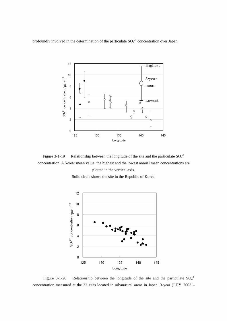
profoundly involved in the determination of the particulate SO42- concentration over Japan.

0

2

4

6

8

10

12

125 130 135 140 145

Longitude

SO

42- c

oncentr

ation /

μg・m

-3

Figure 3-1-19 Relationship between the longitude of the site and the particulate SO42-

concentration. A 5-year mean value, the highest and the lowest annual mean concentrations are

plotted in the vertical axis.

Solid circle shows the site in the Republic of Korea.

0

2

4

6

8

10

12

125 130 135 140 145

Longitude

SO

42- c

oncentr

ation /

μg・m

-3

Figure 3-1-20 Relationship between the longitude of the site and the particulate SO4

2-

concentration measured at the 32 sites located in urban/rural areas in Japan. 3-year (J.F.Y. 2003 –

Highest

Lowest

5-year mean

2005) mean concentration is plotted in the vertical axis. ② Behavior of nss-SO42- in wet deposition and particulate matters in Hedo,

Okinawa. Hedo was located as a background site on the East China Sea, and was suitable site to grasp the

effect of trans-boundary air pollution. Trans-boundary air pollution was analyzed from the observation result at the National Hedo acid deposition monitoring station and Hedo atmosphere and the aerosol observation station of National Institute of Environmental Studies.

About the daily sample collected using wet-only sampler (more than 5mm day-1) in winter (December to February) and in summer (June to August),

From the analysis result of the back trajectory method using an analysis program (NIES-CGER METEX), the nss-SO4

2- deposition vie each transportation routes which were classified into continent side and others in winter, and Southeast Asia side and the Pacific Ocean side, were calculated (Figure 3-1-21). In summer, using data totaled except for the sample influenced by the typhoon.

In winter, the nss-SO42-deposition from the continent side were increasing around from 2003 like

the northern Japan mentioned below. On the other hand, in summer, the nss-SO4

2-deposition from the Southeast Asia side was increasing, and although nss-SO4

2-concentration was low, since there was much precipitation, there was comparatively much deposition and it also had the year which is equal to the dposition in winter.

From these things, Okinawa area located in low latitude as compared with the Honshu island and near the Southeast Asia area, was suggested to be received the effect of the trans-boundary air pollution not only from China but also from Southeast Asia.

Moreover, at Hedo atmosphere and an aerosol observation station, concentration is measured for

every hour in China etc. in recent years paying attention to SO2 which the amount of discharge is increasing, and nss-SO4

2- in aerosol. Hourly trends of SO2, O3, and nss-SO4

2- from 12 to 23 March, 2005 were shown in Figure 3-1-22. The concentration of SO2 and O3 monitored by the automatic monitor at Hedo site were increasing

from the night on 17 to 18 March. In other periods, although SO2 concentrations were very low with 1 or less ppbv, these went up

about 5 ppb from 17 to 18 March. Moreover, O3 concentration went up to near the 80ppbv on March 18, although these were about

40 ppbv the previous day . Furthermore, this was interlocked with, and nss-SO4

2-(p) concentration rose rapidly and exceeded 20μg m-3.

In a weather chart, in the stage at 9:00 a.m. on March 18, a front passes through near Okinawa, it is moving to the Pacific Ocean, and the high pressure has moved to the south of Beijing after it.

At this time, the isobar is running to north and south, and it has become a situation in which an air mass tends to carry out an advection current from the direction of a continent.

0

1

2

3

4

5

nss-

SO42-

沈着

量／

mm

ol m

-2

South-East Asia

The Pacific Ocean

0

1

2

3

4

5

nss-

SO42-

Dep

osit

ion

／m

mol

m-2 The Euasian Continet

Others

Winter(Dec. - Feb.) Summer(Jun. - Aug.)

Furthermore, when the remains line of a back style is calculated using NOAAHYSPLIT4, it turns out that the advection current of the air mass has been carried out from the East Coast coastal area in China from Shanghai to the Santo peninsula in the Okinawa district after front passage.

It is 5 conjectured that SO2, O3, and the concentration rise of nss-SO42-(p) which were observed

from these things on March 18 were brought about with the air mass of the China origin. in addition to this, the same phenomenon was seen several times, and when an air mass reached

from the area along the shore from Shanghai to the Santo peninsula in China, nss-SO42-(p)

concentration was high.

Figire 3-1-22 Upper：Trends of SO2, O3, and nss-SO42- at Hedo acid deposition monitoring site and atmosphere and aerosol monitoring station Lower-berth left: the weather chart at 9:00 a.m. on 18 March Lower-berth right: result of back trajectory analysis (calculation result on the basis of 0:00, 3:00, and 6:00 a.m. on 18 March.) ③ Behavior of wet deposition of components in northern Japan In northern part of Japan, for example Hokkaido, since concentration of precipitation components is

lower than the other regions and the precipitation amount is low, wet deposition amount is not so

3/18/00 – 3/18/06

110 14013012020

30

40

Latit

ude

Longitude

3:006:00

0:00

large. It was reported that contribution of emission sources in China toward the deposition amount in

these regions is larger than the other regions and that the influence is more remarkable especially in

winter season. To examine the effect of long-range trans-boundary air pollution, we analyzed

behavior of wet deposition of components in northern Japan.

Major objects of the analysis are the dates of Rishiri and Sapporo station located on the side of Japan Sea which are subject to the effect of long-range trans-boundary air pollution. We analyzed them from year 13 downward, avoiding the influence of eruption of Miyake volcano in year 12. Figure 3-1-23 presents the annual change of precipitation amount, nss-SO4

2-, NO3- and pH. In both

stations, pH value showed a slight rising trend from year 13 to 15, but while pH value declined significantly after year 17 downward, concentrations of nss-SO4

2- and NO3- showed a increasing

trend and deposition amounts of nss-SO42-, NO3

- and H+ also increased: this is similar to the annual change of deposition amount of nss-SO4

2- in Hedomisaki in winter season. As regards to these trends of wet deposition in recent years, precipitation samples with low pH value (4.2 or less) which were able to be identified where they come form by the backward trajectory suggested a possibility of the effect of long-range trans-boundary air pollution.

④ State of long-range trans-boundary air pollution of yellow sand and O3. Since yellow sand was observed at more than 50 meteorological observatories from Tohoku to

Okinawa in 26 and 27 May year 19 and a photochemical oxidant advisory was issued in 7 prefectures

of the western Japan in 27 May year 19, we analyzed the state of the air pollution in this period.

The objects for the analysis were Tappi, Sado-seki, Ijira, Oki, Yusuhara and Ogasawara.

Figure 3-1-24 shows changes of concentrations of PM10, O3 and SO2 from 25 to 30 May.

4.0

4.5

5.0

0

5

10

15

20

25

pH

Concentr

ation / μm

ol L

-1P

recip

itat

ion A

mount

/ mm

Sapporo

4.0

4.5

5.0

0

5

10

15

20

25

pH

Concentr

ation / μm

ol L

-1P

recip

itat

ion A

mount

/ mm

Rishiri

Precipitation Amount nss-SO4 NO3 pH

The concentrations of PM10, O3 and SO2 at Oki, Yusuhara, Ijira and Sadosekimisaki changed almost

synchronously from 26 to 28 May, and the concentrations of PM10 and SO2 at Yusuhara and Ijirako

showed synchronic change with double peaks in the period. The maximum concentrations of PM10

in this period were about 300μg m-3 in the 4 regions and the maximum concentrations of O3 showed

more than 100ppb in the same period at Oki and Yusuhara as remote site. The maximum

concentration peak appeared earlier in western region in this order Oki, Yusuhara, Ijira and

Sado-seki, considering the influence of prevailing west wind in 26 to 27 May. The concentrations of

PM10 and O3 rose synchronously and the maximum concentration of PM10 was about 70μg m-3 at

Tappi in 26 May. The concentrations of PM10 and SO2 changed almost synchronously and the

maximum concentration of PM10 was over 200μg m-3 at Ogasawara from 28 to 30 May. The double

peaks of PM10 and SO2 observed at Yusuhara and Ijira was appeared after a delay of about 2 days at

Ogasawara. The concentration of O3 rose to 50 ppb and kept same level while SO2 began to be

detected and PM10 showed high concentration. Yellow sand was observed by Light Detection And

Ranging (LIDAR) at Matsue, Niigata and Sendai during the high concentration of PM10, suggesting

the increase of PM10 resulted from yellow sand. We could understand to catch the huge yellow sands

covering from Tohoku to western Japan and transported to Ogasawara keeping high concentration by

this monitoring. Increase of the concentration of O3 and SO2 linked with the observation of yellow

sand and prevailing west wind suggested the influence of long-range trans-boundary air pollution.

Figure 3-1-24 Trends of PM10、O3, and SO2 concentrations through 25 to 29 May, 2007

Figure 3-1-25 Observation results using LIDAR system at Matsue, Niigata, and Sendai through

25 to 29 May, 2007

…PM10 …O3 …SO2

0.0

0.2

0.4

0.6

0.8

1.0

0

100

200

300

5/25

5/26

5/27

5/28

5/29

5/30

Ogasawara

PM

10/μ

g m

-3 、

SO

2/pp

b

0

2

4

6

8

10

0

100

200

300

5/25

5/26

5/27

5/28

5/29

5/30

Yusuhara

PM

10/μ

g m

-3 、

SO

2/pp

b

0

2

4

6

8

0

100

200

300

5/25

5/26

5/27

5/28

5/29

5/30

Ijira

PM

10/μ

g m

-3 、

SO

2/pp

b

0

1

2

3

4

5

0

100

200

300

5/25

5/26

5/27

5/28

5/29

5/30

Oki

PM

10/μ

g m

-3 、

SO

2/pp

b

0

1

2

3

4

5

0

100

200

300

5/25

5/26

5/27

5/28

5/29

5/30

Sado-seki

PM

10/μ

g m

-3 、

SO

2/pp

b

0

1

2

3

4

5

0

20

40

60

80

100

5/25

5/26

5/27

5/28

5/29

5/30

Tappi

PM

10/μ

g m

-3 、

SO

2/pp

b

SendaiMatsue Niigata

Heig

ht

/ k

m

Heig

ht

/ k

m

Heig

ht

/ k

m

Reference 1) Kazuhide. Matsuda;Estimation of dry deposition for sulfur and nitrogen

compounds in the atmosphere - Updated parameterization of deposition velocity -,J. Jpn. Soc. Atmos. Environ. 43(6), 332-339 (2008)

2) Manabu KATAYAMA, Toshimasa OHARA, Itsushi UNO, and Hiroshi HARA, Model

Analysis of Inter-annual Variations of Sulfur Deposition in Japan; J. Jpn. Soc. Atmos.

Environ. , 43(3), 136-146 (2008) 3) Masahide Aikawa, Takatoshi Hiraki, Okihiro Oishi、Akihiro Tsuji, Hitoshi Mukai,

Kentaro Murano (2008) Acid Deposition Survey in Japan (61) - Dry deposition (Local contribution and hemispherical concentration on sulfur dioxide and particulate sulfate) - Proceedings of the 49th Annual Meeting of the Japan Society for Atmospheric Environment, p.301 (2008)

4) Nobutaka TOMOYOSE, Hisashi KADENA, Izumi NOGUCHI, Hiroshi HARA;

Temporal Trends (FY2000-2006) in Wet Deposition at Cape Hedo, Okinawa, Proceedings of the 49th Annual Meeting of the Japan Society for Atmospheric Environment, p.303 (2008).

5) Takami, A., Miyoshi, T., Shimono, A., Kaneyasu, N., Kato, S., Kajii, Y., Hatakeyama, S., :

Transport of anthropogenic aerosols from Asia and subsequent chemical transformation, J.

Geophys. Res. 112 D22S31 doi:10.1029/2006JD008120 (2007).

6) K. Hayashi, I. Noguchi, M. Aikawa, T. Ohizumi, Y. Minami, M. Kitamura, A. Takahashi, H. Tanimoto, K. Matsuda, H. Hara: Key features of wet deposition in Japan: Results of the Japanese Acid Deposition Survey for 20 years. IGACtivities Newsletter of the International Global Atmospheric Chemistry Project, 33, 2-6, 2006.

7) Yukoh IKEDA, Haruyuki HIGASHINO, Kunio IHARA, and Akira MIZOHATA, The Estimation of Acid Deposition in East Asia –Themodel development and validation-; J. Jpn. Soc. Atmos. Environ., 32(2), 116-135 (1997)

8) Masamichi INOIE, Toshimasa OHARA, Manabu KATAYAMA, and Kentaro MURANO;

Annual Source-receptor Relationships of Sulfur in East Asia Using a Numerical Simulation

Model RAMS/HYPACT, J. Aerosol Res., 20(4), 333-344 (2005)

9) Izumi NOGUCHI, Takashi YAMAGUCHI, Nobutaka TOMOYOSE, and Hiroshi HARA;

Temporal trends of wet deposition and of concentrations of dry deposition components in

Hokkaido (FY2001-2006), Proceedings of the 49th Annual Meeting of the Japan Society for Atmospheric Environment, p.304 (2008).

3.2 Results of Ecological Impact Monitoring

3.2.1 Results of Soil and Vegetation Monitoring

(1) Results of soil and vegetation monitoring from 2003 to 2007

The objectives of this survey were to obtain baseline data on soil and vegetation and to make early

detection of acid deposition impacts on forest ecosystems. Twenty-five sites (50 soil plots) of 19

areas were established in conservation areas such as national parks (NPs) or natural heritages

focusing on impacts on trees or in the areas with red-yellow soils focusing on impacts on soil. Soil

surveys and forest vegetation surveys were carried out there.

1) Acid buffering capacity of soil and effective factors to the variability

Forest soils in Japan are generally acidic. Chemical properties of soil depend on its formation

process and effective factors to the formation. Acidic soil can be produced even under natural

conditions without anthropogenic effects. Therefore, chronological changes of chemical properties

and their degrees will be evaluation criteria for assessment of impacts on soil. In this section, acid

buffering capacity of soil was evaluated taking soil types in the respective sites into consideration.

The pH (H2O) and exchangeable (Ca+Mg+K)/Al (equivalent ratio) of the surface soil of each site

were shown in Fig. 3-2-11.

Fig. 3-2-1-1 The pH (H2O) (left) and exchangeable (Ca+Mg+K)/Al (equivalent ratio) (right) of surface soil in each site

≤4.0

4.0-4.5

4.5-5.0

5.0-5.5

5.5<

Shiretoko NP●

● Towada-Hachimantai NP

Nikko NP●

Chubu-sangaku NP

●

Hodoji/ Amanosan

●

●

Daisen-Oki NPShimofuridake/ Tokusagamine Lake Bnryu

Kashiigu/ Koshosan

Kirishima-Yaku NP (2 sites)

Lake Ijira

●

●

Shikotsu-Toya NP

Bandai-Asahi NP

Hakusan NP

Ishizuchi Q-NP

●

Yoshino-Kumano NP

●●

Sekidozan/ Horyuzan

●

Aso-Kuju NP

0102030405060708090100

0123456789

10

%

Freq

uenc

y

pH (H2O)

≤0.10.1-0.50.5-1.01.0-1.51.5<

Shiretoko NP●

● Towada-Hachimantai NP

Nikko NP●

Shubu-sangaku NP

●

Hodoji/ Amanosan

●

●

Daisen-Oki NPShimofuridake/ Tokusagamine Lake Banryu

Kashiigu/ Koshosan

Kirishima-Yaku NP (2 sites)

Lake IJira

●

●

Shikotsu-Toya NP

Bandai-Asahi NP

Hakusan NP

Ishizuchi Q-NP

●

Yoshino-Kumano NP

●

Sekidozan/ Horyuzan

●

Aso-Kuju NP

0102030405060708090100

02468

101214

%

Freq

uenc

y

Ex-(Ca+Mg+K)/Al eq ratio

The soil pH (H2O) was lower than or equal to 5.0 in all the sites except for a laurel forest of

Yakushima Island or Mt. Koshosan. The pH (H2O) was lower than or equal to 4.0 especially in

Bandai-Asahi National Park (brown forest soil), Chubu-Sangaku NP (podzolic soil), Ishizuchi

Quasi-NP (brown forest soil), Houdouji Temple (red-yellow soil), and Mt. Amanosan (brown forest

soil). The pH (KCl) was lower than 4.0 in all the sites except for the laurel forest of Yakushima

Island (4.8), Mt. Koshosan (4.5), Nikko NP (4.1), and Yoshino-Kumano NP (4.1). Especially in

Ishizuchi Quasi-NP, Houdouji Temple, and Bandai-Asahi NP, significantly lower pH was recorded:

pH (H2O) was 3.8, 3.8, and 3.9, and pH (KCl) was 3.1, 3.2, and 3.4, respectively.

The equivalent ratio of exchangeable (Ca+Mg+K) to exchangeable Al (Ex-BC/Al ratio), which can

be considered as an indicator of acid buffering capacity, showed a similar tendency to pHs: the

values in the sites with significantly lower pH (< 4.0), such as Mt. Amanosan, Ishizuchi Quasi-NP,

Bandai-Asahi NP, and Houdouji Temple, were 0.06, 0.07, 0.09, and 0.09, respectively. Moreover, the

Ex-BC/Al ratio showed a relatively high positive correlation with pH (H2O) and pH (KCl) (r: 0.611

and 0.574, respectively).

Based on an acidification experiment of various

soil types, the Synthesis Report on Japan Acid

Deposition Surveys (2004) pointed out that the

Ex-BC/Al ratio can be changed by a pH 4.0 acid

precipitation in case of the soil whose Ex-BC/Al

ratio was lower than 0.1. Therefore, in the sites

with lower pH and Ex-BC/Al ratio, changes in

soil chemical properties should be monitored

continuously.

According to the Unified Soil Classification

System of Japan-2nd Approximation- (Japanese

Society of Pedology, 2002), soils in the survey

sites can be classified into four Great Groups,

namely, Brown Forest soils (14 sites), Kuroboku

soils (4 sites), Red-Yellow soils (4 sites), and

Podozolic soils (3 sites). The mean values and

standard errors of representative parameters

among each soil Great Group were shown in Fig.

3-2-1-2. In pH (H2O), Podozolic soils <

Fig. 3-2-1-2 Chemical properties of each soil Great

Groups

3.0

4.0

5.0

6.0

pH

pH(H2O)

pH(KCl)

0.0

5.0

10.0

15.0

20.0

cmol

(+) k

g-1

Ex-bases Ex-acidity

0

5

10

15 Ex-BC/Al eq ratio

Red-Yellow soils ≈ Kuroboku soils ≈ Brown Forest soils, and in pH (KCl), Podozolic soils <

Red-Yellow soils < Kuroboku soils ≈ Brown Forest soils. Exchangeable acidity was from 3 to 10

times larger than sum of exchangeable base cations (Ca, Mg, K, and Na) in all the soil Great Groups,

reflecting low pH of the soils. Especially in Podozolic soils and Red-Yellow soils, the difference

between the sum of base cations and the acidity was significantly larger, suggesting less base cations

and more acidity.

In Ex-BC/Al ratio, Podozolic soils (0.1) < Red-Yellow soils (0.3) ≈ Kuroboku soils (0.5) << Brown

Forest soils (7.6). The larger mean value of Brown Forest soils can be attributed to a base-rich soil in

the laurel forest of Yakushima Island. When this significantly larger value is removed, the mean

value will be 1.2. Variation among Brown Forest soils was quite large. As mentioned above, the

survey sites showing relatively high acidity, represented by Ishizuchi Quasi-NP, Bandai-Asahi NP,

Mt. Amanosan, could also be found.

Soil monitoring was carried out taking effective factors to variability of the obtained data into

account. As the effective factors in the field sampling, several sampling levels, such as “area”, “soil

type (site)”, “plot”, and “subplot”, were considered. Cumulative contributions of these sampling

levels to the data variability were shown in Fig. 3-2-1-3.

Fig. 3-2-1-3 Soil sampling system (left) and cumulative contributions to variance in chemical properties of

surface soils (right). The data in Mt. Koshosan, which showed significantly larger variations among plots and

subplots, were not included in the analysis.

Area 18

Soil type 1 or 2Plot 2Subplot 5Repeat analysis 2 times

0102030405060708090

100

Cumulative contribution,

%

pH(H2O) Ex-Ca Ex-Al

In soil pH and Ex-Al, indicators of acidity, “soil types” had much effect on the total variability,

reflecting difference of soil acidity in the respective soil types. In Ex-Ca, “subplots” and “area” had

much effect on the total variability; the former one might reflect spatial heterogeneity of soil, such as

thickness of organic layer, and the latter one might reflect geology or climate than soil type.

2) Evaluation of soil acidification trends

Most survey sites focusing on soil acidification were established in 2001 and Red-Yellow soils or

similar types of soil were selected with their reference types of soil in each area. According to the

Long-Term Monitoring Program, the second surveys were carried out for all the sites until 2007,

while the sampling intervals were varied from 2 to 6 years. The mean values among the respective

plots (mean of five subplots) in these sites were shown in Table 3-2-1-1.

Note. Superscripts, * and **, indicate significant difference at 5% level and 1% level, respectively, by the t-test for the mean

values of subplots.

Table 3-2-1-1　Changes of chemical properties of surface soils (0-10 cm) in Red-Yellow soilsECEC BS

H2O KCｌ %Ishikawa Pref. Sekidozan Brown forest soils 1 2001 4.4 3.7 15.29 8.02 0.08

2005 4.3 3.5** 14.82 10.83 0.122 2001 4.5 3.8 13.16 11.19 0.13

2005 4.4 3.5** 13.50 12.38 0.15Horyuzan Red soils 1 2001 4.6 3.8 17.17 9.87 0.10

2005 4.6 3.6 17.20 8.50 0.092 2001 4.6 3.8 19.67 12.38 0.13

2005 4.6 3.6** 19.18 10.51 0.11Osaka Pref. Amanosan Reddish brown forest soils 1 2001 4.2 3.4 9.16 9.07 0.11

2007 4.1 3.4 9.03 5.22* 0.06*2 2001 3.8 3.1 11.10 6.55 0.08

2007 4.0 3.3 10.47 4.72 0.05Hodoji Yellow soils 1 2001 3.9 3.2 11.29 5.24 0.06

2007 3.8 3.1 10.51 9.12* 0.10*2 2001 4.0 3.3 8.31 7.40 0.09

2007 3.9 3.2 9.13 8.14 0.09Shimane Pref. Lake Banryu Brown forest soils 1 2001 4.8 3.9 4.30 17.07 0.21

2006 4.9 3.8 5.13 30.39* 0.532 2001 4.7 3.7 4.86 27.10 0.44

2006 4.8 3.9* 4.83 21.97 0.33Iwami-rinku FP Red soils 1 2001 4.3 3.5 8.56 16.51 0.22

2006 4.5 3.7 7.58 15.65 0.212 2001 4.2 3.3 10.61 10.72 0.12

2006 4.4 3.6 10.53 12.60 0.16Yamaguchi Pref. Tokusagamine Kuroboku soils 1 2001 4.6 3.8 11.87 10.08 0.12

2003 4.5 3.9* 11.43 13.03 0.202 2001 4.6 3.8 12.22 13.09 0.20

2003 4.6 3.9 11.39 10.01 0.13Simofuridake Yellow soils 1 2001 4.9 3.9 5.18 31.14 0.77

2003 4.9 3.9 4.87 36.01 0.842 2001 4.8 3.9 4.45 25.95 0.47

2003 5.0 4.0 4.05 36.11 0.97Fukuoka Pref. Kashiigu Reddish brown forest soils 1 2001 4.2 3.4 19.00 13.04 0.17

2007 4.1 3.3 18.71 8.57 0.092 2001 4.5 3.5 27.90 25.03 0.42

2007 4.4 3.4 23.62 15.13 0.18Koshosan Brown forest soils 1 2001 4.8 3.9 14.23 51.29 >1.0

2007 4.5 3.6 8.35 40.22 0.842 2001 6.5 5.6 30.54 90.49 >1.5

2007 6.1 5.4 25.50 78.40 >1.5

Ex-(Ca+Mg+K)/Al eq ratiocmol(+) kg-1Area Site Soil type Plot Survey

year

pH

Most plots showed no clear acidification trend but two sites in Ishikawa Pref. showed significant

decrease of pH (KCl). Soil acidity in these sites may increase, since pH (KCl) indicates potential

acidity of soil. In Plot 1 of Mt. Amanosan (Osaka Pref.), pH (H2O) and pH (KCl) showed mostly

same levels but base saturation and Ex-BC/Al ratio showed significant decrease. In these sites,

Ex-BC/Al ratio was low, approx. 0.1, and therefore, the soils may be sensitive to acid deposition, as

mentioned above. The continuous surveys are necessary in these sites. On the other hand, the

opposite tendency, increase of parameters, was also found; base saturation and pH (KCl) at Lake

Banryu (Shimane Pref.), pH (KCl) at Mt. Tokusagamine (Yamaguchi Pref.), and base saturation and

Ex-BC/Al ratio at Houdouji Temple (Osaka Pref.). Especially around Lake Banryu, changes in

conditions of the catchment area may be related to the data, since forest managements for pine

wilting decease have been carried out for the last decade.

The changes in pH (H2O) and Ex-Al of the surface soil horizon (3 - 5 cm depths) and the subsequent

soil horizon (10 – 15 cm depths) were shown for the long-term monitoring plots in the Lake Ijira

Catchment site. The pH (H2O) decreased continuously in the surface horizon and subsequent horizon

at all five plots for 14 year from 1990 to 2004, while some fluctuations could be found. The mean

pH (H2O) of the surface layer (collected by the fixed depth, 0 - 10 cm) among two plots for the

EANET monitoring were 4.3 (3.9 - 4.4) in 2006, and it can be clarified that these plots were also

acidified similarly to the long-term plots. The Ex-Al, an indicator of acidity, showed increasing

trends in most plots especially for the surface horizon, and in a few plots for the subsequent horizon.

In the Lake Ijira catchment, as described in the section 3.3, a wet deposition amount of H+ is the

highest level in Japan, and the river water chemistry showed several acidification phenomena, such

as, temporary SO42- leaching, decrease of the water pH, and continuous increase of the NO3

-

concentration. Therefore, changes in the soil chemical properties can be considered as a part of the

acidification process in the whole catchment area.

Since soil pH may decrease due to a rapid uptake of nutrient bases during plant growth periods, it

may be necessary to evaluate the respective contributions of H+ production in the ecosystem and H+

input from the atmosphere to the soil acidification in detail. However, as shown in the section 3.3,

the tree growth rates in the Lake Ijira catchment showed decreasing trends during the sampling

period of soil. The rapid decrease of soil pH observed here cannot be explained only by plant uptake.

In the catchment, since forest managements such as thinning had not been carried out, the

management conditions should also be considered. However, taking the highest level of wet

deposition amounts in Japan, the high acid loading seems to be a main cause of soil acidification.

The soil pH (H2O) decreased to the significantly lower level, 3.9 in average in the surface soil. In the

buffering process of soil, buffering reactions by Al-(hydro)-oxide may occur mainly in the pH range,

and Al3+ toxic to plant growth can be leached into the soil water. Therefore, it may be necessary to

monitor effects of the soil acidification on plant physiology in future.

3) Assessment of tree decline conditions

Figure 3-2-1-5 showed the mean values of “Dieback of stem” and “Density of foliage”, which were

observed as indicess of tree decline symptoms. The indices were recorded according to 5- or 4-class

decline scales, from 0 (healthy) to 5 (dead) in case of “Dieback of stem” or 4 (dead) in case of

“Density of foliage”. The larger values showed clearer decline symptoms.

Some decline symptoms were observed in 17 sites among 25 sites, while small changes of tree forms

in Mt. Sekidozan and Mt. Amanosan were not included in the figure. The cumulative values of two

parameters were the largest in Chubu-Sangaku NP and then in Yoshino-Kumano NP, where more

than half of trees showed some symptoms. In Yoshino-Kumano NP, typhoons may be a main cause

of the symptoms, which were observed in Fagus crenata and Abies homolepis. In Chubu-sangaku

Fig. 3-2-1-4 Chronological changes in pH (H2O) and exchangeable Al of soils at long-term monitoring

plots in the Lake Ijira Catchment site

Surface layer, until 3 – 5 cm depths; subsequent layer, until 10 – 15 cm depths. The measurement of pH(H2O)

was done by the following soil:solution ratio: 1:5 until 1992, and 1:2.5 from 1993.

2

4

6

8

10

12

14

16

cmol

(+) k

g-1

Plot 37Plot 38Plot 41Plot 46Plot 49

c)Surface soil Ex-Al

2

4

6

8

10

12

14

16Plot 37Plot 38Plot 41Plot 46Plot 49

d)Subsoil Ex-Al

3.6

3.8

4

4.2

4.4

4.6

4.8

5

5.2

5.4

pH(H

2O)

Plot 37Plot 38Plot 41Plot 46Plot 49

a)Suface soil pH(H2O)

3.6

3.8

4

4.2

4.4

4.6

4.8

5

5.2

5.4Plot 37Plot 38Plot 41Plot 46Plot 49

b)Subsoil pH(H2O)

NP, the cause has not been identified but small precipitation amounts during the growing period in

2007 were pointed out. In other sites also, the declining trees, which were mainly caused by acid

deposition or soil acidification, were not identified.

Chronological changes in “Vitality of trees” recorded as the total index of tree decline were shown in

Fig. 3-2-1-6. The tree decline symptoms that were processed from 2004 to 2005 seemed to be

recovered in the later years in Shikotsu-Toya NP, Nikko NP, Daisen-Oki NP, and Ishizuchi Quasi-NP.

It was suggested that damages by typhoons in 2003 were recovered after a few years. It is difficult

by the observation to clearly distinguish changes by acid deposition or air pollution from changes by

meteorological events/conditions, such as typhoons, cold summer, and draught stress, especially in

the previous surveys until 2002, because the observation was done only once 3 – 5 years. However,

the observation has been done at least once a year since 2003 according to the Long-Term

Monitoring Plan, and therefore, it may be possible to distinguish effects of meteorological

events/conditions. In the Lake Ijira catchment, a thinning of the dense forest as a forest management

was done just after the observation of 2006, and the recovery has already been observed in 2007.

Figure 3-2-1-5 Major tree species and conditions on “Dieback of stem” and “Density of foliage” in 2007.

The column graph shows cumulative values of the means of two parameters in the respective plots (the larger values

shows clearer decline symptoms).

0.00 0.20 0.40 0.60 0.80 1.00 1.20 1.40 1.60

Shiretoko NPShikotsu-Toya NP

Towada-Hachimantai NPBandai-Asahi NP

Nikko NPChubu-sangaku NP

Hakusan NPYoshino-Kumano NP

Daisen-Oki NPIshizuchi Q-NP

Aso-Kuju NPYaku-1Yaku-2

SekidozanHoryuzan

HodojiAmanosan

ShimofuridakeTokusagamine

KashiiguKoshosanLake Ijira

YamatoLake Banryu

Iwami-rinku FP

Dieback of stem

Density of foliage

Major tree speciesFir/ BirchBirch/ MapleFir BeechBeech/ FirBeech/ MagnoliaBeechBeech/ FirBeechBeech/Clethra/ BirchOak/ BeechJapanese cedarSakaki/ CamelliaBeechBeechJapanese chinquapinJapanese cypressEurya japonica/ OakJapanese cypressJapanese chinquapin/BayberryEvergreen oak/ JapanesechinquapinJapanse cypressJapanse cypressPerseaJapanese chinquapin/ Persea

On the other hand, it seemed that the tree decline symptoms were gradually processed in Shiretoko

NP, Chubu-Sangaku NP, Yoshino-Kumano NP, Hakusan NP, and Houdouji Temple. In these sites,

suppression by other surrounding trees or damages by strong winds were suggested as possible main

causes. However, the soil pH (H2O) was significantly low in Houdouji Temple as described above. It

can be suggested that continuous observations should be done carefully in these sites.

As a part of forest vegetation monitoring, description of trees (measurement of tree size or growth)

and surveys on species composition in understory vegetation have also been done and the data has

been accumulated. At the present, the first surveys have just finished in the last five years, and it is

be expected that growth rates of trees in the respective sites will be evaluated in future.

(2) Quality assurance/quality control (QA/QC) of the data

The data quality is assured through the audit of the national center of Japan, ADORC, and in this

occasion, design of the monitoring plots and sampling procedures in the sites and conditions of the

laboratories are confirmed. As for analytical precisions of soil, variations in the repeatability

Fig. 3-2-1-6 Chronological changes in “Vitality of trees” (the larger value shows severer decline.)

0.00

0.10

0.20

0.30

0.40

0.50

0.60

0.70

0.80

0.90

1.00Shiretoko NP

Shikotsu-Toya NP

Towada-Hachimantai NPNikko NP

Chubu-sangaku NP

Hakusan NP

Yoshino-Kumano NP

Daisen-Oki NP

Ishizuchi Quasi-NP

0.00

0.10

0.20

0.30

0.40

0.50

0.60

0.70

0.80

0.90

1.00

15 16 17 18 19

Vita

lity

of tr

ees

Horyuzan

Hodoji

Shimofuridake

15 16 17 18 19

Kashiigu

Koshosan

Lake Ijira

Yamato

Lake Banryu

Iwami-rinku FP

condition, within-laboratory reproducibility condition, and reproducibility condition were

significantly small and their precisions might be enough high according to the results of the

inter-laboratory comparison projects on soil. The reliable data may be obtained in the surveys.

3.2.2. Results of Monitoring on Inland Aquatic Environment

(1) Results of monitoring on inland aquatic environment from 2003 to 2007

In this survey, 11 lakes and their inflow/outflow rivers with low EC and low alkalinity, which may

be susceptible to acidification, were selected as the monitoring sites. The mean values of the

representative parameters from 2003 to 2007 in the respective monitoring sites were shown in Table

3-2-2-1. The alkalinity in most sites was lower than 0.200 mmolc L-1. Lake Futagoike (Oike), Lake

Yashagaike, and Lake Sawanoike may be the most sensitive to acid deposition, showing the lowest

level of alkalinity and pH; lower than 0.030 mmolc L-1 and lower than pH 5.8, respectively. In all the

lakes including these sensitive ones, obvious effects of acid deposition were not identified. On the

other hand, alkalinity and pH in Lake Nagatomiike were significantly higher than other lakes. Lake

Sankyoike and Lake Banryu had large effects of sea salts and the water was dominated by Cl- and

Na+. The NO3- concentration was the highest in the surface water of Lake Ijira and inflow rivers

among the monitoring sites. The features of the catchment areas were shown in Table 3-2-2-1 (b).

Table 3-2-2-1(a) Mean values of representative parameters in the monitoring lakes from 2003 to 2007

*1:Less than detection limit

Location Lake or River name Point pH EC Alkalinity SO42- NO3

- Cl- NH4+ Na+ K+ Ca2+ Mg2+

Prefecture mS m-1 mmolc L-1 μmolc L-1

Yamagata. Imagamioike Surface 6.37 3.90 0.071 80.7 *1 175.3 *1 226.1 11.1 26.0 43.3

Tochigi Karikomiko Surface 6.91 3.25 0.156 115.2 5.3 20.0 1.4 131.0 14.0 117.8 14.3

Nagano Futafoike(Oike) Surface 7.02 1.86 0.112 33.4 15.9 11.3 0.7 46.1 6.4 107.4 15.8

Futagoike(Meike) Surface 5.73 0.73 0.020 29.3 4.1 10.0 0.7 13.7 4.1 22.1 7.5

Niigata Sankyoike Surface 6.87 8.49 0.109 92.8 2.1 542.6 1.1 510.9 30.9 81.8 113.8

Ishikawa Ohataike Surface 6.53 4.29 0.134 33.5 8.6 186.5 2.5 197.1 25.8 65.0 70.1

Fukui Yashagaike Surface 5.36 1.64 0.017 42.7 7.5 61.3 4.9 59.7 8.5 20.3 18.2

Gifu Ijira Surface 7.03 4.24 0.163 108.8 31.0 64.7 3.5 91.9 7.9 153.3 110.7

Kamgatani river Inflow 6.96 4.43 0.140 136.2 39.6 63.2 *1 93.8 7.3 150.4 122.8

Kobora river Inflow 6.72 3.86 0.125 101.6 33.3 68.9 *1 102.5 6.5 100.5 116.5

Kyoto Sawanoike Surface 5.70 1.73 0.021 32.2 *1 83.4 *1 65.7 6.4 30.1 30.6

Shimane Banryu Surface 7.06 10.65 0.166 88.1 1.7 634.3 1.8 605.5 47.6 66.1 141.0

Banryu No.3 Surface 7.05 10.60 0.173 89.9 2.1 624.5 1.4 604.4 47.9 72.2 142.5

Yamaguchi Yamanokuchi dam Surface 6.64 6.02 0.107 97.8 9.7 285.8 *1 332.4 25.1 65.6 72.2

Kagawa Nagatomike Surface 7.34 9.53 0.512 169.5 25.4 155.2 5.2 339.3 25.4 416.4 104.8

-0.8

-0.6

-0.4

-0.2

0

0.2

0.4

0.6

0.8

1

1.2

-0.6 -0.4 -0.2 0 0.2 0.4 0.6 0.8 1 1.2

SO42-

H+

NH4+

Ca2+

Alkalinity

EC

Na+K+

Cl-

NO3-

Mg2+

-2

-1.5

-1

-0.5

0

0.5

1

1.5

2

-1.5 -1 -0.5 0 0.5 1 1.5 2 2.5

Kamagatani river

Kobora river

Lake Ijira

Lake Karikomi

Lake Futago (Oike)

Futagoike (Meike)

YashagaikeSawanoike

Imagamioike

Lake Banryu

Lake Banryu No.3Yamanokuchi dam

SankyoikeOhataike

Table 3-2-2-1(b) Features of the respective catchment areas

Location Lake name Surface stratum Soil type Vegetation

Yamagata Imagamioike Partially consolidated Drained podsol Fagus crenata, Sasa kurilensis

Tochigi Karikomiko Rhyolite, Andesite Aquic and Drained podsol Abies mariesii, Abies veitchii

Nagano Futafoike Lava Aquic humic podsol Smilacina viridiflora, Betula ermanii

Niigata Sankyoike Neogene period sediment Brown forest soil Quercus crispula, Quercus serrata

Ishikawa Ohataike Rhyolite, Andesite Drained brown forest soil Castanea, Quercus crispula

Fukui Yashagaike Sandstone, Shale, Chert Brown forest soil Fagus crenata, Lindera umbellata var. membranacea

Gifu Ijirako Chert Brown forest soil Pinus densiflora､Chamaecyparis obtusa

Kyoto Sawanoike Chert Drained brown forest soil Pinus densiflora, Quercus serrata

Shimane Banryuko Quaternary period sediment Residual regosol Pinus densiflora, Pinus thunbergii

Yamaguchi Yamanokuchi dam Rhyolite Brown forest soil Rhododendron reticulatum、Pinus densiflora

Kagawa Nagatomike Diorite Drained brown forest soil Quercus acutissima, Quercus serrata,

The principal component analysis (PCA) was applied to the mean values of the monitoring sites, and

loadings of two major factors (a) and principal component scores (b) were shown in Fig. 3-2-2-1.

The first factor loading (X axis) was 45.0% and the second factor loading (Y axis) was 33.9%, and

more than 75% was explained by two axes. The data of Lake Nagatomiike with significant high

alkalinity and Ca2+ was omitted in this analysis. The PCA was applied only to the acid sensitive

lakes with low alkalinity (< 0.200mmolc L-1), and therefore, characteristics of the respective

lakes/catchments were confirmed in detail. Fig. 3-2-2-1 Factor loadings (a) in the principal component analysis and principal component

scores (b) of the respective monitoring lakes

As for the loadings of two major factors (see Fig. 3-2-2-1 a), the first factor loadings (X axis) of EC

(b) (a)

and many ions such as sea-salt-origin ions, Mg2+ and K+ showed positive high values, indicating

amounts of dissolved ions in the water. The second factor loadings (Y axis) of Ca2+ and alkalinity

showed high positive values, while the loading of H+ showed negative value, indicating acidity of

the water. Moreover, the loadings of SO42- and NO3

- showed positive high values, suggesting

effects of these ions.

As for the scores of each monitoring site (see Fig. 3-2-2-1 b), Lake Sankyoike and Lake Banryu

showed high values on X axis because of their high EC, Na+, and Cl- suggesting effects of sea salts.

The third quadrant may show the category of acid-sensitive lakes, whose acidity is high and ion

concentration is low. The waters at Lake Yashagaike, Lake Futagoike (Meike), and Lake Sawanoike,

which were located in the third quadrant, were high acid sensitive and therefore, acidification of

these lakes should be carefully monitored. Lake Imagamioike was also located in the third quadrant

and might be relatively acid sensitive. On the other hand, Lake Ijira, which has been acidified, was

located in the second quadrant, showing less acidity compared with the lakes such as Lake

Yashagaike. However, concentrations of SO42- and NO3

- at Lake Ijira were very high, suggesting

effects of NO3- leaching by N saturation and high SO4

2- leaching, as discussed later in the section 3.3.

Lake Ijira should also be carefully monitored, since the acidification status may be different from

those at the third quadrant. Lake Karikomi may have effects of high concentrations of SO42- and

Ca2+. (2) Long-term acidification trends of inland waters A long-term trend analysis was done for major parameters by using the seasonal Mann-Kendall tests (Hirsch et al, 1982) as shown in Table 3-2-2-2. The analysis was applied only for several long-term monitoring sites. Table 3-2-2-2 Long-term trend analysis of major parameters in the surface water or inflow rivers of the monitoring lakes

Notice: Asterisks, *, **, and ***, shows significant levels, P < 0.05, 0.01, and 0.001, respectively, by long-term trend analysis of seasonal Mann-Kendall tests using 3 or 4 times yearly seasonal data.

Lake or River name Duration N Z-score

pH EC Alkalinity SO42- NO3

- Cl- NH4+ Na+ K+ Ca2+ Mg2+

Hutagoike(Oike) 1998-2007 30 1.56 1.83 1.35 4.94*** 0.52 -0.31 -0.29 2.35** -1.74 2.18* 1.26

Hutagoike(Meike) 1998-2007 30 -0.98 -1.77 0.73 3.53*** -1.66 -0.73 -1.83 2.94** -1.84 0.05 -0.64

Sankyoike 2001-2007 27 -1.52 0.95 0.96 0.00 0.24 0.87 -0.78 0.16 -0.48 0.39 0.00

Yasyagaike 2000-2007 41 -1.81 -1.10 -2.27* -1.23 1.55 -2.58** -0.66 -2.00* 0.97 -1.17 -0.91

Ijirako 1988-2007 76 -0.74 5.68*** 5.45*** 0.87 5.43*** 2.3* 1.89 0.89 -0.56 3.60*** 2.55*

Kamagatani river 1988-2007 77 -2.07* 3.28** 1.19 1.03 6.00*** 2.49* -0.11 0.96 -0.05 1.49 1.68

Kobara river 1988-2007 57 -1.00 5.43*** 1.66 2.20* 5.36*** 2.28* -0.41 2.87** 1.82 2.20* 3.16**

Banryuko 1989-2007 76 2.49* 5.14*** 5.63*** -0.47 0.84 4.96*** -1.98* 6.00*** 1.16 -0.97 3.61***

Banryuko No3. 1989-2007 76 2.40* 5.71*** 4.60*** 0.00 -0.11 4.28*** -1.61 5.61*** 0.83 0.13 3.11**

Kamagatani River (an inflow river to Lake Ijira) showed a significant declining trend of pH (p <

0.05). As suggested in the Synthesis Report on Japan Acid Deposition Surveys (2004), a remarkable

pH decline was seen since 1996 at Kamagatani river, but the trend became mostly flat since 2004

(Fig. 3-2-2-2 (a)). On the other hand, a significant increasing trend of pH was found in Lake Banryu

(Fig. 3-2-2-2 (d)). A significant declining trend of alkalinity was seen in Lake Yashagaike, while the

increasing trend was seen in Lake Ijira and Lake Banryu (Fig. 3-2-2-2 (e)).

Ca2+

(µm

olc L

-1)

6.00

6.50

7.00

7.50

8.00

8.50

1988/1/1 1994/1/1 2000/1/1 2006/1/1

pH

0

100

200

300

400

500

1988/1/1 1994/1/1 2000/1/1 2006/1/1

Ca2

+(μm

olc/L

)

Fig. 3-2-2-2(c) Fig. 3-2-2-2(d)

Ca2+changes at Lake Ijira pH changes at Lake Banryu

The peak as 1997 is unknown

Fif. 3-2-2-2(a) Fig. 3-2-2-2(b)

pH changes at Kamagatani river NO3- changes at Kamagatani river

0

20

40

60

80

100

1988/1/1 1994/1/1 2000/1/1 2006/1/1

NO

3-（μm

olc/L

）

6.00

6.50

7.00

7.50

8.00

8.50

1985/1/1 1991/1/1 1997/1/1 2003/1/1

pH

NO

3- (µm

olc L

-1)

400

450

500

550

600

650

700

1988/1/1 1994/1/1 2000/1/1 2006/1/1

Cl-(μm

olc/L

）

Fig. 3-2-2-2(e) Fig. 3-2-2-2(f)

Alkalinity changes at Lake Banryu Cl- changes at Lake Banryu

0.000

0.050

0.100

0.150

0.200

0.250

1988/1/1 1994/1/1 2000/1/1 2006/1/1

Alk

alin

ity(m

mol

c/L）

Cl- (µ

mol

c L-1

)

Alk

alin

ity (m

mol

c L-1

)

Fig. 3-2-2-3 Changes of number of flagged data in the inter-laboratory comparison projects for the last five years.

0%

10%

20%

30%

40%

50%

60%

70%

80%

90%

100%

2003 2004 2005 2006 2007

95.0 92.6 95.9 93.4

97.5

E:5.0 E:6.6 E:4.1 E:6.6 E:2.5 X:0.0 X:0.8 X:0.0 X:0.0 X:0.0

X E Data within DQOs

At the Lake Ijira catchment, a significant increasing trend of NO3- concentration was seen in the

surface water of the lake and two inflow rivers (Fig. 3-2-2-2 (b)). As mentioned above, the pH of

Kamagatani River showed the declining trend, while the alkalinity of the lake surface water showed

the increasing trend. Moreover, concentrations of base cations such as Ca2+ and Mg2+ also showed

increasing trends in the lake surface water and Kobora River, another inflow river (Fig. 3-2-2-2 (c)).

Significant increasing trends of SO42- concentration was seen in Lakes Futagoike (twin lakes, Oike

and Meike). At the Lake Oike, concentrations of Na+ and Ca2+ showed a significant increasing trend.

At the Lake Banryu, where the alkalinity shows the increasing trend, Na+, Cl-, Mg2+ showed the

increasing trend (Fig. 3-2-2-2 (f)). Sea-salt-origin ions or ions derived from anthropogenic activities

seemed to be increasing there, while Ca2+ concentration showed no clear trend.Concentrations of

Na+ and Cl- showed a significant declining trend at the Lake Yashagaike, which was classified into

the most acid-sensitive lakes (see Fig. 3-2-2-1).

(2) Quality assurance/quality control (QA/QC) of the data

The data quality is assured through the audit of

the national center of Japan, ADORC, and in this

occasion, sampling procedures at the sites and

conditions of the laboratories are confirmed. Results

of the inter-laboratory comparison projects for the

last five years were shown in Fig. 3-2-2-3. Through

all the projects, the data more than 90% satisfied the

data quality objectives. The laboratories seemed to

keep relatively high data quality for the period. It

was clarified that cations (low concentration or

divalent ions) showed flagged data more frequently

than pH, EC, and anions and larger variations among

the laboratories. Efforts should be made for the data

quality of cations.

3.2.3 Discussion on ecological effects of acid deposition

As described above, during the last five years, obvious acidification trends and related tree decline

phenomena were not reported in most sites, while soil acidification was found in the Lake Ijira

catchment. Since a few plots’ pHs were lower than 4.0 in the Lake Ijira catchment, the soil

acidification and its effects on trees should be monitored and carefully evaluated. As described later

in the section 3.3, acidification phenomena have been reported recently in the Lake Ijira catchment,

suggesting effects of acid deposition. In some areas whose soil or geology may have low acid

buffering capacity, a long-term acidification trend of rivers was reported. In this sub-section,

referring the previous research facts, hot spots, the area with high risk of acidification, were

identified based on soil or geological features and acid deposition amounts.

(1) Identification of acid-sensitive areas

As for spatial distribution of sensitivities to acid deposition, Environment Agency of Japan and

Japanese Society of Soil Science and Plant Nutrition have compiled “the Map for assessing

susceptibility of Japanese soils to acid precipitation (1:2,000,000)” in 1983 (Fig. 3-2-3-1). In the map,

Japanese major soil types were classified into 6 classes and a distribution of each class was shown

on a soil map of Japan (the classification was updated and merged into 3 classes in 1994). According

to the map, soils with low acid buffering capacity, such as regosols (immature soils), red-yellow soils,

and brown forest soils (dry type), are distributed mainly in Southeast Japan. The map was created

based on acid buffering capacity of soils. However, chemical components of rocks or minerals as a

parent material of soil, their weathering rate, and tolerance of ecosystems (vegetation) may be

related to the sensitivity of each area.

Taking the questions above into account, Yoshinaga et al. (1994) created a map of relative sensitivity

to acid deposition for Japan Islands by using Digital National Land Information according to the

method of Stockholm Environment Institute (SEI method). In the SEI method, four parameters,

including geology, soil, land-use, and precipitation are taken into account and 5-class evaluation

(from 1 to 5) are applied to each parameter. As a result, the areas with the following conditions

become the most sensitive; whose precipitation amount is more than 1200 mm, dominated by

coniferous species, and covered by soils derived from silicate-rich rocks with low weathering rate.

The most sensitive points with the highest score, 5, can be found mostly in the area, where granite

rocks are distributed, mostly in Southeast Japan. The sensitive points showing the score, 4, were

distributed also in granite-rock areas or coniferous forests in Hokkaido. These high-sensitive areas

included the areas covered by granite rocks in Kii Peninsula, Chubu (Central) Mountains including

Gifu Prefecture, and Asahi Mountains in the north part of Niigata Prefecture, in addition to Southeast

Japan. In the SEI method, the precipitation amount, 1200 mm, was used as a threshold but most part

of Japan may have larger precipitation. Therefore, difference cannot be clarified by the precipitation,

and this may be one of problems on applicability of this method to Japan.

Based on the previous approaches above, as acid-sensitive ecosystems, the areas, where silicate-rich

rocks such as granite are distributed, and also which were mainly covered by acid-sensitive soils,

such as immature soils, red-yellow soils, and brown forest soils (dry type), can be identified.

Fig. 3-2-3-1 Map for assessing susceptibility of Japanese soils to acid precipitation (Environment Agency

of Japan and Japanese Society of Soil Science and Plant Nutrition, 1983)

Highly tolerant Gley soils, Dark Red soils (derived from basic

rocks), and Dark Red soils in Okinawa

Gray/Brown Lowland soils, Andosols, other

Dark Red soils

Moderately tolerant Light-colored Andosols, Brown Forest soils

Dry-type Brown Forest soils, Andosols

(nonallophanic), Podzols, Peat soils

Poorly tolerant Pyroclastic Regosols and Lithosols, Poorly

buffered Peat soils, Red-Yellow

Podzolic/Lithosolic soils

Sand-dune soils, Lithosols, Alpine Lithosols

Although the map by Yoshinaga et al. does not include Yakushima Island in South Kyushu, the

island is famous for granite. Vegetation types should also be considered but most part of Japanese

forest is covered by planted coniferous species, such as Cryptomeria japonica or Chamaecyparis

obtusa. Further investigation is necessary on evaluation of vegetation distribution.

(2) Distribution of wet deposition

Effects of acid deposition on ecosystems

may become obvious in the areas, which are

highly acid-sensitive and also whose

deposition is significantly large. Since it

takes a long time for changes in soil

chemical properties, deposition amounts in

the past such as 1960s’ or cumulative

amounts should also be considered. At

present, deposition amounts in the past were

not available enough but surrounding areas

of mega cities or industrial areas should be

taken into consideration.

Distribution of the monitoring sites with

high wet H+ deposition was shown in Fig.

3-2-3-2. The map was created based on the

surveys by Japan Environment Laboratories

Association (JELA) (1999 – 2004) and

MOEJ (1998 – 2004) for evaluation of regional watershed acidification, which was discussed in the

section 3.3. Although contribution of dry deposition should also be considered, a spatial distribution

of wet deposition was discussed tentatively in this evaluation because of its high data availability.

The sites with high wet H+ deposition were distributed in Chubu region including Lake Ijira,

Shizuoka, and the coastal area along the Sea of Japan, Shikoku Island, South Kyushu, and

Yakushima Island. As described in the section 3.3, the deposition characteristics are different among

these sites. In the south part of Japan, such as Shikoku Island, South Kyushu, and Yakushima Island,

the concentration was relatively low but the precipitation amount was significantly high, and

therefore, the deposition amount was the highest levels in Japan. On the other hand, in Chubu region,

including Lake Ijira and the coastal area along the Sea of Japan, both concentration and precipitation

were relatively high, and therefore, the deposition amount was the highest levels in Japan. These

deposition characteristics should also be considered for the evaluation in future.

Fig. 3-2-3-2 Distribution of the monitoring sites with high wet H+

deposition in Japan The wet deposition of H+ at the red colored

sites is within 10% highest among 120 sites.

(3) Hot spots to be monitored

As highly acid-sensitive ecosystems, the forest areas, where silicate-rich acid rocks such as granite

are distributed and which is covered by immature soils, red-yellow soils, or brown forest soils (dry

type), can be considered and these areas may be distributed in the north part of Niigata Prefecture,

Chubu region, Kii Peninsula, and Southeast Japan. Taking the wet deposition amount into account,

south part of Chubu region including Lake Ijira, the coastal area of Chubu region along the Sea of

Japan including Niigata Prefecture, South Kyushu, and Yakushima Island can be identified as hot

spots. As discussed later in the section 3.3, the long-term declining trend of the river water pH was

reported in Gifu Prefecture and the north part of Niigata Prefecture. Especially in Niigata Prefecture,

the relationship with geology was obvious. In these areas, acidification on the watershed scale,

including soil and river, should be considered. Possibility of long-term soil acidification should be

checked in the areas and an investigation of the soil plots surveyed in the past can be one of the

options. In case of Yakushima Island, the soil layer is relatively thin, and also the direct runoff may

have large contribution to water discharge taking steep geographical conditions of the island into

account. It may be possible that much water not enough neutralized in the soil layer is flowed into

streams/rivers in such a condition. Effects on streams/rivers and aquatic organisms should mainly be

considered there.

In addition to the hot spots identified above, North Kyushu and Seto Island Sea region should also

carefully evaluated, although these regions were not identified as high-deposition areas. Because

major industrial areas are located in these regions and it seemed emission from these areas were

significantly much in the past.

Discussion above mainly focused on the watershed/catchment scale acidification including soil and

river. However, direct effects of acidic/oxidizing pollutants on trees should also be considered for

identification of hot spots. Taking recent increasing trends of ozone concentrations and widespread

Photochemical Oxidants Warning into account, direct exposure effects of ozone on plants should be

evaluated. Calculation of AOT40 using the available ozone data and measurement of ozone

concentrations in forest area by using passive samplers should be considered. Through the activities,

the areas, where the ozone concentration is higher than certain threshold, should be identified, and

then, the monitoring system focusing on ozone effects, such as observation of specific visible injury,

should be developed in future.

References

1) Yoshinaga et al. (1994) Mapping of relative sensitivity to acid deposition for Japan Islands by

utilizing Digital National Land Information. Japanese Journal of Soil Science and Plant

Nutrition, 65, 565-568.

2) Hettelingh et al., 1991. Mapping critical loads for Europe, CCE Technical Report, No.1, p.86,

Coodinate Center for Effects, National Institute of Public Health and Environment Protection,

Bilthoven, Netherland.

3.3 Results of Ijira Intensive Surveys

3.3.1 Acidification phenomena in Lake Ijira catchment

The Synthesis Report of Japan Acid Deposition Surveys (2004) reported that simultaneous changes

in chemical properties of inflow rivers and soil were recorded in Lake Ijira catchment in Yamagata

City, Gifu Prefecture, where wet deposition amounts of acid substances were the highest level in

Japan. In this sub-section, acidification phenomena and discussions on the mechanism, which were

reported in the Synthesis Report, will be summarized, and the discussion point of the intensive

survey will be clarified.

(1) The highest level of wet deposition in Japan

It was pointed out that wet depositions at the Lake Ijira catchment were the highest level among the

monitoring sites in Japan. Especially for nss-SO42- and H+, wet deposition amounts at Lake Ijira

catchment were the highest among the sites. Annual total deposition of N was estimated to be

approximately 19 kg-N ha-1 y-1, which exceeded 10 kg-N ha-1 y-1, a threshold value of the dissolved

inorganic N (DIN) input at which NO3- output increase in river water in Europe and the U.S.

(2) Low acid neutralizing capacities in terms of geology/soil conditions and river water

chemistry

Bedrock geology of the Lake Ijira catchment is dominated by chert, which is a silicate-rich rock. It

can be considered that the acid neutralizing capacity (ANC) of the catchment is relatively low

geologically. In fact, as described in the section 3.2, soils in the Lake Ijira catchment have been

acidified continuously since the survey started. Although an internal acid production by plant uptake

or the forest management condition should also be considered, the large wet deposition may affect

soil chemistry.

Geology and soil conditions may closely related to acidification on the catchment-scale. It is pointed

out that acid rocks, such as granite and ryholite, and chert, which are rich in silicate and poor in base

cations, and soils derived from these rocks may have low ANC.

River water chemistry can be considered as a result of chemical reactions under the geology and soil

conditions in the catchment and material cycles in the soil-plant ecosystems. The inland water,

whose alkalinity as an indicator of ANC is lower than 200 µmolc L-1, may be susceptible to acid

deposition. It was reported that alkalinity was relatively high in most rivers of Japan, 550 µmolc L-1

in average of 225 rivers, and the acid-sensitive rivers with the alkalinity < 200 µmolc L-1 was limited

(Kobayashi, 1960). However, the alkalinity of Kamagatani River, one of the inflow rivers of Lake

Ijira, was very low, approximately 120 µmolc L-1, which can be considered as acid-sensitive also in

terms of the river water chemistry.

(3) Specific ion leaching triggered by meteorological events, such as cold summer, and

drought/torrid heat of summer

At Kamagatani River flowing into Lake Ijira, the high-concentration leaching of NO3-, SO4

2- and Al

and the decline of pH was observed from 1994 to 1996, as shown in Fig. 3-3-1-1. The NO3-

concentrations have been increased, and an effect of high N deposition was suggested.

Moreover, it was estimated by the preliminary budget analysis that the output of SO42- from the river

exceeded the input to the catchment, and it was suggested that S accumulated in the catchment has

been leached into the river. In fact, extractable S in the soil was single- or double-digit larger than

those in other previous study catchments by MOEJ, suggesting high S content in the soil.

As a possible mechanism of high-concentration ion leaching, reduction of tree growth caused by the

cold summer in 1993 and the drought and torrid heat of summer in 1994 might induce changes in N

cycle processes and affect the river water pH. Chronological changes in mean basal area increments

(BAI) for two tree species, Cryptomeria japonica and Chamaecyparis obtusa, which were thinned

by the forest management in the catchment, were shown in Fig. 3-3-1-2. Both species showed

significant reduction of BAI twice, since 1982 and 1994.

Although effects of the growth reduction since 1982 was not clarified in this study (started in 1988),

N uptake must be reduced by the growth reduction since 1994. It can be considered that the

reduction of N uptake caused NO3- leaching into the river and leaching of H+ produced with NO3

-

decreased the river water pH. Moreover, rapid mineralization of soil organic matters induced by

precipitation after drought in 1994 may also contribute to NO3- production. After this period,

seasonality of NO3- concentration in the river was lost, and high NO3

- concentrations could be seen

Fig. 3-3-1-1 Chronological changes of concentrations of pH (left), NO3- (middle), and

SO42- and Al (right)

Aug, 1994

(µm

olc L

-1)

(µm

olc L

-1)

Al (

mg

L-1)

1982

0

5

10

15

20

1940 1950 1960 1970 1980 1990 2000 2010

1994

胸高断面積増

加量

(cm

2 )Ba

sal A

rea

Incr

emen

t

スギcedar

ヒノキcypress

Fig. 3-3-1-2 Chronological changes on basal area increment of Japanese cedar

(Cryptomeria japonica) and Japanese cypress (Chamaecyparis obtusa) in the Lake

Ijira catchment. The plots for the respective species were the mean of 50 trees.

even in summer, where N uptake by plants must be active. Thus, the N cycle in the catchment may

be changed into the condition that NO3- can be easily leached into the river.

Moreover, it may be possible that mineralization of organic S was also accelerated by the drought

event as well, although the detailed mechanism needs further discussion. Since H+ can be produced

also in the process of the organic S mineralization, this might contribute to decrease of the river

water pH. After high-concentration leaching of the ions, a positive correlation between NO3- and

SO42- was seen, suggesting simultaneous leaching of these ions, although the positive correlation

could not be seen in usual.

(4) Summary of hypothesis on acidification process in the Lake Ijira catchment

A hypothesis on the catchment-scale acidification and processes of ion leaching could be

summarized as shown in Fig. 3-3-1-3. In the catchment ecosystems, which received high acid loads,

meteorological events functioned as a trigger of changes in material cycles. In particular, the N cycle

changed from the N-retaining condition into the N-releasing condition (Nakahara et al, submitted).

Then, acidification proceeded in the catchment. The process can be understood as follows:

i) Wet deposition in the Lake Ijira catchment is the largest level in Japan

ii) Soil pH has decreased, and its effects on trees are concerned.

iii) The Kamagatani catchment, one of the sub-catchments, has an acid-sensitive catchment with

low alkalinity, reflecting geology and soil conditions.

iv) It was estimated that the output of SO42- from the river exceeded the input from the

atmosphere to the catchment.

v) N deposition exceeds the threshold value of DIN input at which NO3- output increases in the

river. In fact, the NO3- concentration increases year by year.

vi) Tree growth, the main sink of N in the ecosystems, decreased due to meteorological events,

such as cold summer and drought in mid-1990s. Reduction of N uptake by trees and enhanced

mineralization of organic N after the drought caused high-concentration NO3- leaching,

accompanied by much H+ production and leaching in the catchment resulting declining of the

river water pH.

vii) The NO3- leaches into the river even during the tree-growing season in summer.

viii) It is possible that mineralization of accumulated organic S is also accelerated by drought

causing high-concentration leaching of SO42- in mid-1990s.

Acidification process in the Lake Ijira catchment has been clarified by the Synthesis Report and

subsequent discussions. However, to discuss the process above precisely, total input including wet

and dry depositions, plant growth/uptake rate in the catchment-scale, and input-output budget should

be precisely estimated. So far, enough data sets have not been obtained for precise quantitative

discussion only by the regular monitoring; dry deposition has not been considered enough, river

chemistry and discharge were measured only four times a year, and growth rate was measured.

Taking the questions above into account, the Ijira intensive surveys, “Evaluation of mechanism on

catchment-scale acidification”, was implemented from 2005 to 2007 to clarify the acidification

process more quantitatively based on biogeochemical cycle analysis.

Fig. 3-3-1-3 Hypothesis of acidification process in the Lake Ijira catchment

Reduction of plant growth by cold summer and drought

Rapid mineralization byprecipitation after drought

Largest level of wet

deposition

Accumulation of S and N

Mineralization of S and N Organic S H2SO4

Organic N HNO3 Decline of

soil pH

Decline of river water pH H+, NO3-, SO42-

3.3.2 Summary methods of the intensive surveys

Intensive surveys on input and output were carried out in the Lake Ijira catchment to estimate total

input (deposition) from atmosphere and output from the river. Intensive sampling of the river water

was also conducted during heavy rain events to clarify runoff characteristics, and the acidification

process was discussed in detail. Moreover, in other catchments/watersheds than the Lake Ijira, such

as mountainous lakes/ponds and streams located in granite area, declining trends of pH and/or

alkalinity were reported, and it was suggested that cumulative inputs (depositions) of acid substances

might exceed the neutralizing capacity of these catchments. Therefore, to discuss the possibility of

spread acidification of watersheds by atmospheric deposition, analysis of public data was also

conducted for distribution of precipitation and wet deposition in the whole country and long-term

trends of river water pH in the Chubu region. The measurement items are as follows:

(1) Input-output surveys (see Fig. 3-3-2-1)

The following items were measured to estimate total input to the catchment and output from the

river.

For input:

Rainfall outside the forest canopy, throughfall, stemflow, precipitation amount, NO2

measurement by a passive sampler

Fig. 3-3-2-1 Layout of the collectors in the Lake Ijira catchment The area surrounded by bold line shows the catchment (approx. 298 ha) for budget analysis.

Rain gauge: 3

RF: 1

Throughfall: 6 in 3 areas

Stemflow: 6 in 3 areas

NO2 passive sampler: 1

River discharge: 1

River chemistry: 3

Lake Ijira

Kamagatani River

Kobora River

Akatani Valley

Youth house

EANET deposition monitoring site (Wet-only sampler, filter-pack system)

For output:

Discharge from the river, river water chemistry (2 points at Kamagatani River and 1 point at

Kobora River)

Water samples were collected every two weeks and analyzed for cations and anions. Alkalinity, total

dissolved Al, SiO2, and total organic carbon (TOC) were also analyzed for the river waters. As for

estimate of total input, data on wet deposition by the wet-only precipitation sampler and dry

deposition by the filter-pack method at the Lake Ijira EANET deposition monitoring site and also

data of the passive sampler (for NO2) were used.

(2) Intensive sampling of the river water during heavy rain events

Intensive sampling of the river water was implemented by using an automatic water sampler twice

during heavy rain events. The water samples were collected at one-hour interval for two days (48

hours), respectively, from 18 to 20 July 2006 and from 13 to 16 July 2007. Cations, anions, alkalinity,

total dissolved Al, SiO2, and TOC were analyzed.

(3) Spatial evaluation of wet deposition in the whole country

Wet deposition amount at the Lake Ijira catchment is the highest level in Japan, because the ion

concentrations are relatively high and also the precipitation amounts are significantly large, approx.

3000 mm. As for the possibility of widespread acidification of watersheds, the precipitation data at

Automated Meteorological Data Acquisition System (AMeDAS) stations, and wet deposition data at

stations by MOEJ (from 1998 to 2004) and stations by JELA (from 1999 to 2004) were synthetically

analyzed to identify spots to be monitored in terms of wet deposition, and the position of the Lake

Ijira catchment in the whole country and other stations with high-wet-deposition were identified.

(4) Trend analysis and field measurements of rivers and streams in Niigata and Gifu

prefectures

Long-term acidification has been reported for the mountainous rivers, which were located in areas

dominated by acidic rocks such as granite, in Nagano Prefecture (Kurita and Ueda, 2006). To discuss

possibility of more widespread acidification of watersheds in Chubu region, long-term trend analysis

on river water pH was carried out by using the Public Water Body data in cooperation with Niigata

and Gifu prefectures.

3.3.3 Summary of the survey results

The major results of the intensive surveys can be summarized as follows:

(1) Acid loads in the Lake Ijira catchment and its effects on river water chemistry

1) Input-output surveys

Changes in monthly precipitation amounts in the Lake Ijira catchments and the water level at

Kamagatani River were shown in Fig. 3-3-3-1 for the period from August 2005 to November 2007.

The precipitation amounts here included partly snowfalls in winter. The rain gauges were installed in

three different altitudes, namely, Akatani Valley (upper slope), EANET station (middle slope) and

Youth house (lower slope). Seasonal variation of the monthly precipitation amounts showed similar

patterns among the positions, although the precipitation amounts are usually larger at the Akatani

Valley on the upper slope. Changes in Kamagatani River reflected the precipitation pattern. The

water year used for the following analyses was defined as starting at the beginning of November

based on the seasonal variation of precipitation and water level.

Fig. 3-3-3-1 Changes in precipitation and water level, from August 2005 to

November 2007 Arrows show the water years.

0

100

200

300

400

500

600

700

800

A S O N D J F M A M J J A S O N D J F M A M J J A S O N D

Prec

ipita

tion,

mm

Akatani

Station

Youth house

0.0

0.1

0.2

0.3

0.4

0.5

0.6

0.7

0.8

J A S O N D J F M A M J J A S O N D J F M A M J J A S O N D

Wat

er le

vel (

m)

Water balance in the Kamagatani sub-catchment was shown for two water years in Fig. 3-3-3-2,

which was calculated based on the precipitation and water level in Fig. 3-3-3-1. Three slope

positions showed different precipitation amounts and the precipitation was the highest at Akatani

Valley on the upper slope, the second at Youth house on the lower slope, and then the lowest at

EANET station on the middle slope. Since EANET station is located in a small valley of the branch

river of the Kamagatani River, the precipitation amount may be underestimated there. The

precipitation amount was approximately 800 mm lower in the water-year 2006-2007 than in the

water-year 2005-2006. Runoff rate was approximately 77% and 49% in the first and second water

years, respectively. The runoff rate in the first water year may be a reasonable value taking

evapotranspiration rate into account, although the runoff rate in the second year seems to be low.

Water balance may fluctuate depending on balance between precipitation and evapotranspiration in

each water year. However, it can be considered the water balance applicable to the budget analysis

was obtained at least for the first year, although long-term monitoring may be necessary for precise

water balance.

Total deposition (wet and dry) and the contribution rate of dry deposition were shown for the

respective water years in Fig. 3-3-3-3. Wet depositions in the Lake Ijira catchment are the largest

level in Japan because of the high precipitation amounts. Moreover, as described above, the

precipitation amounts recorded at EANET station may be underestimated. Taking distribution of the

precipitation amounts above into account, wet depositions were corrected by using the mean

precipitation amounts of three slope positions. Therefore, the wet depositions in Fig. 3-3-3-3 were

larger than those at EANET station. It was clarified that the contribution rates of dry deposition to

the total deposition were relatively small, 5 – 25%. For calculation of dry deposition, NO2 measured

by the passive sampler was also taken into account for estimation of the NO3- deposition.

Fig. 3-3-3-2 Water balance in the Kamagatani sub-catchment

The water year 2005-2006: 364 days; the water year 2006-2007: 365 days

0

1000

2000

3000

4000

Akatani Station Youth house

Mean

2845

3827

29973463 3429

mm

DischargePrecipitation

Akatani Station Youth house

Mean

1297

2886

22692755

2637

Water year 2006-2007Water year 2005-2006

It has been pointed out that N deposition was significantly large in the Lake Ijira catchment. The

estimated dissolved inorganic N input was 28.7 and 18.2 kg-N ha-1 y-1 in the first and second water

years, respectively. The values significantly exceeded 10 kg-N ha-1 y-1, the threshold discussed in

Europe and U.S., at which NO3- output increases in stream water. It was suggested that N saturation

accompanying acidification of the catchment would be possible.

The throughfall-stemflow method cannot precisely estimate the ions, such as NH4+ and K+, which

may have large effects of canopy interactions, namely, uptake, consumption or leaching of ions on

forest canopy. In the surveys, wet deposition and dry deposition was estimated independently in

addition to the throughfall-stemflow method, and therefore, possibility of uptake or leaching of the

ions on forest canopy can be discussed more practically. Since measurement of throughfall and

stemflow was implemented in the forest area surrounding the Lake Ijira, variations derived from

positional or topographical differences with EANET station might be included in the

Fig. 3-3-3-3 Total deposition and the contribution rate of dry deposition in the Kamagatani

catchment Wet, wet deposition; Dry, dry deposition. Wet depositions were calculated by using air concentration

measured at EANET station and the mean precipitation amounts of three different slope positions. NO2 measured by the

passive sampler was included in the NO3- deposition.

0

0.2

0.4

0.6

0.8

1

1.2

1.4

1.6

1.8

2

Dry

Wet

Contribution of dry deposition to total deposition (%)5.1 9.3 4.1 10.2 3.9 9.1 7.0 4.0 15.1

0

0.2

0.4

0.6

0.8

1

1.2

1.4

1.6

1.8

2

SO42- NO3- Cl- NH4+ Na+ K+ Ca2+ Mg2+ H+

kmol

cha

-1y-1

9.3 13.6 7.4 14.1 7.0 25.0 14.3 6.7 18.0

throughfall-stemflow data. However, it was suggested that most of the total deposition was loaded

onto the forest floor in SO42- and NO3

- as reported in previous literatures. Uptake, consumption or

leaching of the ions on the forest canopy was not mostly found especially in the second water year,

while some uncertain differences were found in the first water year. On the other hand, it was

suggested that a part of NH4+ and H+ was absorbed, consumed or neutralized on the forest canopy

and much amount of K+ and Ca2+ was leached from the forest canopy. It was pointed out that

estimate of dry deposition was essential for precise discussion of material cycles in ecosystems

including the forest canopy.

2) Intensive sampling during heavy rain events

Specific variation of ion concentration was found in the intensive sampling during heavy rain events

in summer. Results of the intensive sampling in 2006 were shown in Fig. 3-3-3-4.

6.40

6.50

6.60

6.70

6.80

6.90

7.00

pH

pH

40

50

60

70

80

90

100

µmol

cL-1

SO4 NO3 Alkalinity

4.0

4.5

5.0

5.5

6.0

6.5

7.0

7.5

8.0

mg

L-1

SiO2

0

1

2

3

4

5

6

7

8

9

m3

s-1

Discharge

Fig. 3-3-3-4 Variation of ion concentration during a heavy rain event in 2006

(From 15:00, July 18, to 14:00, July 20 (at one-hour interval))

a) b)

c) d)

The sampling started at 15:00 in July 18, when the discharge had already increased into a certain

level. The river water discharge started increasing again from around 1:00 in July 19 and then

reached the peak at around 15:00. The pH decreased quickly with increase of the discharge and then

increased gradually with decrease of the discharge. At the same time, alkalinity showed the similar

pattern to that of pH. On the other hand, ion concentrations of NO3- and SO4

2- decreased tentatively

with the peak discharge but increased quickly and then decreased with decrease of the discharge. As

a result, positive correlation between NO3- and SO4

2- concentrations can be found during the peak

discharge (from 15:00 July 18 to 12:00 July 19), while no correlation is found in ordinary condition.

Moreover, a concentration of SiO2, which is an indicator of rock weathering and included much in

deep groundwater, decreased with increase of the discharge similar to other ions. The similar

phenomena can be seen also in the intensive sampling in 2007.

Leaching through shallow soil layers or surface runoff may largely contribute to the discharge during

heavy rain events due to increase of groundwater level. Therefore, N distributed mainly in shallow

soil layers can be leached into the river as NO3-. So far, many reports pointed out that SO4

2-

concentration decreased with increase of the discharge. However, in the Lake Ijira catchment, SO42-

and NO3- were leached simultaneously with increase of the river water discharge. Therefore, it was

suggested that leaching from shallow soil layer largely contributed to SO42- leaching during heavy

events. The leaching of NO3- and SO4

2- may also contribute to the temporary acidification during

heavy rain events. As described below, S output from the river is more than input (deposition) in this

catchment, suggesting leaching of accumulated S. Further investigations are necessary for chemical

form of accumulated S and its source.

3) Evaluation of the material budget

The input-output budget of major ions in the Kamagatani sub-catchment was shown in Fig. 3-3-3-5.

In the catchment, the output of SO42- was estimated to be approximately 190% and 170% of the

input in the water years 2005-2006 and 2006-2007, respectively. It was clarified that SO42- was

discharged from the catchment more than its input. In the first water year, the budget of Cl-, which

may not mostly be utilized in ecosystems, was not balanced. Even if the input and output of Cl- were

balanced, the corrected output of SO42- became 110% of the input.

In Europe, it was reported that SO42- was still being discharged from streams and rivers in the area

which suffered high acid deposition loads even now, while the deposition has already decreased by

reduction of the emission. It was suggested that accumulated S in the past was discharged in such

areas. In the Kamagatani sub-catchment, the similar phenomenon may occur. The output pattern of

SO42- during heavy rain events suggested contribution of accumulated S in the catchment. Moreover,

outputs of Ca2+ and Mg2+ were more than

900% of the inputs, suggesting reduction

of ANC of soil, while the river water was

well neutralized.

Reflecting much N deposition, certain

amount of NO3- was leached into the

river even in summer when plant N

uptake must be active, suggesting acid

loads to the river with the NO3- leaching.

In fact, NO3- concentration in the river

water increased for the last decade and

the pH showed a declining trend. Possible

acidification due to NO3- leaching should

be monitored continuously in future.

For precise discussion on the

catchment-scale acidification by acid

deposition, sources of H+ including acid

deposition and internal production in

forest ecosystems as well as sink of H+ in

the ecosystems should be taken into

account and calculation of H+ budget in the ecosystems may be informative (van Breemen et al.,

1983). In most catchments of Japan, production of alkalinity is larger than H+ load derived from an

external source, acid deposition; ANC in forest ecosystems is quite large (Tokuchi and Ohte, 1998).

However, as shown in Table 3-3-3-1, H+ load derived from acid deposition is larger than alkalinity

production, ANC of the river water, suggesting possible acidification of the catchment.

Table 3-3-3-1 External H+ load and alkalinity production in the Kamagatani

sub-catchment

Water year H+ load Alkalinity production

kmolc ha-1 y-1

2005-2006 4.04 > 3.61

2006-2007 2.12 > 1.78

Note: External H+ load was calculated based of N budget and transformation, and

budgets of SO42- and H+. Alkalinity discharge was assumed as the net production here.

Fig. 3-3-3-5 Material budget in the Kamagatani

sub-catchment

0

0.5

1

1.5

2

2.5

3

3.5

4

kmol

cha-1

y-1

Input Output

0

0.5

1

1.5

2

2.5

3

3.5

4 Water year 2006-2007

Water year 2005-2006

4) Summary

The intensive survey above provides not only quantitative data which can support the previous

discussion but also important facts for future catchment analysis. The main outcomes are as follows:

i. Total deposition was precisely estimated based on wet deposition taking account of spatial

variation of precipitation in mountainous area and dry deposition calculated from air

concentration measurement. It was clarified that N deposition in the Kamagatani

sub-catchment was significantly larger than the threshold value, 10kg-N ha-1 y-1, at which

NO3- discharge might be accelerated; it was 28.7kg-N ha-1 y-1 in the first water year.

ii. Specific trends on SO42- discharge during heavy rain events suggested contribution of

accumulated S in shallow soil layers in the catchment.

iii. The material budget in the Kamagatani sub-catchment showed that the output of S from the

river was larger than the input, also suggesting contribution of accumulated S to the stream

acidification.

iv. The NO3- discharge derived from much N deposition as well as accumulated S may

contribute to the stream acidification.

The outcomes above concluded that accumulated S, which might be derived from atmospheric

deposition in the past, has been discharged into the stream in the Lake Ijira catchment, while the N

deposition, which exceeded the capacity of the ecosystems, has caused continuous acidification of

the catchment.

(2) Possible widespread acidification of watersheds

1) Characterization of the Lake Ijira catchment and extract of hot spots based on the spatial

distribution of wet deposition in Japan

We deposition amounts of nss-SO42-, NO3

-, NH4+ and H+ at the Lake Ijira station were within 10%

highest among 120 stations in Japan according the recent data from 1998 to 2004. In particular, the

wet deposition of H+ was the highest in Japan. Much wet deposition amounts of acidic components

at the Lake Ijira station can be attributed to high precipitation amounts, 15% highest in Japan, and

their relative high concentrations. The concentrations of nss-SO42-, NO3

- and H+ were 27%, 19% and

2% highest in Japan, respectively (Fig. 3-3-3-6).

On the other hand, the areas with high acid deposition load comparable to the Lake Ijira station were also identified by the analysis as shown in Fig. 3-3-3-7. Wet deposition of nss-SO4

2- was high in the area along the Sea of Japan in Chubu and Chugoku region and Kyushu region in addition to Chukyo Industrial area and its surrounding area including the Lake Ijira station. The NO3

- deposition was

high in the area along the Sea of Japan in Chubu and Chugoku region, Tokyo, and the north Kanto region. The NH4

+ deposition was high in the area along the Sea of Japan in Chubu region, Tokyo metropolitan area and the north Kanto region in addition to the Chukyo Industrial area and its surrounding area. The H+ deposition was high in the area along the Sea of Japan, Tokai region, and Kyushu region. Risk assessment of widespread watersheds acidification needs to discuss conditions of the ecosystems, such as geology, soil condition, vegetation, and topography. The assessment above was based on the recent deposition data but cumulative deposition amounts for the last several decades should also be considered for possible effects on the ecosystems. In particular, S deposition must be significantly larger during the high-growth period of Japan in 1960s than present.

Fig. 3-3-3-6 Relationship between precipitation, concentration, and wet deposition of nss-SO4

2-, NO3-, NH4

+, and H+ at the monitoring sites by JELA (1999-2004) and MOEJ (1998-2004)

福井

四日市長岡

江東

石川鳥越金沢２

Lake Ijira屋久

阿蘇

上越

小杉鳥取２

1050

100

30

200

300

400

0

20

40

60

80

100

120

0 1000 2000 3000 4000 5000 6000

Ann

ual m

ean

conc

entr

atio

n, u

mol

cL

-1

nss-SO42-

長岡Lake Ijira

前橋２安中

上越

石川鳥越

福井

金沢２

鳥取２

鳥取羽合

東京

河内

10

50

100

30

200

300

0

20

40

60

0 1000 2000 3000 4000 5000 6000

NO3-

Ann

ual d

epos

ition

,mm

olc

m-2

前橋２

東京

四日市磯子

長岡阿蘇

福井

江東

上越

安中

Lake Ijira

川崎

1050

100

30

200

300

400

0

20

40

60

80

100

120

0 1000 2000 3000 4000 5000 6000

Annual precipitation, mm

NH4+

Lake Ijira

長岡

屋久

金沢２石川鳥越

上越

足摺岬

福井

静岡小黒

越前岬

静岡

宮崎

10

50

100

30

200

300

0

20

40

60

0 1000 2000 3000 4000 5000 6000

H+

nss-SO42- NO3-

NH4+ H+

Fig. 3-3-3-7 Spatial distribution of wet deposition of nss-SO42-, NO3

-, NH4+, and H+ (based on

Fig. 3-3-3-6) Large black circle shows the sites within 10% highest among the sites.

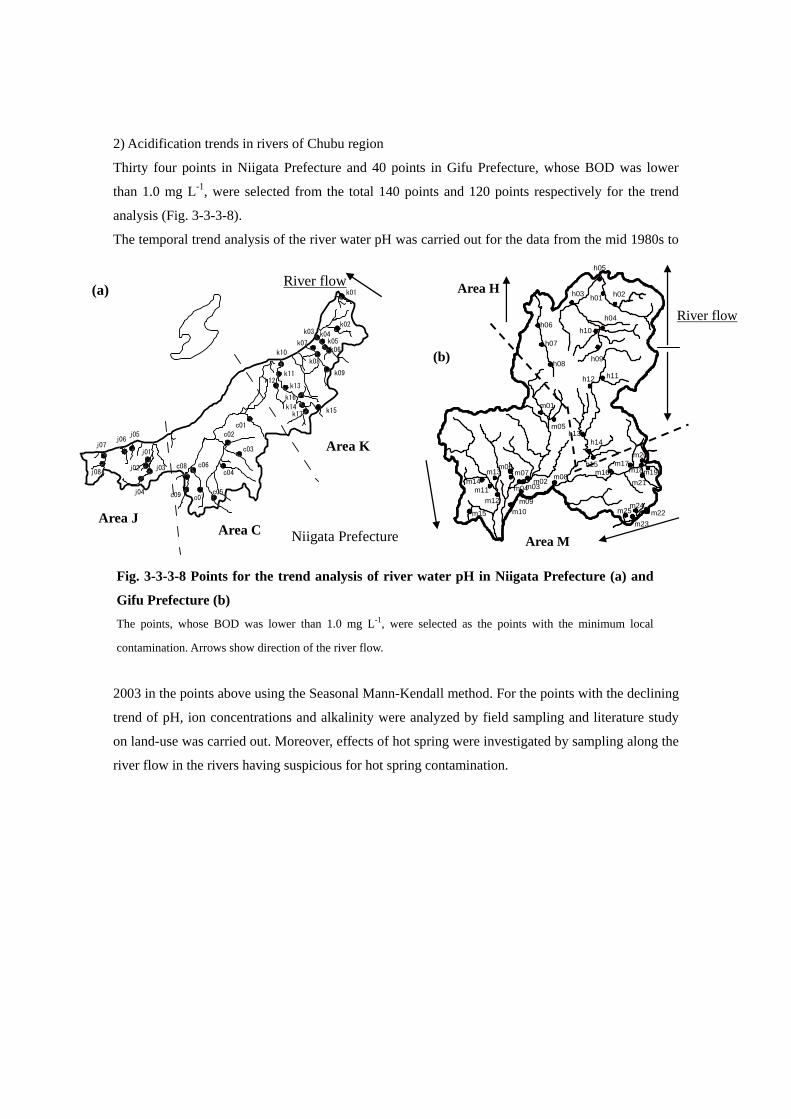
2) Acidification trends in rivers of Chubu region

Thirty four points in Niigata Prefecture and 40 points in Gifu Prefecture, whose BOD was lower

than 1.0 mg L-1, were selected from the total 140 points and 120 points respectively for the trend

analysis (Fig. 3-3-3-8).

The temporal trend analysis of the river water pH was carried out for the data from the mid 1980s to

2003 in the points above using the Seasonal Mann-Kendall method. For the points with the declining

trend of pH, ion concentrations and alkalinity were analyzed by field sampling and literature study

on land-use was carried out. Moreover, effects of hot spring were investigated by sampling along the

river flow in the rivers having suspicious for hot spring contamination.

Fig. 3-3-3-8 Points for the trend analysis of river water pH in Niigata Prefecture (a) and

Gifu Prefecture (b) The points, whose BOD was lower than 1.0 mg L-1, were selected as the points with the minimum local

contamination. Arrows show direction of the river flow.

k01

k02k03 k04

k05k06

k07

k08

k09

k10

k11k12

k13

k14k15

k16

k17

c01

c02

c03

c04

c05

c06

c07

c08

c09

j01

j02 j03

j04

j05j06

j07

j08

Area K

Area C Area J

Niigata Prefecture

(a) River flow

Area M

h05

h01 h02h03

h04

h10

h09

h06

h07

h08h11h12

h13h14

h15

m01

m05

m02m03m04

m09m10

m06m07 m08

m11m12

m13m14

m15

m16m17

m20

m21

m18

m22m23

m24

m19

m25

Area H

River flow

(b)

The long-term acidification trend of the river water pH was found by the temporal trend analysis at

11 points in Niigata Prefecture and 13 points in Gifu Prefecture as shown in Table 3-3-3-2. In

particular in Niigata Prefecture, all the points with the declining pH trend are located especially in

the northern part, area K (Ka-etsu). In Gifu Prefecture, locality of the trend was not obvious and the

declining trend was found mostly in the upstream rivers.

Note: n, number of the data; Z-score shows the trend and its strength, the positive value shows increasing trend and the negative value

shows declining trend; Hatched cells show significant declining trends.

Table 3-3-3-2 The long-term trend of the river water pH in Niigata Prefecture (a) and Gifu

Prefecture (b) (a) (b)

Area River system River name Points n ZscoreK Ou River Omata k01 213 -2.45*

Miomote River Miomote k02 213 -3.06**Ara River Aara k03 211 -4.92***

k04 215 -4.71***k05 213 -7.34***k06 215 -8.22***

Tinai River Tainai k07 205 -1.25k08 211 -2.27*k09 215 -1.42

Agano River Agano k10 213 -0.28k11 213 -0.95k12 214 -1.12k13 215 0.24k14 213 -3.53***k15 213 -3.58***

Araya k16 214 -3.31***Tokonami k17 212 -3.78***

C Shinano Ikarashi c01 214 -1.29Hama c02 213 0.13Sanashi c03 213 -0.64Mikuni c04 196 1.03Uozu c05 212 0.11Kisyosu c06 215 2.65**

c07 212 0.66Nakatsu c08 214 7.50***

c09 209 3.54***J Ski River Yashiro j01 212 0.58

Sibue j02 215 2.90**Seki j03 215 1.49

j04 214 5.50***No River No j05 215 1.08Haya River Haya j06 213 -0.95Hime River Hime j07 212 0.65

j08 214 0.38

*＝p<0.05 **＝p<0.01 ***

＝p<0.001

River system River name Point n ZscoreH Takahara River Takahara h01 191 -3.00**

h02 191 -2.99**Miya River Odori h03 96 3.24**

Kohachiga h04 191 -3.08**Miya h05 191 -1.70

Sho River Sho h06 96 -2.87**h07 64 -1.55h08 64 -1.61

Miya River Miya h09 191 -6.65***Kawakami h10 96 1.55

Kiso River Osaka h11 96 -0.78Hida h12 192 -1.68Maze h13 186 0.01Shira h14 96 5.76***Kuro h15 96 5.15***

M Western part Nagara River Nagara m01 192 3.42***m02 192 -5.78***m03 192 -3.95***m04 192 -3.77***

Yoshida m05 192 6.00***Ijira m06 192 8.53***

m07 192 0.489Kiso River Kiso m08 192 -6.28***

m09 192 -0.79m10 192 -1.48

Ibi River Ibi m11 192 -5.03***m12 192 -2.63**

Neo m13 192 -2.62**Kasu m14 188 1.27Makita m15 192 2.37*

Eastern part Kiso River Nakanokata m16 96 3.11**Tukechi m17 96 1.35Kawaue m18 96 1.39Ochiai m19 96 2.16*Kiso m20 192 0.89Nakatsu m21 96 2.98**

Yahagi River Yahagi m22 191 3.33***m23 192 -4.28***

Kamimura m24 180 2.86**Azuma m25 96 3.07**

*＝p<0.05 **＝p<0.01 ***

＝p<0.001

Area

According to the field surveys in Niigata Prefecture, alkalinity and EC were lower than 0.200 mmolc

L-1 and 10 mS m-1 respectively, suggesting their high acid sensitive, in most points of the area K,

whose upstream area was dominated by granite. On the other hand, alkalinity and EC were higher,

suggesting low acid sensitive, in area J and area C (Jo-etsu and Chu-etsu), whose upstream area was

dominated by andesite or limestone. The long-term trend of the river water pH may reflect the

bedrock geology. In Gifu Prefecture also, acid-sensitive geology, such as granite, rhyolite and chert,

can be found. Although locality of the pH trend relationship between the geology and the river water

chemistry were not obvious, the long-term declining trend of pH was observed in the upstream

points, such as h02, h09, and m11.

The river water chemistry may have large effects of land use in the watershed. Moreover, in case of

Japan, there are many volcanoes, and hot springs or mineral springs may exist in upstream area of

mountains. The investigation along the river flow near hot springs found clear effects of hot spring

on the river water chemistry in c06, c07, c08 and c09 of Niigata Prefecture and h02 of Gifu

Prefecture, in which EC and SO42- concentration increased significantly near hot springs. On the

other hand, in k01, k06, k16 and k17 of Niigata Prefecture and h09 and m11 of Gifu Prefecture, it

was suggested that effects of hot spring drainage and mines were minimum. Moreover, 90% of the

watersheds were occupied by forest and the percentage of agricultural field was significantly low in

these points.

The typical declining trends of pH in the points with minimal effects of land use and hot spring were

6

6.5

7

7.5

8

8.5

1986 1988 1990 1992 1994 1996 1998 2000 2002

pH

(a)

Fig. 3-3-3-9 Typical declining trends of pH in a) k16, Kotobukibashi Bridge in Araya

River, Niigata Prefecture and in b) m11, Okajima Bridge in Ibi River, Gifu Prefectrure

(b)

6

6.5

7

7.5

8

8.5

1988 1990 1992 1994 1996 1998 2000 2002

pH

shown in Fig. 3-3-3-9. Most points of Niigata Prefecture shows relatively monotonous declining

trend as seen in k16 of Fig. 3-3-3-9 a). In case of Gifu Prefecture, as seen in m11 of Fig. 3-3-3-9 b),

the pH declined clearly after 1996, which was similar to the phenomenon observed in the

Kamagatani River flowing into the Lake Ijira. However, slight increase can be seen after 2000,

which was different from the Kamagatani River. The upstream area of Araya River (k16) was

dominated by granite, and the area of Ibi River was dominated by sedimentary rocks including chert

and granite. As the seasonal variation, the lowest pH was recorded in Niigata and Gifu prefectures in

April or May, snow-melting season of high mountainous area,, which may reflect so-called acid

shock phenomena.

As shown in the spatial distribution of wet deposition in Japan, the area along the Sea of Japan

represented by Niigata Prefecture and Chubu region represented by Gifu Prefecture can be

characterized as the area with high wet deposition load. The trend analysis above was not a direct

evidence of acid deposition impacts on the river water chemistry. However, the natural

environmental factors such as hot spring and volcano and the anthropogenic factors such as land-use

change, agriculture and mining cannot explain adequately the long-term declining trend of pH in

several points of Niigata and Gifu prefectures. It may be possible that similar phenomena occur in

other acid-sensitive areas. Acidification of streams or rivers should be further focused on. Moreover,

similarity between the long-term declining trends in Gifu Prefecture and the trend in the Lake Ijira

should be investigated.

3.3.4 Current status of watershed acidification in Japan and future directions of the catchment

analysis

Synthesis analysis based on the previous monitoring activities and the intensive surveys suggested

that atmospheric deposition of S, N, and H+, which is the highest level among Japan, affected the

river water chemistry through biogeochemical cycles in forest ecosystems in the Lake Ijira

(Kamagatani) catchment.

Based on precise estimates of wet deposition and dry deposition, N deposition in the catchment was

significantly higher than the threshold value, , at which NO3- leaching into streams or rivers would

be accelerated in Europe and U.S. In fact, NO3- concentration in the river showed the increasing

trend and no seasonality with relatively high concentrations even in summer, when vegetation N

uptake must be active. The river pH showed declining trend. It was suggested that significant high N

deposition contributed to the river acidification. Although the trigger of the phenomena may be

meteorological events in the mid-1990s, the catchment is continuously acidified by NO3- leaching

derived from high N deposition, which may exceed the capacity of the ecosystems.

On the other hand, S output exceeded the input in the catchment. It was suggested that S

accumulated in the past was discharged from the catchment, possibly contributing to the

acidification above. Since concentrations of NO3-と SO4

2- increased simultaneously with increase of

the water discharge during heavy rain events, it was suggested that the accumulated S was

discharged with N from shallow soil layers.

The Lake Ijira catchment is a typical forested catchment in Japan, where Japanese cedar and cypress

were planted, and the similar acidic rocks are distributed in many areas. The acidification of

watersheds may not be a specific phenomenon in this area. The acid-sensitive catchment, high

deposition load, and meteorological events as a trigger functioned as the necessary conditions for the

acidification. The spatial distribution of wet deposition indicated existence of the areas with high

deposition load comparable to the Lake Ijira. In particular, in the area along the Sea of Japan in

Chubu region, the wet deposition amounts are recently the highest level in Japan. Moreover, the

long-term declining trends of the river water pH in Niigata and Gifu prefectures indicated possible

acidification of watersheds in the areas with acid-sensitive geology and high acid deposition.

As described in the section 3.2, taking these phenomena into consideration, the area with acid

sensitive ecosystems and high acid deposition should be identified as hot spots, and possible effects

of acid deposition on the river water chemistry should be investigated in further detail. Moreover,

since soil pH decreased to lower than pH 4.0 in the Lake Ijira catchment, leaching of Al3+, which is

toxic to plant growth, may increase accordingly. Continuous monitoring including effects on trees

may be necessary.

As the reasons why the acidification trends could be identified in the Lake Ijira catchment, in

addition that the area had necessary conditions as a hot spot, it can be pointed out that an integrated

monitoring including atmospheric deposition, soil, vegetation, and inland water has been

implemented here. The catchment-scale analysis of biogeochemical material cycles may allow more

quantitative discussion on effects of acid deposition on forest ecosystems. For further development

of the catchment-scale analysis as the integrated monitoring in future, the following subjects should

be discussed.

1) Strengthening of the stream/river monitoring and promotion of catchment analysis

The monitoring on streams and rivers should be more focused on, which may reflect changes

in material cycles more directly. Taking hot spots into account, widespread information

should be accumulated. As for the Lake Ijira catchment, monitoring in the Kamagatani River

will be carried out continuously at two-week interval, and the long-term assessment of the

river water chemistry and input-output budget will be carried out. In future, more effective

monitoring methodologies should be discussed with development of the catchment-scale

model.

2) Development of effective methods to estimate forest growth and nutrient uptake

Tree growth and nutrient uptake may be closely related to acidification of the catchment as

discussed above. To evaluate acidification derived from external H+ sources such as acid

deposition quantitatively, it is important to estimate plant growth and nutrient uptake in the

whole forest area. The precise estimation of forest growth requires detailed and continuous

field observations. In future, more effective and simplified estimation methodologies should

be developed for the catchment analysis.

3) Collaboration with existing study sites

Research outcomes in existing study sites managed by universities and research organizations

should be referred for further collaboration between the Long-term Acid Deposition Surveys

and the research activities. Cooperative intensive observations or standardization of the

monitoring methodologies should be promoted. In future, synthesis assessment of Japanese

watersheds including the Lake Ijira catchment should be discussed. Through the assessment,

the position of the catchment analysis should be clarified in the Long-term Acid Deposition

Surveys.

4) Dissemination of the catchment analysis to the East Asian region

The catchment analysis will be an effective tool for assessment of ecological impacts in the

East Asian region, where emission of acid substances is being increased. Studies of the

catchment analysis should be promoted in the region.

5) Development of the catchment-scale model

Quantitative data obtained through the intensive surveys, the data in existing study sites in

Japan, and case studies in the East Asian region should be integrated for development of the

catchment-scale model including comparison of existing models. For validation of the

acidification mechanism in the Lake Ijira catchment, modeling may be essential. The data

obtained by 1) and 2) above will be informative as validation data of the model.

Taking the subjects into account, the catchment-scale analysis should be promoted as the integrated

monitoring and assessment methodologies for impacts of acid deposition on ecosystems.

References

1) Kobayashi J. 1960. A chemical study of the average quality and characteristics of river waters of

Japan. Berichte des Ohara Instituts fuer Landwirtschaftliche Biologie Okayama Universitaet 11:

313-358.

2) Nakahara, O., Takahashi, M., Sase, H., Yamada, T., Matsuda, K., Ohizumi, T., Fukuhara, H.,

Inoue, T., Takahashi, A., Kobayashi, H., Hatano, R., Hakamata, T. 2008. Stream water

acidification and increasing NO3– discharge in a forested catchment in central Japan (submitted).

3) Kurita H., Ueda, H. 2006. Long-term decrease of pH of river and lake water in the upper-most

stream part of the mountainous region in central Japan – Decrease of pH in past 30 years in

relation with Acid Rain. J. Jpn. Soc. Atmos. Environ. 41(2): 45-64 (in Japanese).

4) van Breemen, N., Mulder, J. Driscoll, C.T. 1983. Acidification and alkalinization of soils. Plant

and Soil 75: 283-308.

5) Tokuchi, N., Ote, N. 1998. H+ budget in the forest ecosystems. Japanese Journal of Ecology 48:

287-296 (in Japanese).

6) Matsubara, M., Morimoto, S., Sase, H., Ohizumi, T., Sumida, H., Nakata, M. Ueda, H. 2008.

Long-term declining trends of river water pH in Central Japan. Water Air Soil Pollut (in press).

doi: 10.1007/s11270-008-9909-3

3.4 Comparison with foreign monitoring data EANET was established in 1998 and started its regular phase of operation in 2001. The

monitoring results were reported every year as the data report. In 2007, “Periodic Report in the State

of Acid deposition in East Asia”1) was published, which described the outcomes of five-years’ EANET’s monitoring activities(2000-2004), and was the first report with comprehensive analysis

and assessment of acid deposition in East Asia.

The European continent has long been covered by the Co-operative Programme for Monitoring

and Evaluation of Long-range Transmission of Air Pollutants in Europe (EMEP), and the monitoring

in North American region has been also continuously conducted by the National Atmospheric

Deposition Program (NADP) etc.

In this section, the state of acid deposition in Japan was compared with those in East Asia, Europe

and North America using these monitoring data above mentioned.

3.4.1 Atmospheric deposition

(1) State of wet deposition

The state of wet deposition in Japan, East Asia, North America and Europe was analyzed. The

data in non-urban sites of this survey in Japan and the data in non-urban sites of Acid Deposition

Survey conducted by Japan Environmental Laboratories Association2)～5) were used for comparison

with EANET6), NADP7), and EMEP8) data, which represent the data in East Asia, North America,

and Europe respectively. The data that satisfy the completeness (%TP and %PCL) above 80% during

the period from April 2003 to March 2007 for Japan and from January 2003 to December 2007 for

other regions were used for the calculation of annual means.

Figure 3-4-4-1 shows the relationships between ion concentrations and precipitation amounts of

10, 25, 50, 75, and 90 percentiles on deposition flux in Japan, North America, and Europe. The range

of precipitation amounts in Japan were larger than those in North America and Europe, and the

median value in Japan was 1680mm y-1, which was 1.7 times larger than in North America and 2.5

times than in Europe. nss-SO42- concentrations in Japan were distributed in narrow range with high

concentrations compared with Europe and North America, and the 10 percentile value was the same

concentration of the median value in Europe and North America. The median concentration in Japan

was 1.6 times higher than in North America and 1.3 times in Europe. Median value of deposition

amounts of nss-SO42- in Japan exceeded 20 mmol m-2, which was three times larger than in Europe

and North America. The range of NO3- concentrations in Japan and North America were within those

in Europe, and the median value in Europe was the highest among the three regions and that of Japan

was about 70% of Europe. However, because of large precipitation amounts, deposition amounts of

NO3- in Japan was about two times larger than those in Europe and North America.

Acidity of rain water in Japan were distributed in narrower range than in Europe and North

America. The range of pH values in Japan were the latter half of 4. However pH values in Europe

and North America were distributed between middle of 4 and middle of 5, which were wider range

than in Japan. The median pH value was 4.7 in Japan, 4.9 in North America and 5.0 in Europe,

which mean the concentration of H+ in Japan were 1.7 times and 2.2 times higher than in North

America and Europe, respectively. Therefore the median value of H+ deposition amounts in Japan

was 6 times and 3 times larger than in North America and Europe, which could be explained by

considering the difference of the concentrations of acidity and precipitation amounts. Furthermore,

the difference between Japan and North America, Europe could be considered the difference of

neutralization in rain water between them. It was suggested that the ratio of the neutralization of rain

water in Japan was lower than that in North America and Europe.

Figure 3-4-1-2 shows the same relationships by adding the data of monitoring sites in East Asia.

There were considerable variations of value between each site, and so mean concentration and mean

precipitation amount were used for the plot in this figure with no statistical procedures. High

concentrations of nss-SO42- were observed in China with highest concentration more than 150µmol

L-1, which was three times higher than the median value in Japan. Precipitation amounts in China

were relatively low, however deposition amounts were six times larger than the median value in

Japan due to high concentrations in China.

Relatively large deposition amounts, which were upper range of deposition amounts in Japan,

were also observed in Korea, Indonesia, Viet Nam. NO3- deposition amounts in China, Korea and

Indonesia were over the range of those in Japan. These areas were relatively low precipitation

amounts, however because of high concentration in China and Indonesia the deposition amounts

were 2 times larger than the median value in Japan.

In spite of high deposition amounts of acidic substances in East Asia, the level of acidity in rain

water and H+ deposition amounts were below the range of those in Japan. It was suggested that the

ratio of the neutralization of rain water in East Asia region was higher than that in Japan.

日本

北米

nss-

SO42-

欧州

10

50

3

30

0

10

20

30

0 500 1000 1500 2000 2500 3000 3500

年降水量（mm y-1）

年平

均濃

度（

μmol

L-1）

年沈

着量

（m

mol m

-2）

Fig.3-4-1-1 Wet deposition amounts in Japan and comparison with the data in Europe and North America(2003-2006)

1) Japan: JPN, n=68, North America: NADP, n=250, Europe: EMEP, n=97 2) Black points Dot point shows 10, 25, 50, 75, and 90 percentiles of ion concentration and precipitation amounts in Japan, North America, and Europe.

日本

NO3-

北米

欧州

10

30

50

30

10

20

30

40

0 500 1000 1500 2000 2500 3000 3500


年平

均濃

度（

μmol L

-1）

年沈

着量

（m

mol m

-2）

日本

H+

北米

欧州

10

30

100

50

70

31

10

100

0 500 1000 1500 2000 2500 3000 3500


年平

均ｐ

H

H+年

沈着

量（m

mol m

-2）

6.0

5.0

4.0

年

沈着量（

mmol m-2 ）

年沈着量（

mmol m-2 ）

年沈着量（

mmol m-2 ）

JPN

JPN

JPN

NADP

NADP

EMEP

NADP

EMEP

EMEP

Annual

mean

conce

ntr

atio

n／

µm

ol L

-1

Annual

mean

conce

ntr

atio

n／

µm

ol L

-1

Ann

ual d

epos

ition

rat

e／m

mol

m-2

A

nnua

l dep

ositi

on r

ate／

mm

ol m

-2

Ann

ual d

epos

ition

rat

e／m

mol

m-2

Annual precipitation rate／mm y-1

Annual

mean

pH

val

ue

Fig.3-4-1-2 Wet deposition amounts in East Asia and comparison with those in Japan, Europe and North America(2003-2006)

1) Japan:JPN, n=68, North America:NADP, n=250, Europe:EMEP, n=97 2) East Asoa: ○:China, ▲:Indonesia, ●:Malaysia, □:Mongolia, △:Philippines, ■:Korea、

×:Russia, ＋:Thailand, ＊:Viet Nam

日本

北米

欧州

nss-

SO42-

10

100

300

30

31

10

100

1000

0 500 1000 1500 2000 2500 3000 3500


年平

均濃

度（

μmol L

-1）

年沈

着量

（m

mol m

-2）

日本

北米

欧州

NO3-

10

30

50

70

30

10

20

30

40

50

60

0 500 1000 1500 2000 2500 3000 3500


年平

均濃

度（

μmol L

-1 ）

年沈

着量

（m

mol m

-2 ）

日本

北米

欧州

H+

10

30

50

70

3

100

1

10

100

0 500 1000 1500 2000 2500 3000 3500


年平

均 p

H

H+年

沈着

量（m

mol m

-2）

5.0

4.0

6.0

年沈着量（mmol m-2 ）



JPN

JPN

JPN

NADPEMEP

NADP

NADP

EMEP

EMEP

Annual

mean

conce

ntr

atio

n／

µm

ol L

-1

Ann

ual d

epos

ition

rat

e／m

mol

m-2

Annual

mean

conce

ntr

atio

n／

µm

ol L

-1

Ann

ual d

epos

ition

rat

e／m

mol

m-2

A

nnua

l dep

ositi

on r

ate／

mm

ol m

-2

Annual precipitation rate／mm y-1

Annual

mean

pH

val

ue

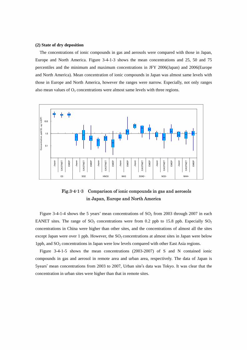
(2) State of dry deposition

The concentrations of ionic compounds in gas and aerosols were compared with those in Japan,

Europe and North America. Figure 3-4-1-3 shows the mean concentrations and 25, 50 and 75

percentiles and the minimum and maximum concentrations in JFY 2006(Japan) and 2006(Europe

and North America). Mean concentration of ionic compounds in Japan was almost same levels with

those in Europe and North America, however the ranges were narrow. Especially, not only ranges

also mean values of O3 concentrations were almost same levels with three regions.

Fig.3-4-1-3 Comparison of ionic compounds in gas and aerosols in Japan, Europe and North America

Figure 3-4-1-4 shows the 5 years’ mean concentrations of SO2 from 2003 through 2007 in each

EANET sites. The range of SO2 concentrations were from 0.2 ppb to 15.8 ppb. Especially SO2

concentrations in China were higher than other sites, and the concentrations of almost all the sites

except Japan were over 1 ppb. However, the SO2 concentrations at almost sites in Japan were below

1ppb, and SO2 concentrations in Japan were low levels compared with other East Asia regions.

Figure 3-4-1-5 shows the mean concentrations (2003-2007) of S and N contained ionic

compounds in gas and aerosol in remote area and urban area, respectively. The data of Japan is

5years’ mean concentrations from 2003 to 2007, Urban site’s data was Tokyo. It was clear that the

concentration in urban sites were higher than that in remote sites.

0.0

0.1

1.0

10.0

Japan

CA

STN

ET

EM

EP

Japan

CA

STN

ET

EM

EP

Japan

CA

STN

ET

EM

EP

Japan

EM

EP

Japan

CA

STN

ET

EM

EP

Japan

CA

STN

ET

EM

EP

Japan

CA

STN

ET

EM

EP

O3 SO2 HNO3 NH3 SO42- NO3- NH4+

Concentr

ation, p

pb(G

), u

g/m

3(P

)

0 5 10 15 20

SerpongPetaling Jaya

Tanah RataChiangmai

KhanchanaburiPatumthani

SamutprakarnBangkokHoa Binh

Ha NoiLos Banos

Metro ManilaOgasawara

HedoYusuhara

BanryuOkiIjira

HappoSado-seki

TappiRishiri

ImsilCheju

KanghwaZhuhai

XiamenChongqing

TereljUlaanbaatarPrimorskaya

IrkutskListvianka

Mondy

IDM

YTH

VNPH

JPKR

CNM

NRU

Concentration/ ppb

ID Serpong

JP Banryu

JP Oki

図3-4-1-4 SO2 concentrations in EANET sites (2003-2007) Monitoring were carried out by automatic monitors and filter-pack method

Rural SiteUrban Site

RemoteSite

NO3-(P)/HNO3(G)

SO42-(P)/SO2G)

NH4+(P)/NH3(G)

(i) Remote Sites

(ii) Urban Sites

図 3-4-1-5 Air concentrations of S and N contained compounds in gas and aerosols in Japan and East Asia ( Unit: nmol m-3)

nmol m-3

3.4.2 Impacts on ecosystems

(1) Soil acidification

Soil has acid buffering capacity and acidification proceeds gradually with several steps. Therefore,

short-term monitoring or temporary surveys mostly cannot detect small changes in soil chemical

properties.

In EANET, the soil surveys have been done only once or twice in most sites, and it is impossible to

evaluate soil acidification status only by the EANET data. However, in case of Lake Ijira catchment,

one of the EANET monitoring sites, soil surveys have been conducted continuously by the Japanese

Acid Deposition Surveys since 1988, and a soil acidification process was able to be detected there.

At present, the soil acidification in Lake Ijira catchment is only one case, which may be attributed to

acid deposition.

In Europe, the International Co-operative Programme on Assessment and Monitoring of Air

Pollution Effects on Forests (ICP Forests) under the UNECE Convention on Long-range

Transboundary Air Pollution started large-scale soil surveys at 5,300 plots since 1994. The second

surveys are now being conducted in the respective countries. Therefore, chronological changes in

soil chemical properties in European scale will be reported in near future. However, in Europe, soil

acidification has been reported in several forest areas. A case in Southeast Sweden may be the most

famous as a long-term acidification of soil. In this case, the area, which was originally surveyed in

1927, was surveyed again from 1982 to 1984, after 55 years from the first survey, and then, the soil

acidification phenomena were obviously detected there.

(2) Tree decline

The current situation on tree decline symptoms in the EANET monitoring sites was shown in Fig.

3-4-2-1. Tree decline symptoms were reported in most monitoring sites. Especially in Dabagou of

China, and Bolshie Koty and Irkutsk of Russia, all the trees showed some decline symptoms.

Possible causes of the tree decline were presumed to be disease or insects in most sites and

meteorological or topographical conditions in some sites. However, the cause was also not identified

clearly in many sites. In Irkutsk, where the cause was not identified, local scientists suggested that

effects of air pollution derived from industrial area around Baikal Lake.

In addition to the monitoring sites above, decline of larch (Larix sibirica) trees was reported in

Bogdkhan Mountain near Ulaanbaatar City, the capital of Mongolia (Fig. 3-4-2-2). Effects of SO2

and other acidic pollutants derived from coal combustion in thermal power plants or mobile houses

(Ger) were suggested as one of possible cause of the tree decline. Since the city of Ulaanbaatar is

located in a basin surrounded by mountains, air pollutants will be still in the basin especially in

winter. Airborne particulate matters could be detected visually in the city area and the slopes of

Bogdkhan Mountain were smoggy in winter. Sulfur concentrations of larch needles were twice in the

Fig. 3-4-2-2 Decline of larch trees in Mt. Bogdkhan near Ulaanbaatar City The photo was taken on the slope facing the Thermal Power Plant NO.3.

Fig. 3-4-2-1 Tree decline symptoms observed in the EANET sites

Based on the observation from 2000 to 2004; number of trees: 20 (at least 12); cn, China; jp, Japan;

ph, Philioppines; kr, Republic of Korea; ru, Russia, th, Thailand (EANET, 2006）

010

203040

5060

708090

100

% o

f dec

lined

tree

s

Jinyu

nshan

No.1

Jinyu

nshan

No.2

Dabag

ou

XPZ-01

XPZ-02

XPZ-03

XPZ-04

Zhuxia

ndon

g No.1

Zhuxia

ndon

g No 2

Zhuxia

ndon

g No 3

Lake I

jira

Yamato

Banryu

Iwam

i-rink

u FP

Mt. Mak

illing

UP Que

zon-L

and G

rant

Mt. Naej

ang

Bolshie

Koty

Irkuts

k

Mondy

Vachira

longk

orn Puy

e

Vachira

longk

orn D

am

natural factors unknown factors insect or disease

cn jp ph kr ru th

slope facing a thermal power plant than in reference forests (approx. 2mg-S g-1).

As described above, tree declines reported in the EANET countries were mainly caused by relatively

local air pollution. In many cases of Japan also, the tree decline symptoms were reported around big

cities, such as decline of Cryptomeria japonica in Kanto Plain (mainly in Saitama next Tokyo) and

tree decline in Nikko or Akagi (Tochigi or Gunma, downwind direction of Tokyo). So far, effects of

transboundary air pollution on tree decline have not been reported.

On the other hand, recently, ozone concentrations have increased gradually, and the Photochemical Oxidants Warning has been issued in wider areas. As one of the possible causes of the high ozone concentrations, transboundary air pollution from the Asian Continent is pointed out. The annual mean ozone concentrations were higher than 60 ppb in higher altitudes, such as Akagi and Happo-One, and higher than 40 ppb in islands or coastal area along the Sea of Japan, such as Tappi Point, Sado-Seki Point, Oki Island, and Tsushima Island (see the section 3.1.2). In other East Asian countries, high ozone concentrations have been reported. The mean ozone concentrations of wet and dry seasons in a tropical seasonal forest in Thailand were shown in Table 3-4-2-1. The values shown here were 15-day mean values obtained by the Ogawa passive sampler. The maximum concentration was higher than 60 ppb and the mean concentration in dry seasons were higher than 40 ppb. Accumulated exposure over a threshold of 40 ppb (AOT40) is used as an indicator of plant growth in Europe. High ozone concentrations in forest area and their effects on plant should be monitored in detail.

Table 3-4-2-1 Ozone concentrations in a tropical seasonal forest, in Sakaerat Silvicultural Research

Station, Thailand

Year Season Mean Median Minimum Maximum

2005-2006 Dry (Dec - Mar) 43.0 40.6 29.7 64.2

2006 Wet (Apr - Nov) 29.2 25.6 19.8 66.7

2006-2007 Dry (Dec - Mar) 45.5 43.0 34.0 58.1

Note. The ozone concentrations above show the 15-day mean values obtained by the Ogawa passive sampler.

In Europe, ICP Forests started the surveys on ozone effects, including the measurement of ozone

concentrations in forest area by passive samplers and observation of ozone visible injury. According

to test phase of the passive sampling, the mean concentrations were higher than 45 ppb in many

Mediterranean countries such as Italy and Spain.

(3) Inland water acidification

In EANET, acidification trends of inland water have not been reported. Acid-sensitive lakes, whose

alkalinity is lower than 0.200 mmolc L-1 and EC is lower than 10mS m-1, were found in China, Japan,

and Russia. However, most monitoring sites in Southeast Asian countries did not meet the criteria

above. It is difficult to find appropriate lakes in East Asian countries and acid buffering mechanisms

of lakes are quite complicated. Rivers, which may directly reflect material cycles in the catchments,

will be selected as the monitoring site in near future in EANET.

In Europe, the International Cooperative Programme on Assessment and Monitoring of Rivers and

Lakes (ICP Waters) has promoted wide-range monitoring of inland waters. As the emission was

reduced in Europe, SO42- concentrations in rivers and lakes have been reduced year by year, and the

reduction rate was the largest in 1990s. While SO42- leaching was regulated by S deposition, NO3

-

concentrations in the inland waters did not show any clear trends and it was suggested that leaching

processes of N may be more complicated. Alkalinity did not change at two-third of the sites but

increased at one-third of the sites. From 1990 to 2001, acidification still proceeded at 14% of the

sites. However, it was reported that acidification may not proceed in Europe from now on. Thus,

inland waters in Europe may be in a process of recovery from acidification.

On the other hand, in Japan, the Synthesis Report of Japan Acid Deposition Surveys reported

acidification trends in rivers and lakes in mountainous areas with low acid buffering capacity and

acid shock phenomena in snow-melting seasons. Moreover, in this report, not only in Lake Ijira, but

also in widespread area of Niigata Prefecture and Gifu Prefecture, acidification of rivers was

reported. Therefore, in East Asia including Japan, effects of acid deposition on inland waters should

be monitored continuously.

（引用文献）

1) EANET, 2006. Periodic Report on the State of Acid Deposition in East Asia, Part I: Regional

Assessment and Part II: National Assessment. http://www.eanet.cc/product.html

2) 全国環境研協議会、第４次酸性雨全国調査報告書（平成 15 年度）、全国環境研会誌、30(2)、

19-37、2005


13-33、2006


3-31、2007


2-72、2008

6) Network Center for EANET, Acid Deposition Monitoring Network in East Asia (EANET) Data

Report 2003, 2004, 2005, and 2006.

7) NADP, 2008. Data access. National Atmospheric Deposition Program (NADP), http://nadp.sws.uiuc.edu/sites/ntnmap.asp?

8) EMEP, 2008. EMEP measurement online. EMEP Chemical Coordinating Centre at NILU, http://www.nilu.no/projects/ccc/emepdata.html

9) Hallbäcken & Tamm, 1986. Changes in soil acidity from 1927 to 1982-1984 in a forest area of

south-west Sweden. Scand. J. For. Res. 1: 219-232. 10) Sase H., Bulgan T., Batchuhuluun T., Shimizu H., Totsuka T. 2005. Tree decline and its

possible causes around Mt. Bogdkhan in Mongolia. Phyton (Horn, Austria) 45: 583-590.

4. Long-Range Trans-boundary Air Pollution

The term ”Trans-boundary Air Pollution” can be traced back to the 1960s, when

acidification phenomenon became serious environmental issues in Europe. When the

interrelationship between sulfur emissions in continental Europe and the acidification in

Scandinavian lakes were recognized as serious environmental problems, it was pointed

out by Swedish meteorologist that air pollutants including acidic substances could be

transported over long-range from Europe continent and UK1). After that, in accordance

with worse condition on acidification phenomenon in Europe and boundary area between

UAS and Canada, research on long-range transportation of acidic substances developed

dynamically from 1970s to 1980s in Europe and North America2). During these decades,

the Convention on Long-Range Trans-boundary Air Pollution (CLRTAP) was adopted in

1979 with the participation of European countries including USSR(Russia), USA and

Canada. Since then, control measures to reduce emissions of sulfur and nitrogen oxides

were enforced, and acidification phenomenon did not become so serious problems in

1990s.

Instead of acidification phenomenon, increasing of ozone concentrations was beginning

to appear as environmental issues. In Europe and North America, counter measures for

nitrogen oxide and VOC conducted properly, however ozone concentrations did not

achieve the environmental standards levels. Possible causes of these results included the

increasing of the back-ground ozone concentrations in northern hemisphere, and to

achieve the environmental standards, it was necessary to address the ozone issue as a

hemispheric issue and to discuss internationally. Taking above mentioned matter into

account, the Task Force on Hemispheric Transport of Air Pollution(TF-HTAP) was

established(ref. 4.4.1) under CLRTAP.

Meanwhile, in East Asia concern about acidification phenomenon arose after 1990s,

and the Acid Deposition Monitoring Network in East Asia(EANET) was established.

Same time, transportation of acidic substances in East Asia became a matter of concern,

and the contribution of sulfur oxide in Japan from China and Korea etc. were examined

and reported3). However, the results of the calculation varied widely and impact caused by

acidification phenomena was considered as the issues of long-term risks.

Same as Europe, ozone issue became of interest lately in East Asia. In Japan, in spite of

the decrease of the atmospheric concentration of precursor pollutants, VOC and NOx,

long–term increasing trend of ozone concentrations has been shown. Then increasing

ozone concentrations in China accompanied with rapid economic growth and the effect of

trans-boundary air pollutants to Japan began to investigate. On the one hand, it became

clear that hemispherical air pollution of ozone caused by the inter-continental

transportation affected the increasing of back-ground ozone concentrations and related

deeply with the difficulty of the achievement of environmental standard. Therefore, it is

necessary to discuss the ozone control measures of Japan in future taking international

framework into account, which includes the transportation issues in East Asia region and

the inter-continental and hemispherical transport of air pollution.

4.2 The Increasing Emissions of Air Pollutants in East Asia Using the emission inventory for Asia(Regional Emission inventory in Asia, REAS)４)

emission trends between 1980 and 2003, and projections of future emissions of air pollutants(NOx, SO2, NMVOC) in East Asia are presented here. (i) Yearly emission changes of air pollutants

Figure 4-1 shows the yearly changes of regional emissions in the period 1980-2003. Also shown in table 4-1 are emission amounts in 1980, 1990 and 2003 in East Asia. Total emissions of NOx in Asia were 25.11 million tons in 2000 and China and India occupied 45% and 19% respectively. In China, the country with the largest emissions, coal-burning power plants were the largest emitters(34%), followed by industrial coal use and transport oil use(both at 25%). From 1980 to 2003, fuel consumption increased 2.3 times and NOx emissions also increased 2.8 times in Asia. However in China NOx emissions increased 3.8 times, yearly average 6%, during same period, and recently increased 3 times in 3 years after 2000, which were the highest record in China.

Total Asian emissions of SO2 were 41.49 Mt in 2000, and 64% of them were discharged from coal combustion facilities in factories and power plants etc. From 1980 to 2003, SO2

emissions increased 2.2 times in Asia, 2.1 times in East Asia, and 2.5 times in China. Then, emissions of NMVOC in Asia were 40.24 million tons, in which combustion facilities of factories and power plants occupied 38% and transportation, automobiles etc.,33%. From 1980 to 2003, emissions of NMVOC increased 2.1 times in Asia, 2.4 times in East Asia, and 2.5 times in China. (ii) Future emission trends of air pollutants

Future projection of Asian emission was performed on the basis of emission scenarios and emissions for 2020 shown in table 4-2. Here, three emission scenarios for China have been developed taking into account of the trend of future energy consumption and environmental counter measures as follows; Policy Failure Case scenario(pessimistic scenario with high emission rates caused by continuation of the current energy structure, increased energy consumption, and the slow deployment of new energy technologies and new emission control technologies: PFC), Reference Case scenario (sustainable scenario with moderate emission rates caused by the suppression of energy consumption through energy conservation, a change to clean energy, and the moderate deployment of new energy technologies and new emission control technologies: REF), and Policy Succeed Case scenario (optimistic case with low emission rates owing to the implementation of

strong energy and environmental policies and the fast deployment of new energy technologies and new emission control technologies: PSC). Each concept – PSC, REF, and PFC – resembled that of the B1 scenario, the B2 scenario, and the A2 scenario of IPCC, respectively5). For other countries other than China, fuel consumption was calculated on the basis of Reference Scenario Projections in the “World Energy Outlook”(IEA).

In China, NOx emissions under the REF scenario and PFC scenario were projected to increase by 39% and 128% respectively in 2020 compared with 2000 emissions, showing only a small decrease under the PSC scenario. However, considering the increasing trends of emission and fuel-consumptions from 2000, and recent satellite observations, present NOx emissions have accelerated impressively more than the predicted values of the PFC scenario in 2020(ref. figure 4-2a).

SO2 emissions in Asian countries were projected to increase from 2000 to 2020. Emission in China showed 28% decrease in the PSC scenario, 3% decrease in the REF scenario, and 163% increase in the PFC scenario for 2020 compared 2000. 2020 NMVOC emissions in China would rapidly increase by 97%, 139%, 163% from 2000 in the PSC, REF and PFC scenario, respectively.

Table 4-1 Comparison of estimates emissions in East Asia, 1980-2003,

and increasing ratio from 1980 in parentheses.

Unit : Mt yr-1

China 3.8 6.6 (1.7) 14.5 (3.8)Other East Asia 3.6 3.8 (1.1) 4.7 (1.3)East Asia Total 7.4 10.4 (1.4) 19.2 (2.6)



Region 1980 1990

NMVOC

NOx

SO2

2003

0

5

10

15

20

25

30

1980 1985 1990 1995 2000

NO

x [M

t yr-1

]

year

Other South Asia IndiaSoutheast Asia Other East AsiaJapan China

0

10

20

30

40

50

1980 1985 1990 1995 2000

SO

2[M

t yr-1

]

year


0

10

20

30

40

50

1980 1985 1990 1995 2000

NM

VOC

[Mt y

r-1]

year


Table 4-2 Comparison of East Asian emissions in 2000, 2020

and increasing ratio from 2000 in parentheses.

Unit: Mt yr-1

Fig.4-1 Temporal evolution of emissions for NOx, SO2, NMVOC in Asia

China 11.2 11.0 (1.0) 15.6 (1.4) 25.5 (2.3)Other East Asia 4.4 5.5 (1.3) 5.5 (1.3) 5.5 (1.3)East Asia Total 15.6 16.5 (1.1) 21.1 (1.4) 31.0 (2.0)



NOx

SO2

NMVOC

Region 20002020

PSC REF PFC

REAS：Regional Emission inventory in Asia REAS_PSC：Policy Succeed Case scenario REAS_REF：Reference Case scenario REAS_PFC：Policy Failure Case scenario GOME/SCIAMACHY：NO2 column concentration measured by GOME/SCIAMACHY９) SEPA：Prediction calculated by the State Environmental Protection Administration, China (now Ministry of Environmental Protection)

a)

b)

c)

Fig. 4-2 Time series of NOx, SO2, NMVOC in China. Y axis shows the emission ratio of air pollutants to year 1996

REAS REAS_PSC REAS_REF REAS_PFC Zhang et al.(2007)6) Hao et al.(2002)8) Tian et al.(2005)7) GOME/SCIAMACHY9)

REAS REAS_PSC REAS_REF REAS_PFC Streets et al.(2000,2003)10),11) SEPA

Year

Year

Year

NOx (Ratio to year 1996)

NMVOC (Ratio to year 1996)

SO2 (Ratio to year 1996)

4.3 Effect on trans-boundary air pollution in Japan

4.3.1 State of trans-boundary air pollution in Japan (1) Ozone (i) Air pollution of ozone in East Asia O3 concentration in East Asia were simulated using the Community Multi-scale Air Quality(CMAQ) model14) and the emission inventory for Asia(Regional Emission inventory in Asia, REAS)13) for considering the spatial and seasonal variation and the contribution of regional emissions15). Figure 4-3 compares daily averaged simulated O3 concentrations with daily averaged observed O3 concentrations at Tsushima and Oki monitoring sites in 2000. O3 concentrations over Japan are controlled by two meteorological factors, the regional-scale airflow and the solar radiation, and the characteristics of ozone concentrations in this area are as follows; (i)During spring to early summer, O3 concentrations increase caused by the

increase in photochemical O3 production following the increase in solar radiation and temperature.

(ii)During summer season, O3 concentrations are lowest over year because of the penetration of clean marine air mass.

(iii)In autumn, O3 concentrations increase again because of the weakness of clean marine air mass.

(iv)In winter, O3 production is suppressed by weak solar radiation and low temperature

The solar radiation and the temperature control photochemical O3 production,

and the changes of airflow controls whether the polluted continental or cleaner marine air masses cover this area15), which phenomena can be confirmed using model analysis. Figure 4-4 illustrates 2-month, from May to July and June to

Fig.4-3 Observed (black lines) and simulated (gray lines) daily ozone concentrations at Tsushima and Oki monitoring sites in Japan15). ”R=” means each correlation coefficient between observed and simulated concentrations.

Oki Tsushima

August, averaged O3 concentration using CMAQ model. In May to July, high O3

concentrations cover China, the Korean Peninsula and Japan at around 35-40N, and the concentrations of surface O3 in the North China Plane are 65-70ppbv, and that in Northeast China, the Korean Peninsula, and a part of Japan reach 60-55ppbv. Then in summer, from July to August, the southern parts of China, the Korean Peninsula and Japan are under an effect of marine air masses, and thus O3 concentration decrease. However, the northeastern parts of China, especially North China Plane, are covered with high O3 concentrations of more than 60 ppbv. To determine the contribution of trans-boundary transported O3 to total O3, a model

run which all emissions in the model domain were turned off, zero emissions, was carried out and the dominant factors controlling the O3 concentrations over East Asia was investigated by comparing the chemically produced O3 by regional emissions and the inflow from outside of this model domain. Figure 4-5 shows the surface O3

concentrations averaged over 2 months and chemically produced by the regional emissions over East Asia including Japan, and its contribution to the total O3 concentration averaged over 2 months. From May to June, the O3 concentrations chemically produced by the regional emissions over East Asia including Japan reach 20-35 ppbv in the southern parts from Kanto area of Japan, and reach 10-25 ppbv in Honsyu island from June to August. During spring to early summer, O3 concentrations increase caused by the increase in photochemical O3 production following the increase in solar radiation and temperature. The contribution to the surface O3 concentrations (figure 4-4) is less than the concentrations chemically produced by the regional emissions over East Asia because of the outflow from outside of East Asia..

Fig. 4-4 Spatial distribution of O3 concentrations (ppbv) in 200215)

(ii) Effect to Asia from other regions

Using global chemical transport model, the extent of impacts over Eurasia from Europe and North America on ozone concentration were investigated16). The European and North American influence to Mondy in east Syberia, which represents the inflow to east Asia across Eurasia, were 0.5-3.5ppbv and 1.2-3.3 ppbv respectively. Their impacts increase in Winter and Spring, and after reaching maximum concentrations, they decrease in Summer. It was concluded that contribution ratio from Europe and North America to clean area in East Asia are totally 15%. We examined the contributions from various source regions to global distributions and budgets of tropospheric ozone (O3) in the context of intercontinental transport, using tagged tracer simulation with a global chemical transport model17). As for the impacts from Europe to East Asia, their contribution to Kagoshima was 2-2.5ppbv in April and below 1 ppbv in June, and in the case from North America to Japan, it was 1-2 ppbv in April and below 0.5 ppbv in June. Comparing the contribution of Europe and North America, there is a large contribution from Chinese planetary boundary layers (PBL) with a peak larger than 15 ppbv in spring. In summer O3 from the Asian free troposphere increases and so total contribution also reachs 15 ppbv. Contributions of 10-15 ppbv from the stratosphere in winter and spring were calculated. (iii) Transportation of the regional scale pollution in East Asia and their contributions O3 concentrations in the different air masses, regionally polluted continental air

masses (RPC) and the background continental air mass (BK),were identified using trajectory analysis and O3 data observed at Oki and Happo18). Figure 4-6 shows

Fig. 4-5 Spatial distributions of chemically produced O3 by East Asia emissions (ppbv) in 200015)

seasonal variations of O3 concentrations in the regionally polluted continental air masses, the background continental air mass, and the regional scale pollution in East Asia (EA), which were calculated by subtracting BK from RPC. O3 concentration increases in the regionally polluted continental air mass increases in spring and summer, and average concentrations from April to September was about 55 ppbv. O3 concentration in the regionally polluted continental air mass showed maximum concentrations in May, and average concentration is over 60 ppbv. These shows that monthly average O3 concentrations in the air mass transferred from continent to Japan are almost 60ppbv, environmental standards in Japan, in terms of photochemical oxidants. Seasonal variations that O3 concentrations in the regional pollution in East Asia showed maximum concentration in June –July, ranging 15-20 ppbv, and minimum in Winter, a few ppbv, were observed.

Figure 4-7 shows the monthly mean distributions of surface O3 in April 2002 and regional build-up O3 contribution from major anthropogenic sources in China and Korea. The monthly mean contributions of the regional build-up O3 were 5-10ppb, and considering that O3 concentrations in Honsyu Island were about 50-60ppbv19), contributions from East Asia to Japan were calculated about 10-20%

Fig.4-6 Seasonal variations of photochemical O3 build up by East Asian pollutions(EA) at Oki and Happo calculated by RPC and BK18)

or more. (iv) Episodic pollution of photochemical ozone

The dynamics and formation mechanism of the episodic pollution of O3 during 8-9 May 2007 were investigated using CMAQ model20). (High O3 concentrations were observed during 8-9 May, and on 9 May the high O3 concentrations over 120 ppbv, which is national environmental standard, were observed at 22 prefectures in Japan) High O3 concentrations over 120 ppb at monitoring stations in Japan were observed in North Kyushu area and the west part of Chugoku area 80 ppbv on 8 May. On next day (9 May) O3 concentration over 100 ppbv were also observed over the wide area excluding Hokkaido and the north part of Tohoku area. Averaged contribution of Chinese emissions in the same period with high O3

concentrations was estimated to be over 25% throughout Japan excluding the northern part of Japan, Aomori and Hokkaido, and to be 40-45% in Kyushu area (Figure 4-8).

Fig.4-7 Monthly mean distributions of surface O3 in the model for April 2002. Regional build-up O3 due to major anthropogenic sources in China and Korea is also shown as blue contours. 19)

Fig.4-8 Chinese contribution to average O3 concentration at surface around Japan

during the high O3 concentration in the period 8-9 May of 200720)

（２）Aerosols Sulfate, nitrate and their salts are long-range transported, and finally deposit with precipitation to the Earth’s surface. Then evaluation of the chemical components in precipitation has been investigated taking acid rain into account. Atmospheric Brown Cloud-Asia (ABC) has been conducted under the United Nations Environment Programs (UNEP), which included the investigation on transportation, distribution and impact on climate of aerosols. Recently chemical analysis in aerosols has developed using the instruments with high time resolutions, therefore it has been possible to analyze the phenomena same as gaseous components. In future, it is expected that the discussion on long-range transport of air pollution will include the chemical components in aerosols. (i) Observation of long-range transported aerosols Kosa (dust) and anthropogenic aerosols transported from continent were observed in Hedo21), Okinawa, which is introduced in the report on TF-HTAP22) (ref. 4.4.1).

Fig.4-9 Mass concentration of SO42-, OC, EC and PM2.5 measured by AMS, Carbon monitor and TEOM

（Org.:Organics, TEOM:PM2.5, OC: Organic carbon, EC: Elemental Carbon）

As shown in Figure 4-9, increasing the concentrations of sulfate and organic compounds were measured at 0:00 on November 7 with the cold front passing Cape Hedo, Okinawa. After the first peak, once these concentrations were decreased. However around 12:00 on November 7, same increasing was measured.

Considering from the back trajectory analysis, the first peak was originated from Taiwan, and the second peak from the central China. After that the concentrations of sulfate and organic compounds were decreased around 12:00 on November 8. Kosa appeared around 12:00 on November 7, and Kosa event dominated after 12:00 on November 8, which were measured by Lidar system. The EC/OC ratio was constant at 0.2 during the whole event. The anthropogenic aerosol originated from Taiwan was transported associating with the cold front passing the southern coast in Japan, then under the high pressure system moving from continent, both anthropogenic aerosol and Kosa were transported together from continent. Kosa was continuously transported under the second high pressure system. As a result, Kosa dominated the later period of this event.

Anthropogenic aerosols were measured in front of Kosa. It suggests that the trans-boundary air pollution occurs widely and its details is very different by meteorological conditions, which were already reported though23,24).

Continuous measurements of SO2 and CO were carried out on the top of Mt. Fuji during the period January to July, 2004 for considering the influence of trans-boundary air pollution in remote area25). These data displayed clear sporadic or seasonal signatures of Asian outflow over Japan to the North Pacific. Elevated SO2 concentrations were always accompanied by elevated CO and the observed seasonal variation of SO2 events had nothing to do with seasonality in SO2 emissions from the Asian continent. These seasonal variations are attributed by cloud process. Little SO2 is removed by cloud processes in winter, and increasing humidity levels in summer lead to the increased removal of SO2 by cloud processes. (ii) Model Analysis

Model analysis is also used in analyzing the long-range transport of aerosols. Regional Chemical transport model(RAMS/CFORS)26) is shown to accurately reproduce the features of transport of about 20 air-pollutants, both anthropogenic pollutants (CO, SO2, sulfate, black carbon) and natural constituents(dust, sea-salt aerosol, volcano gas) etc., in East Asia region. Using these models, examples of the model analysis of trans-boundary air pollutions in April 2001 are shown below. Figure 4-10 shows the horizontal distribution of trans-boundary transportation during 9 to 12 April 2001. Huge air-mass of dust was distributed widely on the back of cold fronts and outflow from continent and Korea Peninsula to Japan could be seen clearly with the low pressure system and the front moving toward East. Moving of dust air-mass toward East in higher altitude was faster than in lower altitude, and air-mass reached to eastern part of Japan 1 or 2 days later than Rishiri. Confirming the existence of high concentration of sulfate in front of high concentration of dust and analyzing the results of measurements and model, it was clarified that Kosa arrives Japan a few hours later than SO42- aerosol and that

natural constituents and anthropogenic pollutants were trans-boundary transported almost same times accompanied with the moving of high and low pressure systems. During this periods, transportation of black carbon(BC) was very similar with that of SO42- aerosol, and it was confirmed that the moving of low pressure systems and cold fronts toward East was the origin of large scale trans-boundary air pollutions.

○長距離輸送間のエアロゾルの化学組成の変化

(iii) Changes of chemical components in the long-range transported aerosols Research on chemical compositions and their changes in aerosol long-range

transported aerosols have been carried out.

c) day 101 (April 11, 2001) d) day 102 (April 12, 2001)

40 m/s20 50 100 200 500 2000 100001000

Dust (µg/m3)

a) day 99 (April 9, 2001)

M

b) day 100 (April 10, 2001)

M

Fig.4-10 Spatial distribution of dust and SO42- concentration from 9 to 12 April 2001Contour plots means the mean dust concentration in boundary area, lines indicate the

mean SO42- concentration in aerosols, arrows denote the wind vectors above 500m, and M means large area with large contribution of SO42- aerosols from Miyake volcano.

Fig.4-11 Correlations among ion species(NO3-, SO42- and NH4+) in aerosols over the East China Sea

SO42- is a dominant acidic substance over the East China Sea with outflow of the air-mass from North East Asia28), and the ratio of SO42-/ NH4+ is one or a little higher ratio. However under Kosa phenomenon, that ratio became larger29)( Figure 4-11, upper diagram). Generally it shows also not good correlations with concentrations of NO3- and NH4+. However under the conditions of transportation with air mass containing high concentrations of pollutants (NO3->100neqm-3), it showed good correlation (Figure 4-11, lower diagram). In that case distributions of chemical components agreed well with that in coastal area in China with good correlation with SO42-, NO3- and NH4+30).

According to the statistics 2000, NH3 emissions in China were 13.6 Tg(8.1x1011mol), which were larger than SO2 emissions, 20.4 Tg(8.0x1011mol), in mole unit31). Acidic substances produced in the atmosphere in China were neutralized rapidly with NH3, and neutralized substances were measured over the East China Sea.

The pH values in the rain and aerosols were low in Japan. It suggests that the acidification process goes on with long-range transportation. It was already reported more than 20 years ago that S compounds in aerosols over Pacific Ocean changed as follows in rain water with the distance from the continent;

(NH4)2 SO4 → NH4HSO4 → H2SO4

Fig.4-12 Correlation with the distance from Beijing and SO42-/NH4+ equivalent ratio

It is suggested that same reaction occurrs in the aerosols transported from continent. Figure 4-1232) shows the correlation with the distance from Beijing and SO42-/NH4+

equivalent ratio in aerosols, which were measured in Dalian and Qingdao in March 2002 and in Japan in late 1990s. NH4+ to SO42- ratio became lower when the air mass was transported long from the continent. This indicate that acidification process was promoted

References 1) Oden, S., 1976: Water, Air and Soil Pollution, 6, 137-166. 2) Johnson, R.W., G.E. Gordon, Eds., 1987: The Chemistry of Acid Rain, Sources and

Atmospheric Processes, ACS Symposium Series 349, American Chemical Society, Washington, DC

3) EANET, First Periodic Report on the State of Acid Deposition in East Asia, 2007. 4) Ohara, T., Akimoto, H., Kurokawa, J., Horii, H., Yamaji, K., Yan, X., and Hayasaka,

T.: An Asian emission inventory of anthropogenic emission sources for the period 1980-2020, Atmos. Chem. Phys., 7, 4419-4444, 2007.

5) Nakicenovic, N. J. and Swart, R. (Eds.): IPCC special report on emissions scenarios, Cambridge University Press, Cambridge, United Kingdom and New York, NY, 2000.

6) Zhang, Q., Streets, D. G., He, K., Wang, Y., Richter, A., Burrows, J. P., Uno, I., Jang, C. J., Chen, D., Yao, Z., and Lei, Y. : NOx emission trends for China, 1995–2004: The view from the ground and the view from space, J. Geophys. Res., 112, D22306, doi:10.1029/2007JD008684, 2007.

7) Tian, H., Hao, J., and Nie, Y.: Recent trends of NOx emissions from energy use in China, Conference abstracts of Acid Rain 2005, 32, 2005.

8) Hao, J., Tian, H., and Lu, Y.: Emission inventories of NOx from commercial energy consumption in China, 1995–1998, Environ. Sci. Technol., 36, 552–560, 2002.

9) He, Y., Uno, I., Wang, Z., Ohara, T., Sugimoto, N., Shimizu, A., Richter, A., and Burrows, J. P.: Variations of the increasing trend of tropospheric NO2 over central east China during the past decade, Atmos. Environ., 41, 4865-4876, 2007.

10) Streets, D. G., Tsai, N. Y., Akimoto, H., and Oka, K.: Trends in emissions of acidifying species in Asia, 1985–1997, Water Air Soil Poll., 130, 187–192, 2001.

11) Streets, D. G., Bond, T. C., Carmichael, G. R., Fernandes, S. D., Fu, Q., He, D., Klimont, Z., Nelson, S. M., Tsai, N. Y., Wang, M. Q., Woo, J.-H., and Yarber, K. F.: An inventory of gaseous and primary aerosol emissions in Asia in the year 2000, J. Geophys. Res., 108, 8809, doi:10.1029/2002JD003093, 2003.

12) SEPA (State Environmental Protection Administration): Report on the state of the environment in China, State Environmental Protection Administration of China, Beijing, 2003.

13) REAS, http://www.jamstec.go.jp/frcgc/research/p3/emission.htm 14) Byun, DW. and JKS. Ching (Eds.), Science algorithms of the EPA Models-3

community multi-scale air quality (CMAQ) modeling system, NERL, Research Triangle Park, NC. EPA/600/R-99/030, 1999.

15) Yamaji, K., T. Ohara, I. Uno, H. Tanimoto, J. Kurokawa, and H. Akimoto, Analysis of seasonal variation of ozone in the boundary layer in East Asia using the Community Multi-scale Air Quality model: What controls surface Ozone level over

Japan? Atmospheric Environment, 40(10), 1856-1868, 2006. 16) Wild, O., P. Pochanart, and H. Akimoto, Trans-Eurasian transport of ozone and its

precursors, Journal of Geophysical Research, 109, D11302, doi:10.1029/2003JD004501, 2004.

17) Sudo, K. and H. Akimoto, Global source attribution of tropospheric ozone: Long-range transport from various source regions, Journal of Geophysical Research, 112, D12302, doi:10.1029/2006JD007992, 2007.

18) Pochanart, P., S. Kato, T. Katsuno, and H. Akimoto, Eurasian continental background and regionally polluted levels of ozone and CO observed in northeast Asia, Atmospheric Environment, 38(9), 1325-1336, 2004.

19) Tanimoto, H., Y. Sawa, H. Matsueda, I. Uno, T. Ohara, K. Yamaji, J. Kurokawa, and S. Yonemura, Significant latitudinal gradient in the surface ozone spring maximum over East Asia, Geophysical Research letters, 32, L21805, doi:10.1029/2005GL023514, 2005.

20) Ohara, T., Uno, I., Kurokawa, J., Hayasaki, M., and Shimizu, A.(2008): Episodic pollution of photochemical ozone during 8-9 May over Japan -Overview-, J. Jpn. Soc. Atmos. Environ., 43(4), 198-208.

21) Takami, A., Imai, T., Shimizu, A., Matsui, I., Sugimoto, N., and Hatakeyama, S.(2006): Transport of anthropogenic and dust aerosol observed at Cape Hedo, Okinawa, J. Aerosol. Res., 21(4), 341-347

22) UNECE, Hemispheric Transport of Air Pollution 2007, United Nations, New York, 2007.

23) Uematsu,M., Yoshikawa, A., Muraki, H., Arao, K.,and Uno, I.: Transport of mineral and anthropogenic aerosols during a kosa event over East Asia, J. Geophys. Res., 107, D7, 4059, doi:10.1029/2001JD000333 (2002).

24) Matsumoto, K., Uyama, Y., Hayano, T., Tanimoto, H., Uno, I. and Uematsu, M.: Chemical properties and outflow patterns of anthropogenic and dust particles on rishiri Island during the Asian Pcific Regional Aerosol Characterization Experiment (ACE-Asia), J. Geophys. Res., 108, D23, 8666, doi:10.1029/2003JD003426 (2003).

25) Igarashi Y., et al., Seasonal variations in SO2 plume transport over Japan: Observations at the summit of Mt. Fuji from winter to summer, Atmos. Environ., 40, 7018-7033 (2006).

26) Uno, I., G. R. Carmichael, D. G. Streets, et al.(2003a): Regional chemical weather forecasting system CFORS: Model descriptions and analysis of surface observations at Japanese island stations during the ACE-Asia experiment, J. Geophys. Res., 108, 8668, doi:10.1029/2002JD002845.

27) Uno, I., G. R. Carmichael, D. Streets, et al.(2003b): Analysis of surface black carbon distributions during ACE-Asia using a regional-scale aerosol model, J. Geophys. Res., 108, 8636, doi: 10.1029/2002JD003252.

28) Jordan, C. E., J. E. Dibb, B. E. Anderson, and H. E. Fuelberg (2003), Uptake of nitrate and sulfate on dust aerosols during TRACE-P, J. Geophys. Res., 108 (D20), 8817, doi:10.1029/2002JD003101.

29) Hatakeyama, S., A. Takami, F. Sakamaki, H. Mukai, N. Sugimoto, A. Shimizu,and H. Bandow, "Aerial measurement of air pollutants and aerosols during March 20–22, 2001, over the East China Sea" J. Geophys. Res., 109, D13304, doi:10.1029/2003JD004271 (2004).

30) Hatakeyama, S., A. Takami, W. Wang, and D. Tang, "Aerial observation of air pollutants and aerosols over Bo Hai, China" Atmos. Environ., 39(32), 5893-5898, doi:10.1016/j.atmosenv.2005.06.025, (2005).

31) Streets, D., T.C. Bond, G.R. Carmichael, S.D. Fernandes, Q. Fu, D. He, Z. Klimont, S.M. Nelson, N.Y. Tsai, M.Q. Wang, J.-H. Woo, and K.F. Yarber (2003), An inventory of gaseous and primary aerosol emissions in Asia in the year 2000, J. Geophys. Res., 108(D21), 8809, doi:10.1029/2002JD003093.

32) Hatakeyama, S., Takami, A., Miyoshi, T., and Wang, W. (2006): Relationship among major ionic species in aerosols transported from China via East China Sea to Okinawa, J. Aerosol. Res., 21(2), 147-152

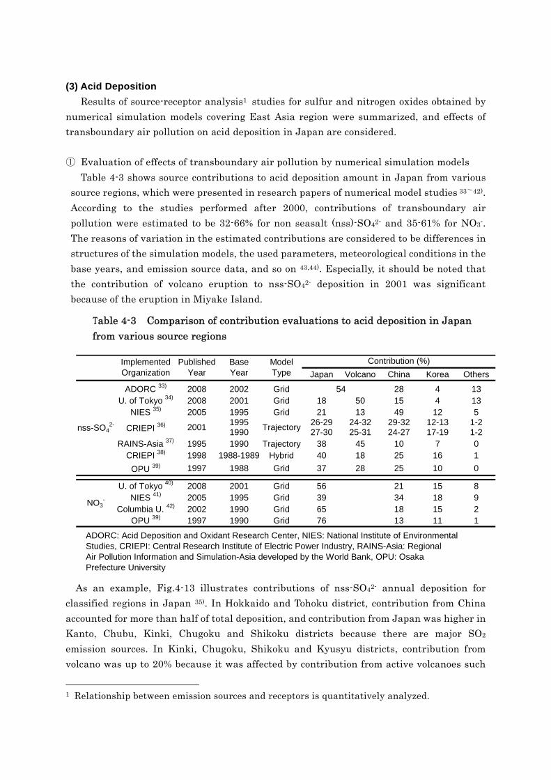
(3) Acid Deposition Results of source-receptor analysis1 studies for sulfur and nitrogen oxides obtained by

numerical simulation models covering East Asia region were summarized, and effects of transboundary air pollution on acid deposition in Japan are considered. ① Evaluation of effects of transboundary air pollution by numerical simulation models

Table 4-3 shows source contributions to acid deposition amount in Japan from various source regions, which were presented in research papers of numerical model studies 33～42). According to the studies performed after 2000, contributions of transboundary air pollution were estimated to be 32-66% for non seasalt (nss)-SO42- and 35-61% for NO3-. The reasons of variation in the estimated contributions are considered to be differences in structures of the simulation models, the used parameters, meteorological conditions in the base years, and emission source data, and so on 43,44). Especially, it should be noted that the contribution of volcano eruption to nss-SO42- deposition in 2001 was significant because of the eruption in Miyake Island.

Japan Volcano China Korea Others

ADORC 33) 2008 2002 Grid 28 4 13U. of Tokyo 34) 2008 2001 Grid 18 50 15 4 13

NIES 35) 2005 1995 Grid 21 13 49 12 51995 26-29 24-32 29-32 12-13 1-21990 27-30 25-31 24-27 17-19 1-2

RAINS-Asia 37) 1995 1990 Trajectory 38 45 10 7 0CRIEPI 38) 1998 1988-1989 Hybrid 40 18 25 16 1

OPU 39) 1997 1988 Grid 37 28 25 10 0

U. of Tokyo 40) 2008 2001 Grid 56 21 15 8NIES 41) 2005 1995 Grid 39 34 18 9

Columbia U. 42) 2002 1990 Grid 65 18 15 2OPU 39) 1997 1990 Grid 76 13 11 1

ADORC: Acid Deposition and Oxidant Research Center, NIES: National Institute of EnvironmentalStudies, CRIEPI: Central Research Institute of Electric Power Industry, RAINS-Asia: RegionalAir Pollution Information and Simulation-Asia developed by the World Bank, OPU: OsakaPrefecture University

Trajectory2001

54

CRIEPI 36)

Contribution (%)

nss-SO42-

ModelType

NO3-

ImplementedOrganization

PublishedYear

BaseYear

As an example, Fig.4-13 illustrates contributions of nss-SO42- annual deposition for classified regions in Japan 35). In Hokkaido and Tohoku district, contribution from China accounted for more than half of total deposition, and contribution from Japan was higher in Kanto, Chubu, Kinki, Chugoku and Shikoku districts because there are major SO2 emission sources. In Kinki, Chugoku, Shikoku and Kyusyu districts, contribution from volcano was up to 20% because it was affected by contribution from active volcanoes such

1 Relationship between emission sources and receptors is quantitatively analyzed.

Table 4-3 Comparison of contribution evaluations to acid deposition in Japan from various source regions

as Mt. Sakurajima. The reason why the contribution from China in the results of Fig.4-13 was higher is not clear at present. When estimated source contributions among different numerical modeling results were compared, the differences in domain of assessment, base year and absolute deposition amounts should be considered.

Table 4-4 shows estimated monthly source contributions of total sulfur deposition in Japan 2002 evaluated by Regional Air Quality Model (RAQM) 33). On the basis of the annual average, contribution of transboundary air pollution accounted for approximately 35% (approximately 30% from China). From the point of view of seasonal variation, no clear variation of contribution from Korea was not seen, whereas contributions from central and southern China were high during autumn and spring and low in summer. The probable reasons of this seasonal trend are that consumption of coal which contains high amounts of sulfur compounds in China is highest in winter and that air pollutants are transported from continent to Japan by prevailing northwestern monsoon in winter.

Jan Feb Mar Apr May Jun Jul Aug Sep Oct Nov Dec Annual Ave.North China 4 5 3 2 2 3 3 3 2 3 4 5 3.3Central China 24 28 21 14 16 13 17 9 9 21 23 17 17.7South China 10 11 10 10 7 8 5 3 3 6 8 6 7.3Korea 3 4 4 5 4 4 5 5 5 5 4 4 4.3Japan 38 36 47 57 64 61 61 73 75 55 38 45 54.2Others 21 16 15 12 7 11 10 7 6 10 22 24 13.4

According to estimated Table 4-4 shows estimated monthly source contributions of total sulfur deposition in Japan 2002 evaluated by Regional Air Quality Model (RAQM) 33). On the basis of the annual average, contribution of transboundary air pollution accounted for approximately 35% (approximately 30% from China). From the point of view of seasonal variation, no clear variation of contribution from Korea was not seen, whereas contributions from central and southern China were high during autumn and spring and low in summer. The probable reasons of this seasonal trend are that consumption of coal

Table 4-4 Estimated monthly source contributions of total sulfur deposition in Japan 2002 (%) 33)

1.15gS/(m 2・year)

0.87gS/(m 2・year)

0.92gS/(m 2・year)

0.82gS/(m 2・year)

1.16gS/(m 2・year)

1.21gS/(m 2・year)

(1.03gS/ (m 2・year))

zone1

zone2

zone3

zone4

zone5

zone6火山

1.15gS/(m 2・year)

0.87gS/(m 2・year)

0.92gS/(m 2・year)

0.82gS/(m 2・year)

1.16gS/(m 2・year)

1.21gS/(m 2・year)

(1.03gS/ (m 2・year))

zone1

zone2

zone3

zone4

zone5

zone6

China

Japan China

Volcano

Total Japan

KoreaTaiwanJapanVolcanoSE AsiaOthers

1.15gS/(m 2・year)

0.87gS/(m 2・year)

0.92gS/(m 2・year)

0.82gS/(m 2・year)

1.16gS/(m 2・year)

1.21gS/(m 2・year)

(1.03gS/ (m 2・year))

zone1

zone2

zone3

zone4

zone5

zone6火山

1.15gS/(m 2・year)

0.87gS/(m 2・year)

0.92gS/(m 2・year)

0.82gS/(m 2・year)

1.16gS/(m 2・year)

1.21gS/(m 2・year)

(1.03gS/ (m 2・year))

zone1

zone2

zone3

zone4

zone5

zone6

China

Japan China

Volcano

Total Japan

KoreaTaiwanJapanVolcanoSE AsiaOthers

Fig.4-13 Estimated contributions of nss-SO42-

annual deposition (gS m-2 yr-1) for classified regions in Japan 1995. 35)

which contains high amounts of sulfur compounds in China is highest in winter and that air pollutants are transported from continent to Japan by prevailing northwestern monsoon in winter.

According to long-term variation of estimated nss-SO42- annual deposition in Japan by using emission amount of SO2 during 1980 and 2000 obtained by REAS (Regional Emission Inventory in Asia, ref. Section 4.2) and Source-receptor matrix calculated for 1995 41), contributions from Japan and China were the comparable level (35%) in 1980. However, the contribution from China increased to 43 % in 1990 and has been 45-50% since 1992 because SO2 emission in China has been increased since the 1980s whereas that in Japan decreased.

According to deposition calculation in Japan from 1995 to 2003 by using the Community Multiscale Air Quality (CMAQ) Modeling System and REAS 45), Fig.4-14 shows the calculated results well agreed with annual and seasonal variations of wet deposition amounts of nss-SO42- (averages at 18 monitoring sites of the Japan Acid Deposition Surveys (JADS)). Furthermore, Fig. 4-15 demonstrates that the deposition amount has rapidly increased since 2000 because of increase in SO2 emission in East Asian region (except the effect of Miyakejima volcano eruption). These results infer that the effect of transboundary air pollution from China is relatively increasing in recent years because SO2 emission in China has been increased whereas that in Japan and Korea decreased.

Meanwhile, contributions of transboundary air pollution to NO3- deposition in Japan were estimated to be different levels, as well as those to SO42- deposition, by various literatures, but it is highly likely that the contribution is increasing with NO3- deposition considering recent trend of NOx emission in Japan and China (ref. Section 4.2) 45).

Mon

thly

nss

-SO

42-w

et d

epos

ition

(nm

olm

-2m

onth

-1)

Observation Values (Averages of 18 sites)Calculated Values (Averages of 18 sites)Calculated Values (National Averages)

Mon

thly

nss

-SO

42-w

et d

epos

ition

(nm

olm

-2m

onth

-1)

Observation Values (Averages of 18 sites)Calculated Values (Averages of 18 sites)Calculated Values (National Averages)

Fig 4-14 Comparison of observed values of nss-SO42- wet deposition amounts (monthly values) and model calculated values 45).

The black solid line indicates the averaged value of 18 JADS monitoring sites, the red dotted line indicates the model calculated average values of 18 JADS monitoring sites, and the blue broken line indicates the model calculated average values of all monitoring sites in Japan.

In summary, model calculation results published after 2000 demonstrated that the recent contribution of transboundary air pollution to acid deposition amounts in Japan is estimated to be approximately 30-65% (approximately 15-50% from China) for nss-SO42- and approximately 35-60% (approximately 20-35% from China) for NO3-. It is considered that the contribution of transboundary air pollution is significant in winter-time northern Japan.

② Evaluation of effects of transboundary air pollution by a sulfur isotope ratio2

It was reported that some researches evaluated effects of transboundary air pollution based on observation data of sulfur isotope ratio (δ34S). δ34S of wet deposition SO42- and nss-SO42- in Niigata prefecture was high in winter and low in summer. This seasonal trend is attributable to higher contribution of sulfur compounds (The contribution to SO42- was estimated to be approximately 20%) emitted from coal combustion origins in northeast Asia region during winter time 47). According to the ditto observation data at 19 Japan nationwide sites in winter, δ34S of nss-SO42- was higher in northern Japan, and the δ34S 2 Since a sulfur isotope ratio of 34S to 32S varies depending on emission origins, the isotope ratio provides information of sulfur cycle in the environment and emission sources of sulfur compounds, δ34S indicates deviation from the isotope ratio of standard material in units of ‰.

Fig 4-15 Estimated variations of nss-SO42- deposition in Japan from 1995 to 2003 45).

The fine broken line indicates the difference of nss-SO42- deposition due to climate change, the bold solid line indicates the difference due to SO2 emissions other than Miyakejima volcano eruption, and the fine dotted line indicates the difference due to SO2 emissions from Miyakejima volcano eruption. The base year for all differences is 2000.

-200

-100

0

100

200

300

1995 1996 1997 1998 1999 2000 2001 2002 2003

年

日本

のnss-SO

42-沈

着量

2000年

との

差　(G

g/年

)

沈着量

気象変化による沈着量の変化

三宅島火山以外の排出量変化による沈着量の変化

三宅島火山の発生量変化による沈着量の変化

Deposition amountChange in deposition due to climate change

Change in deposition due to Miyakejima volcanoChange in deposition due to SO2 emissions

Diff

eren

ce in

nss

-SO

42-de

posi

tion

in J

apan

co

mpa

red

from

that

in 2

000

(Gg/

year

)

Year

value was close to that of coal mined in East Asian countries. This result implies that nss-SO42- wetly deposited in northern Japan was influenced by long range transportation from the Asian continent.

4.3.2 Future prediction of impact of transboundary air pollution on Japan In order to predict impact of transboundary air pollution on Japan, it is important that

atmospheric concentrations of air pollutants are estimated by a chemical transport model and prospected emission amounts of air pollutants, as an input data, on the basis of future trend of socioeconomic activities. Research groups of Frontier Research Center for Global Change, Japan Agency for Marine-Earth Science and Technology (FRCGC/JAMSTEC) and National Institute for Environmental Studies (NIES), etc. promoted future prediction of atmospheric concentrations of air pollutants in East Asia by using the Regional Emission Inventory in Asia (REAS) 3),13) and the Community Multiscale Air Quality (CMAQ) Modeling System 49) as shown in Section 4.2.

Fig. 4-16 shows increase of tropospheric ozone concentration during 2000 and 2020 estimated by 3 kinds of scenarios of REAS and CMAQ 50). The REAS emission inventories employed the following 3 kinds of scenarios for China: Policy Successed Case (PSC), Reference Case (REF) and Policy Failed Case (PFC), and the standard emission scenario on the basis of energy demand prediction by International Energy Agency (IEA) was employed for other countries. It predicted that the annual average of tropospheric ozone concentration in Japan will increase by 0-4 ppbv per year during 2000 and 2020 if the moderate increase emission scenario (REF) was employed. If low emission increase scenario (PSC) was employed, the ozone concentration was estimated to increase by not more than 2 ppbv per year. If high emission increase scenario (PFC) was employed, the ozone concentration was estimated to increase by 2-6 ppbv per year on an annual average and by 2-14 ppbv per year on a monthly average of June when tropospheric ozone concentration becomes higher 50). Especially, ozone concentration in central Honshu was predicted to increase by approximately 6 ppbv on a three month average in summer (June - August) although NOx emission in Japan was predicted to decrease. Since there is no significant difference in emission amounts from other countries except China among different scenarios, future variation of emission from China may largely affect on tropospheric ozone concentration in Japan in the future. Moreover, it should be noted that the emission inventory scenarios of REAS considered 2000 as the base year, and that rapid increased emissions from China after 2000 4),52) were not sufficiently considered. If remarkable economical development in China continues in the future and the PFC scenario become a reality, the tropospheric ozone concentrations in Japan 2020 were predicted to be 45-60 ppbv on an annual average and 50-75 ppbv in June (Fig. 4-16). This prediction raises a concern that ozone pollution in Japan will reach a serious level 53). This prediction also demonstrates emission control such as NOx emission reduction is important to not only environmental protection in China but also countermeasure against photochemical pollution 51).

Medium-term prediction experiments aimed for contribution to the IPCC (Intergovernmental Panel on Climate Change) 4th Assessment Report was carried out by 26 kinds of global chemical transport models. The spate of models employed the 3 kinds of unified emission scenario as follows: Current Legislation (CLE), Maximum Feasible

Fig 4-16 Predicted tropospheric ozone concentration by using 3 kinds of scenarios (PSC, REF and PFC) of REAS 50).

2020PSC-2000: increase in ozone concentration during 2000 and 2020 by using PSC, 2020REF-2000; increase in ozone concentration during 2000 and 2020 by using REF, 2020PFC-2000: increase in ozone concentration during 2000 and 2020 by using PFC, 2020PFC: predicted ozone concentration in 2020 by using PFC.

Reduction (MFR) and IPCC Special Report on Emissions Scenarios A2 (IPCC-A2). When each scenario was incorporated for model simulation, the annual average of surface ozone concentration in East Asia (including Southeast Asia) was estimated to increase by 3.8 ± 0.7 ppbv per year (CLE) and 7.7 ± 1.8 ppbv per year (IPCC-A2) during 2000 and 2030. Only the estimations employed the MFR scenario exhibited decrease in annual ozone concentration (-3.6 ± 0.5 ppbv per year) during the period 54),55). Moreover, these model experiments demonstrated that nitrogen and sulfur deposition amounts were estimated to slightly change (NOy: -3.0 mgNm-2, NHx: +47.0 mgNm-2, SOx: -18.5 mgS m-2) by employing the CLE scenario, largely decrease (NOy: -249.8 mgNm-2, SOx: -404.3 mgS m-2) by the MFR scenario and largely increase (NOy: +278.6 mgNm-2, NHx: +135.0 mgNm-2, SOx: -782.6 mgS m-2) by the IPCC-A2 scenario 56).

It should be noted that these prediction results have large variation among the present global models and the predicted concentrations of air pollutants has larger differences among the different model calculations even if the same emission scenario is employed. Moreover, it should be also noticed that emission amounts in East Asia region will exceed the predicted amounts, and many emission scenarios employed by the above model prediction experiments may not consider this rapid increase of emission amounts. However, these experimental results implies that the atmospheric environment in East Asia region is expected to be in an alarming situation and transboundary air pollution may grow into a more serious problem unless emission regulation will be tightened in the future.

Overview of the model intercomparison study in Asia (MICS-Asia)

Despite the seriousness of transboundary air pollution issues in northern hemisphere, especially, East Asian countries have not built a consensus on common understandings of the issues. In order to build the consensus, numerical simulation by long-range transportation models will play an important role. However, there is significant difference in calculated results among the long-range transportation models targeting on air quality and acid deposition in East Asia developed by researchers in East Asian, American and European countries. Therefore, this discrepancy may be an impediment to the international consensus building. Against this background, the Model Inter-Comparison Study in Asia (MICS-Asia) was launched in 1998, and since 2003, precision comparison of model simulation targeting on SO2, NOx and O3 has been promoted as the MICS-Asia Phase 2 activity.

The MICS-Asia Phase 2 is a joint project between Acid Deposition and Oxidant Research Center and International Institute for Applied Systems Analysis in Austria. Approximately 20 research institutes participate the project, and intercomparisons of long-range transportation models and emission inventories have been promoted. The model calculation results were reported according to the provided data protocol, and finally intercomparison among 8 kinds of models was implemented. The target simulation period was March, July and December in 2002 and March in 2002. This study focused on yellow sand phenomena, high ozone concentration events in Northeast Asia, behaviors of air pollutants in summer and winter. The disclosed EANET (Acid Deposition Monitoring Network in East Asia) monitoring data was used for validation of models.

The projected members summarized the outcomes of the MICS-Asia Phase 2 in 8 research papers that was published in the special issue of “Atmospheric Environment”. The MICS-Asia Phase 3 launched in 2008. The Phase 3 activities will promote analysis of emission contribution in East Asia, comparison with Northern Hemispheric models, analysis of impacts of mega cities in East Asia, relationships between air pollution and climate and development of new emission inventories. References: MICS-Asia Phase 2 Web site (http://www.adorc.gr.jp/adorc/mics.html)

4.4 Intercontinental transport of air pollutants and hemispheric air pollution 4.4.1 Task Force on Hemispheric Transport of Air Pollutants (CLRTAP/TF-HTAP)

Scientific interest of intercontinental transport of air pollution increased in the latter half 1990s, and many research results were presented in the late 1990s 57). At the beginning, the intercontinental transport of yellow sand from the Asian continent to North America via the Pacific Ocean was paid attention 58),59),60),61),62). At that time, in the United States, the possibility that the effect of ozone derived from Asian region was not negligible for achievement of the air quality standards in the Unites States was discussed 63), 64), 65), 66), and, in Europe, the effect of ozone transported from the North America to Europe via the Atlantic Ocean was also discussed 67),68),69),70). The researches focusing on intercontinental transport of ozone from Europe to Asian region via the Eurasian continent demonstrated that effect of North America to Asia was significant as much as that of Europe and ozone originated from Europe and North America considerably impacted on ozone concentration in Asian region 71),72),73). As seen above, it came to light that air pollutants originated from each continent in Northern Hemisphere affected the other continents, and the concept of “hemispheric transport and hemispheric air pollution” was raised.

After the above scientific research outcomes, the Task Force on Hemispheric Transport of Air Pollutants under Convention on Long-range Transboundary Air Pollution (CLRTAP/TF-HTAP) was inaugurated in 2004 at the initiative of the United States and Europe. The secretariat was opened in the United States Environmental Protection Agency (US/EPA) and the United Nations Economic Commission for Europe (UN/ECE). The TF-HTAP is expected to cover technical issues necessary to understand transportation of the air pollutant in the northern hemisphere, and aims to make contributions to the protocol of CLRTAP with a support of a scientific support necessary for policy making. Ozone, aerosol, mercury and Persistent Organic Pollutants (POPs) are designated as target substances for hemispheric transport. The TF-HTAP is composed of experts in the participating countries of the CLRTAP, but it is encouraged to also invite experts in nonmember countries in the Northern Hemisphere. One task force meeting and a set of workshops have been held once a year, and researchers and administrative officers in Japan and other Asian countries have participated in these meetings. In 2006, a workshop on air pollutant emission was held in Beijing, China, which is the first time to be held in a nonmember country. The TF-HTAP prepared the interim assessment report in 2007 and will finalize the report in 2009.

A part of literature review published in the 2007 TF-HTAP interim assessment report is introduced in this section. Table 4-5 summarizes the model calculation results of enhancement of surface ozone in Europe, the United States and Asia as receptor regions affected by North America, Asia and Europe as source regions. For example, the enhancements of surface ozone concentration in Europe affected by North America were reported to be 2-4 ppb on an annual average and 10-15 ppb in some events, and those affected by Asia were 0.8-several ppb on an annual average. The enhancements in the

United States affected by Asia were reported to be 1-4 ppb on an annual average; however, those were 3-10 ppb in some events and up to 30 ppb in the highest event. and 10-15 ppb in some events, and those affected by Asia were 0.8-several ppb on an annual average. The enhancements in Asia affected by Europe and the United States were reported to be 2-3 ppb on an annual average 72),73). In summary, the enhancement of surface ozone concentration in Northern Hemisphere was estimated to be 1-5 ppb on an annual or seasonal average, but the preceding studies commonly pointed out that the enhancement was highest at the end of spring. Since the transport distance across the Atlantic Ocean is shorter than that across the Pacific Ocean or the Eurasian continent, the effect of intercontinental transport from North America to Europe is most significant.

こうした科学的研究成果を受けて 2004 年に米国と EC の主導により長距離越境大気汚染条

約(LRTAP)の下に「大気汚染の半球輸送に関するタスクフォース(TF-HTAP)」が正式に発足し、

US/EPA と UN/ECE とに事務局が置かれた。タスクフォースは、大気汚染物質の北半球輸送

を理解するために必要な技術的問題を扱うとされ、政策立案に必要な科学的サポートを得て、

最終的に条約の議定書に反映させることを目的としている。半球輸送の対象物質としては現在

オゾン、エアロゾルの他に水銀と POPs が扱われている。タスクフォースは条約加盟国の専門

家から構成されているが、北半球の条約非加盟国の専門家を招くことが推奨されている。これ

まで、年に１回のタスクフォース会合と一連のワークショップが開催されており、我が国を初

めとするアジア諸国からも研究者、行政官が参加している。また、大気汚染物質の排出をテー

マにした 2006 年のワークショップは、条約加盟国以外の中国・北京で開催された。TF-HTAPでは 2007 年に中間報告書をとりまとめており、最終報告書を 2009 年にとりまとめることにな

っている。ここではこの中間報告書に取り上げられている文献レビューの一部を紹介する。表 4-5 は地

表オゾンに対しヨーロッパ及び米国を受容(リセプター)領域と見たとき、発生源(ソース)領域で

ある北米、アジア、ヨーロッパからの影響による増加分がどれだけになるかのモデル計算結果

をまとめたものである。例えばヨーロッパに対する北米からの影響は、年平均値では 2-4ppb、イベント的には 10-15ppb、アジアからの影響は年平均で 0.8-数 ppb と報告されている。また、

アジアから米国への影響も年平均では 1-4ppb であるが、イベント的には 3-10ppb、場合によ

っては 30ppb に達するという報告もある。ここにはヨーロッパ、北米からアジアへの影響は掲

げられていないが、それぞれ年平均では 2-3ppb 程度である 73),74)。このように、大陸間輸送の

影響は年平均、季節平均では一般に 1-5ppb 程度であるが、季節的には晩春に最も大きくなる

ことで、これまでの研究の結果は一致している。大西洋をわたる距離が太平洋、ユーラシア大

陸に比べて相対的に短いことから、大陸間輸送は北米からヨーロッパへの影響が最も大きい。

Table 4-5 Estimated enhancements of surface ozone concentration in source regions affected by receptor regions according to existing literatures of intercontinental transport in mid-latitude Northern Hemisphere.

4.4.2 Analysis by intercontinental transportation model As described above, since the late 1990s, some groups have presented the researches on

intercontinental pollutant transport and transformation processes using the seasonal trend data of ozone, carbon monoxide, aerosol and other air pollutants with lifetimes longer than one month. Fig. 4-17 shows characteristics of intercontinental transport of tropospheric ozone via trans-Eurasia (from Europe to Asia), trans-Pacific (from Asia to North America) and trans-Atlantic (from North America to Europe) 72). This figure illustrates how the increased ozone will be transported in a hemispheric scale when emission amounts of anthropogenic NOx, VOC and CO from each continent are increased by 10%. As shown in the left of the figure, ozone generated in Asia is assumed to be transported to the upper troposphere by active vertical convection, which will affect on the hemispherical scale. On the other hand, ozone generated in Europe is assumed to be stay in the middle or lower troposphere because vertical convection is less active, and thus transport to Asia takes place in relatively lower altitude. Ozone generated in North America has the intermediate characteristics between Asia and Europe. These different characteristics are attributable to the difference in latitudes of major polluted areas in each region. The vertical convection in Asia tends to be active because of lower latitude, whereas air mass will stay in the lower troposphere at higher latitude of North America and Europe.

On the basis of the above shown results, effect on ozone and carbon monoxide

concentrations in Happo One, Japan by emissions from North America or Europe is especially shown in Fig. 4-18, depicted as vertical and monthly distributions 73). The enhancement of carbon monoxide affected by Europe was highest in the atmospheric boundary layer during February and March. As is anticipated, the effect of Europe is larger than that of North America On the other hand, the enhancements of ozone affected by both Europe and North America are highest in the middle troposphere during April and May, and the effects of both regions are at the same level. As for surface ozone, the effect of

Increase in emission from Asia

Increase in emissionfrom North America

Increase in emission from Europe

Fig. 4-17 Estimated vertical and planar distributions of ozone concentration when emission amounts of anthropogenic air pollutants from each continent are increased by 10% 72).

Europe is maximum during March and April, and that of North America is during February and March. The enhancements of surface ozone in both regions are at the almost same level (2-3 ppb on a monthly average). The reason why the effect of much farther North America is the same level as that of Europe is that, as shown in Fig. 4-17, ozone generated in North America will be transported into higher altitude than that generated in Europe, which will causes effective long range transport and deposit near Japan.

Fig. 4-19 shows the comparison between the observed surface ozone concentrations at Happo in April 1996, when the effect of intercontinental transport is considered to be relatively significant, and the coetaneous estimated ozone concentrations by a global model, which is the sum of contributed ozone concentrations from each region are shown in the bottom 73). The observed ozone concentration often reached at 60-100 ppb during this period. The contribution from Japan was dominant after April 20, while the contribution of transboundary pollutant transport from East Asian region including China was comparable to that from Japan during April 5-10 and April 15-18. On the other hand, the advections from Europe, North America and the stratosphere significantly contributed to boost background ozone concentration throughout the period. It is a clear

Fig. 4-18 Effects on CO (left) and O3 (right) concentrations in Happo One, Japan by emissions from Europe (upper) and North America (lower), depicted as vertical and monthly distributions 73).

Fig. 4-19 Time profiles of surface O3 (right) concentration in April 1996 at Happo One. The upper shows the observed and calculated concentrations, and the lower shows the contributed ozone concentrations from each region

characteristic that transboundary pollutant transport from East Asian region effects on high ozone concentrations in Japan, which apparently take place some days, and the effect of intercontinental transport has slight daily variation and continuously contributes to background ozone concentration in Japan at a constant level. The contributions from Europe and North America are estimated to be several ppb in total. This amount doesn’t seem to be significant, but it is comparable to transboundary transport from East Asian region on a monthly average basis. This estimation will largely influence on the discussion on adverse effects of ozone on plants, which are generally evaluated by integrated exposed amounts such as AOT40.

References 1) Oden, S., 1976: Water, Air and Soil Pollution, 6, 137-166. 2) Johnson, R.W., G.E. Gordon, Eds., 1987: The Chemistry of Acid Rain, Sources and Atmospheric

Processes, ACS Symposium Series 349, American Chemical Society, Washington, DC 3) EANET, First Periodic Report on the State of Acid Deposition in East Asia, 2007. 4) Ohara, T., Akimoto, H., Kurokawa, J., Horii, H., Yamaji, K., Yan, X., and Hayasaka, T.: An Asian

emission inventory of anthropogenic emission sources for the period 1980-2020, Atmos. Chem. Phys., 7, 4419-4444, 2007.

5) Nakicenovic, N. J. and Swart, R. (Eds.): IPCC special report on emissions scenarios, Cambridge University Press, Cambridge, United Kingdom and New York, NY, 2000.

6) Zhang, Q., Streets, D. G., He, K., Wang, Y., Richter, A., Burrows, J. P., Uno, I., Jang, C. J., Chen, D., Yao, Z., and Lei, Y. : NOx emission trends for China, 1995–2004: The view from the ground and the view from space, J. Geophys. Res., 112, D22306, doi:10.1029/2007JD008684, 2007.

7) Tian, H., Hao, J., and Nie, Y.: Recent trends of NOx emissions from energy use in China, Conference abstracts of Acid Rain 2005, 32, 2005.

8) Hao, J., Tian, H., and Lu, Y.: Emission inventories of NOx from commercial energy consumption in China, 1995–1998, Environ. Sci. Technol., 36, 552–560, 2002.

9) He, Y., Uno, I., Wang, Z., Ohara, T., Sugimoto, N., Shimizu, A., Richter, A., and Burrows, J. P.: Variations of the increasing trend of tropospheric NO2 over central east China during the past decade, Atmos. Environ., 41, 4865-4876, 2007.

10) Streets, D. G., Tsai, N. Y., Akimoto, H., and Oka, K.: Trends in emissions of acidifying species in Asia, 1985–1997, Water Air Soil Poll., 130, 187–192, 2001.

11) Streets, D. G., Bond, T. C., Carmichael, G. R., Fernandes, S. D., Fu, Q., He, D., Klimont, Z., Nelson, S. M., Tsai, N. Y., Wang, M. Q., Woo, J.-H., and Yarber, K. F.: An inventory of gaseous and primary aerosol emissions in Asia in the year 2000, J. Geophys. Res., 108, 8809, doi:10.1029/2002JD003093, 2003.

12) SEPA (State Environmental Protection Administration): Report on the state of the environment in China, State Environmental Protection Administration of China, Beijing, 2003.

13) REAS, http://www.jamstec.go.jp/frcgc/research/p3/emission.htm 14) Byun, DW. and JKS. Ching (Eds.), Science algorithms of the EPA Models-3 community

multi-scale air quality (CMAQ) modeling system, NERL, Research Triangle Park, NC. EPA/600/R-99/030, 1999.

15) Yamaji, K., T. Ohara, I. Uno, H. Tanimoto, J. Kurokawa, and H. Akimoto, Analysis of seasonal variation of ozone in the boundary layer in East Asia using the Community Multi-scale Air Quality model: What controls surface Ozone level over Japan? Atmospheric Environment, 40(10), 1856-1868, 2006.

16) Wild, O., P. Pochanart, and H. Akimoto, Trans-Eurasian transport of ozone and its precursors, Journal of Geophysical Research, 109, D11302, doi:10.1029/2003JD004501, 2004.

17) Sudo, K. and H. Akimoto, Global source attribution of tropospheric ozone: Long-range transport from various source regions, Journal of Geophysical Research, 112, D12302,

doi:10.1029/2006JD007992, 2007. 18) Pochanart, P., S. Kato, T. Katsuno, and H. Akimoto, Eurasian continental background and

regionally polluted levels of ozone and CO observed in northeast Asia, Atmospheric Environment, 38(9), 1325-1336, 2004.

19) Tanimoto, H., Y. Sawa, H. Matsueda, I. Uno, T. Ohara, K. Yamaji, J. Kurokawa, and S. Yonemura, Significant latitudinal gradient in the surface ozone spring maximum over East Asia, Geophysical Research letters, 32, L21805, doi:10.1029/2005GL023514, 2005.

20) Ohara, T., I. Uno, J. Kurokawa, M. Hayasaki, and A. Shimizu, Episodic pollution of photochemical ozone during 8-9 May 2007 over Japan : Overview, J. Jpn. Soc. Atmos. Environ., 43, 198-208, (2008).

21) Takami, A., T. Imai, A. Shimizu, I. Matsui, N. Sugimoto, and S. Hatakeyama, Transport of Anthropogenic and Dust Aerosol Observed at Capr Hedo, Okinawa, J. Aerosol Res., 21, 341-347, (2006).

22) UNECE, Hemispheric Transport of Air Pollution 2007, United Nations, New York, 2007. 23) Uematsu,M., Yoshikawa, A., Muraki, H., Arao, K.,and Uno, I.: Transport of mineral and

anthropogenic aerosols during a kosa event over East Asia, J. Geophys. Res., 107, D7, 4059, doi:10.1029/2001JD000333 (2002).

24) Matsumoto, K., Uyama, Y., Hayano, T., Tanimoto, H., Uno, I. and Uematsu, M.: Chemical properties and outflow patterns of anthropogenic and dust particles on rishiri Island during the Asian Pcific Regional Aerosol Characterization Experiment (ACE-Asia), J. Geophys. Res., 108, D23, 8666, doi:10.1029/2003JD003426 (2003).

25) Igarashi Y., et al., Seasonal variations in SO2 plume transport over Japan: Observations at the summit of Mt. Fuji from winter to summer, Atmos. Environ., 40, 7018-7033 (2006).

26) Uno, I., G. R. Carmichael, D. G. Streets, et al.(2003a): Regional chemical weather forecasting system CFORS: Model descriptions and analysis of surface observations at Japanese island stations during the ACE-Asia experiment, J. Geophys. Res., 108, 8668, doi:10.1029/2002JD002845.

27) Uno, I., G. R. Carmichael, D. Streets, et al.(2003b): Analysis of surface black carbon distributions during ACE-Asia using a regional-scale aerosol model, J. Geophys. Res., 108, 8636, doi: 10.1029/2002JD003252.

28) Jordan, C. E., J. E. Dibb, B. E. Anderson, and H. E. Fuelberg (2003), Uptake of nitrate and sulfate on dust aerosols during TRACE-P, J. Geophys. Res., 108 (D20), 8817, doi:10.1029/2002JD003101.

29) Hatakeyama, S., A. Takami, F. Sakamaki, H. Mukai, N. Sugimoto, A. Shimizu,and H. Bandow, "Aerial measurement of air pollutants and aerosols during March 20–22, 2001, over the East China Sea" J. Geophys. Res., 109, D13304, doi:10.1029/2003JD004271 (2004).

30) Hatakeyama, S., A. Takami, W. Wang, and D. Tang, "Aerial observation of air pollutants and aerosols over Bo Hai, China" Atmos. Environ., 39(32), 5893-5898, doi:10.1016/j.atmosenv.2005.06.025, (2005).

31) Streets, D., T.C. Bond, G.R. Carmichael, S.D. Fernandes, Q. Fu, D. He, Z. Klimont, S.M. Nelson, N.Y. Tsai, M.Q. Wang, J.-H. Woo, and K.F. Yarber (2003), An inventory of gaseous and primary aerosol emissions in Asia in the year 2000, J. Geophys. Res., 108(D21), 8809, doi:10.1029/2002JD003093.

32) Hatakeyama, S., A. Takami, T. Miyoshi, and W. Wang, Relationship among Major Ionic Species in Aerosols Transported from China via the East China Sea to Okinawa, J. Aerosol Res., 21, 147-152 (2006).

33) The secretariat of LTP project, The 11th Expert Meeting for the Long-range Transboundary Air Pollutants in Northeast Asia: Proceeding (2008).

34) Lin, M., T. Oki, M. Bengtsson, S. Kanae, T. Holloway, D.G. Streets (2008). Long-range transport of acidifying substances in East Asia—Part II:Source-receptor relationships. Atmospheric Environment, 42, 5956-5967.

35) Inoue, M., T. Ohara, M. Katayama, and K. Murano, Annual Source-receptor Relationships of Sulfur in East Asia Using a Numerical Simulation Model RAMS/HYPACT, J. Aerosol Res., 20, 333-344 (2005).

36) Ichikawa, Y., H. Hayami, T. Sugiyama, M. Amann, and W. Schopp (2001). Forecast sulfur deposition in Japan for various energy supply and emission control scenarios, Water, Air, & Soil Pollution, 130, 301-306.

37) Carmichael G. R. and R. L. Arndt (1995) Chapter 5, ATMOS module, Long range transport and deposition of sulfur in Asia (Rains-Asia: An assessment model for air pollution in Asia, Foell, W. et al., Report on the World Bank Sponsored Project “Acid Rain and Emission Reductions in Asia”), V51-V58.

38) Ichikawa, Y., H. Hayami, and S. Fujita (1998) A long-range transport model for East Asia to estimate sulfur deposition in Japan, J. Applied Meteorology, 37, 1364-1374.

39) Ikeda Y. and H. Higashino, The Estimation of Acid Deposition in East Asia (II) : Focused on the Ratio of Sources Contribution of the Deposition, J. Jpn. Soc. Atmos. Environ., 32, 175-186 (1997).

40) Lin, M., T. Oki, T. Holloway, D.G. Streets, M. Bengtsson, S. Kanae (2008). Long-range transport of acidifying substances in East Asia—Part I:model evaluation and sensitivity studies. Atmospheric Environment, 42, 5939-5955.

41) Ohara, T., M. Inoue, M. Katayama, and K. Murano (2005). Annual source-receptor relationships of sulfur and nitrogen oxides in East Asia using a regional transport modeling system coupled with a meteorological model, Conference abstracts of Acid Rain 2005, 57.

42) Holloway, T., H. Levy II, and G. Carmichael (2002). Transfer of reactive nitrogen in Asia: development and evaluation of a source-receptor model, Atmos. Environ., 36, 4251-4264.

43) Carmichael, G., et al. (2001). Model intercomparison study of long range transport and sulfur deposition in East Asia (MICS-ASIA), Water, Air, & Soil Pollution, 130, 51-62.

44) Acid Deposition Monitoring Network in East Asia (EANET), Periodic report on the state of acid deposition in East Asia, Part 1: Regional Assessment, 2006.

45) Katayama, M., T. Ohara, I. Uno, and H. Hara, Model Analysis of Inter-annual Variations of Sulfur Deposition in Japan, J. Jpn. Soc. Atmos. Environ., 43, 136-146 (2008).

46) Uno, I., M. Uematsu, Y. Hara, Y. J. He, T. Ohara, A. Mori, T. Kamaya, K. Murano,Y. Sadanaga, and H. Bandow (2007). Numerical study of the atmospheric input of anthropogenic total nitrate to the marginal seas in the western North Pacific region, Geophys. Res. Lett., 34, L17817, doi:10.1029/2007GL030338.

47) Ohizumi, T., N. Fukuzaki, and M. Kusakabe (1997). Sulfur isotopic view on the sources of sulfur

in atmospheric fallout along the coast of the sea of Japan, Atmos. Environ., 31, 1339-1348. 48) Yanagisawa, F., N. Akata, R. Motoyama, A. Kawabata, and A. Ueda (2001). Seasonal variation of

sulfur isotope ratios on non-sea salt sulfate in wet deposition in Japan, J. Ecotechnology Res., 7, 1-6.

49) Byun, D.W. and J.K.S. Ching (Eds.), Science algorithms of the EPA Models–3 community multiscale air quality (CMAQ) modeling system. NERL, Research Triangle Park, NC. EPA/600/R-99/030, 1999.

50) Yamaji, K., Ohara, T., Uno, I., Kurokawa, J., Pochanart, P., and Akimoto H., Future Prediction of Surface Ozone over East Asia using Models–3 Community Multiscale Air Quality Modeling System (CMAQ) and Regional Emission Inventory in ASia (REAS), JGR-Atmosphere, Accepted.

51) Press release of the Japan Agency for Marine-Earth Science and Technology, “Projection of Future Ozone Concentration Using Air Pollution Emission Scenario in Asia”, (April 24, 2008).

52) Akimoto, H., T. Ohara, J.Kurokawa, and N. Horii, Verification of energy consumption in China during 1996–2003 by satellite observation, Atmos. Environ., 40, 7663–7667, 2006

53) Yamaji, K., and H. Akimoto, The status quo and future prediction of East Asian ozone pollution learned from recent model studies, J. Resour. Environ., 43(7), 28-35, (2007).

54) Stevenson, D.S., F.J. Dentener, M.G. Schultz, K. Ellingsen, T.P.C. van Noije, O. Wild, G. Zeng, M. Amann, C.S. Atherton, N. Bell, D.J. Bergmann, I. Bey, T. Butler, J. Cofala, W.J. Collins, R.G. Derwent, R.M. Doherty, J. Drevet, H.J. Eskes, A.M. Fiore, M. Gauss, D.A. Hauglustaine, L.W. Horowitz, I.S.A. Isaksen, M.C. Krol, J.-F. Lamarque, M.G. Lawrence, V. Montanaro, J.-F. Müller, G. Pitari, M.J. Prather, J.A. Pyle, S. Rast, J.M. Rodriguez, M.G. Sanderson, N.H. Savage, D.T. Shindell, S.E. Strahan, K. Sudo, and S. Szopa, Multimodel ensemble simulations of present–day and near-future tropospheric ozone, JGR-Atmosphere, 2006.

55) Dentener, F., D. Stevenson, K. Ellingsen, T. van Noije, M. Schultz, M. Amann, C. Atherton, N. Bell, D. Bergmann, I. Bey, L. Bouwman, T. Butler, J. Cofala, B. Collins, J. Drevet, R. Doherty, B. Eickhout, H. Eskes, A. Fiore, M. Gauss, D. Hauglustaine, L. Horowitz, I. Isaksen, B. Josse, M. Lawrence, M. Krol, J.F. Lamarque, V. Montanaro, J.F. Muller, V.H. Peuch, G. Pitari, J. Pyle, S. Rast, J. Rodriguez, M. Sanderson, N.H. Savage, D. Shindell, S. Strahan, S. Szopa, K. Sudo, R. Van Dingenen, O. Wild, G. Zeng, The global atmospheric environment for the next generation, EST, 40(11), 3586–3594, 2006.

56) Dentener, F., J. Drevet, J. F. Lamarque, I. Bey, B. Eickhout, A. M. Fiore, D. Hauglustaine, L. W. Horowitz, M. Krol, U. C. Kulshrestha, M. Lawrence, C. Galy-Lacaux, S. Rast, D. Shindell, D. Stevenson, T. Van Noije, C. Atherton, N. Bell, D. Bergman, T. Butler, J. Cofala, B. Collins, R. Doherty, K. Ellingsen, J. Galloway, M. Gauss, V. Montanaro, J. F. Mu¨ ller, G. Pitari, J. Rodriguez, M. Sanderson, F. Solmon, S. Strahan, M. Schultz, K. Sudo, S. Szopa, and O. Wild, Nitrogen and sulfur deposition on regional and global scales: A multimodel evaluation, GBC, 20, GB4003, doi:10.1029/2005GB002672,2006.

57) Akimoto, H., Intercontinental Transport of Air Pollutants and Hemispheric Air Pollution, J. Jpn. Soc. Atmos. Environ, 41(1), A1-A8, (2006).

58) Husar, R.B., et al. (2001) The Asian dust events of April 1998, J. Geophys. Res., 106, 18, 18317-18333.

59) Jaffe, D., T. Anderson, D. Convert, K. Kotchenruther, B. Trost, J. Daneilson, W. Simpson, Bernstein, T.K., S. Karlsdottir, D. Blake, J. Harris, G. Carmichael (1999) I. Uno, Transport of Asian air pollution to North America, Geophys. Res. Lett., 26, 711-714.

60) McKendry, I.G., J.P. Hacker, R. Stull, S. Sakiyam, D. Mignacca, and K. Reid (2001) Long-range transport of Asian dust to the Lower Fraser Valley, British Columbia, Canada, J. Geophys. Res., 106, 18,361-18,370.

61) Uno, I., H. Amano, S. Emori, K. Kinoshita, I. Matsui, , NN. Sugimoto (2001) Trans-Pacific yellow sand transport observed in April 1998: A numerical simulation, J. Geophys. Res., 106, 18331-18344.

62) Vaughan, J.K., C. Claiborn, and D. Finn (2001) April 1998 Asian dust event over the Columbia Plateau, J. Geophys. Res., 106, 18,381-18,402.

63) Bernstein, T.K., S. Karlsdottir, D.A. Jaffe (1999) Influence of Asian emissions on the composition of air reaching the north eastern United States, Geophys. Res. Lett., 26, 2171-2174.

64) Jacob D.L., J.A. Logan, P.P. Murti (1999) Effect of rising Asian emissions on surface ozone in the United States, Geophys. Res. Lett., 26, 2175-2178.

65) Yienger, J. J., M. Galanter, T. A. Holloway, M. J. Phadnis, S. K. Guttikunda, G. R. Carmichael, W. J. Moxim, and H. Levy II (2000) The Episodic Nature of Air Pollution Transport from Asia to North America. J. Geophys. Res., 105, 26,931-26,945.

66) Fiore, A.M., D.J. Jacob, I. Bey, R.M. Yantosca, B.D. Field, A.C. Fusco, and J.G. Wilkinson (2002) Background ozone over the United States in summer: Origin,trend, and contribution to pollution episodes, J. Geophys. Res., 107 (D15), doi:10.1029/2001JD000982.

67) Derwent, R.G., P.G. Simmonds, S. Seuring, C. Dimmer (1998) Observation and interpretation the seasonal cycles in the surface concentrations of ozone and carbon monoxide at Mace Head, Ireland from 1990 to 1994, Atmos. Environ., 32, 145-157.

68) Li, Q., D. J. Jacob, I. Bey, P.I. Palmer, B.N. Duncan, et al. (2002) Transatlantic transport of pollution and its effects on surface ozone in Europe and North America, J. Geophys., Res., 107, dio:10.1029/2001JD001422.

69) Stohl, A., and Trickl (1999) A textbook example of long-range transport: Simultaneous observations of ozone maxima of stratospheric and North American origin in the free troposphere over Europe, J. Geophys. Res., 104, 30,445-30,462.

70) Stohl, A., S. Eckhart, C. Forster, P. James (2002) Spichtinger, J. Geophys. Res., 106, doi.:1029/2001 JD001396.

71) Pochanart, P., H. Akimoto, Y. Kajii, V.M. Potemkin, and T. Khodzer (2003) Regional background ozone and carbon monoxide variations in remote Siberia/ East Asia, J. Geophys. Res., 108, doi: 10.1029/2001JD001412

72) Wild O., and H. Akimoto (2001) Intercontinental transport of ozone and its precursors in a three dimensional global CTM, J. Geophys. Res., 106, 27,729-27,744.

73) Wild, O, and H. Akimoto (2004) Trans-Eurasian transport of ozone and its precursors, J. Geophys. Res., 109, doi:10.1029/2003JD004501.