REPORT

On

Adaptive Filters- Implementation and

Applications

BY:

ADITYA MANGLIK 2014A3PS296P

RISHABH BHARDWAJ 2014A3PS179P

AT

BIRLA INSTITUTE OF TECHNOLOGY & SCIENCE, PILANI

A Digital Signal Processing Report

BIRLA INSTITUTE OF TECHNOLOGY & SCIENCE,

PILANI

19th November, 2016

ACKNOWLEGMENTS

We would like to thank Dr. Pawan K. Ajmera for giving us the

opportunity to pursue this project. It was a wonderful learning

opportunity that helped us expand our knowledge in the domain of

Digital Signal Processing. We are also grateful to the lab

assistants/TAs of this course for their collaboration and helping us

throughout this journey. Without this team, we would have never

learned as much as we did.

ABSTRACT

The goal of this report is to review existing literature on different kinds of

adaptive filters used in Digital Signal Processing today. We have

discussed about the benefits of using adaptive filters over simple finite

impulse response (FIR) filters. The paper also discusses algorithms and

order of complexity for each algorithm so as to gain more insights about

the filtering operation. After the whole literature review, we have

discussed and implemented adaptive noise filtering implementations for

LMS, XLMS, NLMS, RLS and Affine Projection.

The report also includes the graphical interface designed in MATLAB to

get a graphical view of filtering operation done by different techniques.

INTRODUCTION

In the case of Linear Filter, the filter output is a linear function of the

filter input. Design methods available are the classical approach based

methods such as frequency-selective filters (Low-Pass/ Band-Pass/ High-

Pass/ Notch Filters etc.). The second is optimal filter design based mostly

on minimizing the mean-square value of the error signal. Weiner

proposed a filter in 1942(Weiner filter) which was based on priori

statistical information. When such a priori information is not available

(which is the case usually); it is not possible to design a Weiner filter in

the first place. The signal and/or noise characteristics are often non-

stationary and the statistical parameters vary with time. An adaptive filter

has an adaptation algorithm that is meant to monitor the environment and

vary the filter transfer function accordingly. Hence, based in the actual

signals received, the adaptive filter attempts to find the optimal filter

design. The basic operation now involves two processes:

a) Filtering process, which produces the output signal in response to a

given input signal.

b) Adaptive process, which aims to adjust the filter parameters (filter

transfer function) to the (possibly time-varying) environment.

Often, the (average) square value of the error signal is used as the

optimization criterion. The aim is to adapt the digital filter such that the

input signal is filtered to produce output which when subtracted from

desired signal, will minimize the power of the error signal. Hence,

adaptive filters are also called as self-learning filters, whereby an FIR (or

IIR) is designed based on the characteristics of the input signals.

2. ADAPTIVE FILTER

An adaptive filter is a device dedicated to model the relationship between

two signals in real time in a computationally iterative manner. Adaptive

filters are often realized either as a set of program instructions running on

a processing device such as a specific Digital Signal Processing

chip(ASIC), or as a set of logic operations implemented in a field-

programmable gate array (FPGA).

For this project, we shall focus on the mathematical forms of adaptive

filters as opposed to their specific realizations in software or hardware.

An adaptive filter is defined by four aspects:

1. The signal being processed by the filter.

2. The structure that defines how the output signal of the filter is

computed from its input signal.

3. The parameters within this structure that can be iteratively changed

to alter the filter’s input-output relationship.

4. The adaptive algorithm that describes how the parameters are

adjusted from one time instant to the next.

One of the problems that arises in several applications is the identification

of a system or, equivalently, finding its input-output response

relationship. To succeed in determining the filter coefficients that

represent a model of the unknown system, we set a system configuration

according to the diagram shown in Figure 1.1.

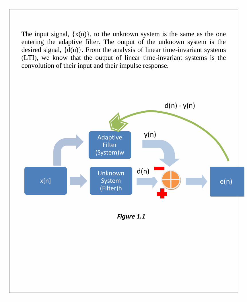
The input signal, {x(n)}, to the unknown system is the same as the one

entering the adaptive filter. The output of the unknown system is the

desired signal, {d(n)}. From the analysis of linear time-invariant systems

(LTI), we know that the output of linear time-invariant systems is the

convolution of their input and their impulse response.

x[n]Unknown

System (Filter)h

Adaptive Filter

(System)w

e(n)

Figure 1.1

d(n)

y(n)

d(n) - y(n)

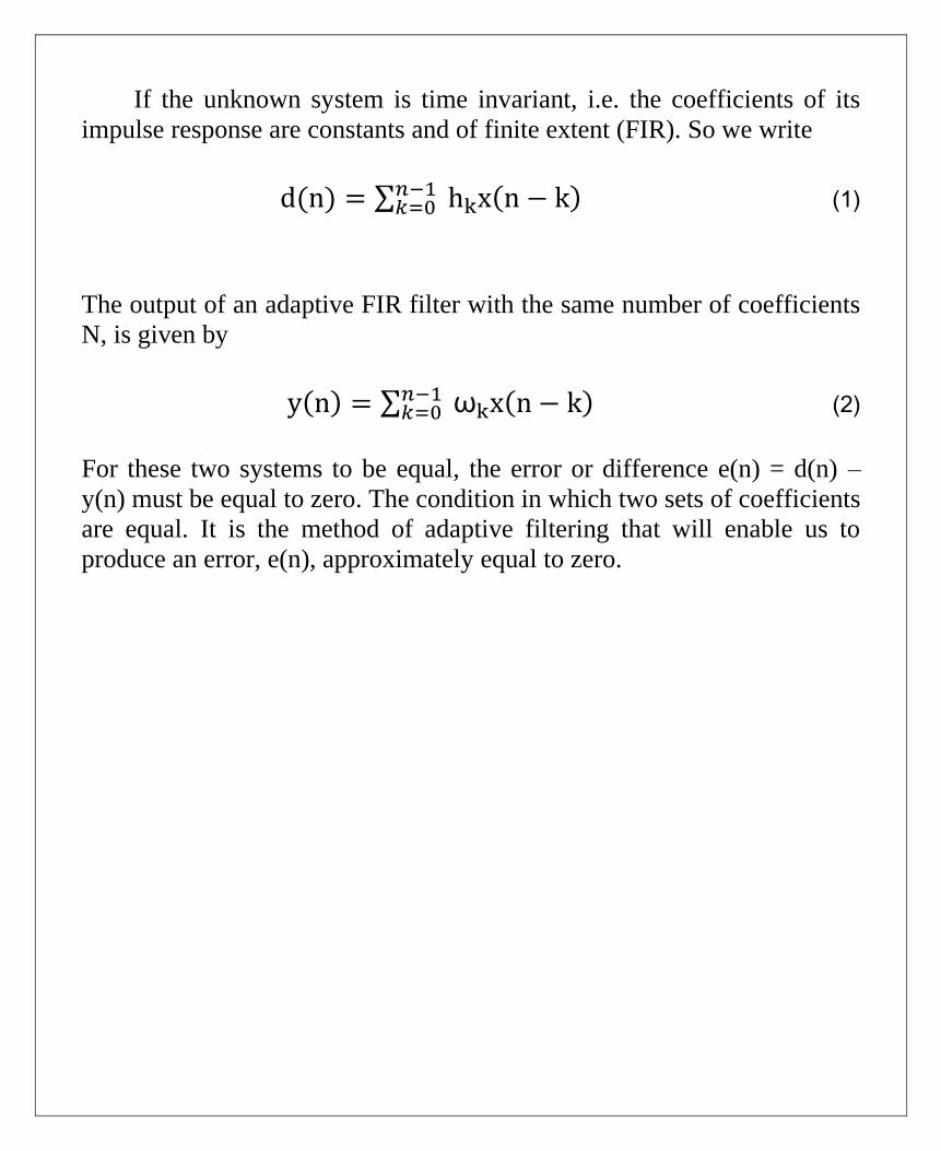
If the unknown system is time invariant, i.e. the coefficients of its

impulse response are constants and of finite extent (FIR). So we write

d(n) = ∑ hkx(n − k)𝑛−1𝑘=0 (1)

The output of an adaptive FIR filter with the same number of coefficients

N, is given by

y(n) = ∑ ωkx(n − k)𝑛−1𝑘=0 (2)

For these two systems to be equal, the error or difference e(n) = d(n) –

y(n) must be equal to zero. The condition in which two sets of coefficients

are equal. It is the method of adaptive filtering that will enable us to

produce an error, e(n), approximately equal to zero.

2.1. Filtering Random Process

A discrete random signal {X(n)} is a sequence of indexed random

variable assuming the values:

{x(0),x(1),x(2),…}

This is also called a time series if the random variable is continuous at any

time.

Stationary process is a time sequence in which joint probability

distribution does not change when shifted in time. A special kind of

random signal is White noise, a random process of uncorrelated random

variables, or WGN.

Linear time-invariant filters are used in many signal processing

applications. Since the input signals of these filters are usually random

process, we need to determine how the statistic of these signals is

modified as a result of filtering.

A wide sense stationary (WSS) process {x(n)} may be realized as the

output of a causal and stable filter h(n) that is driven by white noise v(n)

having variance 𝜎2 . This process is known as the innovation process.

2.2. Special Types of Random Process

Autoregressive moving average process (ARMA)

A shift-invariant stable system with p poles and q zeros can be

represented in the general form

𝐻(z) =𝐵(𝑧)

𝐴(𝑧)

∑ b(k)z−k𝑞

𝑘=0

1+∑ b(k)z−k𝑝

𝑘=0

(3)

If a white noise, v(n), with variance 𝜎𝑣

2 is the input to the above filter,

the output process x(n) is a WSS process and its power spectrum is given

by

𝑆𝑥(𝑧) = 𝜎𝑣2 𝐵(𝑧)𝐵(𝑧−1)

𝐴(𝑧)𝐴(𝑍−1) (4)

The process having above power spectral density is known as the

autoregressive moving average process of order (p,q).

(5)

A special and important type of ARMA process results when set q=0

called Autoregressive process (AR).

2.3. LMS (Least Mean Squares) Algorithm

Most popular adaptation algorithm is LMS. Define cost function as mean

– square error. The algorithm is based on the method of steepest descent

method. Moving towards the minimum on the error surface to get to

minimum gradient of the error surface estimated at every iteration.

Updated old value of learning tap- error

Value of = tap – weight + rate x input x signal

Tap- weight vector Parameter vector

Vector

(8) Simple, no matrices calculation involved in the adaptation and in the

family of stochastic gradient algorithms. The algorithm is based in

the minimum mean square criterion (MMSE). Adaptive process

containing two input signals: a) Filtering process, producing output

signal. b) Desired signal (Training sequence).

1) The filter output is given by :

(7)

2) Estimation error :

e(n) = d(n) – y(n) (8)

3) Tap-weight adaptation:

(9)

1

0

*M

k

k nwknuny

neknunwnw kk

*1

2.3.1. Noise Cancellation:

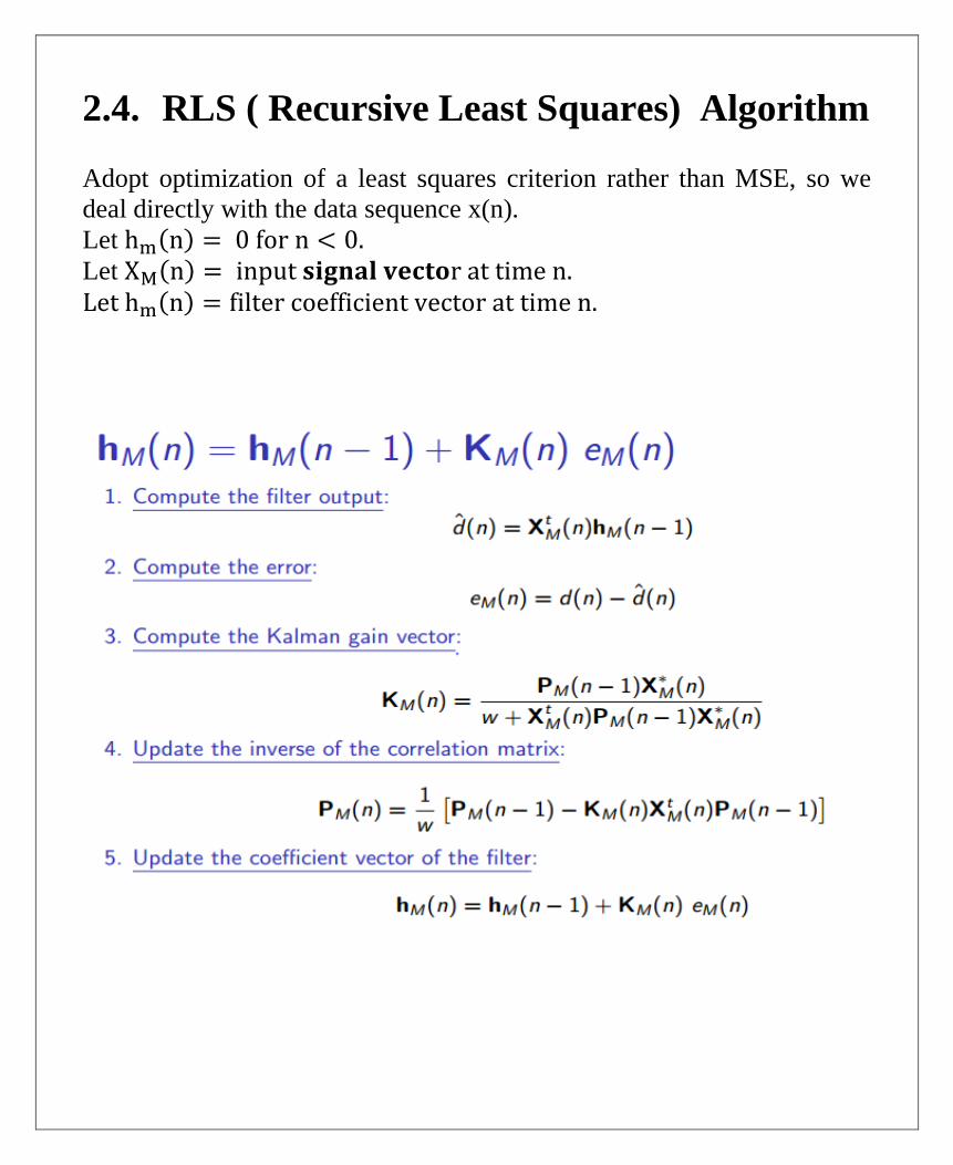
2.4. RLS ( Recursive Least Squares) Algorithm Adopt optimization of a least squares criterion rather than MSE, so we

deal directly with the data sequence x(n).

Let hm(n) = 0 for n < 0. Let XM(n) = input 𝐬𝐢𝐠𝐧𝐚𝐥 𝐯𝐞𝐜𝐭𝐨r at time n. Let hm(n) = filter coefficient vector at time n.

2.4.1. Noise Cancellation:

3. NLMS (Normalized Least Mean Squares)

Algorithm

The main drawback of the simple LMS algorithm is that it is

sensitive to the scaling of its input. This makes it very hard to

choose a learning rate µ that guarantees stability of the algorithm.

The Normalized least mean squares (NLMS) filter is a variant of the

LMS algorithm. The benefit is that it solves this problem by

normalizing with the power of the input.

3.1. Noise Cancellation:

4. Comparison between different algorithms

RLS has rapid rate of convergence compared to LMS.

LMS is computationally simply than RLS.

LMS is sensitive to scaling of its input. So, NLMS comes into the

picture to solve the problem.

RLS algorithms are known for their excellent performance when

working in time varying environments but at the cost of an

increased computational complexity and some stability problems.

High Low Low

In the RLS Algorithm the estimate of previous samples of output

signal, error signal and filter weight is required that leads to

higher memory requirements.

It is clear from the graphs, LMS algorithm takes more iteration

required for achieve the steady state error (ess) but in NLMS and

RLS algorithm to achieve the steady state error is less number of

iteration along with mean square error is also less as compared to

LMS algorithm for different weight vector.

References

[1] Adaptive Filtering by Thomas Spring 1998. [2] Adaptive Filtering Algorithms for Noise Cancellation by Rafel Merredin Alves Falcao. [3] Haykin, S., “Adaptive filter theory”, 3rd Edition, Prentice Hall, 1996 [4] B. Farhang-Boroujeny, “Adaptive Filters: Theory and Applications”, Wiley, 1998 [5] Gale, Z., “GMC Terrain Crossover uses Noise Cancelling Tech to Quiet Cabin, Help Efficiency”, Truck Trend Magazine, February 25, 2011 [6] Diniz, P. S. R., “Adaptive Filtering – Algorithams and Practical Implementation”, Thrird Edition, Kluwer Academic Publishers, 2008 [7] Sayed, A.H., “Fundamentals of Adaptive Filtering”, John Wiley & Sons, New Jersey, 2003 [8] Górriz, J.M.; Ramírez, J.; Cruces-Alvarez, S.; Puntonet, C.G.; Lang, E.W.; Erdogmus, D., “A Novel LMS Algorithm Applied to Adaptive Noise Cancellation”, IEEE Signal Processing Letters, VOL. 16, NO. 1, January 2009

Appendix

The code for the GUI is given below:

function varargout = DSP(varargin) % Begin initialization code - DO NOT EDIT gui_Singleton = 1; gui_State = struct('gui_Name', mfilename, ... 'gui_Singleton', gui_Singleton, ... 'gui_OpeningFcn', @DSP_OpeningFcn, ... 'gui_OutputFcn', @DSP_OutputFcn, ... 'gui_LayoutFcn', [] , ... 'gui_Callback', []); if nargin && ischar(varargin{1}) gui_State.gui_Callback = str2func(varargin{1}); end

if nargout [varargout{1:nargout}] = gui_mainfcn(gui_State, varargin{:}); else gui_mainfcn(gui_State, varargin{:}); end % End initialization code - DO NOT EDIT

% --- Executes just before DSP is made visible. function DSP_OpeningFcn(hObject, eventdata, handles, varargin) % This function has no output args, see OutputFcn. % hObject handle to figure % eventdata reserved - to be defined in a future version of MATLAB % handles structure with handles and user data (see GUIDATA) % varargin command line arguments to DSP (see VARARGIN)

% Choose default command line output for DSP handles.output=hObject; % Update handles structure guidata(hObject, handles);

% UIWAIT makes DSP wait for user response (see UIRESUME) % uiwait(handles.figure1);

% --- Outputs from this function are returned to the command line. function varargout = DSP_OutputFcn(hObject, eventdata, handles) % varargout cell array for returning output args (see VARARGOUT); % hObject handle to figure % eventdata reserved - to be defined in a future version of MATLAB % handles structure with handles and user data (see GUIDATA)

% Get default command line output from handles structure varargout{1} = handles.output;

%% Order text input function edit2_Callback(hObject, eventdata, handles) % hObject handle to edit2 (see GCBO) % eventdata reserved - to be defined in a future version of MATLAB % handles structure with handles and user data (see GUIDATA)

% Hints: get(hObject,'String') returns contents of edit2 as text % str2double(get(hObject,'String')) returns contents of edit2 as a double handles.order=str2double(get(hObject,'String')); % Update handles structure guidata(hObject, handles);

%% Step Size text input function edit3_Callback(hObject, eventdata, handles) % hObject handle to edit3 (see GCBO) % eventdata reserved - to be defined in a future version of MATLAB % handles structure with handles and user data (see GUIDATA)

% Hints: get(hObject,'String') returns contents of edit3 as text % str2double(get(hObject,'String')) returns contents of edit3 as a double handles.mu=str2double(get(hObject,'String')); % Update handles structure guidata(hObject, handles);

%% Input Signal Menu- Executes on selection change in popupmenu2. function popupmenu2_Callback(hObject, eventdata, handles) % hObject handle to popupmenu2 (see GCBO) % eventdata reserved - to be defined in a future version of MATLAB % handles structure with handles and user data (see GUIDATA)

% Hints: contents = cellstr(get(hObject,'String')) returns popupmenu2 contents as

cell array % contents{get(hObject,'Value')} returns selected item from popupmenu2 val = get(hObject,'Value');

switch val case 1 %User selects Data File [FileName,~] = uigetfile('*.txt','Select the data file'); handles.input_type=1; data=importdata(FileName); handles.input_data=data;

case 2 %User selects Audio File [FileName,~] = uigetfile('*.wav','Select the audio file'); handles.input_type=2; [data,handles.Fs]=audioread(FileName); handles.input_data=data;

case 3 %User selects Data File [FileName,~] = uigetfile('*.jpg','Select the image file'); handles.input_type=3; %Add function to import image file data=importdata(FileName); handles.input_data=data; end axes(handles.axes1) plot(abs(fft(handles.input_data))); xlabel('Frequency(Hz)'); ylabel('Magnitude');

% Update handles structure guidata(hObject, handles);

%% Output Display menu --- Executes on selection change in popupmenu3. function popupmenu3_Callback(hObject, eventdata, handles) % hObject handle to popupmenu3 (see GCBO) % eventdata reserved - to be defined in a future version of MATLAB

% handles structure with handles and user data (see GUIDATA)

% Hints: contents = cellstr(get(hObject,'String')) returns popupmenu3 contents as

cell array % contents{get(hObject,'Value')} returns selected item from popupmenu3 val = get(hObject,'Value'); axes(handles.axes4) switch val case 1 %User selects Frequency Response handles.output_type=1; hold on plot(abs(fft(handles.input_data)),'r'); plot(abs(fft(handles.output_data)),'b'); xlabel('Frequency(Hz)'); ylabel('Magnitude'); hold off case 2 %User selects Filter Coeffs handles.output_type=2; figure

end % Update handles structure guidata(hObject, handles);

%% FILTER Menu--- Executes on selection change in popupmenu1 function popupmenu1_Callback(hObject, eventdata, handles) % hObject handle to popupmenu1 (see GCBO) % eventdata reserved - to be defined in a future version of MATLAB % handles structure with handles and user data (see GUIDATA)

% Hints: contents = cellstr(get(hObject,'String')) returns popupmenu1 contents as

cell array % contents{get(hObject,'Value')} returns selected item from popupmenu1 val=get(hObject,'value');

switch val case 1 handles.filter_type=1; case 2 handles.filter_type=2; case 3 handles.filter_type=3; case 4 handles.filter_type=4; case 5 handles.filter_type=5; end % Update handles structure guidata(hObject, handles);

%% Filter Button --- Executes on button press in pushbutton6. function pushbutton6_Callback(hObject, eventdata, handles) % hObject handle to pushbutton5 (see GCBO) % eventdata reserved - to be defined in a future version of MATLAB % handles structure with handles and user data (see GUIDATA)

switch handles.filter_type case 1 %LMS

handles.output_data=DSPFilterLMS(handles.desired_data,handles.input_data,handles.order,ha

ndles.mu); case 2 %NLMS

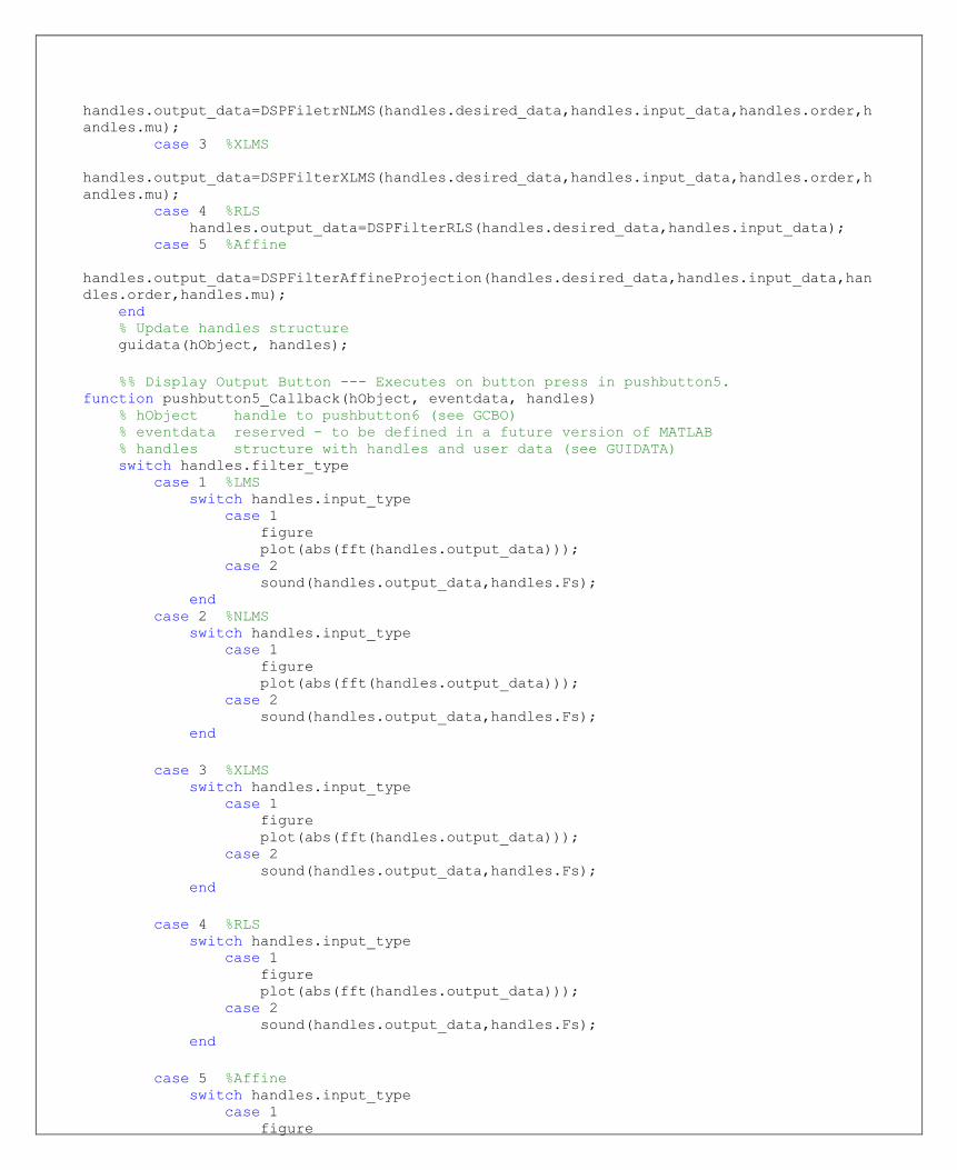
handles.output_data=DSPFiletrNLMS(handles.desired_data,handles.input_data,handles.order,h

andles.mu); case 3 %XLMS

handles.output_data=DSPFilterXLMS(handles.desired_data,handles.input_data,handles.order,h

andles.mu); case 4 %RLS handles.output_data=DSPFilterRLS(handles.desired_data,handles.input_data); case 5 %Affine

handles.output_data=DSPFilterAffineProjection(handles.desired_data,handles.input_data,han

dles.order,handles.mu); end % Update handles structure guidata(hObject, handles);

%% Display Output Button --- Executes on button press in pushbutton5. function pushbutton5_Callback(hObject, eventdata, handles) % hObject handle to pushbutton6 (see GCBO) % eventdata reserved - to be defined in a future version of MATLAB % handles structure with handles and user data (see GUIDATA) switch handles.filter_type case 1 %LMS switch handles.input_type case 1 figure plot(abs(fft(handles.output_data))); case 2 sound(handles.output_data,handles.Fs); end case 2 %NLMS switch handles.input_type case 1 figure plot(abs(fft(handles.output_data))); case 2 sound(handles.output_data,handles.Fs); end

case 3 %XLMS switch handles.input_type case 1 figure plot(abs(fft(handles.output_data))); case 2 sound(handles.output_data,handles.Fs); end

case 4 %RLS switch handles.input_type case 1 figure plot(abs(fft(handles.output_data))); case 2 sound(handles.output_data,handles.Fs); end

case 5 %Affine switch handles.input_type case 1 figure

plot(abs(fft(handles.output_data))); case 2 sound(handles.output_data,handles.Fs); end

end % Update handles structure guidata(hObject, handles);

%% Input Signal Button --- Executes on button press in pushbutton1. function pushbutton1_Callback(hObject, eventdata, handles) % hObject handle to pushbutton1 (see GCBO) % eventdata reserved - to be defined in a future version of MATLAB % handles structure with handles and user data (see GUIDATA)

switch handles.input_type case 1 %User selects Data File msgbox('Input signal is plotted in Axis 1'); case 2 %User selects Audio File sound(handles.input_data,handles.Fs);

case 3 %User selects Image File %Add function to display image file end % Update handles structure guidata(hObject, handles); %% Desired Signal Button--- Executes on button press in pushbutton7. function pushbutton7_Callback(hObject, eventdata, handles) % hObject handle to pushbutton7 (see GCBO) % eventdata reserved - to be defined in a future version of MATLAB % handles structure with handles and user data (see GUIDATA) switch handles.input_type case 1 %User selects Data File [FileName,~] = uigetfile('*.txt','Select the data file'); data=importdata(FileName); handles.desired_data=data;

case 2 %User selects Audio File [FileName,~] = uigetfile('*.wav','Select the audio file'); [data,handles.Fs]=audioread(FileName); handles.desired_data=data; %x=numel(abs(fft(handles.desired_data)));

case 3 %User selects Data File [FileName,~] = uigetfile('*.jpg','Select the image file'); %Add function to import image file data=importdata(FileName); handles.desired_data=data; end axes(handles.axes4) plot(abs(fft(handles.desired_data)),'r'); xlabel('Frequency(Hz)'); ylabel('Magnitude'); % Update handles structure guidata(hObject, handles);

%% Display Desired Button --- Executes on button press in pushbutton8. function pushbutton8_Callback(hObject, eventdata, handles) % hObject handle to pushbutton1 (see GCBO) % eventdata reserved - to be defined in a future version of MATLAB % handles structure with handles and user data (see GUIDATA)

switch handles.input_type case 1 %User selects Data File fh=figure() hold on plot(fh,handles.input_data,'b'); plot(fh,handles.desired_data,'r'); hold off legend('Input Noisy Data','Desired data'); xlabel('Time Response'); ylabel('Magnitude'); case 2 %User selects Audio File sound(handles.desired_data,handles.Fs); figure hold on plot(handles.input_data,'b'); plot(handles.desired_data,'r'); hold off xlabel('Time Response'); ylabel('Magnitude'); legend('Input Noisy Data','Desired data'); case 3 %User selects Data File msgbox('Please choose again!'); end % Update handles structure guidata(hObject, handles);

%% END