report on extended kalman filter simulation...

Report on Extended Kalman Filter Simulation Experiments

Aeronautical Engineering 551

Integrated Navigation and Guidance Systems

Chad R. Frost

December 6, 1997

Introduction

This report describes my experiments on extended Kalman filter behavior, using Dr. Stanley Schmidt's simulation of a 16-statefilter from his digital book, Aided Inertial Navigation Systems. I used the simulation to produce Monte Carlo plots for a variety ofKalman filter situations; I overlaid one-sigma covariance boundary plots on the Monte Carlo plots where appropriate.

Kalman filter divergence

To investigate the case in which the extended Kalman filter puts too much weight on its own propagated statistics, I set thesimulation's x- and y-axis wind gust error parameters to zero, while setting the true values to 0.02. These settings eliminatedwind-gust modeling from the Kalman filter's model, while including substantial wind gust effects in the simulation. I then plottedten Monte Carlo runs of x-position error vs. time; as seen in Figure 1, removing the estimated effects of wind gusts from theKalman filter model caused the filter's estimated position to become incorrect. When I overlaid a plot of x-position error standarddeviation (also seen in Figure 1) I could see that although the covariance of the error was headed toward zero, the actualestimates were diverging. Thus, the Kalman filter believed erroneously that its measurements were correct, resulting in "Kalmanfilter incest".

1 of 10 7/5/01 9:49 PM

Kalman Filter Experiments report http://locus.aero.calpoly.edu/aero551/Chad_Frost/ains-kf/ekf-report.html

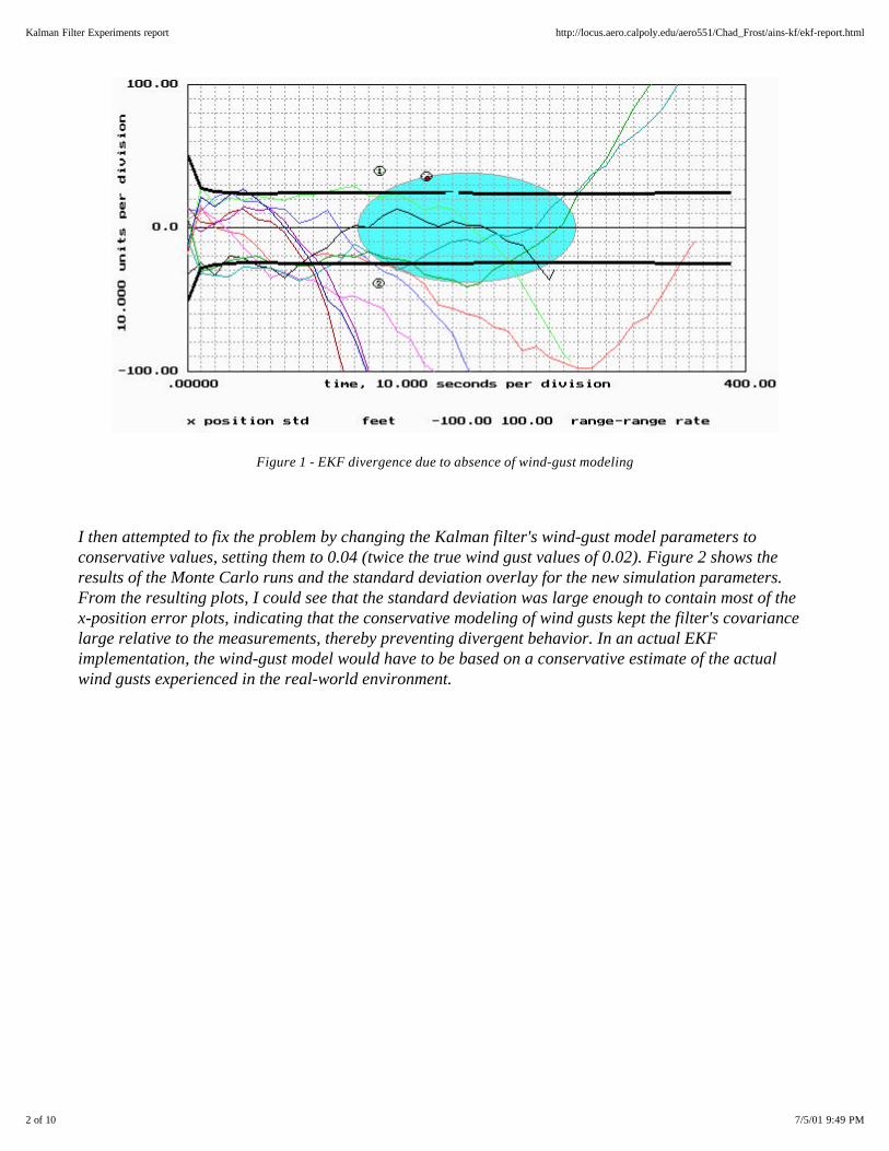
Figure 1 - EKF divergence due to absence of wind-gust modeling

I then attempted to fix the problem by changing the Kalman filter's wind-gust model parameters toconservative values, setting them to 0.04 (twice the true wind gust values of 0.02). Figure 2 shows theresults of the Monte Carlo runs and the standard deviation overlay for the new simulation parameters.From the resulting plots, I could see that the standard deviation was large enough to contain most of thex-position error plots, indicating that the conservative modeling of wind gusts kept the filter's covariancelarge relative to the measurements, thereby preventing divergent behavior. In an actual EKFimplementation, the wind-gust model would have to be based on a conservative estimate of the actualwind gusts experienced in the real-world environment.

2 of 10 7/5/01 9:49 PM


Figure 2 - EKF x-position error with conservative wind-gust modeling

Ramp/Reset Discontinuity

I next investigated the situation where the extended Kalman filter accepted external updates to its estimates on a regular timeinterval. To set up the Kalman filter simulation, I set the time update period to one second, and the number of updates permeasurement to 50. Additionally, to isolate the desired effect from trajectory variations, I set the velocity azimuth to 90 degrees,the wind gust treatment flag to one, and the velocity treatment flag to zero. Figure 3 shows the results of my Monte Carlosimulations for y-velocity, and an overplot of y-velocity standard deviation. The discontinuities that occur when the externalupdates are received by the Kalman filter at 50-second intervals are clear.

3 of 10 7/5/01 9:49 PM


Figure 3 - y-velocity error with external update every 50 seconds

To look at the effect of "overweighting" valid external updates, I set the wind gust uncertainties (x- andy-wind gust error std) to 0.1. My resulting plot of y-velocity error and standard deviation overlay is shownin Figure 4; the updates are considered disproportionately valid by the Kalman filter, causing it to drivethe estimate to the update value every time an update is received. In the cockpit, this behavior would bemanifest by sudden, discontinuous changes in the information displayed to the pilot, and potentially erraticcommands being sent to the autopilot.

Figure 4 - y-velocity error with external update every 50 seconds, and excessive update weighting

Measurement Rejection

After setting the outlier treatment flag to 10 (to cause 20% of the simulation's measurements to be incorrect, with errors ten timesthe normal level), I investigated the effects of different levels of bad measurement rejection on the behavior of the extendedKalman filter. I first performed Monte Carlo simulations without any error rejection; the results are shown in Figure 5. The overlayof the standard deviation shows that the bad measurements are not reflected in the covariance, which decreases as it ispropagated over time. An extended Kalman filter such as this would not provide any warning to the pilot that the filter estimateswere diverging.

4 of 10 7/5/01 9:49 PM


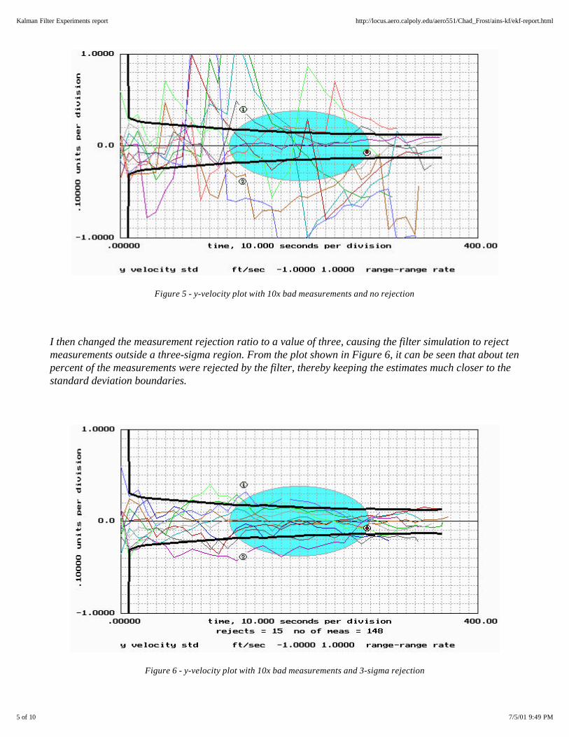
Figure 5 - y-velocity plot with 10x bad measurements and no rejection

I then changed the measurement rejection ratio to a value of three, causing the filter simulation to rejectmeasurements outside a three-sigma region. From the plot shown in Figure 6, it can be seen that about tenpercent of the measurements were rejected by the filter, thereby keeping the estimates much closer to thestandard deviation boundaries.

Figure 6 - y-velocity plot with 10x bad measurements and 3-sigma rejection

5 of 10 7/5/01 9:49 PM


Figure 7 shows the plotted results of changing the rejection ratio to a value of one, causing the filter toreject measurements outside a one-sigma region. As seen in the plot, about 35% of the measurements wererejected. The standard deviation is comparable to that of the 3-sigma rejection level, but a largerpercentage of the estimates fall within the borders.


Keeping the rejection ratio at one, I changed the outlier treatment flag to 20, thereby doubling the errorlevel of the bad measurements. From the results plotted in Figure 8, it is seen that a greater number ofmeasurements were rejected, but the non-rejected measurements produced essentially the same estimatesas before. For comparison, I also plotted the results at this wild outlier level with a 3-sigma rejection level-- the plot is shown in Figure 9. There weren't nearly as many rejected measurements (17 vs. 61) but asseen by the standard deviation plot, the propagated covariance reduced with time.

6 of 10 7/5/01 9:49 PM




If the pilot was provided with an override button to force the Kalman filter to accept rejectedmeasurements known to be valid, the Kalman filter's rejection level could be set tighter than it otherwisecould be, and would allow the filter to be updated successfully even if the filter's estimate drifted offconsiderably. Since this feature would (hopefully) be used infrequently, but would be essential whenactually needed, it would probably be of more practical value than providing the pilot with the ability to

7 of 10 7/5/01 9:49 PM


change the rejection level. Changing the rejection level could actually cause the filter to accept too manybad measurements without the pilot being aware of it.

Effect of Reference Station Geometry on Solution

I changed the extended Kalman filter simulation's reference station positions to be at zero on the x-axis, and separated on the y-and z-axes. Running Monte Carlo simulations (as shown in Figures 10 and 11) demonstrated that the filter was often divergent inits estimation of x-axis position, while it was correct in the y-axis position estimates.

Figure 10 - x-position with reference stations aligned on y-axis

8 of 10 7/5/01 9:49 PM


Figure 11 - y-position with reference stations aligned on y-axis

Re-orienting the reference stations to be aligned along the x-axis, I repeated the Monte Carlo simulations.From the plots in Figures 12 and 13, I found that the y-position estimates were good, while the x-positionestimates were sometimes divergent. These results demonstrated why GPS receivers look at the DOPvalues for the combination of satellites they are receiving, and select the combination affording the bestDOP. A GPS receiver that does not perform such checking, or that can only see satellites that are in pooralignment, could send very inaccurate updates to a Kalman filter.

9 of 10 7/5/01 9:49 PM


Figure 12 - x-position with reference stations aligned on x-axis

Figure 13 - y-position with reference stations aligned on x-axis

10 of 10 7/5/01 9:50 PM


report on extended kalman filter simulation...

Documents