REPORT TO CORRS CHAMBERS WESTGARTH

EQUITY MARKET RISK PREMIUM

MICHAEL MCKENZIE

AND

GRAHAM PARTINGTON

ON BEHALF OF

XTR PTY LTD

REPORT DATED DECEMBER 21, 2011.

Expert Witness Compliance Declaration

We have read the Guidelines for Expert Witnesses in proceedings in the Federal Court of Australia and this report has been prepared in accordance with those guidelines. As required by the guidelines we have made all the inquiries that we believe are desirable and appropriate and that no matters of significance that we regard as relevant have, to our knowledge, been withheld from the Court.

Signed

________________________________ ________________________________

Michael McKenzie Graham Partington

1

Background

This report was prepared at the request of Corrs Chambers Westgarth, who specifically asked us to consider the analysis relating to the MRP in the AER's final decision:

• This includes the following areas of analysis relating to the MRP itself: o Historical excess returns o Dividend growth models o Survey evidence o Market commentary o lmplied volatility (and the'glide path'approach).

• This also includes the following areas of analysis relating to the MRP in the context of an overall rate of return:

o Comparison of regulated asset value with market value o lnformation from broker reports o Comparison of the cost of debt and the cost of equity o Cashflow analysis to meet credit rating metrics.

The written advice should address the following questions: 1. Briefly describe the strengths and weakness of each of the areas of analysis listed

above as a tool for estimating the MRP consistent with the AER's WACC framework. a. For those areas of analysis listed above where you consider that the analysis

does provide useful information about the MRP: i. Briefly summarise the key evidence from this analysis, referring to the

evidence considered by the AER in its final decision and any other research (including published articles in academic journals, academic working papers or conference proceedings) that you consider relevant.

ii. Present (as appropriate) the point estimate or range for the MRP based on this analysis.

b. For those areas of analysis listed above where you consider that the analysis does nof provide useful information, explain why this is so.

2. Consider estimates of the MRP based on any other area of analysis (not limited to those from the AER's final decision).

a. Briefly describe the strengths and weakness of each of these areas of analysis as a tool for estimating the MRP consistent with the AER's WACC framework.

b. For those areas of analysis where you consider that the analysis does provide useful information about the MRP:

i. Briefly summarise the key evidence from this analysis, referring to any research (including published articles in academic journals, academic working papers or conference proceedings) that you consider relevant.

ii. Present (as appropriate) the point estimate or range for the MRP based on this analysis.

c. For those areas of analysis where you consider that the technique does not provide useful information, explain why this is so.

3. Consider the use of both arithmetic and geometric averages when interpreting historical excess returns:

2

a. When determining a forward looking 1O-year MRP estimate for use in the AER's cost of capital framework, consider whether:

i. the arithmetic mean is an overestimate of the appropriate MRP; and/or

ii. the appropriate MRP lies between the arithmetic mean and the geometric mean.

b. Provide reasoning for the conclusion that you reach. 4. Consider the transition from short term volatility to a long term MRP when applying

implied volatility analysis: a. Briefly describe the relationship (if any) between short term volatility and a

long term MRP. b. Describe the strengths and weaknesses of an approach that uses short term

volatility as a tool for estimating the MRP consistent with the AER's WACC framework.

c. lndicate whether Officer and Bishop's'glide path'transition is appropriate. d. Describe any other transition path that you consider appropriate, if any. e. Provide reasoning for the conclusion that you reach.

5. With reference to all the above evidence: a. Explain how you would integrate the evidence across a number of different

areas, including the relative weight to be placed on each source. b. Make a final recommendation on the MRP for Envestra's access

arrangements.

3

The Importance of Definitions

1 The equity market risk premium (MRP) is simply the difference in returns between the risk free asset and the return on an average risk equity investment. In estimating the cost of capital, it is the equilibrium expected market risk premium that is required. It is this equilibrium expected risk premium that makes the marginal investor indifferent between investing in average risk stocks and the risk free asset.

2 For convenience of expression the terms expected, equilibrium, and equity are often dropped. While we also follow this convention, we would like to emphasise that expected and equilibrium are important terms. More specifically, because a forward looking expected value is required, the market risk premium cannot be directly observed, but must be inferred. Further, because it is an equilibrium value, methods that infer the market risk premium starting from current market values assume equilibrium prices, ie. the market is neither undervalued, nor overvalued.

3 We should also like to point out that given the ultimate objective in estimating the MRP is to derive a cost of capital for use in valuation, there must be consistency between the definitions of the market risk premium and the cash flow being valued. A common practice in valuation is to use cash flows measured before allowing for investor level taxes and transactions costs. As such, the market risk premium must also be measured before investor level taxes and transactions costs. Imputation is a complicating factor in the current case, as an adjustment for the value of imputation credits is included in the cash flow.

Determinants of the Equity Market Risk Premium

4 Prior to addressing the issues related to the estimation of the market risk premium, it is first useful to provide an overview of its theoretical determinants. Fundamentally this depends on the investors’ utility function for wealth and the level of market risk. The usual assumption is a diminishing marginal utility for wealth, such that investors are risk averse, but their absolute level of risk aversion declines as their wealth increases. At a less abstract level Damodoran (2010) provides the following list of the determinants of the market risk premium:

1. Investors’ risk aversion – an ageing population or changes in investors’ intertemporal consumption preferences will cause their level of risk aversion to alter.

2. Economic Risk – risk premiums are lower in countries with stable economic fundamentals.

3. Information – improvements in the quantity and quality of information leads to lower equity market risk premiums.

4. Liquidity – large risk premiums will be demanded for investments where exit costs are high. Similarly, in periods of recession or crisis, the MRP will increase as liquidity falls.

4

5. Catastrophic Risk – the probability of such ‘black swan’ events is low but positive nonetheless and as such, the MRP must reflect the risk of such black swan events.

6. Behavioural issues – since the equity market risk premium is an expectations based metric, these expectations will be subject to the plethora of biases which form the basis of behavioural finance/economics. Thus, the MRP may be unrealistic or irrational and in a bull (bear) market, and investors may extrapolate high (low) observed returns into the future.1

5 While other taxonomies are possible, the main point is that the market risk premium has fundamental determinants (whatever they may be) and these may change over time, in which case the market risk premium changes. The key is whether they are mean reverting or not. If they are, some average risk premium exists given a sufficiently long time horizon.

Measuring the Equity Market Risk Premium

6 While the equity market risk premium is an apparently straightforward concept, it is extremely difficult to measure accurately. The reason for this is simple - the MRP is an expectations based metric and measuring the expectations of investors is fraught with difficulty. As Brealey et al (2005, p. 154) put it: “Do not trust anyone who claims to know what returns investors expect.”

7 A number of approaches have been developed for estimating the equity market risk premium. These can be broadly grouped into surveys, the construction of forward looking (implied estimates) based on valuation models, estimates based on historical returns, and estimates based on volatility models. There is also analysis based not on data, but on utility theory. Utility theory has been utilised to appraise the reasonableness of empirical estimates of the MRP. The main of application utility theory has been in relation to historical return estimates of the MRP. Therefore, we discuss the results of utility analysis in the context of historical return estimates of the MRP.

8 We shall consider each of the methods above, but there are some methods that we exclude from consideration. We do not consider the use of predictive models of return based on dividend yield, even though distinguished researchers have (such as Fama and French, 1988). Spurious regression can be a problem here and researchers, such as Fisher and Statman (2000a) and Goyal and Welch (2003), find little evidence of predictive ability in such regressions. In our opinion, this is still a developing area of research, rather than a well developed practical tool, although its importance is growing (see Cochrane 2011). Neither do we consider the information in index dividend swaps, nor exchange traded futures on

1 Risk premiums and asset prices are inversely related – ie. high stock prices mean a lower return, thus the excess over the risk free rate is low. Investors will pay a lower price for risky cash flows compared to risk free cash flows – how much lower is a function of the MRP. When risk premiums rise, investors are prepared to pay less for the same set of risky cash flows, ie. stock prices fall.

5

the index dividend. Such data provides information on both variation in expected dividends and returns and the challenge is to separate the two. Research on this is promising, but is still too early to tell whether the information provided is useful.

9 Some of the evidence that we consider is international in nature and much work has been done in the U.S. A natural question is why international evidence is relevant to the Australian market risk premium. The answer is that capital markets are at least partially integrated and hence there are likely to be common elements across markets in the behaviour of market parameters such as the MRP. Indeed Damodoran (2011), a well respected authority on valuation, takes the Australian market risk premium to be the same as the U.S. market risk premium, which he currently estimates to be 5%.

10 Empirical estimation of the market risk premium commonly results in a distribution of possible risk premiums, or returns. So a natural question is which measure of the central tendency of the distribution should be used - the mean, median, or mode. There is no compelling reason to assert the superiority of one measure over another. Common practice has been to use the mean, in part because it is the most mathematically tractable measure. As a consequence, where the returns are skewed, the MRP estimate will be biased relative to the other two possible measures. This can be a particular problem in small samples where the mean can be strongly influenced by one or two extreme observations. Where large samples are used, we anticipate that differences between the three measures of central tendency be small. A much bigger problem is likely to be a large standard error in the estimate of the mean. Another important source of differences in the estimated MRP is whether an arithmetic or geometric average is used and we discuss this issue later in this report in the context of the historic risk premium.

11 One further important measurement issue is the proxy chosen for the risk free rate and whether it should be a short or long dated government security. There is a well developed consensus that for long term investment decisions, such as in capital budgeting, the appropriate choice is the long dated government bond. Thus, where there is a choice of risk free proxies we report results for the MRP using government bonds.

1. Equity Market Risk Premium Estimates Based on Past Data

12 While the required equity market risk premium is a forward looking (ie. ex-ante) concept, by far the most common technique used to generate estimates of this premium is an examination of past data and some form of historical averaging, resulting in a backward looking (ie. ex-post) realised estimate. An advantage of using averages from historic data, particularly in a regulatory context, is that it is relatively transparent. The choices that can be made (most of which are discussed below) are generally well defined and most of their consequences can be readily investigated. Historical estimates have also been extensively studied and as a consequence are quite well understood. There is also plenty of

6

international evidence which allows a cross check on the reasonableness of Australian estimates. The historical approach also has support as the benchmark method for estimating the risk premium in Australia (see Hathaway, 2005, and Officer and Bishop, 2008).

13 Despite its widespread use and popular appeal, a significant number of estimation issues confront the researcher when attempting to estimate the equity market risk premium using historical data. These problems are by no means trivial, and Goetzmann (in Welch, 2000) goes so far as to argue that the estimation of a ‘pure’ estimate of the historical equity premium may be impossible. We now turn our attention to consider each of these issues in turn.

The Equity Risk Premium Puzzle and Survivorship Bias

14 The equity risk premium puzzle refers to the observation that the estimated historic risk premiums are too high, that is to say they are too high relative to the predictions of utility theory2 (see the seminal contribution of Mehra and Prescott, 1985). Economic theory has great difficulty in explaining observed MRP estimates even assuming quite high degrees of risk aversion and different modifications to standard consumer choice models (see Cochrane, 1997, and Siegel and Thaler, 1997). The question is whether realised equity returns are higher than equilibrium expected returns for some reason, and so lead to overstatement of the MRP, or whether there is something missing from the theory.

15 Damodoran (2011) observes that the explanations for the equity risk premium puzzle have generally focused on:

1. Survivorship bias which arises because returns are estimated from the stock exchanges and stocks that have survived, the winners so to speak. Thus many of the negative returns are missing from the historical record. Survival is a consequence of a goodly share of good news and good luck, which naturally results in inflation of realised returns.

2. The MRP is a function of not only observed volatility, but also potential volatility. In particular investors expect to be compensated for rare catastrophic (so called black swan) events - see Reitz, 1988).

3. Personal taxes have generally declined since World War II, thus reducing the pre-tax return that investors demand. We note that a similar argument can be made with respect to transactions costs. As required returns fall prices go up, thus inflating realised returns.

4. Alternative preference structures – the MRP puzzle is a direct result of the assumption of constant relative risk aversion (CRRA) assumed for the utility functions of investors. The high MRP can be explained by alternative utility functions that

2 To avoid confusion we should point out that utility in this context does not refer to regulated utilities, but to the economic concept of the satisfaction obtained from wealth and consumption.

7

allow for an aversion to consumption changes across time, or habit formation, explain the high MRP.

5. Myopic loss aversion – investors who receive constant updates on equity values, perceive more risk in equities.

16 Welch (2000) adopts a simpler approach to summarising the arguments to explain the equity premium puzzle. He argues that either high equity premia are necessary to induce investors to participate in the stock market, or investors expected returns have fallen. The former suggests the equity premium will remain as high in the future as in the past. The latter suggests the expectation of much lower returns in the future (for example, Heaton and Lucas (1999) argue increased diversification has reduced investor risk and so the risk premium).

17 The equity risk premium puzzle suggests that estimates of the market risk premium, based on historical data, may be overstated relative to true expectations. Of the various explanations proffered to explain the premium, arguably the survivorship bias has received the most attention. Jorion and Goetzmann (1999) argue that survival bias is a significant estimation issue and attempt to adjust for the effect of markets that have been closed or suspended. They find that the U.S. market is a winner and that realised returns are upward biased by between 25 to 70 basis points. Siegel (1999) argues that historical returns underestimate real returns on risk free assets due to unanticipated inflation. He also argues that historical returns on equity are an overstatement of returns actually realised because of historically high transaction costs and the historical lack of low cost opportunities for diversification. Consequently, he suggests the future MRP will be lower than that suggested by the historic record.

18 According to Tables 1 & 2 in Dimson, Marsh and Staunton (2011), the historic record suggests that Australia is the luckiest of countries. Over the period 1900 to 2010 it has the highest real equity return around the world and the second lowest risk (standard deviation of those returns).3 As well as the having highest returns, Australia also has the highest geometric mean MRP (5.9%) despite having the second lowest risk.4 The obvious question is whether this is plausible and three explanations occur to us. One explanation is that investors in the Australian market have had a very high risk aversion relative to everywhere else and thus, we have a larger equity risk premium puzzle than elsewhere. A second explanation is that there has been plenty of luck in the lucky country inflating realised returns. If so, investors have been pleasantly surprised by receiving more than their expected risk premium. A third explanation is measurement error and survival bias. We 3 We note that Australia’s lead would likely have been even bigger if any allowance had been made for the return from imputation credits. 4 However, the arithmetic average MRP at 7.8% is only the fourth highest. This is because the arithmetic mean is a function of the geometric mean and the standard deviation of returns (volatility). Australia’s low volatility thus drags down the arithmetic mean.

8

think the latter two explanations are the more likely ones. In particular, Brailsford, Handley and Maheswaran (2008) highlight problems of data quality in the first half of the twentieth century including survival bias and other sources of return overstatement.

What is the market?

19 The theory underlying CAPM is unambiguous in terms of the choice of index used to represent the market – it should represent all assets in the economy weighted by their relative values. In reality, no such index exists and therefore the index should be a value weighted index representing the broadest range of sectors in the economy. In practical terms, this translates into the use of a broad based equity market index.

20 The use of an equity market index to proxy for the market brings with it two well documented problems. The first is the potential for survivorship bias in the index, as stock returns should incorporate those firms that were acquired or went bankrupt. On a similar theme we note the bias that arises from changes to the constituents of the market index, whereby poorly performing stocks are systematically excluded from the index at regular intervals and replaced. The second problem is the perennial issue of coverage. The wider the index, the more stale price information it includes from small stocks, while the narrower the index, the more relevant the price information, but at the expense of coverage.

21 The choice of market index matters as noted by Fernandez (2009, p. 6) who argues that the main driver of differences in estimates in the range of textbooks surveyed is driven by the choice of stock index.

Which measure of central tendency?

22 As discussed earlier, the choices for measures of central tendency of the return distribution are the mean, median, or mode. The standard choice in relation to historic estimates of the MRP has been to use the mean, which is the expected value mathematically speaking. At a practical level, this is likely to be a reasonable choice in large samples. The problem is that large samples tend to be taken over the broad sweep of history, which creates other problems. It is clear, however, as the time frame used becomes shorter and the sample gets smaller there is a greater risk that outliers and skewed distributions will lead to a bias in the mean.

The Return Measurement Horizon

23 The Capital Asset Pricing Model is a one period model, however the time dimension of that period is unclear. Conceptually, it is the price setter’s investment horizon and it is commonly assumed that there is a match between the asset life and investor’s planning horizon. In practice however, returns are usually expressed as per annum returns.

9

24 The use of annual returns brings with it issues when scaling the estimate to longer time horizons (for example, a 5 year regulatory period). One solution to this problem would be to use returns over a longer period to avoid having to scale (such as 5 year returns), although this approach would result in very few data points given the data available. In essence, this is the same as Blume’s (1974) unbiased estimator although one key difference is that Blume was undertaking a Monte-Carlo study based on 1,000 separate samples of 80 observations. The use of a large dataset gives similar standard error across the different methods considered. In reality however, the standard error would be much higher for the unbiased estimator due to the smaller sample size. For this reason, we consider that Blume’s (1974) unbiased estimator is unlikely to be a superior alternative to the arithmetic average. The size of the standard errors observed using real world data are so great, that any reduction in bias is likely to be more than offset by reductions in the precision of the estimate. As such, we would argue in favour of the more traditional measure.

Data Adjustment and Removal of Outliers

25 A number of authors have argued that where there are events in the data sample period that are not expected to reoccur in the future, then they should either be excluded, or adjustments made to the estimate. For example, Dimson, Marsh and Staunton (2008) find a long-term upward trend in price-dividend ratios and price-earnings ratios. They argue that such trends are unsustainable and necessitate some form of adjustment to the estimated equity market risk premiums. Hathaway (2005) adjusts for this effect of inflation of price earnings ratios in Australia post 1980. The danger with such adjustments is that they tend to be ad-hoc.

26 While the removal of outliers is a common practice in statistical analysis, it will most likely prove very problematic in the current context. Taken to extreme, it is possible to view each period of the market as unique. For example, the doubling of the price to earnings ratios in the 1980’s and the financial market deregulation of the same period, the OPEC oil crisis and stagflation of the 1970’s, the October 1987 crash, the post-WWII boom period, and so on. All such episodes are arguably unique and not to be repeated. As such, to remove outliers from the data is to introduce an extremely arbitrary bias to the data as it is entirely unclear exactly what does or does not constitute such an event.

How to Calculate Excess Returns

27 A fundamental issue for the estimation of historical risk premiums is the manner by which the excess returns are calculated. As Hathaway (2005) observes, the market risk premium could be estimated by calculating the annual equity return less the redemption yield on the risk free asset at the beginning of the year. The risk premium then, is simply the average of these differences. The alternative approach is to estimate annual equity returns over a window of several years and then average those values. The market risk premium in this case is the average equity return less the yield on the risk free asset at the start of the

10

period. Hathaway (2005) invokes the (arguably implausible5) assumption of unbiased expectations and argues in favour of the latter method. Hathaway reasons that the average market return may be viewed as an estimate of the expected risky asset return. Therefore, by subtracting the risk free rate, an unbiased estimator of the risk premium is derived. In subsequent analysis though, Hathaway (2005) does consider both estimation methods. While yields to maturity have much to recommend them as measures of the risk free rate, we note that some researchers such as Dimson et. al. (2002) use realised returns.

Arithmetic or Geometric Mean

28 A fundamental decision when generating a historical estimate of the equity market risk premium is whether to use an arithmetic or geometric average of excess returns. It is useful in this context to write the following relation between the actual return and the expected return:

Actual return = Expected return + Surprise return

29 Statisticians would label the surprise return as the error, which measures how far the expectation was from the return experienced ex-post. Common sense would suggest that if the expectation was unbiased, such that the surprises were equally likely to be positive or negative, then on average they would sum to zero. So repeatedly measuring the actual returns and taking the arithmetic mean should give the expected return. More formally, a statistician would recommend the arithmetic mean if the observations of actual returns were independent and drawn from a stationary distribution with a finite variance. Unfortunately, reality does not perfectly match the statistician’s requirements.

30 The first issue is that returns compound through time and while the arithmetic average does not capture this, the geometric average does. A simple and commonly cited example serves to highlight the difference between the two approaches. Assume that you invest $100 and it shrinks to $50 by the end of the first year, this equates to a simple -50% return. In the second year the invested amount grows to $100 and thus gives a simple 100% return for that year. The actual portfolio return over the two year period is 0% and this is the geometric average, however, the arithmetic average return is 25%, ie. (-0.50 + 1.00)/2. The geometric average represents the actual investment returns from a buy and hold investment strategy, while the arithmetic average is earned by a strategy that rebalances the investment to a fixed amount each year. Except in cases such as a one period investment, mathematically the geometric mean is less than the arithmetic mean.

31 The decision as to whether to use the arithmetic or geometric average is complex. Arithmetic averages are certainly more popular. For example, Bruner et al (1998) find that

5 The assumption that return expectations are unbiased is a major weakness of this approach given the lessons of behavioural finance.

11

71% of the textbooks surveyed used arithmetic averages to estimate the MRP, while only 15% use geometric averages (14% did not specify the averaging process used). The arithmetic mean is also consistent with the assumptions of asset pricing models such as the CAPM, which is a single period model (as discussed previously, the length of this period is assumed to be the investment horizon, which is undefined in the standard model6). Further support for arithmetic averages may be found in the argument that investors form their expectations of observed returns based on actual returns (if stock price moves 1.00 to 1.10, it is viewed by investors as a 10.0% return, not 9.53% continuously compounded). Finally, the arithmetic average is arguably appropriate when attempting to find the best representation of expectations that are formed based on historical data (ie. the probability weighted outcome, or arithmetic average, is the correct estimate of the most likely outcome for the next period). Note that this does assume each observation is an independent draw from a stable distribution. Returns are known to be negatively serially correlated however (see Fama and French, 1988), in which case the arithmetic average will overstate the premium.7

32 The problem with the use of annual arithmetic averages, is that compounding an arithmetic average will lead to a bias, while compounding a geometric average may not.8 One alternative is to use returns estimated over the period of interest (for example, 5 or 10 years), but given the aforementioned problems with a century of annual data not providing sufficiently accurate estimates, this is not a viable option.

33 Indro and Lee (1997) suggest a weighted average of the two averages is appropriate, with a higher weight on the geometric the longer the time horizon over which the premium is to apply. Dimson, Marsh and Staunton (2003), Hathaway (2005) and Campbell (2007) take a somewhat different and more novel approach. They estimate the geometric average stock return for a sample of data and then convert it to a forward looking arithmetic average MRP. The general relationship between an arithmetic average (RA) and a continuous or

geometric average (RC) is given by the approximation RA RC 0.5σ .

34 Thus, the arguments suggest that a geometric average is clearly inappropriate for the purposes of characterising expectations, however the issue of scaling arithmetic averages introduces a bias when compounding over longer horizons. While characterising the past data using geometric averages and converting it into a forward looking arithmetic average

6 This could be one year, the regulatory period of 5 years, 10 years or some other length of time contingent on the underlying assumption as to the time horizon of the representative investor. 7 Note that one theoretical argument that is occasionally raised in favour of continuous returns is that they are more mathematically tractable and also more likely to conform to the normality assumption. While this is true in higher frequency data (daily or less), the assumption of continuity becomes tenuous for less frequently sampled data, such as the annual data that is typically used in risk premium studies. 8 Blume (1974) actually suggests that caution is required when extrapolating either arithmetic or geometric average returns to a longer horizon as both are biased - overestimated in the case of arithmetic and underestimated in the case of geometric.

12

using current market volatility is appealing, the problem is that the validity of this adjustment relies heavily on the volatility estimate. It is unclear exactly what the ‘current’ market volatility is and any estimate will be sample dependent, highly variable and estimated with some degree of imprecision. All of which means that in trying to adjust for the compounding error, you are introducing another form of unknown error and it is entirely possible that the latter may be larger than the former. Until such time as the bias inherent in the volatility adjustment process is more fully understood, we recommend using the arithmetic average. This recommendation however, is subject to the caveat that due recognition be given to the likely overestimation bias inherent in the use of the arithmetic average.

Structural Changes Over the Data Sample Period

35 The use of annual data to accurately characterise the distribution of the equity risk premium, requires a very long sample period. We note that many studies have used over a century of data. The use of such a long data series however, raises an important issue as to how applicable past historical return estimates are to the current period. In effect, the issue is whether any structural changes have taken place over that sample period such that data from one regime is no longer relevant in the current estimation period.

36 Hedberry and Lim (2003, p. 21) argue that the Australian economy has seen a number of structural changes9, including:

• the floating of the Australian dollar; • deregulation of the banking and financial systems ; • integration of the Australian economy into the global market; • the elimination of many forms of tariff protection; and • a major overhaul of the tax structure.

37 This last point is perhaps the most important of these changes in the current context. In

Australian, there have been substantial changes to the capital gains tax regime, as well as to the corporate tax and personal income tax rates, which have been substantially reduced. Since 1987, there have also been a number of major changes to the tax treatment of dividends:

• A dividend imputation system was introduced on July 1, 1987;

• A tax on superannuation funds was introduced from 1st July, 1988;

9 More generally, a wide range of possible causes of structural breaks have been discussed in the literature. These include: the increase in the range of investment opportunities available to investors (index funds, hedge funds, private equity, emerging market funds and private equity funds etc.) resulting in increased diversification opportunities leading to a lower required return to holding stocks; improved opportunities for risk management through a greater range of derivatives; global interest rate and inflation stability; and, improvements in information technology. These are all commonly cited reasons as to why historical data may no longer be relevant and making adjustments to account for such factors is all but impossible.

13

• In 1997, a 45 day holding period around the distribution of franking tax credits was introduced;

• In July 2000, surplus credits became refundable in cash.

38 The first of these changes is particularly problematic as there is no single, precise and robust estimate for the value of imputation credits that is universally viewed as being correct. For these reasons, it is common to only consider the cash value of dividends and not include a value of imputation tax benefits when constructing stock return indexes. It is also common practice to ignore imputation credits in estimating the discount rate for valuations as surveys show (see Lonergan, 2001, Truong et. al., 2008, KPMG, 2005, and Bishop, 2009). In some cases this is because of uncertainty over the value of the credit and how to properly adjust discount rates. In other cases, the credit is ignored because it is not thought to be valuable.

39 Since the valuation in this case makes adjustment for the imputation credit in the cash flow, the consistency principle requires that this be built into the investors return. Logically, therefore, the value of imputation credits should be added to returns over the period from the time imputation was introduced. With the current regulatory value of gamma at 0.25, the effect is small. Handley (2011) for example allows for a gamma of 0.2 and this makes no difference to risk premiums for periods staring before World War II and ending in 2009. For periods starting after World War II and ending in 2009 the effect is an increase of 20 to 30 basis points. If, in reality, this effect was already in returns, it is so small that it would most likely get lost in the noise of the data and so be undetectable.

40 It is instructive to consider what would likely happen to the MRP on the introduction of imputation credits. All other things being equal, it would cause the MRP to fall somewhat as imputation increases investors’ after personal tax returns. If their required after tax returns remained constant the observable component of pre-tax required returns would fall, and this would be offset by the “invisible” component of imputation credits. In theory then, the estimated MRP based on the observed component of returns would also be smaller. In reality, we expect this effect could easily be undetectable given the noise in returns. Thus, while adding back the imputation credits is correct from a theoretical point of view, in practice it may not prove to be a useful refinement. As Handley’s analysis shows the impact on the estimated MRP will be contingent on the length of the data series used to estimate the MRP.

41 More generally on the issue of structural breaks, the variability of the equity market risk premium means it is difficult to successfully identify structural shifts as statistically speaking, the tests lack power. For example, Gray (2001) uses t-tests of differences in means for the Ibbotson 1883 – 2000 data. Lally (2005) observes that, “this test suffers from the crucial limitation that it is virtually powerless to detect even quite substantial shifts in the

14

premium”. Hancock (2005) however, does find evidence of structural breaks in time series tests using an ARMA model.

42 While it is difficult to establish statistically significant shifts in the risk premium, it is clear that there have been considerable improvements in the accuracy and coverage of the data relative to distant history. It is also clear that there have been changes, which are likely to have led to structural shifts in risk premiums. In our opinion the weight of evidence discussed here and in other parts of this report suggests that the long run average MRP has declined.

Stationarity of the Distribution

43 One of the most contentious issues when estimating the equity market risk premium relates to the time period over which the estimate should be generated. Many authors have argued that in order to reliably estimate the historical equity premium, a clear case can be made for the use of data sampled over a long time horizon. The logic underlying this assertion is that the volatility of stock returns is so high, that it is hard (if not impossible) to measure the mean historical premium with precision without long-run data. On this point, Dimson, Marsh and Staunton (2003) observe that even with “102 years of data, the potential inaccuracy in historical risk premiums is still fairly high”. The standard error is commonly used as a measure of the inaccuracy of an estimate and, for ‘shorter’ time periods, it can be larger than the estimate itself (see Table 7 in Damodoran, 2010). For example, Handley (2011) estimates an arithmetic mean risk premium:

• of 6.2% (with a standard error of 1.5%) for 127 years from 1883 to 2009;

• of 6.2% (with a standard error of 3.2%) for 52 years from 1958 to 2009;

• of 5.2% (with a standard error of 4.1%) for 22 years from 1988 to 2009.

44 A number of assumptions underlie this argument in favour of long data sample periods. The first is that a premium estimated over a sufficiently long period of time must be ‘precise’. Second, the estimated risk premium will be stable and, where deviations occur, the estimate will (eventually) revert to the long run average.

45 Each of these points is questionable. The evidence suggests that using long time periods of data will not lead to a consensus on the correct risk premium. In fact, estimates that use long data histories produce estimates that vary widely. Further, any notion of mean reversion is questionable as issues remain as to which mean does the premium revert and over what time period (if indeed it does revert, which it may not in the presence of structural breaks). These factors mean that exceptions to mean reversion will almost certainly exist as a new mean becomes the norm at some stage during the sample period.

46 By far the greatest deficiency to the argument in favour of the long data sample period is questions over the relevance of such data. As Welch (2000, p 5) puts it, “50-year old equity

15

premia may have little relevance to the world today”. Thus, the task at hand involves not only generating a reliable MRP estimate, but ensuring that none of the underlying fundamentals have changed, no structural breaks have taken place, and so on.

47 There is an abundance of evidence however, to suggest that the past will not be repeated and a variety of reasons exist to support this view. Firstly, most long run studies of the equity risk premium focus on either the U.S. or the U.K.. As Bodie (2002) observes, “(t)here were 36 active stock markets in 1900, so why do we only look at two? I can tell you — because many of the others don’t have a 100-year history, for a variety of reasons.” Jorion and Goetzmann (1999) and Dimson, Marsh and Staunton (2000, 2003) both observe that the 20th century proved to be a period of remarkable growth in the U.S. economy, probably exceeding the expectations held by U.S. investors in 1926. As a consequence, it may be argued that any long dated historical series overstates a forward view of the equity risk premium.

48 More specifically, a number of important changes have taken place in the markets, which cast doubt on the reliability of past data. One such change has been to the leverage of the equity markets, which has risen dramatically since deregulation. Further the composition of the markets has changed both in terms of the stocks listed (eg: the ascendency of technology stocks) and also the composition of the investors active in the market. This latter point is particularly important as little thought has been given to the ascendency of the professional investor and their impact on the market. To highlight this point, Figure 1 presents information on the composition of trading activity in the U.S. market post WWII. The percentage of ownership (measured on the left hand axis) across various different groups (labelled at the right) for each year (measured on the bottom axis) is given. The stock market prior to WWII was clearly dominated by retail investors, the majority of whom were arguably unsophisticated. The largest area at the top of the figure represents households and this group clearly dominates in the early 1940’s with a share of ownership of more than 90%. By the end of the sample period however, ownership had clearly shifted in favour of the institutional investor, who now dominate the market. This change came from the rise of pension funds during the 1970’s and mutual funds during the 1980’s. More recently, it has been a steady influx of sophisticated international investors, as well as the rise of hedge funds and ETFs. All of these changes mean that the data prior to 1970 was determined by a very different set of investors than over the last 40 years.

16

Figure 1 Share of US Corporate Equity Market

Source: Kostin (2011)

49 It is interesting to note that Welch (2000a) observed that the survey data finds that small investors (who dominated trading in the stock market in the early years) tend to expect equity premiums between 10 percent and 15 percent per year.10 In contrast, professionals and organisations tend to be more conservative in their assessment of the MRP.11

50 The impact of this change in the composition of active participants in the market is yet to be fully explored. Given the evidence however, it is likely that professional investors have a far more realistic expectation of returns from investing in the share market.

51 On a similar theme, Bassanese (2004) argues that the selling down of equity holdings acquired by the baby boomers to finance their retirement may depress equity prices and cause the equity market risk premium to fall.

52 On a more practical note, there are very real deficiencies with the early data. For example, Goetzmann and Ibbotson (2005) construct a complete index of capital appreciation returns for the New York Stock Exchange from its inception (1792) to the present but find that the absence of a riskless rate pre-1925 renders the estimates near meaningless. Further, the U.S. market prior to WWI arguably resembled that of an emerging market with relatively infrequent trading – certainly a far cry from the superpower that emerged after WWII.

53 Early stock market index data also tends to be based on only a few stocks. For example, Brailsford et al (2008, p. 76) reports that the long dated Australian index series used in

10 Welch (2000a, p 6-7) reports that surveys of small investors find expected equity market returns of 16-22%. 11 Welch (2000a, p 7) reports that surveys of institutional investors find an expected equity premium of 3-6%.

% Ownership by Group

Households

Mutual Funds

Pension Funds

Gov’t Retirement Funds International Investors

Hedge Funds ETFs Other

17

Officer (1989), Dimson, Marsh and Staunton (2003), Hathaway (2005), Hancock (2005) and also their own work, used an index which was based on only 5 stocks in 1875 and 12 in 1905.

Conditional Estimates of the Equity Market Risk Premium

54 The discussion of the previous sections suggests that attempting to estimate an equity market risk premium from a long series of data, risks using poor quality data and crossing structural breaks. One alternative is to estimate a equity risk premium which is conditioned on the current state of information.

55 Since the cost of debt is allowed to vary with changing credit spreads, arguments in favour of a conditional estimate can also be made on the basis that it is more logically consistent with the way the cost of debt is measured. The catch is that changes in credit spreads are readily observed, but changes in the MRP are not.

56 Other arguments in favour of a conditional estimate rest on the observation that the determinants of the market risk premium (as previously discussed) are not fixed and may well vary over the forthcoming regulatory period. Damodoran (2010), for example considers September to December, 2008 as a period of an extreme movement in the index and reports that the equity market risk premium was found to vary from 4.20% to 8.00%.

57 More generally, Gailbraith (1993) observes that financial memory is particularly short lived and so a long series of returns data may not be appropriate if people are only cognisant of the last few years in setting their estimate of the equity market risk premiums. This argument however, works both ways. Depending on how short term their memory is, investors may well forget the last crisis and revert to some long run risk premium as soon as the crisis is over. It should also be pointed out, that investors may also frame their expectations relative to opportunity cost. Given the extremely low interest rates that currently prevail in the global markets, investors may have similarly low expectations for equity (despite the crisis increasing risk).

58 These arguments aside, there are some compelling reasons to avoid the use of conditional equity market risk premium estimates. Firstly, Hathaway (2005) argues that there is no obvious term structure for equity returns, in the same way that bond yields have a term structure. In fact, he argues that it is ‘safe’ to say that the mean return per period is the same for short term investments as it is for long term investments (an argument therefore in favour of an unconditional approach).

59 Further, for firms with long term investments and cash flows that extend over many years, using conditional risk premiums can skew the investment process such that too much investment is initiated in periods where risk premiums are too low and vice versa for period

18

where risk premiums are too high. Hathaway (2005) argues that a preferable solution may be to compute normalized risk premiums (either a historical average “implied” premium or a fundamental-adjusted implied premium), which would provide more continuity to the investment process.

60 Some authors have suggested using a longer sample of data, but with a higher weight placed on more recent data. The effect of this however, will be to increase the standard error of the estimate and so it is not a viable option. For example, using the last 10 years of data is an extreme form of weighting in which the weights placed on past data are set to zero and so effectively you have a short data history.

61 For regulatory purposes, it seems undesirable to have conditional estimates of the market risk premium varying, sometimes sharply from period to period. The general view seems to be that a stable long run MRP (approximating the unconditional mean) should be used for regulation.

Summary

62 Despite all of the issues and available choices discussed above, the estimates of the Australian arithmetic market risk premium are not wildly divergent, relative to the implied MRP discussed in section 3. Ignoring adjustments for imputation, they range from 4.5% Hathaway (2005) to 7.9% Dimson et. al.(2011). Given the standard errors typical in such estimates, it is doubtful if we could conclude that these estimates are significantly different. Furthermore, most authors do not provide a single estimate, but rather a range of several alternative estimates, so there are plenty of MRP values to choose from. In general, the estimates are high relative to the rest of the world, where 5% would be a common estimate. There are also plenty of reasons why the historic average MRP estimates might tend to be upward biased and we think that this is likely to be the case. The financial crisis is likely to have temporarily inflated the MRP, but this could not be accurately measured using historic averages, or probably any other technique. We also find Brailsford et al’s (2008) arguments about the vagaries of the early data quite convincing.

63 In our opinion, estimates from historic analysis of the MRP provide no compelling reason to have deviated from the long-standing regulatory consensus of a 6% MRP. In this respect, we agree with Gray and Officer (2005) who state, “(w)e recognise that it is likely that the MRP is not stationary and likely to vary under different economic conditions. However, the fact that there is no adequate theory underlying the variability of MRPs makes it dangerous to adjust an MRP estimate simply because another year or two or three of data alter the estimated mean. For example, a year ago the 30-year mean excess return was less than 6%, leading some to call for a reduction in the MRP used by Australian regulators. Now, the most recent 30-year mean return is 7.7%. We do not advocate increasing the MRP now for the same reason we did not advocate reducing the MRP estimate last year. The problems of the

19

theory and measurement of MRPs suggest a conservative approach – a regulator should be very careful about making any changes without compelling evidence.” We do note, however, that the 6% estimate may prove to be too high in the long term.

2. Surveys

64 Since the equity market risk premium is an investor expectations based metric, it would seem that the most logical method by which estimates may be garnered is to ask investors what their expectations are. This however, is easier said than done as it is unclear exactly who the appropriate group to survey is and whether their responses match their true beliefs. In terms of selecting a survey group, obviously it is not possible to survey all investors and so a subset must be chosen. Fund managers, financial analysts, corporate financial managers, and finance academics have typically been the focus of risk premium surveys, although surveys of individual investors have also been conducted.

65 A substantial body of survey evidence comes from the U.S., and the results suggest a generally falling risk premium, which did rise during the GFC and then resumed its downward trend. One of the better known U.S. surveys is a survey of senior finance managers (CFO’s) that has been conducted quarterly from the 2000 onwards by Graham and Harvey (current version 2010). In our opinion this is both relevant to the current case and is arguably one of the more reliable surveys for the following reasons. First, the authors have a reputation for high quality research. Second, the return estimate is for a ten year horizon and comes from managers who are responsible for using this information in making investment decisions. Third, while the response rate is low at 8%, this represents a substantial number of responses with an average of 333 respondents each quarter. Fourth, Graham and Harvey (2010) make a case, supported with evidence, that response bias is not a major problem in their study. Fifth, continuing use of the survey over 41 quarters suggests a reliable survey instrument and even if there are problems in the framing of questions they will be the same from period to period. Consequently, the observed changes through time are less susceptible to framing issues. Finally, the authors do not overstate their results - their claim is that they have a measure of expectations, but not that it is necessarily the true market expectation.

66 Graham and Harvey state that respondent CFOs forecast the expected market return as a buy and hold return and thus the survey results should be interpreted as measuring geometric averages. They conclude that as at June 2010, the average market risk premium for the S&P500 has fallen back from a GFC high of 4.7% to 3.0%, a level comparable with that prevailing in late 2006 and early 2007, and below the average over the decade of 3.5%. While the estimated risk premium has fallen below the decade average, the dispersion of opinion across managers, reflected in the standard deviation of responses, remains above the decade average, with a standard deviation of 3.1% compared to the decade average standard deviation of 2.6%.

20

67 This data suggests that increases in the MRP during the financial crisis have been reversed.

It is also evident that managers are using MRPs that are below the long run historic average stretching back to the beginning of the twentieth century. The long run arithmetic (geometric) average risk premium for the U.S. from 1900 to 2010 was 6.4% (4.4%), (see Dimson, Marsh and Staunton, 2011). The managers’ survey MRPs are much closer to historic returns from the last half century or so. Ibbotson Associates data from April 1953 to July 2010 inclusive, gives an average arithmetic (geometric) market risk premium of 4.2% (3.4%).12

68 The MRP in textbooks, which is typically an arithmetic average, has also declined. Fernandez (2009) surveyed 150 corporate finance and valuation textbooks and reported that the five year moving average of textbook MRPs has declined from 8.4% in 1990 to 5.7% in 2008 and 2009. The same trend is also evident in the MRPs from surveys of academics in the U.S.. Welch (2000a) reports an arithmetic average MRP of 7%, based on surveys of academics in 1997 and 1998. This had fallen to 5.5% when academics were surveyed in 2001 (see Welch, 2001) and was only slightly higher at 5.7% at the end of 2007 (see Welch, 2008). Fernandez (2011) surveys 1,503 academics, financial analysts and company managers and reports a U.S. risk premium of 5.5% in 2011.

69 In Australia, the surveys suggest a consensus risk premium of 6% and provide no evidence that this is any higher in 2011. The surveys are not specific about whether the estimates represent geometric or arithmetic averages, or whether they represent a premium over treasury bonds or notes.13 However, since the general context is valuation and capital budgeting, with the MRP to be used in the CAPM and calculation of the WACC, we may reasonably infer that these are arithmetic averages of the MRP relative to bonds.

70 A capital budgeting survey of senior financial managers was undertaken in 2004 by Truong, Partington and Peat (2008). From the 365 firms surveyed there were 87 responses and 38 of these responses were relevant to the market risk premium. The mean MRP was 5.9% and 6% was the easily the most common response representing 47% of the respondents.

71 Surveying 33 independent expert reports on takeover valuations from January 2000 to June 2005, KPMG (2005) find an average MRP of 6.2% with 76% of the reports using a 6% MRP. Bishop (2009) has a slightly different approach to KPMG, and focused on the individual valuers who prepared the expert reports. His sample ran from January 2003 to June 2008. The time periods of the KPMG and Bishop studies overlap and both studies use the Connect

12 Based on Graham and Harvey (2010) using data from footnote 3 for the return on the S&P 500 over and above bonds. 13 Treasury notes are a short-term government debt instrument, while Treasury bonds are a long-term government debt instrument.

21

4 database, so there is likely to be overlap between some of the experts in the Bishop study and the reports in the KPMG study. There were 24 experts who reported their market risk premium with an average of 6.3% and 75% of these experts used an MRP of 6%.

72 Fernandez (2011) conducted a global survey of academics, financial analysts and company managers and got 40 responses from Australia. The average MRP was 5.8%, compared to 5.5% for the U.S. (1503 responses). The Australian responses were heavily clustered at 5% and 6%. The distribution is positively skewed, with eighty percent of the respondents providing an MRP of 6% or less (deleting one observation with an MRP of 13% reduced the mean to 5.6%).

73 An interesting exception to the 6% consensus is a survey of 58 practising actuaries in Australia, who were asked to give their estimates of the expected market risk premium over the next ten years Asher (2011). The mean expected market risk premium in the survey was 4.7%. In the context of the responses Asher says: “... that expectations for the market risk premium in excess of 5% are extreme...” (p.14).

74 We regard market commentary as a special form of survey, with a sample of one. An example of such commentary may be found in a statement by the Governor of the Reserve Bank of Australia who commented:

“It seems to me that the community has not yet come to terms with the fact that nominal rates of return on financial and real assets are likely to be much lower over the coming decade or so than over the previous two decades.”14

75 The main problem with such commentary is twofold: first, the people making the claims rarely provide any sort of justification to their claims. This means that it is near impossible to determine the basis on which they are making their assertions. Second, it would be fairly easy to gather a large sample of expert comments, which would have a wide range of estimates. The choice of which estimate is correct is going to be extremely subjective.

76 Damodoran (2011) argues that the results of surveys are generally not used in calculations by finance practitioners and advances the following reasons why this is the case:

1. survey risk premiums can be too responsive to recent stock prices movements, particularly for individual investors. Indeed, there is some evidence (but not always statistically significant) of a negative relation between investor sentiment and subsequent stock returns. A similar relation exists between consumer sentiment and stock returns, see Fisher and Statman (2000, 2003). It may, therefore, be the

14 “Economic Opportunities and Risks over the Coming Decades” by I.J. Macfarlane, Governor, RBA, 13 November, 2003.

22

case that surveys tend to be reflections of the immediate past rather than forecasts of the future.

2. survey risk premiums are sensitive to how the question is asked, ie. a framing bias exists. For example, asking What is the future return you expect? can yield different risk premium estimates than are elicited by asking What is the required market risk premium? Of course this difference can be rational if investors believe the market is not in equilibrium. However, it does highlight the importance of how the question is framed in interpreting the responses received.

3. survey risk premiums are sample dependent. For example, surveys of individual investors tend to provide higher market risk premium estimates compared to surveys of academics, managers and analysts.

77 There may also be ambiguity about whether the survey response reflects an arithmetic

(rebalanced portfolio) or geometric (buy and hold) average risk premium. Welch (2000a), for example, makes a correction for this ambiguity in the first of his surveys.

78 Another issue that raises questions about the survey approach is the somewhat low response rates. Surveys of the MRP in Australia are typically in the order of 20%. For example, Fernandez (2011) received 3,998 MRP estimates from 19,500 email approaches to academics and finance professionals.15 In a capital budgeting study, Truong, Partington and Peat (2008) received 87 responses from 356 listed Australian firms surveyed.16 In a review of expert reports, Bishop (2009) uses data from 27 out of a possible 142 expert valuers. Low response rates are a common problem with the survey method and consequently the views of a minority are taken as representative of the majority. This is acceptable as long as the respondents are a representative sample of the target population. This may not be the case. The characteristics that lead to a response may also lead to a particular type of response, thus response bias is a concern in survey evidence.

79 It is clear from the foregoing, that survey evidence cannot be used as a sole arbiter of the market risk premium. However, the triangulation of results across surveys in Australia and the U.S. provides a consistent picture. In summary the evidence suggests that 6% is an appropriate risk premium for Australia, although a case could be made for a slightly lower value. The surveys provide no evidence to suggest that there has been any sustained increase in the risk premium as a consequence of the GFC, but rather that MRPs have fallen back to pre GFC levels. We argue that surveys do provide evidence that may usefully be weighed in the balance with estimates of the MRP from other methods. Some surveys are more reliable than others, so surveys should not all receive equal weight.

15 This was an international survey and these figures represent the global response rate. There were 40 responses from Australia, but it is not known what Australian response rate this represents. 16 Only 38 of these responses were relevant to the MRP.

23

3. The Implicit MRP from the Forward Looking Approach

80 In principle, a valuation model can be used to estimate the implicit MRP from current equity prices and a forecast of future cash flows. This is frequently referred to as the forward looking approach because it gives an ex-ante estimate of the MRP. Damodoran (2011) seems to favour this approach based on the Gordon growth model and it is also used by Bloomberg. However, there are several unresolved difficulties with this approach, which in our opinion render it unsuitable as a primary method for estimating the MRP. We are not alone in this view. Gray (2001), for example, argues that the implied MRP is more imprecise than the estimate obtained from historical data. Hathaway (2005, p3) says of the Gordon growth model, “(i)t is a perpetuity model that has constant assumptions but it is applied in an ever changing world. The poor thing is not up to the task.” Indeed, Hathaway obtains some estimates of the MRP which are negative, a clear indicator of the ridiculous results that can be obtained when estimating an implied MRP.

81 A key problem in estimating the implied MRP is that prices can change either because expected cash flows have changed, or because required returns (discount rates) have changed. The problem is to distinguish the two effects. Put crudely, the solution to this problem is to assume what the cash flow growth rates are and thus define the change in expected cash flows, if any. The consequence is that the estimated MRP is largely a by-product of the chosen growth rates.

82 The implicit MRP might be used as a cross-check on the reasonableness of estimates derived from other methods, but such a cross check would need to be interpreted with caution and be subject to a sensitivity analysis on the assumptions underpinning the estimates. This is because many “reasonable” choices and assumptions can be made in such models and the resulting effects on MRP values may not be transparent.

83 The fundamental point is that if implicit estimation of the MRP could clearly deliver acceptable results, then there would be no need to estimate the MRP, or to use the CAPM. We could instead directly estimate the implied cost of capital at the level of the industry, or even the level of the individual firm.

84 There are several valuation models that can be used in this context. As Truong and Partington (2007) explain, “The implied cost of capital of a firm is in fact the internal rate of return that equates its current stock price to the present value of future cash flows, residual incomes, or abnormal earnings, depending on which valuation models are used.” We begin by examining a popular model, the Gordon growth model.

24

The Gordon Growth Model

85 In the Gordon growth model, the value of equity (P0) is equal to the present value of dividends which are assumed to grow at a constant rate. Indeed in the basic Gordon growth model, everything grows at a constant rate (ie. earnings, prices and dividends). This model can be written as: (1)

which can be rewritten as:

where P0 is the estimate of the equity value, E(D1) is the expected dividends next period, r is the required return on equity, g is the expected growth rate. This equation can be rearranged to give

86 Thus, to estimate the required return on equity (ie. r), simply add the expected dividend yield on the index (ie. E(D1)/P0) to the expected growth rate in dividends (ie. g). Then subtract the risk free rate from this estimate of the required return on equity to give the equity market risk premium. A common variant of this model is to forecast annual dividends for a few years and then use the Gordon model to estimate price at the end of the forecast horizon (n). This valuation model is given by:

1 1 2 87 Damodoran (2011) considers variants of the Gordon model given by equation 2, in the

context of the U.S. market. He estimates market risk premiums of between 2% and 6.4% over a three year period depending on the year, the definition of dividends, and the assumed growth rate. This range of estimates nicely illustrates some of the problems of the method: the potential for gaming the estimate, the conditional nature of the estimate, and the sensitivity to assumptions and resulting potential for inaccuracy.

88 It seems undesirable, for regulatory purposes, to have conditional estimates of the market risk premium which may vary sharply from period to period. Thus, if an implied MRP is to be used we suggest that it be taken as an average over several, and possibly many, years.

25

Growth Rates and Other Problems

89 Clearly valuation model estimates are sensitive to the assumed growth rate and a major challenge with valuation models is determining the long run expected growth rate. There is no consensus on this rate and all sorts of assumptions are used: the growth rate in GDP; the inflation rate; the interest rate; and so on. A potential error in forming long run growth estimates is to forget that this growth in part comes about because of injections of new equity capital by shareholders. Without allowing for this injection of capital, growth rates will be overstated and in the Gordon model this leads to an overestimate of the MRP.

90 Different patterns can be assumed in growth rates. For example, they could be characterised by:

• a sharp disjunction - where at time n, when the forecast of year by year dividends ends, the growth rate is assumed to immediately become equal to the long run growth rate, or

• a smooth transition - where the growth is expected to smoothly decay to the long run growth rate over some assumed time horizon, or

• phase models - like a three phase model where there is a period at the current growth rate, a jump to an intermediate rate for some period and then a jump to the long run growth rate.

91 Alternatively, the growth rate assumptions can be replaced by a variety of assumptions about the relation between the company return on equity investment (ROE) and the required return on equity (r). For example, in the Gordon model, if the ROE is assumed equal to the required return, then the price is given by discounting next period’s expected earnings as a perpetuity. The estimate of the required return is then given by the prospective earnings yield.

92 Many of the foregoing choices in assumptions regarding growth can be “reasonable”, but naturally they can give different results, sometimes very different. However, the choices do not stop here. In using valuation models like equation 2, we need estimates of the dividends year by year to the point where we assume some future pattern of growth. Forecasts of short run dividend growth rates for the market might be obtained from a top down approach and are then used to grow the current dividend. Such growth rates might, for example, be obtained by extrapolating recent growth in total dividends for the market. Alternatively, analysts’ dividend forecasts for individual firms might be aggregated in some way to form dividend forecasts for the market. Under some circumstances we might use earnings forecasts instead of dividends.

93 We can’t simply sum analysts’ forecasts to get the aggregate dividend for the market because analysts’ forecasts only cover a limited number of stocks. So we have to estimate

26

short-run growth rates for the market using the analysts’ forecasts for individual firms. This leads to questions of how we average over analysts and the firms they cover. Alternatively, we might estimate implied risk premiums for individual firms and then average across firms to get the market estimate.

94 Since analysts only cover a subset of firms, whether we get a representative estimate for the market is an open question. Another problem is that analyst’s forecasts are known to be biased (generally upwards) and subject to gaming17 (see Scherbina, 2004, and Easton and Sommers, 2006). It also appears to be the case that the analysts forecasts can be improved by combining their forecasts with statistical forecasts of earnings. The main point is that there are additional choices that can be made about combinations of forecasts.

95 What about share buybacks? These are part of the cash flow to investors and should be included in the valuation model, but how? Buybacks are inherently difficult to forecast in both magnitude and timing. In the Australian market they are not usually a large component of return, nonetheless their omission from estimated cash flows can result in a downward bias in the estimated MRP.18 We note that some Australian share buybacks are very large, particularly structured buybacks.

Alternative Models and Empirical Estimates

96 Beyond the basic Gordon model, there are several alternative valuation models that could be used to estimate the MRP. As such, additional choices arise in relation to which model is to be used. The usual choices break down into residual income (RIM) models and extensions to the basic Gordon model. There are methods which attempt to jointly estimate the discount rate and the growth rate. Easton (2006), advocates the use of such an approach to overcome the substantial bias, which he argues may result from erroneous assumptions about long term growth. However, such methods do not seem to have caught on. We have previously attempted to jointly estimate growth rates and required returns using a simultaneous equation system, but this did not yield sensible estimates.

97 Table 1 provides estimates of the implied MRP for Australia, estimated by applying the basic Gordon model and three alternatives. Estimates are given for both the market and the utilities industry. These estimates were formed by applying analysts’ dividend and earnings

17 Overstating the forecast dividends will lead to an upward bias in the MRP and overstating the long run growth rate will also lead to an upward bias. 18 To the extent that buybacks are omitted from the forecast of year by year cash flows, which seems likely, the MRP will be biased downwards. To the extent that they are not reflected in the long run growth rate the MRP will also be biased downwards. The likely effect in long run growth rates is difficult to gauge, since long run growth rates are often selected without direct reference to firm cash flows. For example, it is not clear whether the use of GDP growth reflects the effect of buybacks or not.

27

forecasts to individual firms, and then averaging the individual implied MRPs across firms19 Both raw analysts’ forecasts and composite forecasts are used. The composite forecasts mix analyst’s forecasts with time series averages of past growth rates. The table provides information on both the nature of the models and the typical assumptions used in implementing the models. The variability of the implied MRP estimates from these models is readily apparent and the implied market MRP varies from 2% to 10% and the implied utility industry risk premium varies from 0% to 8%.

98 Given the problems with this method, we do not provide a detailed review of empirical estimates of the implied MRP in the literature. A convenient summary can be found in Fernandez (2006, see particularly Table 13). The general thrust of such work is that the implied MRPs are below the long run historic MRP, as in Claus and Thomas (2001). However, the strength of the results depends on whether the various authors had the right model, the right inputs and the right assumptions. In the context of the implied MRP, these are very much open questions.

99 In conclusion, we would attach little weight to the implied MRP in determining the MRP for the purpose of regulation. Our opinion is that estimates of the implied MRP should only be used as a cross check on the reasonableness of other estimates. In this role, the implied MRP should only be used as an average taken over several years. There should also be extensive sensitivity analysis through varying the assumptions of, and inputs to, the valuation model used in estimating the implied MRP. Ideally, more than one valuation model should be used in this process.

19 Part of the observed variation is caused by different sample sizes, since different methods had different data requirements and not all data could be obtained for all firms across all methods. However, variation in sample size is not the main explanation for the observed differences.

28

Table 1: Implied Market Risk Premiums and Utility Industry Risk Premiums (1995 to 2004) Models Equations Key Assumptions Implied MRP

(utilities) Analysts forecasts

Implied MRP (utilities)

Composite forecasts

DDM1 1

0e

dpsP

k g=

−

g is assumed equal to the long-term growth rate obtained from the IBES database.

8% (8%)

7% (5%)

DDM2 45

0 41

)(1 ) (1 )

tt

t e e e

dps epsP

k k k=

= + + +

Earnings per share of year 5 is assumed to be earned in perpetuity.

3% (3%)

2% (0%)

OJM 2 1 1 11

0( )

( )e

e e e p

eps eps k eps dpsepsP

k k k g

− − −= +−

( )2 1

2 1 1

0

12

IBES

e

eps epsg

eps epsk A A

Pλ

− + = + + − −

, ( ) 1

0

1 12

dpsA

Pλ

= − +

The first equation is the general form of the Ohlson-Juettner model. After some rearrangement and given the perpetual growth rate gp equals λ -1, the second equation where ke can be estimated directly is obtained. The perpetual growth rate gp =λ -1 is assumed equal to the ten-year government bond rate less 3% which is taken to approximate the inflation rate.

7% (6%)

4% (2%)

RIM

( )( )

( )( )

( )4 12

1 12 1110 12

1 51 1 1t e t et e t

o t tt te e e e

ROE k bps ROE k bpseps k bpsP bps

k k k k−−

= =

− −−= + + ++ + +

Four years of explicit forecasts are used. From year 5 to year 12, the return on equity of a firm is assumed to revert linearly to the median return on equity of its respective industry.

10% (7%)

4% (1%)

Notation: Po is the current share price, dpst is the forecast dividend at time t, ke is the required return on equity, g is the forecast growth rate in dividends earnings, gp is the perpetual growth rate, gIEBS is the five year forecast growth rate in earnings, epst is the forecast earnings at time t, bpst is the book value per share at time t, and ROEt is the return on the equity at time t. DDM1 is the basic Gordon growth model DDM2 is the finite Gordon model developed by Gordon and Gordon (1997) OJM is the Ohlson-Juettner Model, which is derived from DDM2 and estimated following the method of Gode and Mohanram (2003) RIM is a residual income model following Gebhardt, Lee, and Swaminathan (2001). Source: Truong and Partington (2007)

29

Alternative Methods

1. Adjusted Global MRP

100 It is clear that to reliably estimate a historical risk premium, a long sample of data is required. For Australia however, the early historical data is beset with a number of problems, in which case it may be preferable to estimate a global risk premium and make the necessary adjustments for the unique conditions which prevail in Australia.

101 The approach of using a benchmark of a world market risk premium and then adjusting for factors such as size and taxes to provide an estimate for an individual country is well recognised and accepted (see for example, Copeland, Koller and Murrin, 2000). Damodoran (2011) suggests the practice of adjusting U.S. risk premiums adjusted for country specific risk as a way of overcoming data limitations.

102 To estimate a market equity risk premium for a mature market we could take the historical risk premium for stocks over government bonds from 1900 to 2010 across the 19 equity markets used by Dimson et al (2011), estimated at 3.8% geometric (5.0% arithmetic approximation) or the world excluding the U.S. 3.8% (5.0%), or for Europe 3.9% (5.2%). We might use a U.S. proxy 4.4% (6.4%) or we might choose to use “comparable” countries such as Canada, New Zealand, and the U.K., at 3.7% (5.3%), 3.8% (5.4%) and 3.9% (5.2%) respectively.

103 It is clear that taking an Australian MRP of approximately 4.1% geometric, 6% arithmetic is higher than all the others, except the U.S.. The argument could be made that Australia has a higher country risk than either the world or the U.S.. Compared to the US, the Australian market is smaller20, less liquid, has fewer diversification opportunities, few risk management tools, and a larger representation of resource companies which have high levels of systematic risk. It is, however, difficult to make that case relative to New Zealand and Canada.

104 If we were to try to adjust the risk from say the U.S. MRP, there are at least three measures of country risk that we can use. The first is the sovereign rating attached to a country by ratings agencies. The second is to subscribe to services that come up with broader measures of country risk that explicitly factor in the economic, political and legal risks in individual countries. The third is go with a market based measure such as bond spreads, CDS prices or the volatility in the country’s currency or markets. We note that the with respect to the first of these adjustments, Australia has the highest possible sovereign rating so the adjustment is zero.

20 The typical listed firm is also smaller - Business Week (July 14, 2003) reports that of the 1,000 largest companies in the world, Australia had only 27.

30

105 The argument might be advanced that other countries’ returns have been depressed by the GFC. To account for a difference of about 0.3 % geometric, given the timescale in the Dimson et.al (2011) study, the Australian market would have to have returned about 40% more that other markets over the GFC. This suggests that using a MRP in Australia of 6% is at the high end of the range relative to other countries and it is not clear how this excess over other markets is justified. In our opinion, this should carry some weight in determining the regulatory MRP.

2. Credit Spreads

106 Similar to the equity premium, bond spreads also have fundamental determinants and the directional relationships are likely to be such that spreads and risk premiums are positively correlated. Given these commonalities, it is possible that the equity market risk premium might be related to the corporate bond spread, Damodoran (2011) finds that while a relationship clearly exists, the noise in the ratios is too high for any useful rule to be developed. He does argue that there is enough of a relationship however, that this approach may be useful to test to see whether the equity risk premiums make sense, given how risky assets are being priced in other markets.

107 Bishop, Fitzsimmons and Officer (2011, p. 8) also argue in favour of some sort of relationship between debt and equity risk premiums, stating, “that the risk premium on equity would be expected to rise, at least commensurately with the risk premium on debt.” They stop short however, of providing any sort of estimates of this relationship. Bishop and Officer (2009, p. 18) however, do provide an estimate - they observe that, “if the MRP for the period to December 2006 is 7% then this implies a beta of debt of 0.17 to explain an average spread of 120 basis points on the BBB bonds. If we assume the average beta of debt does not change subsequently then the forward MRP would be 23.5% to explain a spread of 399 basis points. At the other extreme, the beta of debt would be 0.57 to explain an MRP of 7% for such a credit spread. The situation is similar for the AA and A bonds. It is not clear whether the beta of debt, the MRP or both have changed to explain the spread in the context of the CAPM. However we would not expect the beta of debt to have more than doubled so increase in the MRP can be expected given the change in volatility apparent in the equity and options markets. Consequently we see this analysis as supporting our view of the current MRP being well above the long term average.”

108 There is a potential problem in the foregoing analysis however, in that it treats all of the change of the credit spread as being attributable to changes in either the risk premium, or the debt beta, or some combination of two. The implicit assumption is that the expected cash flow (as opposed to the promised cash flow) from the debt has remained unchanged. This is a tenuous proposition. A key element of the GFC was increasing credit risk, with a widespread perception that default risk had increased sharply. Consequently, the expected

31

cash flow on risky debt declined, which caused the price of the debt to fall. Since the yield is calculated on the promised cash flow relative to the price, the yield on risky debt went up and the credit spread widened. This would have happened even if there was no change in the MRP, or debt betas.

109 To make the analysis concrete, let us consider two debt securities. One is risk free and promises to pay $105 next year. The other security is risky and promises to pay $106 next year. The risk free rate is 5%. The beta of the risky debt is 0.10 and the market risk premium is 6%. The value of the risk free debt is given by $105/(1 + 0.05) = $100. From the CAPM the discount rate for risky debt is 5% + 0.1(6%)= 5.6%. However this only accounts for systematic risk, so let us assume an extra 0.4% premium for the current level of default risk on the debt. This gives a discount rate of 6% overall. The default adjustment to the discount rate is required because the cash flow that is being discounted is the promised cash flow. Finance theory teaches that valuations are obtained by discounting the expected cash flow at a discount rate that reflects the systematic risk of that cash flow. However, it is possible instead to use the promised cash flow and increase the discount rate to offset the resulting overstatement of the cash flow.

110 The value of the risky debt is $106/(1 + 0.06)= $100. The promised yield on the risky debt is thus ($106-$100)/$100 = 6% and the credit spread over risk free debt is 100 basis points. Now assume that the probability of default on the risky debt rises to 20%. The promised cash flow remains at $106, but the expected cash flow is now 0.8 x $106 = $84.80. If we assume there is no change in the debt beta, or the market risk premium, then the discount rate is still 5.6%. Given the expected cash flow, we can discount it at 5.6%. This is because we have accounted for the default risk in calculating the expected cash flow. The value of the debt is now: $84.80/ (1 + 0.056) = $80.30. The promised yield on the risky debt is thus ($106-$80.30)/$80.30 = 32% and the credit spread over risk free debt is now 3,200 basis points, without any change in the market risk premium.

111 Clearly the analysis of Bishop and Officer (2009) grossly overstates any change in the MRP. Given a change in credit spreads we know of no well developed, reliable, and precise way to separate out the effects of changes in expected cash flow, changes in beta, and changes in the MRP. Thus we recommend that little or no weight be placed on this method when determining the MRP.

3. Options based estimates of the Risk Premium

112 A literature exists that links implied option volatility estimates to the equity market risk premium (for U.S. evidence see Graham and Harvey, 2010, and Santa-Clara and Yan, 2006). In the Australian context, Bishop and Officer (2009) and Bishop, Fitzsimmons and Officer (2011) use the implied volatility estimate from index options to derive a current estimate of

32

the market risk premium. Converting this to a longer time horizon requires some form of assumption about the dynamics of the risk premium and the rate at which it reverts to the mean. Bishop, Fitzsimmons and Officer (2011) refer to this as the ‘glide path’ and they characterise this rate of reversion based on an examination of past behaviour of implied volatility estimates (which suggests a 3 year cycle based on a very limited sample of observations) and also an examination of stock market cycles (which suggests an average of 5.5 years also based on a very limited sample of observations).

113 This is a gross simplification of the volatility modelling approach to estimating the MRP developed by Merton (1980). Merton makes the point that the implementation of this approach should be via a time series regression model of a return variable on volatility with non-negativity restrictions on the slope coefficient and corrections for heteroscedasticity. It is also interesting to note that Merton tested three formulations of this model using U.S. data, and found that the approach added little to using a simple historical average MRP.

114 While Merton (1980) allows the premium per unit of risk to vary (albeit slowly), the Bishop

and Officer approach has the assumption of a constant premium per unit of risk. This assumption is tenuous as there is no clear evidence of a constant reward to risk ratio (see Merton, 1980).

115 A further problem with the use of implied volatility estimates is that, while they are a reasonable proxy for the (fairly short term) expectations of the market, they probably do not provide any real forecast of future volatility. For example, Carr and Wu (2003) show that implied volatilities are very similar across different maturities. Moreover, they show that the shape of the implied volatility smirk21 does not flatten out for longer maturities but stays similar to that for short maturities. If we believe that the true volatilities are expected to change over time, this does not accord with our expectations based on these beliefs.

116 We note that the implied volatility from options with different terms to maturity are highly correlated and do not exhibit any predictable term structure. For example, Figure 2 presents a plot of the implied volatility for 3 and 12 month index options over the last 10 years. The two series are clearly responding to the current market events and the 12 month estimate is often higher than the three month estimate.

117 Questions can also be raised as to whether the implied volatility during financial crises is a good proxy for the rational market expectations of longer term returns. That is to say, are the marginal participants in the options market during a crisis likely to be the marginal participants during more usual market conditions. Finally, certain options contracts are known to trade at a premium in the market, in which case the implied volatility estimates

21 The volatility smirk refers to the asymmetric ‘U’-shaped pattern that appears in a plot of the implied volatility of options of different strike prices.

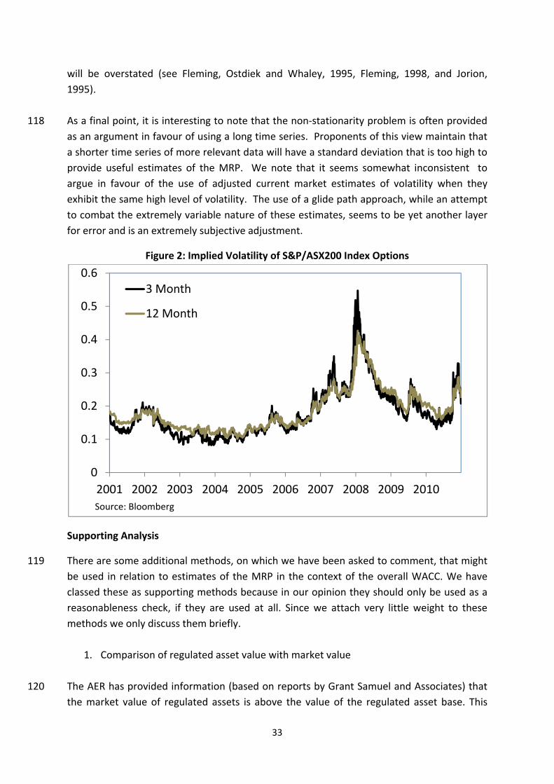
33

will be overstated (see Fleming, Ostdiek and Whaley, 1995, Fleming, 1998, and Jorion, 1995).

118 As a final point, it is interesting to note that the non-stationarity problem is often provided as an argument in favour of using a long time series. Proponents of this view maintain that a shorter time series of more relevant data will have a standard deviation that is too high to provide useful estimates of the MRP. We note that it seems somewhat inconsistent to argue in favour of the use of adjusted current market estimates of volatility when they exhibit the same high level of volatility. The use of a glide path approach, while an attempt to combat the extremely variable nature of these estimates, seems to be yet another layer for error and is an extremely subjective adjustment.

Figure 2: Implied Volatility of S&P/ASX200 Index Options

Supporting Analysis

119 There are some additional methods, on which we have been asked to comment, that might be used in relation to estimates of the MRP in the context of the overall WACC. We have classed these as supporting methods because in our opinion they should only be used as a reasonableness check, if they are used at all. Since we attach very little weight to these methods we only discuss them briefly.

1. Comparison of regulated asset value with market value

120 The AER has provided information (based on reports by Grant Samuel and Associates) that the market value of regulated assets is above the value of the regulated asset base. This

0

0.1

0.2

0.3

0.4

0.5

0.6

2001 2002 2003 2004 2005 2006 2007 2008 2009 2010

3 Month

12 Month

Source: Bloomberg

34

evidence is based on sales of regulated assets and prices for listed companies operating regulated networks. We have no evidence on how representative of regulated assets in general these sales and share prices are, but without exception they show market values above regulated values. The source of this value premium could arise from economies of scale and synergies in general, from the opportunities for efficiency gains, from opportunities for growth, from the potential to exploit tax shields, or because the allowed regulated return is above the return really required. It is difficult to attribute the value premium across these components. The premiums appear larger than the premiums that we would expect for the average takeover of about 30%, but the average takeover premium is a premium over market value and so is not directly comparable with a premium over regulated value. The evidence, however, provides no support for the proposition that a niggardly risk premium allowed by regulators is holding back the value of these regulated companies and makes them unattractive to investors.

2. lnformation from broker reports

121 The use of price and dividend/cash flow information from broker’s reports to infer future returns, takes us back to the discussion of the implied cost of capital where we argue that little weight should be given to this approach. In the discussion of the implied cost of capital we also mentioned the upward bias in analyst’s forecasts. This reinforces our view that we would give little weight to the implied future returns from broker’s reports.

122 It is well established that part of the bias in analysts’ forecasts is directly attributed to maintaining good relationships with the broker’s/investment bank’s corporate clients, for example, in supporting capital raisings and in the hope of continuing revenue from repeat business. For the same reasons that earnings forecasts may be biased, so the WACC’s in broker’s reports may also be biased and of course are subject to the same estimation problems and estimation errors as the WACC derived by the AER. Nonetheless, we do think that such estimates are of some interest and can be used as ball-park reasonableness check. Hence our inclusion, in the discussion of survey results, of MRPs obtained from independent expert reports by KPMG (2005) and Bishop (2009).

123 We do not wish to claim that broker’s reports are simply self-serving documents directed solely to the broker’s interests. It is clear, however, that such documents should be interpreted with the broker’s interests in mind. We suggest that while information from broker’s reports might be used as part of a reasonableness check, it should not be a primary basis for determining the MRP.

35

3. Comparison of the cost of debt and the cost of equity

124 Clearly the cost of equity has to be above the cost of company debt. The question is by how much? The key point is that given the problem we have measuring the market risk premium over risk free debt, we are likely have an even bigger problem measuring the risk premium over risky debt because we have additional sources of variation to deal with. Furthermore, severe credit/liquidity events like the GFC are likely to lead to instability in this premium.

125 The continuing use of the CAPM as the pre-eminent method to determine the cost of equity for companies suggests that there is no consensus on the magnitude for the premium of equity over company debt - otherwise companies would simply take their cost of debt and add the risk premium. We note however, that there are a substantial minority of companies who do this. The proportion of such firms is 47% according to Truong et. al. (2008) although other studies tend to report that less than 20% of firms use this method, for examples see Kester et. al.(1999) and Gitman and Vandenberg (2000). It is clear in the Truong et. al. study that there is overlap between the use of the CAPM and the debt plus equity premium method, so it appears there is some use as cross checks on each other.

126 The alternative is to turn to theory. Miller and Modigliani (1958) provide the basis for estimating the relationship between the cost of equity and leverage. The problem is that this reflects but one theory of capital structure. Several such theories exist however, and despite more than fifty years of debate, no consensus on the correct theory has emerged. Miller and Modigliani’s theory assumes that tax rates on debt and equity income are equal at the personal level. Miller (1977) relaxes this assumption and derives a different theory. Further modifications are required to take into account the effect of the Australian imputation system. Brealey, Myers, Partington and Robinson (2000) modify Miller’s theory to take into account imputation and present the following equation for the theoretical effect of debt on the value of the firm:

[ ] [ ]

−−−−+−−−

−+=)1(

)1)(1()1()1()1(1

p

GccpUL T

TTTTDVV

δγδ

127 Where VL is the value of the levered firm, Vu is the value of the unlevered firm, D is the

amount of debt, δ is the dividend payout ratio, Tp is the personal tax rate on dividends, Tc is

the corporate tax rate, TG is the tax rate on capital gains and γ measures the value of imputation tax credits recovered by investors as a proportion of the corporate tax paid.

128 We could possibly use this model as a basis to derive a relationship between the cost of equity and the cost of debt, but it is not worth the effort. Even if there were universal agreement that the above equation was the correct model,22 it contains several parameters

22 It is not the correct general model for Australia as it does not allow for partially franked dividends.

36

that have to be estimated. Unfortunately, it is an understatement to say that such estimates are likely to lack precision. In short, the theory of capital structure has a long, long way to go before it can be regarded as a remotely useful means of deriving equity risk premiums.

4. Cashflow analysis to meet credit rating metrics.

129 We have given limited consideration to this method, but we note the following. This approach uses key ratios, which are required to maintain a particular credit rating, as a means to derive cash flows and hence back out a cost of equity. As such, the previously discussed problems of the implied cost of capital apply with the addition of further problems relating to: the accuracy and stability of ratings; their consistency across rating agencies; their relation to financial ratios; and the stability of this relation over time. Work which uses financial ratios to partially explain credit ratings has been around since Pinches and Mingo (1973). However, such models have not replaced analysts because more than ratios determine ratings. We also expect that the relation between financial ratios and ratings will change over time. The rating process is not static, but is a dynamic process that depends both on the history of the company rating and changing conditions (see Dang and Partington, 2009). Consequently, we would give little weight to cash flow forecasts implied from ratings.

Conclusion

130 In this paper, we reviewed a number of different methods by which the equity market risk premium may be estimated. We broadly distinguish between four different methods: historical, utility, surveys and implied estimates, and find that each presents its own unique set of challenges and possesses its own limitations. As such, it is difficult to make an uncontested argument for the superiority of one method over another.

131 Of the four main methods that we review, the historical approach provides the traditional benchmark but such backward looking estimates require attenuation because of changes over time, survivorship bias and returns in excess of expectations. This appears to be a practice among utility regulators in the U.K. and is consistent with commonly cited academic sources such as Dimson, Marsh and Staunton (2002, 2003, 2008) and Welch (2000).

132 The utility method is not so much a process of estimation, as a theoretical framework to gauge the reasonableness of estimates derived from other methods. This framework suggests that historical risk premia are too high and may require downward adjustment.

133 While survey estimates suffer a number of problems, they do provide remarkably consistent evidence in support of a market risk premium of 6%. We would give this evidence some weight in an overall assessment of the premium.

37

134 In our opinion, there are many problems and subjective elements in implied (forward looking) market risk premium estimates from valuation models. These methods should therefore be used with great circumspection and restricted to a cross-check on the reasonableness of other methods.

135 In addition to the main methods, we also considered a number of alternative and supporting methods. Of these the adjusted global market risk premium appears to offer useful information worthy of some weight. The rest are at best used as reasonableness checks. There are many questions marks over the volatility based method, including the subjective nature of the ‘glide path’ adjustment. In relation to credit spreads, Bishop and Officer’s (2009) analysis of the change in the MRP consequent to increases in credit spreads is erroneous.

136 On balance, our view is that there is little compelling evidence to deviate from the long standing regulatory consensus of an equity market risk premium of 6%. If anything, the risk with this estimate is that it may prove to be an overstatement and it is possible to argue in favour of a downward adjustment.

38

References

Asher, A., (2011) “Equity Risk Premium Survey – Results and Comments” Actuary Australia, July, 13-14.

Bassanese, D. (2004) “Follow the money”, Australian Financial Review, 13 - 14 November.

Bishop, S. (2009) “IERs a Conservative and Consistent Approach to WACC Estimation by Valuers”, Value Advisor Associates.

Bishop, S. and Officer, B. (2009) “Market Risk Premium, Estimate for January 2010 – June 2014, Prepared for WestNet Energy”, Value Advisor Associates, December.

Bishop, S., Fitzsimmons, M. and Officer, B. (2011) “Adjusting the Market Risk Premium to Reflect the Global Financial Crisis”, JASSA, 1, 8 – 14.

Blume, M.E. (1974) “ Unbiased Estimators of Long-Run Expected Rates of Return”, Journal of the American Statistical Association, 69, 634-638.

Bodie, Z. (2002) “Longer Time Horizon Does Not Reduce Risk”, Financial Times, January 26.

Brailsford, T., Handley, J.C. and Maheswaran, K. (2008) “Re-examination of the historical equity risk premium in Australia”, Accounting and Finance, 48, 73–97.

Brealey, R.A., Myers, S.C., Partington, G. and Robinson, D. (2000) “Principles of Corporate Finance”, 1st Australian Edition, McGraw-Hill.

Brealey, R.A., Myers, S.C. and Allen, F. (2005) “Principles of Corporate Finance”, 8th Edition, McGraw-Hill/Irwin.

Bruner, R.F., Eades, K.M., Harris, R.S. and Higgins, R.C. (1998) “Best Practices in Estimating the Cost of Capital: Survey and Synthesis”, Finance Practice and Education, 8, 14–28.

Campbell, J. (2007) “Estimating the Equity Risk Premium”, Working Paper 13423, NBER Working Paper Series, September.

Carr, P. and Wu, L. (2003) “The Finite Moment Log Stable Process and Option Pricing”, Journal of Finance, 58, 753-777.

Claus, J. and Thomas, J. (2001) “Equity premia as low as three percent? Evidence from analysts’ forecasts for domestic and international stock markets”, Journal of Finance, 56,

1629–1666.

Cochrane, J.H. (1997) “Where is the market going? Uncertain facts and novel theories", Economic Perspectives, Federal Reserve Bank of Chicago, Nov, 3-37.

39

Cochrane, J.H. (2011) “Presidential Address: Discount Rates”, Journal of Finance, 66, 1047 – 1108.

Copeland, T., Koller, T. and Murrin, J. (2000) “Valuation: Measuring and Managing the Value of Companies”, (3rd ed), John Wiley & Sons, New York.

Damodoran, A. (2010) “A New “Risky” World Order: Unstable Risk Premiums Implications for Practice”, Working Paper, Stern School of Business.

Damodoran, A. (2011) “Equity Risk Premiums (ERP): Determinants, Estimation and Implications – The 2011 Edition”, Working Paper, Stern School of Business.

H. Dang and G. Partington (2009), “Rating Migrations: The Effect of History and Time”, Financial Management Association (European) Conference, Turin.

Dimson, E., Marsh, P. and Staunton, M. (2000) in Dimson, E., Marsh, P. and Staunton, M., “Risk and Return in the 20th and 21st Centuries,” Business Strategy Review Vol 11, 2 (2000

Dimson, E., Marsh, P., and Staunton, M. (2002) “Triumph of the Optimists: 101 years of global investment returns”, Princeton: Princeton University Press.

Dimson, E., Marsh, P. and Staunton, M. (2003) “Global Evidence on the Equity Risk Premium”, Journal of Applied Corporate Finance, 15, 27 - 38.

Dimson, E., Marsh, P. and Staunton, M. (2008) "The worldwide equity risk premium: a smaller puzzle." In: Mehra, R. (ed.) Handbook of the equity risk premium. Amsterdam: Elsevier.

Dimson, E., Marsh, P. and Staunton, M. (2011) “Credit Suisse Global Investment Returns Yearbook 2011”, Credit Suisse Research Institute, February.

Easton, P., (2006) “Use of Forecasts of Earnings to Estimate and Compare Cost of Capital Across Regimes" Journal of Business, Finance and Accounting, 33, 374-394.

Easton, P.D. and Sommers, G.A. (2006) “Bias in Expected Rates of Return Implied by Analysts’ Earnings Forecasts”, Working Paper.

Fama, E.F. and French, K.R. (1988) “Dividend yields and expected stock returns”, Journal of Financial Economics, 22, 3–25.

Fernandez, P. (2006) “Equity Premium: Historical, Expected, Required and Implied”, IESE Business School Working paper.

Fernandez, P. (2009) “The Equity Premium in 150 Textbooks”, IESE Business School, Working Paper.

40

Fernandez, P. (2011) “Market Risk Premium used in 56 countries in 2011: A survey with 6,014 answers”, IESE Business School, Working Paper.

Fisher, K.L. and Statman, M. (2000) “Investor Sentiment and Stock Returns”, Financial Analysts Journal, 56, 16-23.

Fisher, K.L. and Statman, M. (2000a) “Cognitive Biases in Market Forecasts”, The Journal of Portfolio Management, Fall, 72-81.

Fisher, K.L. and Statman, M. (2003) “Consumer Confidence and Stock Returns”, The Journal of Portfolio Management, Fall, 2003.

Fleming, J., Ostdiek, B. and Whaley, R.E. (1995) “Predicting stock market volatility: A new measure”, Journal of Futures Markets, 15, 265–302.

Fleming, J. (1998) “The quality of market volatility forecasts implied by S&P 100 index option prices”, Journal of Empirical Finance, 5, 317 - 345.

Gailbraith, J.K. (1993) “A Short History of Financial Euphoria”, Penguin Books, London, England.

Gitman, L. and Vandenberg, P. 2000, “Cost of capital techniques used by major U.S. firms: 1997 vs. 1980”, Financial Practice and Education, 10, 53-68.

Goetzmann, W. and Ibbotson, R. (2005) “History and the Equity Risk Premium”, Yale ICF Working Paper No. 05-04, April.

Goyal, A. and Welch, I. (2003) “Predicting the Equity Premium with Dividend Ratios”, Management Science, 49, 639–654.

Graham, J.R. and Harvey, C.R. (2010) “The Equity Risk Premium in 2010”, Working Paper.

S Gray (2001), “Issues in Cost of Capital Estimation”, Working Paper

Gray S. and Officer R. (2005) “A Review of the Market Risk Premium and Commentary on Two Recent Papers, A Report Prepared for the Energy Networks Association”, Report.

Hancock, (2005) “The Market Risk Premium for Australian Regulatory Decisions: Preliminary Report”, The South Australian Centre for Economic Studies, April.

Handley (2011) “An Estimate of the Historical Equity Risk Premium for the Period 1883 to 2010” Report prepared for the AER.

Hathaway, N. (2005) “Australian Market Risk Premium”, Capital Research Pty Ltd.

Headberry Partners P/L and Bob Lim & Co P/L (2003) “Further capital markets evidence in relation to the market risk premium and equity beta values”, December.

41

Heaton, J. and Lucas, D. (1999) “Stock Prices and Fundamentals”, NBER Macroeconomics Annual, 14, 213-242.

Indro, D.C. and Lee, W.Y. (1997) “Biases in arithmetic and geometric averages as estimates

of long-run expected returns and risk premia”, Financial Management, 26, 81–90.

Jorion, P. (1995) “Predicting volatility in the foreign exchange market”, Journal of Finance, 50, 507–528.

Jorion P. and Goetzmann W. (1999) “Global Stock Markets in the Twentieth Century,” Journal of Finance, 54, 953-980 .

Kester, G., Chang, R., Echanis, E., Haikal, S., Isa, M., Skully, M., Kai-Chong, T. & Chi-Jeng, W. 1999, “Capital budgeting practices in the Asia-Pacific Region: Australia, Hong Kong, Indonesia, Malaysia, Philippines, and Singapore”, Financial Practice and Education, 9, 25-33.

Kostin, D.J. (2011) “Where to Invest Now: Rising Profits Despite a Faltering Economy”, Goldman Sachs Research Report.

KPMG (2005) “Cost of Capital – Market practice in relation to imputation credits; Victorian Electricity Distribution Price Review 2006-10”, Report.

Lally, M. (2005) “Structural Breaks and the Estimation of the Market Risk Premium in Australia”, Report prepared for the Queensland Competition Authority, April 15.

Lonergan, W. (2001) “The Disappearing Returns: Why Imputation Has Not Reduced the Cost of Capital”, JASSA, 1, 8–17.

Merton, R.C. (1980) “On estimating the expected return on the market”, Journal of Financial Economics, 8, 323-361.

Mehra, R. and Prescott, E.C. (1985) “The equity premium: A puzzle”, Journal of Monetary

Economics, 15, 145–161.

Miller, M. and Modigliani, F. (1958) “The Cost of Capital, Corporation Finance and the Theory of Investment” 48, 261-297

Miller M., (1977) “Debt and Taxes”, Journal of Finance, 32, 261–76

Officer, R.R. (1989) “Rates of Return to Shares, Bond Yields and Inflation Rates: An Historical Perspective” in Ball, R. et al (eds) Share Markets and Portfolio Theory, 2nd Ed., University of Queensland Press.

Officer, R. and Bishop, S. (2008) “Market Risk Premium a Review Paper”, Value Advisor Associates, August.

42

Pinches, G. and Mingo, K., (1973) “A Multivariate Analysis of Industrial Bond Ratings” Journal

of Finance, 1-18.

Reitz, T. (1988) “The Equity Premium: A Solution?”, Journal of Monetary Economics, 22, 133–136.

Santa-Clara, P. and Yan, S. (2006) “Crashes, Volatility, and the Equity Premium: Lessons from S&P 500 Options”, Review of Economics and Statistics, 92, 435-451.

Scherbina, A. (2004) “Analyst Disagreement, Forecast Bias and Stock Returns”, Working Paper.

Siegel, J.J. (1999) “The Shrinking Equity Premium”, Journal of Portfolio Management, 26, 10 – 17.

Siegel, J.J. and Thaler, R.H. (1997) “Anomalies: The Equity Premium Puzzle”, The Journal of Economic Perspectives, 11, 191-200.

Truong, G. and Partington, G. (2007), “Alternative Estimates of the Cost of Equity Capital for Australian Firms”, 20th Australasian Finance and Banking Conference, Sydney.

Truong, G., Partington, G. and Peat, M. (2008) “Cost of Capital Estimation and Capital Budgeting Practice in Australia”, Australian Journal of Management, 33, 95 – 121.

Welch, I. (2000) “Research Roundtable The Equity Premium”, Working Paper, June 30.

Welch, I. (2000a) “Views of Financial Economists on the Equity Premium and on Professional Controversies”, Working Paper,

Welch, I. (2001) “The Equity Premium Consensus Forecast Revisited”, Working Paper, Yale School of Management, September.

Welch, I. (2008) “The Consensus Estimate for the Equity Premium by Academic Financial Economists in December 2007”, Working Paper, January.

43

Appendix A : Resumes

Professor Michael Mckenzie

Chair of the Discipline of Finance

Faculty of Economics and Business

The University of Sydney

Contact Details :

Address: Discipline of Finance

Economics and Business Building (H69),

University of Sydney

New South Wales, 2006.

Telephone: + 61 (0)2 9114 0578

Fax: + 61 (0)2 9351 6461

Email: michael.mckenzie@sydney.edu.au

Qualifications :

B.B.S. (Economics) - Massey University (New Zealand)

M.Ec. (Economics) - Monash University (Australia)

Ph.D. (Finance) - RMIT University (Australia)

PROFESSIONAL

44

Professor McKenzie worked as a Treasury Analyst for the Australian Treasury Group at Deloitte Touche Tohmatsu before leaving to complete his PhD at RMIT in 1995.

In 1997, Professor McKenzie became an associate of the Midwine Consulting, which is a Sydney based company that specialises in financial risk management consulting and business process re-engineering. This appointment is current and ongoing.

ACADEMIC

Dr. Michael McKenzie is a Professor of Finance and also the Chair of Discipline of Finance in the Faculty of Economics and Business at The University of Sydney (Australia) and a Research Associate at the Centre for Financial Analysis and Policy (CFAP), Cambridge University (UK).

Professor McKenzie has published numerous books and journal articles on a wide range of topics. His main research interests, encompass the areas of corporate finance, risk management, market volatility, price discovery and market microstructure analysis.

BOOKS / MONOGRAPHS

1. McKenzie, M and Brooks, R. (1998) “ARCH Modelling of Financial Market Volatility” Volume 2 in the McGraw-Hill Series in Advanced Corporate Finance, McGraw-Hill.

2. Kim, S-J. and McKenzie, M.D. (2008) International Financial Review, Volume 8 : Asia-Pacific Financial Markets: Integration, Innovation and Challenges, Elsevier Publishing Company, UK.

3. Kim, S-J and McKenzie, M.D. (Eds.) (2010) International Financial Review, Volume 11 : International banking in the new era: Post crisis challenges and opportunities, Emerald, U.K., Forthcoming in Dec.

PUBLISHED PAPERS / BOOK CHAPTERS

1. Mckenzie, M.D. (1997) “ARCH Modelling of Australian Bilateral Exchange Rate Data” Applied Financial Economics (7) pp. 147 - 164.

45

2. Brooks, R.D., Faff, R.W. and Mckenzie, M.D. (1997) “Bivariate GARCH Estimation of Beta Risk in the Australian Banking Industry” Accountability and Performance: Special Issue on the Wallis Enquiry, 3, pp. 81 - 102.

3. Mckenzie, M.D. and Brooks, R.D. (1997) “The Impact of Exchange Rate Volatility on US-German Trade Flows” Journal of International Financial Markets, Institutions and Money (7) pp. 73 - 87.

4. Brooks, R.D., Faff, R.W. and Mckenzie, M.D. (1998) “Time Varying Beta Risk of Australian Industry Portfolios : A comparison of modelling techniques” Australian Journal of Management, 23, pp. 1 - 22.

5. Mckenzie, M.D. (1998) “The Impact of Exchange Rate Volatility on Australian Trade Flows” Journal of International Financial Markets, Institutions and Money (8) pp. 21 - 38.

6. Mckenzie, M.D. (1999) “Power Transformation and Forecasting the Magnitude of Exchange Rate Changes” International Journal of Forecasting (15) pp. 49 - 55.

7. Mckenzie, M.D. (1999) “The Impact of exchange rate volatility on International Trade Flows” Journal of Economic Surveys (13) pp. 71 - 106 .

8. Stewart, M.F., Shannon, J.S., and McKenzie, M.D. (1999) “A Variable Rate Goods and Services Tax (GST) for Australia?” Economic Papers (18) pp. 78 - 94.

9. McKenzie, M.D. (1999) “Risk in the Japanese Banking Sector : Implications of the Financial Systems Reform Act (1992)” The Asia-Pacific Journal of Economics and Business (3) pp. 4 - 20.

10. Brooks, R.D., Faff, R.W., Ho, Y.K. and Mckenzie, M.D. (2000) “U.S. Banking Sector Risk in an Era of Regulatory Change : A bivariate GARCH approach” Review of Quantitative Finance and Accounting (14) pp. 17 – 44.

11. Brooks, R.D., Faff, R.W., McKenzie, M.D. and Mitchell, H. (2000) “A Multi-country Study of Power ARCH Models and National Stock Market Returns” Journal of International Money and Finance, 19, pp. 377 - 397.

12. Brooks, R.D., Faff, R.W., Ho, Y.K. and McKenzie, M.D. (2000) “Exploring the Economic Rationale of Extremes in GARCH Generated Betas : The case of US Banks” Quarterly Review of Economics and Finance, 40, 85 – 106.

13. Mckenzie, M.D., Brooks, R.D., and Faff, R.W. (2000) “The Use of Domestic and World Market Indexes in the Estimation of Time-Varying Betas” Journal of Multinational Financial Management, 10, pp. 91 – 106.

46

14. McKenzie, M.D., Mitchell, H., Brooks, R.D. and Faff, R.W. (2001) “Power ARCH Modelling of Commodity Futures Data on the London Metals Exchange” European Journal of Finance, 7, pp. 22 - 38.

15. McKenzie, M.D. (2001) “Chaotic Behaviour in National Stock Market Indices : New Evidence from the Close Returns Test” Global Finance Journal, 12, pp. 35 – 53.

16. McKenzie, M.D., Brailsford, T.J. and Faff, R.W. (2001) “New Insights into the Impact of the Introduction of Future Trading on Stock Price Volatility” Journal of Futures Markets (21) pp. 237–255

17. McKenzie, M.D. (2001) “Non-periodic Australian Stock Market Cycles: Evidence from Rescaled Range Analysis” The Economic Record, 77, 393 – 406.

18. McKenzie, M.D. and Faff, R.W. (2002) “The Impact of Stock Index Futures Trading on Daily Returns Seasonality : A Multicountry Study” Journal of Business (Jan) Vol. 75 (1) 95 - 125.

19. Frino, A. and McKenzie, M.D. (2002) “The Pricing of Stock Index Futures Spreads at Contract Expiration” Journal of Futures Markets (22) pp. 451-469

20. McKenzie, M.D. and Mitchell, H. (2002) “Generalised Asymmetric Power ARCH Modeling of Exchange Rate Volatility” Applied Financial Economics, 12, 555 - 64.

21. Brooks, R.D., Faff, R.W. and Mckenzie, M.D. (2002) “Time Varying Country Risk : An assessment of alternative modelling techniques” The European Journal of Finance, 8, pp. 249 - 274.

22. McKenzie, M.D. (2002) “The Economics of Exchange Rate Volatility Asymmetry” International

Journal of Finance and Economics, 7, 247 - 60.

23. McKenzie, M.D. and Brooks, R.D. (2003) “The Role of Information in Hong Kong Individual Stock Futures Trading” Applied Financial Economics, 13, 123 – 131.

24. McKenzie, M.D. and Faff, R.W. (2003) “The Determinants of Conditional Autocorrelation in Stock Returns” The Journal of Financial Research, 26, 259 - 274.

25. McKenzie, M.D. and Frino, A. (2003) “The tick/volatility ratio as a determinant of the compass rose: Empirical evidence from decimalisation on the NYSE” Accounting and Finance, 43, 331 - 44.

47

26. Mitchell, H. and McKenzie, M.D. (2003) “GARCH Model Selection Criteria” Quantitative Finance, 3, 262 – 84.

27. Frino, A. and McKenzie, M.D. (2003) “The Impact of Screen Trading on the Link Between Stock Index and Stock Index Futures Prices: Evidence from UK Markets” Proceedings of the IASTED International Conference on Financial Engineering and Applications, Ed. Hamza, M.H., The International Association of Science and Technology for Development, 103 - 112.

28. Faff, R.W., Hallahan, T. and McKenzie, M.D. (2003) “An Exploratory Investigation of the Relation between Risk Tolerance Scores and Demographic Characteristics” Journal of Multinational Financial Management, 13, 483-502.

29. Kim, S-J., McKenzie, M.D. and Faff, R.W. (2004) “Macroeconomic News Announcements and the Role of Expectations: Evidence for US Bond, Stock and Foreign Exchange Markets” Journal of Multinational Financial Management (14,3) pp. 217 - 232.

30. McKenzie, M.D. (2004) “An Empirical Examination of the Relationship Between Central Bank Intervention and Exchange Rate Volatility: Some Australian Evidence” Australian Economic Papers, 43, 59 – 74.

31. Faff, R.W., Hallahan, T. and McKenzie, M.D. (2004) “An Empirical Investigation of Personal Financial Risk Tolerance” Financial Services Review, 13(1), 57 - 79.

32. McKenzie, M.D. (2004) “The Effects of Exchange Rate Volatility on Trade” Chapter 8 in De Brower, G. and Kawai, M. Eds. “Exchange Rate Regimes in East Asia” Routledge Curzon Studies in the Growth Economies of Asia, Routledge Curzon Publishing Co., London.

33. Mitchell, H. and McKenzie, M.D. (2004) “The Use of Forecasting Accuracy as an ARCH Model Selection Tool” Modelling and Analysis of Safety and Risk in Complex Systems, Russian Academy of Sciences, International Scientific School, June, 111 - 117.

34. Mckenzie, M.D. (2004) “The Relationship Between Market Size, Concentration and Stock Index Autocorrelation” Finance Letters, 2(5), pp ? - ?.

35. McKenzie, M.D. and Faff, R.W. (2005) “Modelling Conditional Return Autocorrelation” International Review of Financial Analysis, 14, 23 - 42.

36. Faff, R.F., Hillier, D. and McKenzie, M.D. (2005) “An Investigation of Autocorrelation and Cross

Autocorrelation in Emerging Markets” Review of Pacific Basin Financial Markets and Policies, 8, 467 – 499.

48

37. Henry, O. and Mckenzie, M.D. (2006) “The Impact of Short Selling on the Price–Volume Relationship: Evidence from Hong Kong” Journal of Business, 79, 671 - 692.

38. Cai, C.X., Faff, R.W., Hillier, D.J. and McKenzie, M.D. (2006) “Modelling Return and Conditional Volatility Exposures in Global Stock Markets” Review of Quantitative Finance and Accounting, 27, 125 – 42.

39. Mitchell, H. and Mckenzie, M.D. (2006) “A Note on the Wang and Wang Measure of the Quality of the Compass Rose” Journal of Banking and Finance, 30, 3519 - 24.

40. McKenzie, M.D. and Kim, S.J. (2007) “Evidence of an Asymmetry in the Relationship Between Volatility and Autocorrelation” International Review of Financial Analysis, 16, 22-40.

41. Mckenzie, M.D. (2007) “Technical Trading Rules in Emerging Markets and the 1997 Asian Currency Crises” Emerging Markets Finance and Trade, 43 (4), 46 - 73.

42. Heaney, R., Naughton, T., Fry, T., Davidson S. and McKenzie M.D. (2007) “The Link Between Performance and Changes in the Size and Stability of a Firm's Officers and Directors” Journal of Multinational Financial Management, 17, 16-29.

43. Faff, R.W., and McKenzie, M.D. (2007) “The Relationship Between Implied Volatility and Autocorrelation for US Stock Market Indices” International Journal of Managerial Finance, 3, 191 – 196.

44. Mckenzie, M.D. (2007) “International Evidence on the Determinants of the Decision to List” Australian Journal of Management,32 (1), 2007, 1 - 28.

45. Kim, S.J. and McKenzie, M.D. (2008) “Conditional Autocorrelation and the Integration of Stock Markets” Ch. 4 in Kim, S.J. and McKenzie, M.D. Eds. International Financial Review, Volume 8 : Asia-Pacific Financial Markets: Integration, Innovation and Challenges, Elsevier, UK.

46. Mitchell, H. and McKenzie, M.D. (2008) “A comparison of alternative techniques for selecting an optimum ARCH model” Journal of Statistical Computation and Simulation, 78, 51 – 67.

47. McKenzie M (2008) “Equity Arbitrage” in Trade Execution, Arbitrage and Dealing in Australia, ed. A Frino and R Segara, Pearson Education, Sydney, Australia pp. 67-97.

48. Faff, R.W., Hillier, D. and McKenzie, M.D. (2008) “Modelling Return and Volatility Exposures in the Global Stock Markets” Forthcoming in Global Finance Journal.

49

49. Dungey, M., McKenzie, M.D. and Tambakis, D. (2008) “The Flight-to-Quality and Asymmetric Volatility Responses in US Treasuries” forthcoming Global Finance Journal (19).

50. Faff, R.W., Hallahan, T. and McKenzie, M.D. (2008) “Non-linear Linkages between Financial Risk Tolerance and Demographic Characteristics” Forthcoming in Applied Economics Letters

51. Sadorsky, P. and Mckenzie, M.D. (2008) “Power Transformation Models and Volatility Forecasting” Forthcoming in the Journal of Forecasting.

52. Dungey, M., Frino, A. and Mckenzie, M.D. (2008) “Public Information, Price Volatility and Trading Volume in US Bond Markets” Forthcoming in Review of Futures Markets.

53. Dungey, M., Mckenzie, M.D. and Smith, V. (2009) “Empirical Evidence on Jumps in the Term Structure of the US Treasury Market” Journal of Empirical Finance, 16 (3), 430-445.

54. Faff, R.W., Hallahan, T. and McKenzie, M.D. (2009) “Non-linear Linkages between Financial Risk Tolerance and Demographic Characteristics”, Applied Economics Letters, 16, 1329 – 1332.

55. Daniel Schmidt, Daniel Spring, Ralph MacNally, James R. Thomson, Barry W. Brook, Oscar Cacho, Michael McKenzie (2010) "Finding needles (or ants) in haystacks: Bayesian prediction of locations of invasive organisms to inform eradication and containment programs" Forthcoming in Ecological Applications.

56. Daniel Spring, Jiri Baum, Michael D. McKenzie, Ralph MacNally, A. Sanchez-Azofeifa, James Thomson (2009) “Building a Regionally Connected Reserve Network in a Changing and Uncertain World” Forthcoming in Conservation Biology

50

RESEARCH AWARDS

Recipient of the E. Yetton Award for paper of the year by the Editors of the Australian Journal of Management for the paper “Time-Varying Beta Risk of Australian Industry Portfolios: A comparison of modelling techniques”, 1998.

Runner-up for the E. Yetton Award for paper of the year by the Editors of the Australian Journal of Management for the paper “International Evidence on the Determinants of the Decision to List”, 2007.

51

A S S O C I A T E P R O F E S S O R G R A H A M PA R T I N G T O N

CURRICULUM VITAE FACULTY OF ECONOMICS AND BUSINESS UNIVERSITY OF

SYDNEY

PERSONAL Name: Associate Professor Graham Harold PARTINGTON

Academic Qualifications:

B.Sc. (Hons) Economics/Forestry, University of Wales, 1971

MEc. (Hons), by thesis, Macquarie University, 1983.

Awards 1985: Butterworths Travelling Fellowship

2000: Peter Brownell Manuscript Award. Awarded by the Accounting Association of Australia and New Zealand for the best paper in Accounting and Finance, 1999

2001: Manuscript award for the best paper: Education Notes, Accounting Research Journal, 2000.

2009 Bangor University Senate conferred the title: Honorary Visiting Senior Research Fellow (2009-2012.)

2009 Chartered Financial Analyst (CFA) best paper prize (Asian Investments) at the Asian Finance Association Conference.

Address: Economics and Business Building (H69),

Finance Discipline

University of Sydney

NSW 2006

Telephone: 61 (0)2 9036-9429

Fax: 61 (0)2 9351-6461

Email: G.Partington@econ.usyd.edu.au

52

Current position University of Sydney Faculty of Economics and Business

Sept 2002–to date: Associate Professor, Finance Discipline (Head of Postgraduate Research 2002-2007, 2009 to date)

Education Director Capital Markets Co-operative Research Centre 2002-2008

PUBLICATIONS

Books Brealey, R., S. Myers, G. Partington and D. Robinson, Principles of Corporate Finance, Australian Edition, McGraw-Hill 2000 (1st printing 2000, 2nd printing 2000.)

C.A. Martin, J. McKinnon, R. Hines, G. Harrison and G. Partington, An Introduction to Accounting, McGraw-Hill (1st edition, 1983, 2nd edition, 1988, 3rd edition 1990.)

Contributions and Chapters in Books G. Partington, Valuation and Project Selection when the Market and Face Value of Dividends Differ, in Qfinance the Ultimate Resource, Bloomsbury Press, 2009.

G. Partington, Dividend Imputation Credits and Valuation, in Business Tax Reform, Australian Tax Research Foundation, 2007.

R. J. Coombes, M. Craig-Lees, M. McGrath, P. O'Sullivan, G. Partington and J. M. Wood, Business Studies Book Two, Social Science Press 1991.

R. J. Coombes, M. Craig-Lees, M. McGrath, P. O'Sullivan, G. Partington and J. M. Wood, Business Studies Book One, Social Science Press 1990.

E. Carew, The Language of Money, George Allen and Unwin, 1985.

Refereed Journals

PUBLISHED

G. Partington, Discussion of an International Analysis of Dividend Payment Behaviour, Journal of Business Finance and Accounting., 36:3-4, 2009, pp. 523-529.

G. Truong, G. Partington and M. Peat, Cost of Capital Estimation and Capital Budgeting Practice in Australia, Australian Journal of Management, 33:1, 2008, pp. 95- 122.

M. Dempsy and G. Partington, The Cost of Capital Equations under the Australian Imputation Tax System, Accounting and Finance, 48:3, 2008, pp. 439-460.

53

H. Chu and G. Partington, The Market Valuation of Cash Dividends: The Case of the CRA Bonus Issue, International Review of Finance, 2008, 8:1-2, pp. 1-20,

L. Hodgkinson and G. Partington, The Motivation for Takeovers in the UK, Journal of Business Finance and Accounting, Vol. 35, Issue 1-2,2008, pp. 102-126

A. Jun, V. Alaganar, G. Partington and M. Stevenson, Price and Volume Behaviour around the Ex-dividend Day: Evidence on the Value of Dividends from ADRs and their Underlying Australian Stocks,2008 International Review of Finance, 8:1-2, 2008, pp. 21-55,

G. Truong and G. Partington, The Relation between Franking Credits and the Market Risk Premium: A Comment, Accounting and Finance, 48:1, 2008, pp. 153-158.

B. Wong, G. Partington, M. Stevenson and V. Torbey, Surviving Chapter 11 Bankruptcies: Duration and Payoff? Abacus, 43:1, 2007, pp.363-387.

G. Partington, Discussion of Dargenidou, Mcleay and Raonic (Expected Earnings Growth and the Cost of Capital: An Analysis of Accounting Regime Change in the European Financial Market) Abacus 42:3-4, 2006, pp. 415-425.

S. Armitage, L. Hodgkinson and G. Partington, The Market Value of UK Dividends from Shares with Differing Entitlements, Journal of Business Finance and Accounting, 33:1, 2006, pp 150-174.

G. Partington, M Stevenson and J. Yao, Run length and the Predictability of Stock Price Reversals. Accounting and Finance, 45: 4, 2005, pp. 653-671,

G. Partington, P Russell, M. Stevenson and V. Torbey, Predicting Return Outcomes for the Shareholders of Companies Entering Chapter 11 Bankruptcy, Managerial Finance, 27:5, 2001.

G. Partington and M. Stevenson, The Probability and Timing of Price Reversals in the Property Market, Managerial and Decision Economics, 22:7, 2001, pp.389-398.

H. Chu and G. Partington, Dangers in Data Adjustment: The Case of Rights Issues and Returns, Accounting and Finance, 41:2, 2001, pp.143-168.

G. Partington and S. Walker, A Note on Transactions Costs and the Interpretation of Dividend Drop-off Ratios, Accounting and Finance, 41:2, 2001, pp. 229-241.

S. Walker and G. Partington, A Market Valuation for Optus Pre-listing: A Case Note, Accounting Research Journal, 13:2, 2000, pp. 90-94. (This paper won the award for Best Paper: Education Notes.)

S. Walker and G. Partington, The Value of Dividends: Evidence from Cum-dividend Trading in the Ex-dividend Period, Accounting and Finance, 39:3, 1999, pp. 275-296. (This paper won the Peter Brownell Manuscript Award).

G. Hobbes, G. Partington and M. Stevenson, Earnings Dividends and Returns: A Theoretical Model, Research in Finance, Summer 1996, pp. 221-244.

G. Partington, Variables Influencing Dividend Policy in Australia: Survey Results, Journal of Business Finance and Accounting 16:2, 1989, pp.165-182.

C.A. Martin, J. L. McKinnon and G. Partington, Funds Statements and the Two Entity Test: A Response, Abacus, 22:1, 1986, pp. 39-44.

54

G. Partington, Dividend Policy and its Relationship to Investment and Financing Policies: Empirical Evidence, Journal of Business Finance and Accounting, 12:4, 1985, pp. 531-542.

G. Partington, Dividend Policy and Target Payout Ratios, Accounting and Finance, 24:2, 1984, pp. 63-74.

G. Partington, Teaching Process Costing, Issues in Accounting Education, 2, 1984, pp. 75-90.

C.A. Martin, J. L. McKinnon and G. Partington, Clarifying Funds Statements: The Two Entity Test Accounting and Finance, 23:1, 1983, pp. 79-87.

R. H. Chenhall and G. Partington, Dividends Distortion and Double Taxation, Abacus, 19:1, 1983, pp. 3-13.

G. Partington, Financial Decisions the Cost(s) of Capital and the Capital Asset Pricing Model, Journal of Business Finance and Accounting, 8:1, 1981, pp. 97-112.

G. Partington, Process Costing: A Comment, 15:1, Abacus, June 1979, pp.60-66.

G. Partington, The Tax Deductibility of Interest Payments and the Weighted Average Cost of Capital: A Comment, Journal of Business Finance and Accounting, 6:1, 1979, pp.95-100.

Revise and resubmit A. Jun, D. Gallagher and G. Partington, An Examination of Institutional Dividend Clienteles: Evidence from Australian Institutional Portfolio Holdings, Journal of Business Finance and Accounting, 2008.

Andrew B. Ainsworth, Kingsley Fong, David R. Gallagher, Graham Partington, Institutional Trading Around the Ex-Dividend Day, Journal of Financial Economics, 2008

H. Chu and G. Partington, The Value of Dividends: Evidence from a New Method, Journal of Finance, 2003

Conference Papers Andrew B. Ainsworth, Kingsley Fong, David R. Gallagher, Graham Partington, Institutional Trading Around the Ex-Dividend Day, Asian Finance Association Conference, Brisbane, 2009. Winner of the CFA best paper prize (Asian Investments.)

H. Dang and G. Partington, Rating Migrations: The Effect of History and Time, European Financial Management Association Annual Meeting, Athens, 2008.

H. Dang and G. Partington, Rating History and the Rating Dynamics of Fallen Angels, Rising Stars, and Big Rating Jumpers, Risk Management Conference: Credit and Financial Risk Management 40 Years after the Altman Z-score Model, Florence, 2008.

55

Juan Yao, Graham Partington, Max Stevenson, Predicting the Directional Change in Consumer Sentiment, The 28th Annual Symposium on Forecasting, Nice 2008.

Maria Kim and Graham Partington, The Dynamic Prediction of Corporate Failure, Australasian Finance and Banking Conference, 2008.

M. Dempsey and G. Partington, Cost of Capital and Valuation Equations that Work for Any Tax System: Their Application under the Australian Imputation Tax System, Multinational Finance Association Conference, Thessalonica, 2007.

H. Dang and G. Partington, Modeling Rating Migrations, Poster Session, CREDIT 2007 Conference, Venice 2007

G. Truong and G. Partington, Alternative Estimates of the Cost of Equity Capital for Australian Firms, 20th Australasian Finance and Banking Conference, Sydney, 2007

G. Partington, Dividend Imputation Credits and Valuation, Business Tax Reform Meet the Critics, Australian Tax Research Foundation Conference, Sydney, 2006. G. Truong and G. Partington, The Value of Imputation Tax Credits and Their Impact on the Cost of Capital, Accounting and Finance Association of Australia and New Zealand Conference, Wellington, 2006. A. Jun, D. Gallagher and G. Partington, An Examination of Institutional Dividend Clienteles: Evidence from Australian Institutional Portfolio Holdings, Accounting and Finance Association of Australia and New Zealand Conference, Wellington, 2006. Jun, A. and Partington G., Taxes International Clienteles and the Value of ADR Dividends, Multinational Finance Association Conference, Edinburgh, 2006.

G. Partington and Stevenson S, A Distress Prediction Tool, New Directions in Employment and Financial Security: Rethinking Employee Entitlements and Employee Buyouts. Workplace Relations Centre and Members Equity Workshop, 2006, Sydney.

H. Chu and G. Partington, The Market Valuation of Cash Dividends: The Case of the CRA Bonus Issue, The European Financial Management Association Annual Meeting, Milan, 2005.

56

G. Truong, G. Partington and M. Peat, Cost of Capital Estimation and Capital Budgeting Practice in Australia, Accounting and Finance Association of Australia and New Zealand Conference, Melbourne, 2005. A. McAdam, and G. Partington, Does the Choice of Share Price Matter when Examining Takeovers? Accounting and Finance Association of Australia and New Zealand Conference, Melbourne, 2005.

A. Jun, , V. Alaganar, G. Partington and M. Stevenson, Price and Volume Behaviour around the Ex-dividend Day: Evidence on the Value of Dividends from ADRs and their Underlying Australian Stocks, Accounting and Finance Association of Australia and New Zealand Conference, Alice Springs, 2004. M. Dempsey and G. Partington, The Cost of Capital Equations Under the Australian Imputation Tax System, Accounting Association of Australia and New Zealand Conference, Alice Springs, 2004. S. Armitage, L. Hodgkinson and G. Partington, The Value of Dividends to a Marginal Investor, Evidence using Contemporaneous Trading Data, British Accounting Association Conference, Jersey, 2002. H. Chu and G. Partington, The Value of Dividends: Evidence from a New Method, Accounting Association of Australia and New Zealand Conference, Auckland 2001. G. Partington, P Russell, M. Stevenson and V. Torbey, Predicting Return Outcomes for the Shareholders of Companies Entering Chapter 11 Bankruptcy, Accounting Association of Australia and New Zealand Conference, Auckland 2001. H. Chu, L. Hodgkinson and G. Partington, Right’s Trade Adjustments: Evidence from the UK, British Accounting Association Conference, Nottingham 2001 H. Chu and G. Partington, The Value of Dividends Implicit in Rights Prices, Australasian Finance and Banking Conference Sydney, 2001.

L. Hodgkinson and G. Partington, The Motivation for Takeovers in the UK, British Accounting Association Conference, Exeter, 2000. V. Alaganar, G. Partington and M. Stevenson, Do Ex-dividend Drop-offs Differ Across Markets? Evidence From Internationally Traded (ADR) Stocks, Accounting Association of Australia and New Zealand Conference, Hamilton Island, 2000. G. Partington and S. Walker, A Theory of Ex-Dividend Equilibrium Under Imputation and Some Empirical Results, Accounting Association of Australia and New Zealand Conference, Hamilton Island, 2000.

57

G Partington and S. Walker, The 45-Day Rule: The Pricing of Dividends and the Crackdown on Trading in Imputation Credits, Accounting Association of Australia and New Zealand Conference, Cairns, 1999.

S. Walker and G. Partington, Optus: A Market Valuation Pre-listing, Accounting Association of Australia and New Zealand Conference, Cairns, 1999.

H. Chu and G. Partington, Dangers in Data Adjustment: The Case of Rights Issues, Australasian Finance and Banking Conference, Sydney, 1999.

G. Hobbes, G. Partington and M.J. Stevenson, A General Model of Earnings Dividends and Returns, Australasian Finance and Banking Conference, University New South Wales, Sydney, 1997

S. Walker and G. Partington, The Ex-Dividend Drop-off: Evidence from Cum-dividend Trading in the Ex-dividend Period, Accounting Association of Australia and New Zealand Conference, Hobart, 1997.

G. Hobbes, G. Partington and M.J. Stevenson, Earnings Dividends and Returns: A Theoretical Model, Asia-Pacific Finance Association Conference, Hong Kong, 1995.

G. Partington and E. Hutson, Share Prices, Takeover Outcomes and the Expected Value Hypothesis, invited paper at the University of Wales Accounting Colloquium, Gegynog, 1994.

G. Partington and E. Hutson, Share Prices, Takeover Outcome sand the Volume of Trades, Australasian Finance and Banking Conference, Sydney, 1994

G. Partington, M. Peat and M. Stevenson, The Probability and Timing of Corporate Financial Distress: Preliminary Results for Australia, Australasian Finance and Banking Conference, Sydney, 1992.

G. Partington, M. Peat and M. Stevenson, Estimating the Probability and Timing of Financial Distress, Australian Institute of Bankers Conference, Melbourne 1991.

58

P. Eddey, G. Partington and M. Stevenson, Predicting the Probability and Timing of Takeover Success, Australasian Finance and Banking Conference, Sydney, 1989.

G. Partington and T. Valentine Finance for Australian Industry, Metal Trades Industry Conference, Sydney 1984.

G. Partington, Why Firms Use Payout Targets: A Comparative Study of Dividend Policy, Accounting Association of Australia and New Zealand Conference, Brisbane, 1983.

Unpublished Working Papers H. Chu and G. Partington, The Market Valuation of Cash Paid into Australian Companies: Evidence from Ex-Rights Day Share Price Behaviour, 2001.

G. Partington, Miller Modigliani and Ohlson: A Note on Old Models in New Clothes, 1993.

Submissions to Government Inquiries And the Accounting Research Foundation G. Partington, Pricing and Capital Adequacy: Are the Banks Getting it Wrong? a submission to The Australian Banking Inquiry, May 1991.

G. Partington, Accounting in Higher Education, a submission to The Review of The Accounting Discipline in Higher Education. July 1989.

J. McKinnon and G. Partington, Statement of Sources and Applications of Funds - A Comment on the Exposure Draft, a submission to the Australian Accounting Research Foundation, 1980. C. Le Gras and G. Partington, Commission Rates - Sheep and Cattle Sales, a submission to the Prices Justification Tribunal, October 1979.

R. Chenhall and G. Partington, Financial Effects of Corporate Taxation, an invited submission, Australian Financial System Inquiry, July 1979.

R. Chenhall and G. Partington, Submission on Corporate Sector Finance, a submission to the Australian Financial System Inquiry, May 1979.

59

RESEARCH INTERESTS My main research interests are in corporate finance A major part of my research is concerned with dividend policy and the cost of capital. In particular, the market value of dividends and associated franking credits in Australia and overseas.

MEMBERSHIPS Accounting and Finance Association of Australia and New Zealand (1978–to date) American Accounting Association (1978–1992) European Accounting Association (1984–1987) American Finance Association (1988–1990) Australian Institute of Bankers (1993–1997)

CAREER Activities 1976–TO DATE My current position is Associate Professor of Finance at the University of Sydney, where I am head of the postgraduate research program in finance. Until recently I was also the Education Director for the Capital Markets Co-operative Research Centre. In a career stretching back more than thirty years I have held Associate Professorships in finance at The University of Technology Sydney and The University of British Columbia. I have also held academic positions at Macquarie University and the University of Wales (Bangor) I have had extensive teaching and research responsibilities in finance and accounting as well as being head, or deputy head of University Departments and Schools. I have been a major force in the design of several undergraduate and postgraduate degrees and majors in finance. I also supervise Honours, Master's, and PhD theses. I act as a referee for academic journals, as an assessor for ARC grants and as an examiner of PhD theses. I have also been a member of Higher Education Board and VTAB accreditation committees for degree and diploma accreditation.

Consultancy From time to time I undertake consulting assignments and also provide informal advice to companies and professional associations. My consultancy is mostly in relation to the cost of capital, valuation, imputation credits and capital budgeting. Most recently this has involved the valuation of NSW State forests and in coal compensation cases, work on both the cost of capital and the value of imputation tax credits.