report to the policyholder behavior in the tail subgroups project

Report to the Policyholder Behavior in the Tail Subgroups ProjectChangki Kim∗

AbstractAt the request of the Society of Actuaries’ Risk Management Task Force, an analysiswas performed on fixed annuity data consisting of sources from Korea and a single U.S.company. The purpose of the study was to explore lapse experience in the tails and seeif this required a special model with special parameters. Parameters suitable for theLogit Surrender Rate Model were developed covering not only tail experience but alsounder “normal” conditions. Parameters were also developed and are linked to variablessuch as interest spread, duration, unemployment rates, economy growth rates andseasonal effects. The methods used may be applied to any company’s experience. Forthe data tested, the Logit Model closely fit the experience of the data even underextreme financial conditions.

BackgroundThis report was written at the request of the Society of Actuaries’ Risk ManagementTask Force, a group working to develop better estimates of policyholder lapse behaviorin the tail of the distribution, where the tail is defined as more than two standarddeviations from the expected level (which may vary by duration), under varyingeconomic conditions, and in combination with different policy characteristics.

Research Objectives The purpose of the research project was to address some or all of the following issuesand questions related to unusual policyholder lapse behavior (high or low) for differentlife insurance products. The SOA provided fixed deferred annuity data for one U.S.company. Korean annuity experience was previously obtained. Therefore, the scope ofthe research was limited to fixed deferred annuities. The general objectives of theoriginal request for proposals were (depending on data availability):

A. For universal and interest sensitive life products: Quantify at what interestcrediting rate compared with the market rate (spread to market) lapses are likely to

Changki Kim, Ph.D., was formerly an instructor in the Department of Mathematics, The University ofTexas at Austin, Austin, TX 78712-0257, U.S.A.

increase significantly. Similarly, how does the relative size of the dividends on parpolicies compared to current market experience (spread) impact lapse rates?Quantify the lapse/spread relationship as the spreads increase. [I was able to addressthis for annuities.]

B. For universal and interest sensitive life products: Quantify how the size andpattern of the surrender charge affects the volatility of lapse rates in combinationwith other economic factors under extreme conditions. [I was able to address thisfor annuities.]

C. For universal and interest sensitive life products: Quantify how the presence ofsecondary guarantees impact premium payments and lapse behavior under extremeconditions. [No secondary guarantees were present in any of the products.]

D. For flexible premium and fixed premium whole life products: Quantify theimpact of economic conditions on the payment of premiums and policy loans underextreme conditions. [ This topic was not addressed because I did not have anyhistory on premium payments.]

E. For any product: Quantify how the marketing channel, through which the productsare sold, affects the potential for high lapse rates under extreme conditions. Forexample, does the degree of agent control over policyholder decisions impact thepotential for large groups of policyholders to lapse? Quantify the lapse rates underextreme conditions. [This topic was not addressed as I was not able to differentiatemarketing methods in the data.]

F. For worksite or salary savings products: Quantify how the key characteristics ofthe employer affect lapse rates under extreme conditions. [No data was available onthis market.]

G. For term insurance products with increasing premiums: Separately for YRT and level followed by YRT, quantify how the change in economic factors and the distribution channel affect lapse rates under extreme conditions. [I only addressed annuities.]

H. For level premium term products (originally underwritten as standard or

substandard): Quantify how the policyholder with specific health problems affects the variability of lapse rates under extreme conditions. [I only addressed annuities.]

I. For various life and annuity products: Quantify how unusual regulatory changes (changes in COLI—Corporate Owned Life Insurance—taxation or estate taxes) affect lapse behavior under extreme conditions. [I was not able to address this aspect of the request for proposals).

J. For various life and annuity products: Quantify how the credit rating or the change in credit rating of a company impacts lapse rates under extreme conditions. [This is incorporated in my report.]

Ultimately, this information will be used to help actuaries and regulators assess the riskin these products and establish an appropriate level of reserves and target surplus.

Specific Components of ResearchThe task force asked for the following research items:

A. Gather data to understand and quantify the causes of lapse behavior under extremeconditions. Sources of this data might include reinsurers, large U.S. and Canadianinsurance writers, Japanese data (to examine economic stress) and companies thathave had significant ratings downgrades, restructuring or have been under statesupervision. Multiple years of data are needed. This data will need to be adjusted fordifferences in markets, distribution, culture and economic factors. The Society ofActuaries can work with the companies and the researcher to maintainconfidentiality. However, identification of data sources and collection of data will bethe responsibility of the researcher. In this regard, I collected data on Koreanexperience and the SOA supplied me with the data for one U.S. company.

B. Develop, examine and recommend different mathematical models or otherassumptions that may be used to project lapse behavior under very adverseconditions. Examples include models that project lapses that vary by spread ofcredited investment rate and a projected market or indexed rate; models that projectlapses varying by changes in premium rates; and models that project lapse rates byproduct that change with changes in economic or market conditions. Both

continuous models and models that may have two or more states (regime-switching)should be considered with the researcher identifying their respective strengths.Identifying breakpoints for these regime-switching models is a priority result. In thisregard, I introduced the Logit Model as a powerful way to model lapse rates andshow its superiority over other models. The Logit function has the following form;

⎟⎟⎠

⎞⎜⎜⎝

⎛− s

s

qq

1ln =

0β +

1β 1V + … +

nβ nV ,

where qs refers to the lapse rate for a particular age and duration, s, and the Betasare coefficients to certain key indices, Vj, such as, interest rate spread, inflation,unemployment, etc.

C. Review other sources for studies of relevant lapse rates and/or models that relatelapse behavior to economic and policy characteristics and others described in theprevious section.

D. Estimate the key parameters of each lapse rate assumption, experience and/ormodel, such as how different product features and distribution channels affect theparameters. I have shown how this is done for the test data and how actuaries canuse the approach for their own data.

Discussion of Data

Korean DataThe(se) type of product(s): Korean Interest Indexed Annuities (Korean IIA), a singlepremium deferred annuities.

The put options contained in the product(s): Surrender options, partial surrenderoptions, annuitization options.

U.S. Data :The type of product(s): U.S. single premium deferred annuities (U.S. SPDA)

The put options contained in the product(s): Surrender options, partial surrenderoptions, annuitization options.

Definition of an Extreme/Financial ShockFor extreme events/financial rate shocks,define k(t), a risk measure of the financial rate )(ti ,

k(t) = σμ−)(ti

.

Further, define that the financial rate )(ti experiences a financial rate shock at time t if|k(t)| ≥ 2,

and specify that the financial rate is in a stable status at time t if |k(t)| < 2. The conditionof extreme financial conditions exists if financial rates experience financial rate shocks.

For the surrender rate changes of the U.S. SPDA under the assumption that U.S.financial rates experience the financial rate shocks, I made two assumptions on thepattern of k(t), the risk measures of the financial rates. Assumption 1 (A1): The pattern of k(t) is the same as that of Korean data when theU.S. financial rate measures experience financial shocks. When the rate does notexperience any financial shocks, the risk measure k(t) is calculated from U.S. data.

Assumption 2 (A2): k(t) = c, where c is a constant integer such that |c| ≥ 2 and thefinancial rate )(ti is changed to σcti +)( . This means I looked at results larger than twostandard deviations out.

For details, see the following pages (especially the section entitled, “Surrender RateChanges Under Financial Rate Shocks.”)

IntroductionModeling appropriate interest rate sensitive surrender/lapse rates is essential inmanaging assets and liabilities of insurance companies. Even though there are a fewresearch papers on the interest sensitivity of the cash flows, the analysis is usuallyfocused on the asset sides. For example, in Pesando’s (1974) paper, the cash flowanalysis considers the prepayment rate impacts only. But we have to mention that theinterest sensitivity of cash flows through surrender rate fluctuations is a kind of “dualproblem” to that through prepayment rate fluctuations. So it is important to considersurrender rate impacts on cash flow analysis with proper surrender rate models.

There are many factors affecting surrender/lapse rates such as the differencebetween reference market rate and policy crediting rate, seasonal effect, age and genderof clients, economy growth rate, foreign exchange rate, inflation rate, policy age sinceissue date and unemployment rate, among others. The surrender rate level has greatinfluences on the cash flow of assets and liabilities. To reflect the exact impact ofsurrender rate in asset/liability management (ALM) framework, it is inevitable toconsider and devise a proper surrender/lapse rate model. In this paper, I attempted to define the extreme economic conditions to be consideredand quantify their impact on policyholder surrender behaviors. First I gathered data tounderstand and quantify the causes of lapse behavior under extreme conditions. Sourcesof this data included one U.S. insurance writer and Korean data (to examine economicstress). I considered surrender rate models reflecting the complicated policyholdersurrender behaviors with endogenous and exogenous multi-variables. I decided to usethe Logit Model to describe the surrender rate experiences of Korean interest indexedannuities and U.S. single premium deferred annuities. I also worked to model surrenderrates with a few explanatory variables and develop better estimates of policyholdersurrender/lapse behavior under extreme conditions, where the extreme condition isdefined as more than two standard deviations from the expected level (which may varyby duration), under varying economic conditions, and in combination with differentpolicy characteristics.

The Structure of Single Premium Deferred AnnuitiesMany insurance companies are selling single premium deferred annuities (SPDA). ButSPDA are sold with the primary focus on accumulation. Only a few of the policyholderspurchase SPDA for the purpose of annuitization. In Korea, the annuity market is stillyoung and growing slowly1 compared to that of the United States The SPDA creditinginterest rates are declared each month/year by the issuing companies. Although that isthe predominant structure in Korea, other variants such as multiple-year guarantees andinterest-indexed annuities (IIA) are also popular.

1 The volume of in-force and new contracts of annuities in Korea is not really large compared to that inthe United States of America. According to data from American Council of Life Insurers, the reservevalue for annuity contracts in the United States is about $1,585,008 million. But, from the Korea LifeInsurance Association data, it is about 44,927,906 million Korean wons (US $37,440 million withexchange rate of 1,200 Korean won for U.S. $1) in Korea in year 2001. The number of annuity contractsin force is about 6,406,000 in Korea (it is 66,548,000 in USA) and the number of newly issued annuitiesis about 822,000 in Korea (it is 7,641,000 in USA) in year 2001.

For Korean IIAs, I considered seven-year interest indexed annuities. The death benefitsare the account value plus 10 percent of premium, and another 10 percent of premium inthe case of accidental death.

For U.S. SPDA, I considered multiple annuity products with different surrender chargeschedules. An example of the products is the seven-year fixed annuity SPDA, and theinterest rate may be reset each year at end of each anniversary. After the first policyyear, the policy owner may surrender up to 10 percent of total account value each yearwithout a surrender penalty, with excess over 10 percent subject to surrender charges.On full surrenders, the first 10 percent is penalty-free. For my U.S. data, a specialprovision applied for nursing homes confinement. Upon confinement in nursinghome/hospital for at least 60 days, some or all of fund value may be withdrawn,provided it is within 90 days after end of confinement. The death benefits are the fullfund value. Annuitizations are permitted starting in the first policy year, with nosurrender charges provided the pay-out is for at least five years.

For various characteristics and valuation of SPDA, please refer to Society of Actuaries(1991), Cox, Laporte, Linney, and Lombardi (1992), and Asay, Bouyoucos, andMarciano (1993).

Crediting Interest Rates Crediting interest rates may be reset each year at the end of each anniversary for thefixed annuity SPDA. Many contracts guarantee a minimum interest rate below whichthe renewal crediting interest rates will not fall. For Korean IIA, the crediting interestrates are announced every month based on current market interest rates, currentinvestment gain rates and the expected future portfolio income gain rates. The mainfactor of the crediting rates is the market interest rates and this is why they call theproducts interest-indexed annuities. The majority of contracts in Korea guarantee interest for one-year periods; however,longer guarantees are available, with five years being the most popular. After the initialfive-year guarantee, the contract might (a) automatically roll into another five-yearguarantee at current rates, (b) automatically switch to annual guarantees or (c) give achoice between the two. The longer guarantees have gained increasing popularity assome purchasers and salesmen have gotten uncomfortable with “trust me” annualinterest declarations.

Surrender ChargesMany contracts credit the full premium to the account value and assess surrendercharges when the policyholder surrenders. The amount of surrender charges are usuallyfrom 7 percent to 10 percent of the account value and decreased to zero over a six- to10- year period. The range of surrender charges of different companies may be higheror loIr and the penalty periods may run for shorter or longer. For Korean IIA, Iconsidered surrender charges from 7 percent of the account value and decreased to zeroover a six-year period. For U.S. SPDA, I considered multiple annuity products withdifferent surrender charge schedules. An example of the surrender charge schedule is 7percent, 7 percent, 7 percent, 7 percent, 6 percent, 4 percent, 2 percent of the accountvalue in years one through seven, 0 percent thereafter.

Usually the maximum initial surrender charge on an SPDA is about 10 percent anddecreased by 1 percent annually. Surrender charges are generally waived for certainwithdrawals, which are called free partial withdrawals. On full surrenders, the firstportion of the account value, for example 10 percent, is penalty free.

Free Partial WithdrawalsA portion of the account value can be withdrawn at any time without surrender chargesto provide liquidity to the contract owner. The maximum level is 90 percent of theaccount value at the time of partial withdrawal, but a few companies might limit themaximum level much lower than 90 percent of the account value. For example, after thefirst policy year, the policy-owner may surrender up to 10 percent of total account valueeach year without a surrender penalty, with excess over 10 percent subject to surrendercharges. Often the policyholders can take advantage of this partial withdrawal optionseveral times a year. For example, when the stock markets show signs of an upwardjump, the policyholders can draw out their savings from the account without anysurrender charges and invest this amount of money in the stock markets. After enjoyingthe profits from the stock market, they can return to their insurance contracts payingrelatively low interest. So this characteristic of high maximum level of partialwithdrawal without surrender charges is a source that one might overuse the partialwithdrawal option. For some contracts, upon confinement in nursing home/hospital forat least 60days, some or all of fund value may be withdrawn, provided it is within90days after end of confinement.

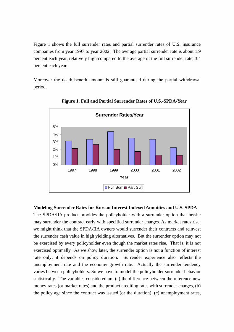
Figure 1 shows the full surrender rates and partial surrender rates of U.S. insurancecompanies from year 1997 to year 2002. The average partial surrender rate is about 1.9percent each year, relatively high compared to the average of the full surrender rate, 3.4percent each year.

Moreover the death benefit amount is still guaranteed during the partial withdrawalperiod.

Figure 1. Full and Partial Surrender Rates of U.S.-SPDA/Year

Surrender Rates/Year

0%

1%

2%

3%

4%

5%

1997 1998 1999 2000 2001 2002

Year

Full Surr Part Surr

Modeling Surrender Rates for Korean Interest Indexed Annuities and U.S. SPDAThe SPDA/IIA product provides the policyholder with a surrender option that he/shemay surrender the contract early with specified surrender charges. As market rates rise,we might think that the SPDA/IIA owners would surrender their contracts and reinvestthe surrender cash value in high yielding alternatives. But the surrender option may notbe exercised by every policyholder even though the market rates rise. That is, it is notexercised optimally. As we show later, the surrender option is not a function of interestrate only; it depends on policy duration. Surrender experience also reflects theunemployment rate and the economy growth rate. Actually the surrender tendencyvaries between policyholders. So we have to model the policyholder surrender behaviorstatistically. The variables considered are (a) the difference between the reference newmoney rates (or market rates) and the product crediting rates with surrender charges, (b)the policy age since the contract was issued (or the duration), (c) unemployment rates,

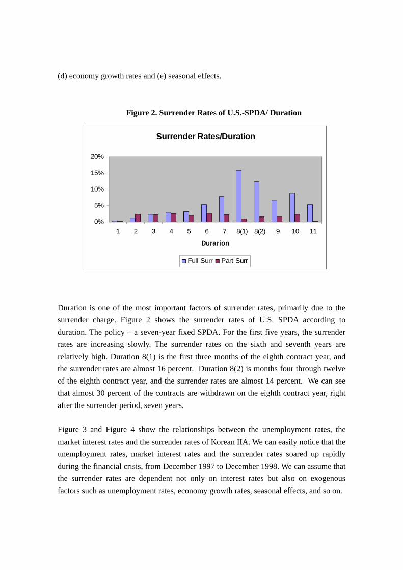
(d) economy growth rates and (e) seasonal effects.

Figure 2. Surrender Rates of U.S.-SPDA/ Duration

Surrender Rates/Duration

0%

5%

10%

15%

20%

1 2 3 4 5 6 7 8(1) 8(2) 9 10 11

Durarion

Full Surr Part Surr

Duration is one of the most important factors of surrender rates, primarily due to thesurrender charge. Figure 2 shows the surrender rates of U.S. SPDA according toduration. The policy – a seven-year fixed SPDA. For the first five years, the surrenderrates are increasing slowly. The surrender rates on the sixth and seventh years arerelatively high. Duration 8(1) is the first three months of the eighth contract year, andthe surrender rates are almost 16 percent. Duration 8(2) is months four through twelveof the eighth contract year, and the surrender rates are almost 14 percent. We can seethat almost 30 percent of the contracts are withdrawn on the eighth contract year, rightafter the surrender period, seven years.

Figure 3 and Figure 4 show the relationships between the unemployment rates, themarket interest rates and the surrender rates of Korean IIA. We can easily notice that theunemployment rates, market interest rates and the surrender rates soared up rapidlyduring the financial crisis, from December 1997 to December 1998. We can assume thatthe surrender rates are dependent not only on interest rates but also on exogenousfactors such as unemployment rates, economy growth rates, seasonal effects, and so on.

Figure 3. Unemployment Rates and Surrender Rates of Korean IIA

Unemployment and Surrender Rates

0%

2%

4%

6%

8%

10%

9701

9705

9709

9801

9805

9809

9901

9905

9909

0001

0005

0009

0101

0105

0109

0201

Unemployment Rates Surrender Rates

Source: Unemployment Rate; Korea National Statistical Office (www.nso.go.kr)

Figure 4. Market Interest Rates and Surrender Rates of Korean IIA

Surrender Rates/Market Rates of Korean IIA

0%

5%

10%

15%

20%

25%

30%

35%

9701

9704

9707

9710

9801

9804

9807

9810

9901

9904

9907

9910

0001

0004

0007

0010

0101

0104

0107

0110

0201

Market Rates Surrender Rates

Source: Market Rates; 5-year government bond rates; The Bank of Korea (www.ecos.bok.or.kr)

I prefer to use the logit link function in modeling the surrender rates of Korean IIA andU.S. SPDA. The logit functions is often used for modeling odds and probability

functions. There are many examples in which logit functions are used for financial dataanalysis. Hall (2000) compares logit analysis of data to the results from his prepaymentmodel. Pinder (1996) demonstrates how multinomial Logit Models can be used in adecision analysis framework to estimate expected monetary value. Kolari, Glennon,Shin and Caputo (2002) use the parametric approach of logit analysis to predict largecommercial bank failures. See also Johnsen and Melicher (1994), and Lo (1986).

To fit our data to the Logit Model, I used the Generalized Linear Models2, ProcedureGENMOD, Logistic Regression Models and Procedure LOGISTIC, with SAS3.

The Logit function has the following form,

⎟⎟⎠

⎞⎜⎜⎝

⎛− s

s

qq

1ln = 0β + 1β 1V + … + nβ nV , (1)

where sq is the surrender rate, iβ is the coefficient to be estimated and iV is theexplanatory variable.

For Korean IIA surrender rate models with 3 year duration4, we use the Logit Model,

⎟⎟⎠

⎞⎜⎜⎝

⎛− )(1

)(ln

tqtq

s

s = 0β + ∑

= 12,10,8,6,4,2,0jjβ

*( mi (t–j) – ci (t–j))

+ UEβ * UEi (t) + EGβ * EGi (t) + ∑=

−

11

1jjmonthβ *DVj, (2)

where DVj is the seasonal effect dummy-variable.

The parameter estimates are shown in Table 1. It is interesting to note that theparameter UEβ for the unemployment rates is very large, 50.6348. It means that the

2 I refer the reader to a few books on generalized linear model such as Agresti (1996 and 2002), Harrell(2001), Kutner, Nachtschiem, and Wasserman (1996), McCullagh and Nelder (1989), Firth (1991), andMcCulloch and Searle (2000). 3 In programming with SAS, refer Allison (1999), and SAS Institute Inc. (1999).4 We can model surrender rates with the duration (policy age since issue date) as an explanatory variable.For more details see Appendix and Kim(2004a). We notice that almost 30 percent of the contracts arewithdrawn on the eighth contract year, right after the accumulation period, seven years, as shown inFigure 2. So duration is one of the main factors of the surrender rates. In this paper, we want toinvestigate the policyholder surrender behaviors under extreme financial conditions. So we just look atthe contracts with the same duration; three years for Korean IIA and five years for U.S. SPDA, this willhelp us to check the impacts on the surrender rates due to the economic variables.

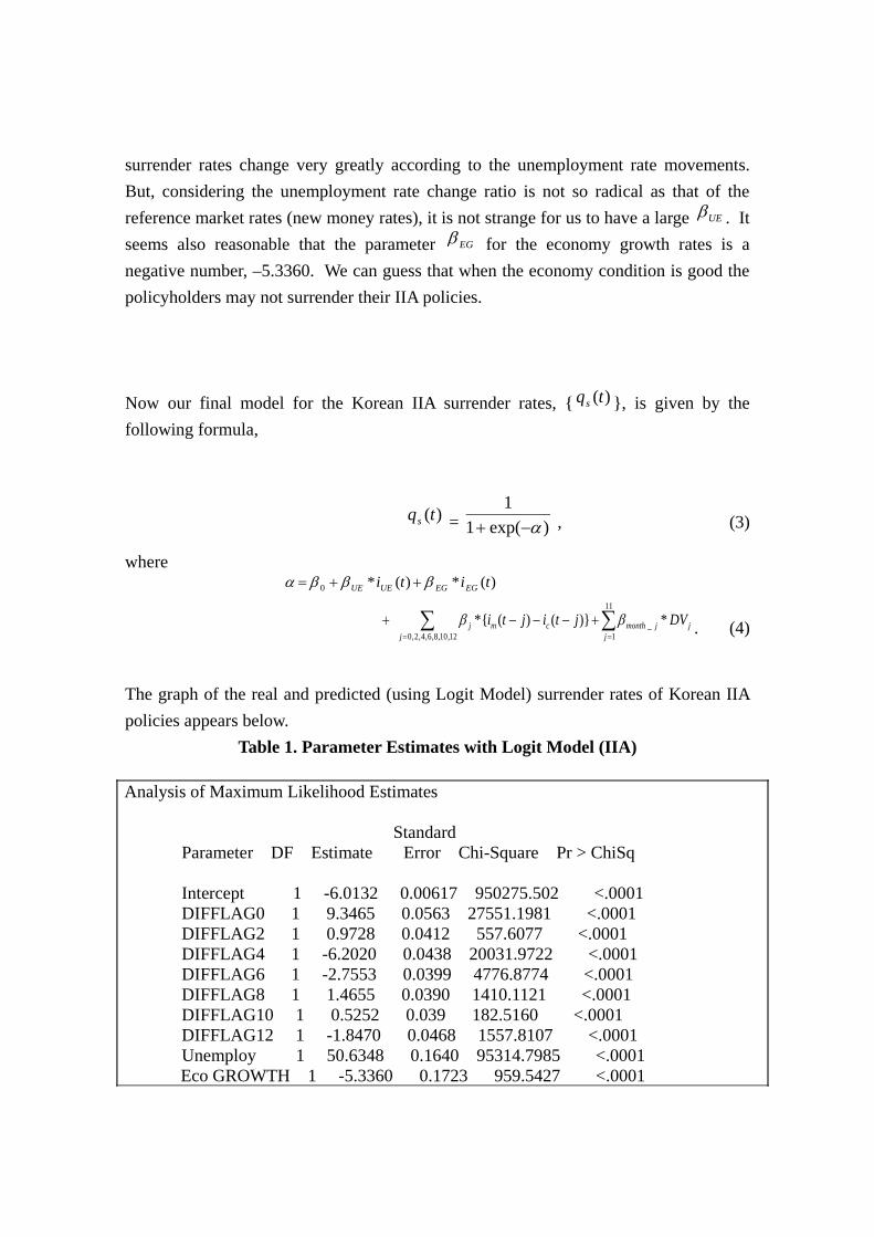
surrender rates change very greatly according to the unemployment rate movements.But, considering the unemployment rate change ratio is not so radical as that of thereference market rates (new money rates), it is not strange for us to have a large UEβ . Itseems also reasonable that the parameter EGβ for the economy growth rates is anegative number, –5.3360. We can guess that when the economy condition is good thepolicyholders may not surrender their IIA policies.

Now our final model for the Korean IIA surrender rates, { )(tqs }, is given by thefollowing formula,

)(tqs = )exp(11

α−+ , (3)

where )(*)(*0 titi EGEGUEUE βββα ++=

∑ ∑= =

+−−−+12,10,8,6,4,2,0

11

1_ *)}()({*

j jjjmonthcmj DVjtijti ββ . (4)

The graph of the real and predicted (using Logit Model) surrender rates of Korean IIApolicies appears below.

Table 1. Parameter Estimates with Logit Model (IIA)

Analysis of Maximum Likelihood Estimates

Standard Parameter DF Estimate Error Chi-Square Pr > ChiSq

Intercept 1 -6.0132 0.00617 950275.502 <.0001 DIFFLAG0 1 9.3465 0.0563 27551.1981 <.0001 DIFFLAG2 1 0.9728 0.0412 557.6077 <.0001 DIFFLAG4 1 -6.2020 0.0438 20031.9722 <.0001 DIFFLAG6 1 -2.7553 0.0399 4776.8774 <.0001 DIFFLAG8 1 1.4655 0.0390 1410.1121 <.0001 DIFFLAG10 1 0.5252 0.039 182.5160 <.0001 DIFFLAG12 1 -1.8470 0.0468 1557.8107 <.0001 Unemploy 1 50.6348 0.1640 95314.7985 <.0001

Eco GROWTH 1 -5.3360 0.1723 959.5427 <.0001

MONTH1 1 -0.2111 0.00409 2662.3227 <.0001 MONTH2 1 -0.4199 0.00446 8867.3221 <.0001 MONTH3 1 -0.3629 0.00446 6633.6120 <.0001 MONTH4 1 0.1121 0.00415 728.9672 <.0001 MONTH5 1 0.2443 0.00408 3589.7187 <.0001 MONTH6 1 0.2961 0.00424 4879.2107 <.0001 MONTH7 1 0.2111 0.00429 2421.8388 <.0001 MONTH8 1 0.2082 0.00458 2065.2003 <.0001 MONTH9 1 0.4040 0.00452 7970.0766 <.0001 MONTH10 1 0.4919 0.00469 11024.0567 <.0001 MONTH11 1 0.3720 0.00447 6913.5047 <.0001

Figure 5. Real and Predicted Surrender Rates of Korean IIA

9801

9804

9807

9810

9901

9904

9907

9910

0001

0004

0007

0010

0101

0104

0107

0110

0201

For U.S. SPDA surrender rate models with fiveyear duration, we also use the LogitModel,

⎟⎟⎠

⎞⎜⎜⎝

⎛− )(1

)(ln

tqtq

s

s = 0β + Mβ *( mi (t) – ci (t)) + UEβ * UEi (t) + EGβ * EGi (t) , (5)

where Mβ is the parameter for the difference between current reference market ratesand policy crediting rates.

The parameter estimates are shown in Table 2. We can notice that the parameter UEβ

for the unemployment rates is 24.3694 very smaller than that of the Korean IIAunemployment parameter, 50.6348. It means that the U.S. SPDA surrender rates changeless sensitively according to the unemployment rate movements. It seems alsoreasonable that the parameter EGβ for the economy growth rates is a negative number, –2.6450.

For the U.S. SPDA, the surrender rates, { )(tqs }, are estimated using the followingformula,

)(tqs = )exp(11

α−+ , (6)

where: α = 0β + Mβ *( mi (t) – ci (t)) + UEβ * UEi (t) + EGβ * EGi (t). (7)

The graph of the real and predicted (using Logit Model) surrender rates of U.S. SPDApolicies is shown below. The average of the real surrender rates is 2.97 percent and theaverage of the expected (predicted) surrender rates using Logit Model is 2.92 percent.

Table 2. Parameter Estimates with Logit Model (U.S. SPDA)

Analysis of Maximum Likelihood Estimates


Intercept 1 -4.5452 0.00785 89325.4212 <.0001 DIFFLAG 1 12.7525 0.05831 25413.1981 <.0001 Unemploy 1 24.3694 0.27836 59821.6548 <.0001

Eco GROWTH 1 -2.6450 0.86473 4862.2485 <.0001

Figure 6. Real and Predicted Surrender Rates of U.S. SPDA

Surrender Rate Changes Under Financial Rate ShocksThere are many factors affecting surrender rates such as the difference betweenreference market rate and policy crediting rate, seasonal effect, age and gender ofclients, economy growth rate, foreign exchange rate, inflation rate, policy age sinceissue date (duration) and unemployment rate, among others. During the stable interestrate period, all of these factors play an important role in determining the surrender rate.But sometimes, if there are any shocks (or sudden changes) on financial rates, such asthe unemployment rates, the economy growth rates, or the market interest rates, thesurrender rates can be changed much more than expected. For example, during thefinancial crisis in Korea from December 1997 to December 1998, the surrender ratesshow a sudden peak. Figure 4 shows the sudden increase in the market interest rates during the financialcrisis and the surrender rates of Korean IIA, and we can see that interest rate fluctuationis really an important factor in determining the surrender rates. Figure 3 shows theunemployment rates and the surrender rates of Korean IIA. We can easily see that theunemployment rates and surrender rates soared up during the financial crisis.Therefore, we can assume that the surrender rates are dependent not only on interestrates but also on exogenous factors such as unemployment rates, economy growth rates,seasonal effects, and so on.

0.00%

0.50%

1.00%

1.50%

2.00%

2.50%

3.00%

3.50%

4.00%

4.50%

9701

9704

9707

9710

9801

9804

980798

1099

0199

0499

0799

1000

01000

400

070010

0101

010401

0701

1002

0102

0402

0702

10

Time

Expected Real

Now we want to investigate the surrender rate changes under the assumption that thereare financial rate shocks (or sudden changes). As an example, we first look at thepattern of the financial rate shocks during the Korean financial crisis.

Let us denote )(ti to be a financial rate at time t. We use the following formula for thefinancial rate at time t,

)(ti = μ + k(t) σ , (8)where μ is the average and σ is the standard deviation of the financial rate during astable state period.

We define k(t) to be a risk measure of the financial rate )(ti ,

k(t) = σμ−)(ti

. (9)

We define that the financial rate )(ti experiences a financial rate shock at time t if|k(t)| ≥ 2, (10)

and we say that the financial rate is in a stable status at time t if |k(t)| < 2. We also saythat we are under extreme financial conditions if the financial rates experience financialrate shocks.

Figure 7 shows the risk measure k(t) of the reference market rates (five-yeargovernment bond rates), the unemployment rates and the economy growth rates ofKorea around the financial crisis period.

Figure 7. Risk Measure, k(t), of Korean Financial Rates

Risk measure, k(t)

-10

-5

0

5

10

15

20

9706 9709 9712 9803 9806 9809 9812 9903 9906 9909 9912

k(t)

Market rates Unemployment Economy growth

Source: Market Rates; 5-year government bond rates; The Bank of Korea (www.ecos.bok.or.kr)

Unemployment Rate ; Korea National Statistical Office (www.nso.go.kr)

Economy Growth Rates ; Korean Statistical Information System (www.kosis.nso.go.kr)

From Figure 7, we can see that the market rates experience financial shocks, k(t) > 2,for the period from July of 1997 to September of 1998, for 14 months around thefinancial crisis. The unemployment rates experience financial shocks, k(t) ≥ 2, for theperiod from February of 1998 to August of 1999, for 19 months around the financialcrisis. The economy growth rates experience financial shocks, k(t) ≤ -2, for the periodfrom November of 1997 to March of 1998, for five months around the financial crisis.

Figure 5 shows the real and expected surrender rates (using Logit Model) of Korean IIAconsidering all of the financial rate shocks. The averages of the real and expected(predicted) surrender rates of Korean IIA are 4.2 percent. Now, we want to consider the surrender rate changes of U.S. SPDA under theassumption that U.S. financial rates experience the financial rate shocks. We made twoassumptions on the pattern of k(t), the risk measures of the financial rates. Assumption1 (A1): the pattern of k(t) is same as that of Korean data when the rate experiencesfinancial shocks. When the rate does not experience any financial shocks, the riskmeasure k(t) is calculated from U.S. data. Assumption 2 (A2): k(t) = c, where c is aconstant integer such that |c| ≥ 2 and the financial rate )(ti is changed to σcti +)( .

Figure 8 shows the surrender rate changes of U.S. SPDA under the assumption (A1) thatthe U.S. market rates (10 year T-bond rates) experience the financial rate shock, k(t) ≥

2, as the same pattern of k(t) as that of Korean data.

It shows a very high peak of 12.63 percent at the beginning of the market rate shockperiod. The average of the expected (predicted) surrender rates is 3.42 percent whereasthe average of the real surrender rates is 2.97 percent.

Figure 8. U.S. SPDA Surrender Rate Changes under Market Rate Shock(A1)

Surrender rates under market rate shock(A1)

0%

2%

4%

6%

8%

10%

12%

14%

Expected Surr Rates Real Surr Rates

Figure 9. U.S. SPDA Surrender Rate Changes under Market Rate Shock (A2)

Surrender rates under Market rate shock (A2)

0%

1%

2%

3%

4%

5%

6%

7%

Real Surr Rates k(t) = 2 k(t) = 3 k(t) = 5

Figure 9 shows the surrender rate changes of U.S. SPDA under the assumption (A2) thatthe U.S. market rates (10-year T-bond rates) experience the financial rate shock, k(t) =2, 3, 5 over the whole period.

It shows that the surrender rates are increasing as k(t) goes up, i.e., market ratesincrease. The average of the expected (predicted) surrender rates is 3.49 percent whenk(t) = 2, 3.82 percent when k(t) = 3, and 4.56 percent when k(t) = 5, whereas theaverage of the real surrender rates is 2.97 percent.

Figure 10 shows the surrender rate changes of U.S. SPDA under the assumption (A1)that the U.S. unemployment rates experience the financial rate shock, k(t) ≥ 2, as thesame pattern of k(t) as that of Korean data.

It shows a very high peak of 7.56 percent in the middle of the unemployment rate shockperiod. We also notice the interesting point that the unemployment rate shock periodstarts later than that of market rate shock, and lasts longer. The average of the expected(predicted) surrender rates is 3.42 percent, whereas the average of the real surrenderrates is 2.97 percent.

Figure 10. U.S. SPDA Surrender Rate Changes Under Unemployment Rate Shock(A1)

Surrender rates under unemployment rate shock (A1)

0%

1%

2%

3%

4%

5%

6%

7%

8%


Figure 11 shows the surrender rate changes of U.S. SPDA under the assumption (A2)that the U.S. unemployment rates experience the financial rate shock, k(t) = 2, 3, 5 overthe whole period.

It shows that the surrender rates are increasing as k(t) goes up, i.e., unemployment ratesincrease. The average of the expected (predicted) surrender rates is 3.94 percent whenk(t) = 2, 4.57 percent when k(t) = 3, and 6.13 percent when k(t) = 5, whereas theaverage of the real surrender rates is 2.97 percent.

Figure 11. U.S. SPDA Surrender Rate Changes under Unemployment Rate Shock(A2)

Surrender rates under Unemployment rate shock (A2)

0%

1%2%

3%4%

5%6%

7%8%

9%

Real Surr Rates k(t) = 2 k(t) = 3 k(t) = 5

Figure 12 shows the surrender rate changes of U.S. SPDA under the assumption (A1)that the U.S. economy growth (GDP) rates experience the financial rate shock, k(t) ≤ -2, as the same pattern of k(t) as that of Korean data.

It shows a small peak of 3.89 percent in the beginning of the shock period. We can seethat the economy growth rate shock period lasts for short periods of five months and theimpacts of the economy growth rate shock to surrender rates are relatively small. Theaverage of the expected (predicted) surrender rates is 2.98 percent, whereas the averageof the real surrender rates is 2.97 percent.

Figure 12. U.S. SPDA Surrender Rate Changes Under Economy Growth RateShock (A1)

Surrender rates under Economy growth rate shock (A1)

0%

1%

1%

2%

2%

3%

3%

4%

4%

5%


Figure 13 shows the surrender rate changes of U.S. SPDA under the assumption (A2)that the U.S. economy growth (GDP) rates experience the financial rate shock, k(t) = -2,-3, -5 over the whole period.

It shows that the surrender rates are increasing as k(t) goes down, i.e., the economygrowth rates decrease. The average of the expected (predicted) surrender rates is 3.27percent when k(t) = -2, 3.46 percent when k(t) = -3, and 3.87 percent when k(t) = -5,whereas the average of the real surrender rates is 2.97 percent.

Figure 13. U.S. SPDA Surrender Rate Changes Under Economy Growth RateShock (A2)

Surrender rates under Economy growth rate shock (A2)

0%

1%

2%

3%

4%

5%

6%

Real Surr Rates k(t) = -2 k(t) = -3 k(t) = -5

Figure 14. U.S. SPDA Surrender Rate Changes Under Total Rate Shock (A1)

Surrender rates under Total rate shock (A1)

0%

2%

4%

6%

8%

10%

12%

14%

16%


Figure 14 shows the surrender rate changes of U.S. SPDA under the assumption (A1)that the total three U.S. financial rates (market, unemployment and economy growthrates) experience the financial rate shock, |k(t)| ≥ 2, at the same time, as the samepattern of k(t) as that of Korean data.

It shows a high peak of 14.71 percent at the beginning of the shock period. And thesurrender rates are quite high with the average of 7.67 percent during the shock periodfor almost two years. The average of the expected (predicted) surrender rates is 4.48percent, whereas the average of the real surrender rates is 2.97 percent.

ConclusionMany insurance companies are selling single premium deferred annuities (SPDA). ButSPDA are sold with the primary focus on accumulation. Only a few of the policyholderspurchase SPDA for the purpose of annuitization. In Korea, the annuity market is stillyoung and growing slowly compared to that of the United States (U.S.). Interest-indexed annuities (IIA) are one of the most popular SPDA products in Korea. Thedistinctive features of SPDA are the surrender options and annuitization options. In thispaper we consider the surrender behaviors of SPDA /IIA policyholders under extremeeconomic conditions.

We have considered a model on the policyholder surrender behavior statistically. Thevariables considered are the difference between reference market rates and productcrediting rates with surrender charges, the policy age since the contract was issued,unemployment rates, economy growth rates and seasonal effects. Especially theduration, i.e., the policy age since the contract was issued, is one of the most importantfactors of surrender rates. We use the Logit Model for the surrender rates.

For extreme events/financial rate shocks, we define k(t), a risk measure of a financialrate )(ti ,

k(t) = σμ−)(ti

.

We define that the financial rate )(ti experiences a financial rate shock at time t if|k(t)| ≥ 2,

and we say that the financial rate is in a stable status at time t if |k(t)| < 2. We also saythat we are under extreme financial conditions if the financial rates experience financialrate shocks.

We considered the surrender rate changes of U.S. SPDA under the assumption that U.S.financial rates experience the financial rate shocks. We make two assumptions on thepattern of k(t), the risk measures of the financial rates. Assumption 1 (A1): the patternof k(t) is the same as that of Korean data when the rate experiences financial shocks.When the rate does not experience any financial shocks, the risk measure k(t) iscalculated from U.S. data. Assumption 2 (A2): k(t) = c, where c is a constant integersuch that |c| ≥ 2 and the financial rate )(ti is changed to σcti +)( . We summarized theanalysis results in the following table.

Table 3. Surrender Rate Changes under Extreme ConditionsMarket rates Unemployment rates Economy Growth rates Total rates

Assumption max average max average max average max averageA1 12.63% 3.42% 7.56% 3.66% 3.89% 2.96% 14.71% 4.48%

|k(t)| = 2 4.62% 3.49% 5.20% 3.94% 4.32% 3.27% 9.23% 4.37%|k(t)| = 3 5.04% 3.82% 6.02% 4.57% 4.57% 3.46% 11.57% 6.24%|k(t)| = 5 6.01% 4.56% 8.04% 6.13% 5.11% 3.87% 15.03% 10.85%

From Table 3, we can see that the surrender rates change very much under extremeconditions. We see a high peak of 14.71 percent when all of the three variablesexperience financial rate shocks under the assumption 1. And the surrender rates arequite high with the average of 7.67 percent during the shock period for almost twoyears. The average of the expected (predicted) surrender rates is 4.48 percent, whereasthe average of the real surrender rates (without extreme condition assumptions) is 2.97percent. It may be a consideration in risk management of insurance business to predict suddenincrease of surrender rates and prepare appropriate hedging strategies.

Appendix Modeling Surrender Rates of Korean Annuities We wanted to show a method to model surrender rates with economic variables anddurations (policy age since issue date) for Korean annuities. Therefore, we e showedhow to choose the explanatory variables. We also showed how to compare the surrenderrate models and choose a better model for Korean annuities. This method can be appliedto other insurance policies.

Variables and AssumptionsFollowing is a summary of the explanatory variables and the assumptions used inmodeling the surrender rates of Korean annuities.

Table A1. Explanatory Variables Considered

Variable Contents MemoBASEYM Year, Month of dataDIFFLAG0 Difference of rates =market rate-crediting rate at current timeDIFFLAG2 Difference of rates =market rate-crediting rate 2 months agoDIFFLAG4 〃 =market rate-crediting rate 4 months agoDIFFLAG6 〃 =market rate-crediting rate 6 months agoDIFFLAG8 〃 =market rate-crediting rate 8 months agoDIFFLAG10 〃 =market rate-crediting rate 10 months agoDIFFLAG12 〃 =market rate-crediting rate 12 months agoPOL-AGE Policy age Average policy age since issueLOST Unemployment ratesGROWTH Economy growth ratesIMF Financial crisis period

under IMF controlPeriod from 1997.12 to 1998.12

Dummy variable = 1 during the periodMONTH1 January Dummy variable = 1 on current monthMONTH2 February 〃MONTH3 March 〃MONTH4 April 〃MONTH5 May 〃MONTH6 Jun 〃MONTH7 July 〃MONTH8 August 〃MONTH9 September 〃MONTH10 October 〃MONTH11 November 〃SUR_RATE Real surrender rate Dependent variables

For seasonal effects, we investigated the surrender rates from January to November. Weconsidered the financial crisis period since the surrender rates skyrocketed during thisperiod. We used dummy variable 1 during the financial crisis period from Dec. 1997 toDec. 1998 and 0 elsewhere.

The dependent variable SUR_RATE denotes the real surrender rates, and it is the faceamount of surrendered policies divided by the face amount of initial policies. Weconsider Korean annuities with more than 1,000,000 policyholders.5

Surrender Rate Models

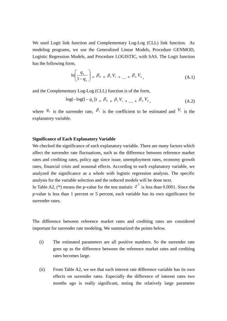
We used Logit link function and Complementary Log-Log (CLL) link function. Asmodeling programs, we use the Generalized Linear Models, Procedure GENMOD,Logistic Regression Models, and Procedure LOGISTIC, with SAS. The Logit functionhas the following form,

⎟⎟⎠

⎞⎜⎜⎝

⎛− s

s

qq

1ln = 0β + 1β 1V + … + nβ nV , (A.1)

and the Complementary Log-Log (CLL) function is of the form,

))1log(log( sq−− = 0β + 1β 1V + … + nβ nV , (A.2)

where sq is the surrender rate, iβ is the coefficient to be estimated and iV is theexplanatory variable.

Significance of Each Explanatory Variable We checked the significance of each explanatory variable. There are many factors whichaffect the surrender rate fluctuations, such as the difference between reference marketrates and crediting rates, policy age since issue, unemployment rates, economy growthrates, financial crisis and seasonal effects. According to each explanatory variable, weanalyzed the significance as a whole with logistic regression analysis. The specificanalysis for the variable selection and the reduced models will be done next.In Table A2, (*) means the p-value for the test statistic

2χ is less than 0.0001. Since thep-value is less than 1 percent or 5 percent, each variable has its own significance forsurrender rates.

The difference between reference market rates and crediting rates are consideredimportant for surrender rate modeling. We summarized the points below.

(i) The estimated parameters are all positive numbers. So the surrender rategoes up as the difference between the reference market rates and creditingrates becomes large.

(ii) From Table A2, we see that each interest rate difference variable has its owneffects on surrender rates. Especially the difference of interest rates twomonths ago is really significant, noting the relatively large parameter

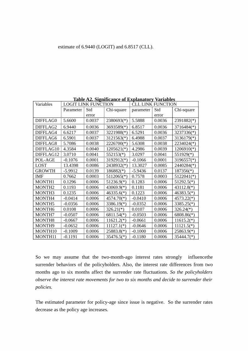
estimate of 6.9440 (LOGIT) and 6.8517 (CLL).

Table A2. Significance of Explanatory VariablesVariables LOGIT LINK FUNCTION CLL LINK FUNCTION

Parameter Stderror

Chi-square parameter Stderror

Chi-square

DIFFLAG0 5.6600 0.0037 2380693(*) 5.5888 0.0036 2391882(*)DIFFLAG2 6.9440 0.0036 3693589(*) 6.8517 0.0036 3716484(*)DIFFLAG4 6.6217 0.0037 3221988(*) 6.5291 0.0036 3237336(*)DIFFLAG6 6.5901 0.0037 3121563(*) 6.4988 0.0037 3136179(*)DIFFLAG8 5.7086 0.0038 2226700(*) 5.6308 0.0038 2234024(*)DIFFLAG10 4.3584 0.0040 1205621(*) 4.2986 0.0039 1206910(*)DIFFLAG12 3.0710 0.0041 552153(*) 3.0297 0.0041 551929(*)POL-AGE -0.1076 0.0001 3192912(*) -0.1066 0.0001 3196557(*)LOST 13.4398 0.0086 2438932(*) 13.3027 0.0085 2440284(*)GROWTH -5.9912 0.0139 186882(*) -5.9436 0.0137 187356(*)IMF 0.7662 0.0003 5112065(*) 0.7578 0.0003 5122041(*)MONTH1 0.1296 0.0006 51236.9(*) 0.1283 0.0006 51292.5(*)MONTH2 0.1193 0.0006 43069.9(*) 0.1181 0.0006 43112.8(*)MONTH3 0.1235 0.0006 46335.6(*) 0.1223 0.0006 46383.5(*)MONTH4 -0.0414 0.0006 4574.70(*) -0.0410 0.0006 4573.22(*)MONTH5 -0.0356 0.0006 3386.19(*) -0.0352 0.0006 3385.25(*)MONTH6 0.0108 0.0006 326.21(*) 0.0107 0.0006 326.24(*)MONTH7 -0.0507 0.0006 6811.54(*) -0.0503 0.0006 6808.86(*)MONTH8 -0.0667 0.0006 11621.2(*) -0.0661 0.0006 11615.2(*)MONTH9 -0.0652 0.0006 11127.1(*) -0.0646 0.0006 11121.5(*)MONTH10 -0.1009 0.0006 25883.8(*) -0.1000 0.0006 25863.9(*)MONTH11 -0.1191 0.0006 35476.5(*) -0.1180 0.0006 35444.7(*)

So we may assume that the two-month-ago interest rates strongly influencethesurrender behaviors of the policyholders. Also, the interest rate differences from twomonths ago to six months affect the surrender rate fluctuations. So the policyholdersobserve the interest rate movements for two to six months and decide to surrender theirpolicies.

The estimated parameter for policy-age since issue is negative. So the surrender ratesdecrease as the policy age increases.

The positive parameter for unemployment rates indicates that surrender rates go upwhen the unemployment rates increase. It is natural and it is really significant to takethe unemployment rates into account as an explanatory variable in modeling surrenderrates considering the relatively high parameter estimate of 13.4398 (LOGIT) and13.3027 (CLL).

The parameter for economy growth rates is negative and we may think that thesurrender rates go down under good economy conditions.

The positive parameter for the dummy variable, financial crisis under IMF control,means that the surrender rates can increase when unexpected economy/finance shockhappens.

It is interesting to note that the parameters for January, February, March, and June arepositive and the others are negative, but all are small. Thus the season has a small effecton surrender behavior.

Reduced Models We may not need all of the variables in modeling surrender rates, i.e., the fullinformation model. In this section, we found appropriate reduced models with leastnumber of explanatory variables for Korean annuities. We worked to keep the same fitwith the reduced model as that of the full information model. We know that there are afew methods, such as forward selection method, backward elimination method, stepwiseregression, and all possible regressions, to select the most significant variables. We followed three steps to find the most appropriate reduced models. The first step wasto select a few significant explanatory variables with the backward elimination method.The second step was to set up reduced models with the selected variables. The third stepwas to transform the policy age (or duration). The reason we transformed the policy ageis that there is a possibility that the fit may become worse if we use the real policy agewithout transformation.

Also, we compared the three models, Arctangent Model, Logit Model and CLL model,and chose the most appropriate one for Korean annuities.6

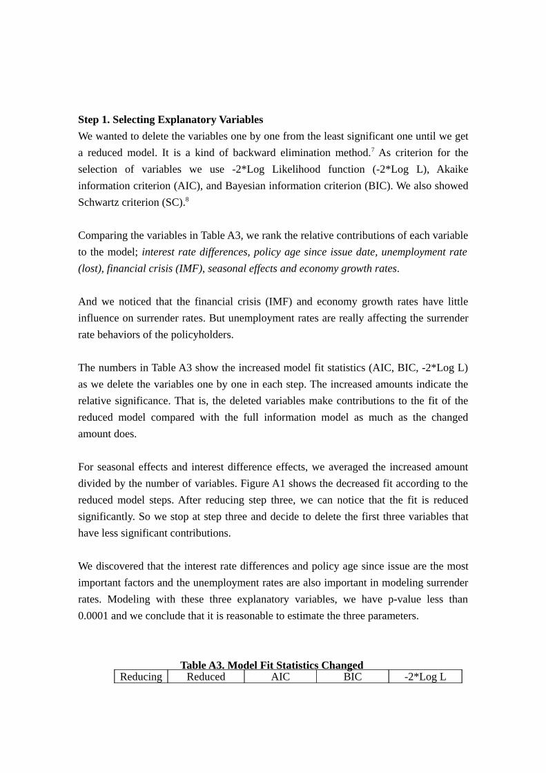
Step 1. Selecting Explanatory Variables We wanted to delete the variables one by one from the least significant one until we geta reduced model. It is a kind of backward elimination method.7 As criterion for theselection of variables we use -2*Log Likelihood function (-2*Log L), Akaikeinformation criterion (AIC), and Bayesian information criterion (BIC). We also showedSchwartz criterion (SC).8

Comparing the variables in Table A3, we rank the relative contributions of each variableto the model; interest rate differences, policy age since issue date, unemployment rate(lost), financial crisis (IMF), seasonal effects and economy growth rates.

And we noticed that the financial crisis (IMF) and economy growth rates have littleinfluence on surrender rates. But unemployment rates are really affecting the surrenderrate behaviors of the policyholders.

The numbers in Table A3 show the increased model fit statistics (AIC, BIC, -2*Log L)as we delete the variables one by one in each step. The increased amounts indicate therelative significance. That is, the deleted variables make contributions to the fit of thereduced model compared with the full information model as much as the changedamount does.

For seasonal effects and interest difference effects, we averaged the increased amountdivided by the number of variables. Figure A1 shows the decreased fit according to thereduced model steps. After reducing step three, we can notice that the fit is reducedsignificantly. So we stop at step three and decide to delete the first three variables thathave less significant contributions.

We discovered that the interest rate differences and policy age since issue are the mostimportant factors and the unemployment rates are also important in modeling surrenderrates. Modeling with these three explanatory variables, we have p-value less than0.0001 and we conclude that it is reasonable to estimate the three parameters.

Table A3. Model Fit Statistics Changed Reducing Reduced AIC BIC -2*Log L

step variable1 Economy growth 45 27 47 2 Seasonal 2,039 2,021 2,041 3 IMF 9,015 8,998 9,017 4 Unemployment 29,162 29,144 29,164 5 Policy age 1,127,643 1,127,625 1,127,645 6 Interest diff. 251,787 251,769 251,789

Figure A1. Model Fit Statistics Changed

0

200,000

400,000

600,000

800,000

1,000,000

1,200,000

1 2 3 4 5 6

AIC

BIC

-2*Log L

For Korean annuity, we selected policy age, interest rate differences and unemploymentrates as the explanatory variables.

Step 2. Reduced Models The second step included set up of reduced models with the selected variables from step1. We present three tables. The first and second tables show the estimated parameters forthe selected variables from Logit and CLL model. The third table shows the estimatederrors for the three models, Arctangent Model, Logit Model and CLL Model, and alsocompares the models by the differences of the estimated errors between ArctangentModel, Logit Model, Arctangent Model and CLL Model according to the policy agesince issue9. For comparison purposes, we define RMSE and MAPE as follows,

RMSE = nyy ii∑ − 2)ˆ(

, (A.3)

and

MAPE = n1 ∑

−

i

ii

yyy ˆ

, (A.4)

where, iy is the i-th real value, iy is the i-th predicted value, and n is the sample size.

We defined the terminologies used in the third table as follows. RMSE1 is RMSE ofArctangent Model, RMSE2 is RMSE of Logit Model, and RMSE3 is RMSE of CLLModel. MAPE1, MAPE2 and MAPE3 represent the MAPE of Arctangent Model, LogitModel and CLL Model respectively.RMSEGAP1 denotes RMSE1-RMSE2, so Logit Model is better than Arctangent Modelif RMSEGAP1 is positive. RMSEGAP2 is RMSE1-RMSE3, so CLL Model is betterthan Arctangent Model if RMSEGAP2 is positive. MAPEGAP1 is MAPE1-MAPE2 andLogit Model is better than Arctangent Model if MAPEGAP1 is positive. MAPEGAP2 isMAPE1-MAPE3 and CLL Model is better than Arctangent Model if MAPEGAP2 ispositive.

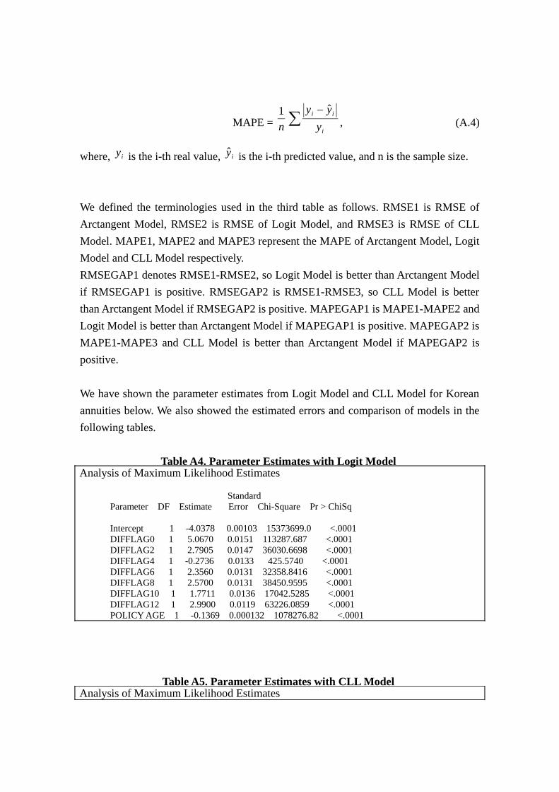
We have shown the parameter estimates from Logit Model and CLL Model for Koreanannuities below. We also showed the estimated errors and comparison of models in thefollowing tables.

Table A4. Parameter Estimates with Logit Model Analysis of Maximum Likelihood Estimates


Intercept 1 -4.0378 0.00103 15373699.0 <.0001 DIFFLAG0 1 5.0670 0.0151 113287.687 <.0001 DIFFLAG2 1 2.7905 0.0147 36030.6698 <.0001 DIFFLAG4 1 -0.2736 0.0133 425.5740 <.0001 DIFFLAG6 1 2.3560 0.0131 32358.8416 <.0001 DIFFLAG8 1 2.5700 0.0131 38450.9595 <.0001 DIFFLAG10 1 1.7711 0.0136 17042.5285 <.0001 DIFFLAG12 1 2.9900 0.0119 63226.0859 <.0001 POLICY AGE 1 -0.1369 0.000132 1078276.82 <.0001

Table A5. Parameter Estimates with CLL Model Analysis of Maximum Likelihood Estimates



Table A6. Estimated Errors and Comparison of Models time RMSE1 RMSE2 RMSE3 MAPE1 MAPE2 MAPE3 RMSEGAP1 RMSEGAP2 MAPEGAP1 MAPEGAP2

0.5 0.02707 0.02083 0.02078 0.3268 0.29949 0.29887 0.00624 0.00629 0.02731 0.02792

1.5 0.00773 0.00858 0.00861 0.19563 0.22432 0.22502 -0.00084 -0.00088 -0.02869 -0.02939

2.5 0.00569 0.01358 0.01357 0.24269 0.95731 0.95601 -0.00789 -0.00788 -0.71462 -0.71332

3.5 0.00607 0.00903 0.00901 0.30749 0.76591 0.76488 -0.00296 -0.00294 -0.45841 -0.45739

4.5 0.007 0.00477 0.00475 0.24598 0.32145 0.32079 0.00223 0.00225 -0.07547 -0.07481

5.5 0.00734 0.00297 0.00301 0.20046 0.09406 0.09451 0.00437 0.00433 0.1064 0.10595

6.5 0.00869 0.00299 0.00304 0.7049 0.1216 0.1229 0.00569 0.00565 0.5833 0.582

7.5 0.00849 0.00386 0.0039 0.34024 0.20862 0.21083 0.00463 0.00459 0.13162 0.12941

8.5 0.00842 0.0039 0.00393 0.31219 0.20492 0.20738 0.00452 0.00449 0.10727 0.10481

9.5 0.00817 0.00452 0.00454 0.30694 0.20528 0.20597 0.00365 0.00363 0.10166 0.10097

For an annuity plan, we may not be able to conclude that Logit or CLL Model is betterthan Arctangent Model. Even when we added unemployment rates and IMF effects tothe Logit and CLL Models, we did not have enough evidence that one model was betterthan the other ones. Also the sign of DIFFLAG4 is negative and it seems to beunexplainable.

Step 3. Transformation of Duration The third step is to transform the policy age (duration) since issue. The reason wetransformed the policy age is that the surrender rates are dependent on durations andthere is the possibility that the fit may be decreased if we use the real policy age withouttransformation. We tried three formulas that are usually used in transformation10,

n x , xlog , and x1

− . (A.5)

The policy age may be transformed to

( )nagepolicy1

, log(policy age), or agepolicy1

− (A.6)

We chose the best transformation formula using the model fit statistics –2Log L.We compared Arctangent Model and Logit Model and Arctangent Model and CLLModel, and concluded which model is the best one.

Table A7. Model Fit Statistics According to Transformed Policy Age

Figure A2. Model Fit Statistics According to Transformed Policy Age

71500000

71600000

71700000

71800000

71900000

72000000

72100000

72200000

72300000

1 2 3 4 5 6 7 8 9 10

( )nagepolicy1 -2*Log L

n=1 72208277 n=2 71946654 n=3 71863316 n=4 71825035 n=5 71803493 n=6 71789797 n=7 71780359 n=8 71773477 n=9 71768243 n=10 71764133

Formula -2*Log LLog(policy age) 71730319 -1/(policy age) 71680566

Table A7 and Figure A2 show the model fit statistics (-2*Log L) according to the policyage. We noticed that the model fits well when we transform the policy age. Comparingthe model fit statistics, we concluded that the best transformation formula is

agepolicy1

− .

We have shown the analysis results in the following tables.

Table A8. Parameter Estimates with Logit Model under Transformation Analysis of Maximum Likelihood Estimates



LOST 1 10.5238 0.0617 29044.8354 <.0001

Table A9. Parameter Estimates with CLL Model under TransformationAnalysis of Maximum Likelihood Estimates


Intercept 1 -5.4089 0.00252 4597008.35 <.0001 DIFFLAG0 1 5.9574 0.0160 138442.495 <.0001 DIFFLAG2 1 1.8506 0.0153 14580.5856 <.0001 DIFFLAG4 1 -1.0303 0.0138 5583.9827 <.0001

DIFFLAG6 1 1.6172 0.0134 14475.6309 <.0001 DIFFLAG8 1 2.3250 0.0128 32949.0219 <.0001 DIFFLAG10 1 1.4808 0.0134 12166.9626 <.0001 DIFFLAG12 1 0.6886 0.0178 1491.4247 <.0001 POLICY AGE 1 -0.6561 0.000465 1991007.04 <.0001

LOST 1 10.4363 0.0610 29316.3498 <.0001

Table A10. Errors and Comparison of Models under Transformation time RMSE1 RMSE2 RMSE3 MAPE1 MAPE2 MAPE3 RMSEGAP1 RMSEGAP2 MAPEGAP1 MAPEGAP2

0.5 0.02707 0.01256 0.01274 0.3268 0.19366 0.19315 0.01451 0.01433 0.13314 0.13364

1.5 0.00773 0.00951 0.00954 0.19563 0.26445 0.26563 -0.00177 -0.00181 -0.06882 -0.06999

2.5 0.00569 0.00474 0.00474 0.24269 0.36096 0.36226 0.00095 0.00096 -0.11827 -0.11957

3.5 0.00607 0.00364 0.00368 0.30749 0.34218 0.34641 0.00243 0.00239 -0.03468 -0.03892

4.5 0.007 0.00258 0.00263 0.24598 0.13063 0.13339 0.00443 0.00437 0.11535 0.11259

5.5 0.00734 0.00463 0.00465 0.20046 0.16366 0.16235 0.00272 0.0027 0.0368 0.0381

6.5 0.00869 0.0029 0.00293 0.7049 0.11537 0.11695 0.00579 0.00576 0.58953 0.58795

7.5 0.00849 0.00281 0.00284 0.34024 0.24663 0.25122 0.00568 0.00565 0.09361 0.08902

8.5 0.00842 0.00305 0.00307 0.31219 0.30407 0.30834 0.00537 0.00535 0.00812 0.00385

9.5 0.00817 0.00351 0.00352 0.30694 0.29396 0.29819 0.00466 0.00465 0.01297 0.00875

When we did not transform the policy ages, we did not have enough evidence to suggestthat one model was better than the other ones. But Logit and CLL Models are betterthan the Arctangent Model on many policy ages after we transform the policy ages.

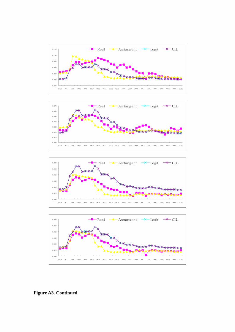
In conclusion, we show the 10 graphs of real and estimated surrender rates for each

model according to the policy age from duration one to duration 10 for Korean annuity.

Note that the Logit Model and the CLL Model produce almost the same results and the

two graphs are overlapping.

Figure A3. Surrender Rates According to the Policy Age (Duration)

0.000

0.020

0.040

0.060

0.080

0.100

0.120

9709 9711 9801 9803 9805 9807 9809 9811 9901 9903 9905 9907 9909 9911 0001 0003 0005 0007 0009 0011

Real Arctangent Logit CLL

0.000

0.010

0.020

0.030

0.040

0.050

0.060

0.070

9709 9711 9801 9803 9805 9807 9809 9811 9901 9903 9905 9907 9909 9911 0001 0003 0005 0007 0009 0011


0.000

0.010

0.020

0.030

0.040

0.050

0.060

9709 9711 9801 9803 9805 9807 9809 9811 9901 9903 9905 9907 9909 9911 0001 0003 0005 0007 0009 0011


0.000

0.010

0.020

0.030

0.040

0.050

0.060

9709 9711 9801 9803 9805 9807 9809 9811 9901 9903 9905 9907 9909 9911 0001 0003 0005 0007 0009 0011


Figure A3. Continued

0.000

0.005

0.010

0.015

0.020

0.025

0.030

0.035

0.040

0.045

9709 9711 9801 9803 9805 9807 9809 9811 9901 9903 9905 9907 9909 9911 0001 0003 0005 0007 0009 0011


0.000

0.005

0.010

0.015

0.020

0.025

0.030

0.035

0.040

0.045

0.050

9709 9711 9801 9803 9805 9807 9809 9811 9901 9903 9905 9907 9909 9911 0001 0003 0005 0007 0009 0011


0.000

0.005

0.010

0.015

0.020

0.025

0.030

0.035

0.040

0.045

9709 9711 9801 9803 9805 9807 9809 9811 9901 9903 9905 9907 9909 9911 0001 0003 0005 0007 0009 0011


0.000

0.005

0.010

0.015

0.020

0.025

0.030

0.035

0.040

0.045

9709 9711 9801 9803 9805 9807 9809 9811 9901 9903 9905 9907 9909 9911 0001 0003 0005 0007 0009 0011


Figure A3. Continued

0.000

0.005

0.010

0.015

0.020

0.025

0.030

0.035

0.040

9709 9711 9801 9803 9805 9807 9809 9811 9901 9903 9905 9907 9909 9911 0001 0003 0005 0007 0009 0011


0.000

0.005

0.010

0.015

0.020

0.025

0.030

0.035

9709 9711 9801 9803 9805 9807 9809 9811 9901 9903 9905 9907 9909 9911 0001 0003 0005 0007 0009 0011


References

Agresti, A., 1996. An Introduction to Categorical Data Analysis. ________________ .John Wiley & Sons.

Agresti, A. 2002. Categorical Data Analysis.. John Wiley & Sons.

Allison, P.D. 1999. Logistic Regression Using the SAS System: Theory and Application.SAS Publishing.

Asay, M.R., P.J. Bouyoucos, and A.M. Marciano, 1993. An Economic Approach toValuation of Single Premium Deferred Annuities, Chapter 5, in Zenios editor(1993), Financial Optimization : 101-135. Cambridge University Press.

Bowers Jr., N., H. Gerber, J. Hickman, D. Jones, and C. Nesbitt1997. ActuarialMathematics. 2nd edition. Society of Actuaries.

Cox, S.H., P.D. Laporte, S.R. Linney, and L. Lombardi., 1992. Single-PremiumDeferred-Annuity Persistency Study, Transactions of Society of Actuaries 1991-92Reports: 281-331.

Dunn, K.B., and J.J. McConnell, 1981. A Comparison of Alternative Models for PricingGNMA Mortgage-Backed Securities, The Journal of Finance Vol. 36, No. 2: 471-484.

Firth, D. 1991. Generalized Linear Models in Statistical Theory and Modeling, editedby D.V. Hinkley, N. Reid, and E.J. Snell, London: Chapman and Hill.Hall, A.(2000). “Controlling for Burnout in Estimating Mortgage Prepayment Models,”Journal of Housing Economics, Vol. 9 No. 4: 215-232.

Hall, A. 2000. “Controlling for Burnout in Estimating Mortgage Prepayment Models,Journal of Housing Economics, Vol. 9 No. 4: 215-232.

Hamilton, J.D. 1994. Time Series Analysis. Princeton University Press.

Harrell, F.E. 2001. Regression Modeling Strategies: With Applications to LinearModels, Logistic Regression, and Survival Analysis. Springer Verlag.

Johnsen, T., and R.W. Melicher, 1994. Predicting Corporate Bankruptcy and FinancialDistress: Information Value Added by Multinomial Logit Model. Journal ofEconomics and Business Vol. 46: 269-286.

Kim, C. 2004a. Modeling Surrender/Lapse Rates with Economic Variables. WorkingPaper.

Kim, C. 2004b. Surrender Rate Impacts on Asset/Liability Management. Working Paper.

Kim, C. 2004c. Valuing Surrender Options in Interest Indexed Annuities. WorkingPaper.

Kolari, J., D. Glennon, H. Shin and M. Caputo, 2002. Predicting Large U.S.Commercial Bank Failures. Journal of Economics and Business Vol. 54: 361-387.

Kutner, M.H., C.J. Nachtschiem, and W. Wasserman. 1996. Applied Linear StatisticalModels. Irwin/McGraw-Hill.

Lo, A. W. 1986. Logit versus Discriminant Analysis: A Specification Test andApplication to Corporate Bankruptcies. Journal of Econometrics Vol. 31: 151-178.

McCullagh, P., and J.A. Nelder, .1989. Generalized Linear Models, Second Edition.CRC Press.

McCulloch, C.E., and S.R. Searle. 2000. Generalized, Linear, and Mixed Models.Wiley-Interscience.

Panjer,H.H., P.P. Boyle, S.H. Cox, D. Dufresne, H.U. Gerber, H.H. Mueller, H.W.Pedersen., S.R. Pliska, M. Sherris, E. S. Shiu, and K.S. Tan. 1998. FinancialEconomics: With Applications to Investments, Insurance and Pensions. TheActuarial Foundation.

Pesando, J. E. 1974. The Interest Sensitivity of the Flow of Funds Through LifeInsurance Companies: An Econometric Analysis The Journal of Finance, Vol. 29,No.4: 1105-1121.

Pinder, J. P. 1996. Decision Analysis Using Multinomial Logit Model: MortgagePortfolio Valuation. Journal of Economics and Business, Vol. 48, No.1: 67-77.

SAS Institute Inc. 1999. SAS/STAT User’s Guide Version 8, Cary, NC: SAS Institute Inc.

Sharp, K.P. 1996. Lapses and Termination Assumptions in Reserve CalculationsJournal of Insurance Regulation 12 Vol. 15 (2): 194-211.

Society of Actuaries. 1991. Finding the Immunizing Investment for InsuranceLiabilities: The Case of the SPDA. Society of Actuaries Study Note 220-22-91.

Weisberg, S. 1985. Applied Linear Regression, 2nd ed. John Wiley & Sons.

Zenios, S.A. editor 1993. Financial Optimization. Cambridge University Press.

report to the policyholder behavior in the tail subgroups project

Documents