report type deliverable work group wp2 - cordis · v1.0 2012-13-07 final version ... introduction...
TRANSCRIPT

Contract no.: 248231
MOSARIM
SIMULATION OF EFFECTS AND IMPACT OF
ENVIRONMENT, TRAFFIC PARTICIPANTS
AND INFRASTRUCTURE
Report type Deliverable
Work Group WP2
Dissemination level Public
Version number Version 1.1
Date 2012-08-24
Lead Partner Karlsruhe Institute of Technology
Project Coordinator Dr. Martin Kunert
Robert Bosch GmbH
Daimlerstrasse 6
71229 Leonberg
Phone +49 (0)711 811 37468
copyright 2012
the MOSARIM
Consortium

MOSARIM No.248231 2012-08-24
2/30
Authors
Name Company
Tom Schipper Karlsruhe Institute of Technology
Revision chart and history log
Version Date Reason
0.1 2011-11-12 Initial version
0.4 2012-04-04 Basic considerations / equations added
0.5 2012-15-04 Tunnel measurements / simulations added
0.6 2012-12-05 Shielding simulations added
0.61 2012-22-06 Traffic simulations added
0.8 2012-24-06 Conclusions added
0.992 2012-08-07 Peer Review by John/Kunert
0.999 2012-09-07 Update by Schipper with respect to last peer reviews
(including last review by Hildering)
V1.0 2012-13-07 Final version
V1.1 2012-24-08 Final version, revised pictures

MOSARIM No.248231 2012-08-24
3/30
Table of contents Table of contents ........................................................................................................................ 3 1. INTRODUCTION ............................................................................................................... 4 2. Overview of the current simulation chain ........................................................................... 5 3. Basic considerations for interference into FM radar receivers............................................ 6
3.1. Gain in signal level versus interference for FM-signals .............................................. 6 3.2. Detection range in the presence of interference ........................................................... 9 3.3. Example of a worst case scenario............................................................................... 11
4. Modeling of relevant propagation effects ......................................................................... 12 4.1. Two-path propagation ................................................................................................ 12 4.2. Multipath propagation ................................................................................................ 12 4.3. Shielding ..................................................................................................................... 16
5. Road scenarios considered in this deliverable ................................................................... 18 5.1. A: Close passing ......................................................................................................... 19 5.2. B: Close passing – additional shielding / reflection by cars ...................................... 20 5.3. C: Close passing – canyon ......................................................................................... 20 5.4. D: Close passing – tunnel ........................................................................................... 21 5.5. E: Enlarged passing distance ...................................................................................... 21 5.6. F: Close passing with guardrail .................................................................................. 22 5.7. G: Tailgating a car in front ......................................................................................... 22 5.8. H: Tailgating a car in front with guardrail ................................................................. 23
6. Simulation results .............................................................................................................. 23 6.1. Results for 24 GHz ACC operation ............................................................................ 24 6.2. Results for 24 GHz LCA operation ............................................................................ 25 6.3. Results for 77 GHz ACC operation ............................................................................ 26 6.4. Incoherent versus coherent received interference power ........................................... 27
7. Conclusions ....................................................................................................................... 28 8. References ......................................................................................................................... 29 9. Abbreviations .................................................................................................................... 30

MOSARIM No.248231 2012-08-24
4/30
Executive Summary
The influence and impact of environmental objects on interference for the single entry case is
investigated in this document by means of models and simulations.
Environments with an energy-focusing characteristic like street canyons or tunnels can lead to
an increased received interference power level in comparison to normal free-space / two-path
propagation. Typically the maximum interference levels are occurring in near vicinity, where
the two-path propagation model and antenna patterns can describe the wave propagation
If direct line-of-sight interference is present, this is dominating compared to reflections or
other propagation ways. This is caused by the fact that each reflection or diffraction attenuates
the signal power by several dBs and thus decreases the importance and weight of
backscattered signals.
Wide antenna beams of sideward/backward/forward looking radars are increasing the
received interference power levels, e.g. for applications like LCA or BSD. However, ACC has
reduced interference risk due to the smaller beam width and consequently lower probability to
cross another ACC radar main beam.
Basic equations are derived in this document to clarify some generic interference effects.
These equations can be used to estimate the worst-case impact of a single interfering device.
Eq. 3-7 especially helps to derive possible worst-case scenarios while designing practical road
tests.
1. INTRODUCTION
The environment (urban, suburban, rural), infrastructure (traffic signs, road types, guardrails
etc.) and traffic participants (vehicles, pedestrians) have an influence on the received
interference power due to different scatter- and shielding effects. In [D22] rudimentary
simulation models have been developed, and in [D24] validation checks of this simulation
have been carried out.
Now this deliverable will check the influence of the environment on the expected maximum
received interference power levels. Further it examines whether the scenarios, as defined in
deliverable D1.2 [D12] of the MOSARIM project, “Specification of relevant scenarios,
applications and traffic conditions”, are representing significant (or valid) worst-case
conditions. This document has the following content:
Chapter two gives a short overview of the actual status of the simulator, as well as an outlook
on it’s required features, which will allow more general statements about the actual and future
interference situation on the road.
Chapter three introduces the basic interference mechanisms and related assertions. These are
justified by practical measurements. These basics are needed to derive the influence of a
disturbing waveform to the radar’s relevant input signal in the frequency domain.
Chapter four presents the wave propagation tool with respect to it’s capability to create
multipath and shielding effects.
Chapter five describes the influence of the environment/vehicles/infrastructure
A typical road scenario is increased in complexity and the observed changes are documented
and interpreted. Finally it concludes with an outlook to deliverable D2.6.

MOSARIM No.248231 2012-08-24
5/30
2. Overview of the current simulation chain
The simulation chain consists of three main tools, a Ray-Tracing Tool (RTT), a Scenario
Editing Tool (SET) and a Simulation Flow Control Software (SFCS).
The structure of the simulation chain and its interfaces is shown in Fig. 2-1 (status as of June
2012), whereby the statistical scenario editing plays the key role in deliverable D2.6, “Multi-
interference modeling and effects”, which is still in a development stage.
However, the simulation chain already offers a good flexibility to investigate automotive
radar scenarios.
Fig. 2-1: Overview of the actual simulation approach and its interfaces
MOSARIM No.248231 2012-08-24
6/30
The following higher-level models have been realized, developed from the first ideas and
simulation models as presented in deliverable D2.2, “Generation of an interference
susceptibility model for the different radar principles”
Fully numeric model (M1 in deliverable D2.2):
Time-step by time-step simulation (with signal voltage values), including all hardware
components and wave propagation effects for all victim radars /disturbing radars in a
unique scenario. This model was first used to achieve the results already presented in
deliverable D2.4.
Mixed model (M4 in deliverable D2.2):
Link budget calculation, based on rudimentary component data for all victim radars &
disturbing radars, wave propagation simulation, and considering interference effects
on an abstracted level.
To realize a detailed (extended) scenario, a combined simulation with M1 and M4 is
well suited. The wave propagation simulation has to be done (just once) only for one
time, after that a fast M4 simulation allows to scan the whole scenarios for most
important moments in time. These moments can then be simulated in detail with M1.
3. Basic considerations for interference into FM radar receivers In previous MOSARIM tasks basic interference effects have already been analytically
considered. For the complete simulation tool-chain they are here further developed for the
most common case of frequency modulated radar systems.
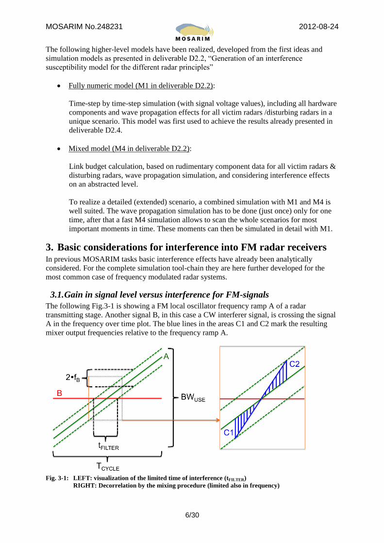
3.1. Gain in signal level versus interference for FM-signals
The following Fig.3-1 is showing a FM local oscillator frequency ramp A of a radar
transmitting stage. Another signal B, in this case a CW interferer signal, is crossing the signal
A in the frequency over time plot. The blue lines in the areas C1 and C2 mark the resulting
mixer output frequencies relative to the frequency ramp A.
Fig. 3-1: LEFT: visualization of the limited time of interference (tFILTER)
RIGHT: Decorrelation by the mixing procedure (limited also in frequency)
MOSARIM No.248231 2012-08-24
7/30
The total estimated mitigation gain in the signal-to-interference ratio from antenna port up to
the digitized data for an ideal mixer including a DFT with NFFT points [OprRoh] is
MGS/I =BWUSE
2 × fB
× NFFT =BWUSE
2 × fB
×TCYCLE
ts
(3-1)
If the sampling time tS is chosen to 1
2 × fB
, the sampling theory is satisfied and this results in
MGS/I =BWUSE
2 × fB
TCYCLE
1
2 × fB
= BWUSE ×TCYCLE (3-2)
In the case of a FMCW interfering signal and not just a CW signal, the total dwell time in the
victim receiver filter tFILTER (and by this the time per frequency bin in the FFT) can be further
increased or decreased [Gop]. This effect can be taken into account by introducing the
following scaling factor for MGS/I
SF =
BWUSE
TCYCLE
BWUSE
TCYCLE
-BWINT
TINT
(3-3)
Where MGS/I is increased if both victim and interfering ramps have different slope signs (i.e
time per frequency bin is further decreasing, resulting in less disturbed sampling points). On
the other hand, SF is decreasing when both victim and interfering ramps have the same slope
sign (i.e. time per frequency bin is increasing, with the effect to get more disturbed sampling
points).
The key to this high gain of signal-to-interference ratio is
The interference is limited to fewer sampling points.
The sampled /relevant interference contribution to the overall signal is furthermore
uncorrelated to the use-signal
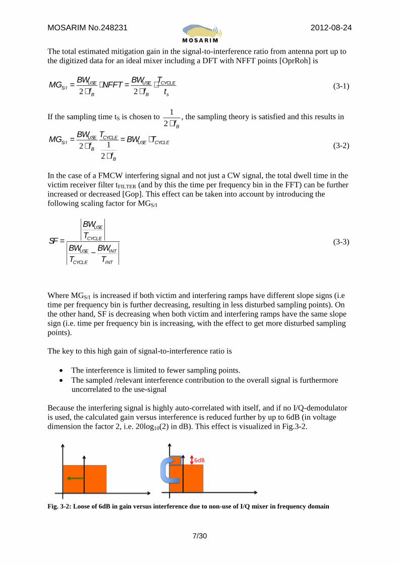
Because the interfering signal is highly auto-correlated with itself, and if no I/Q-demodulator
is used, the calculated gain versus interference is reduced further by up to 6dB (in voltage
dimension the factor 2, i.e. 20log10(2) in dB). This effect is visualized in Fig.3-2.
Fig. 3-2: Loose of 6dB in gain versus interference due to non-use of I/Q mixer in frequency domain

MOSARIM No.248231 2012-08-24
8/30
To demonstrate the equations (3-2) and (3-3), measurements have been performed for the
single interferer case. Therefore an FMCW signal with 4 MHz BW and a cycle time of 0.1 ms
is created and mixed with it’s delayed version, sampled and Fourier transformed. This results
in a target visible in the first row of the graphs in Fig. 3-3.
Fig. 3-3: Verification of the estimated interference floor in frequency domain. No I/Q data was used.
Left Column: Green=LO-signal, Red= RF-signal, Black-dotted=resulting mixer output
frequencies, magenta=3dB-filter bandwidth (magenta also marks filtered signals in time and
frequency domain)
Note: As anti-aliasing filter a Bessel 2nd
order low-pass with 120 kHz cutoff is used
In the left column in Fig.3-3, the generated mixer output frequencies are plotted. Every time
the black-dotted line (mixer output frequencies) comes close or below the magenta line (filter
3dB cut-off frequency), a peak in time domain becomes visible (middle column). These time
domain signals can be transformed into frequency domain, where an interference floor is
created which can reduce the dynamic range in a radar. The red line in the right column
indicates the predicted interference power level in frequency domain due to the changing
frequency slopes of the delayed received signal. The observed interference power level in
frequency domain for this target peak is lowered by MGS/I including the scaling factor SF
from row to row, until a CW interference is present in the second last row in Fig. 3-3. The last
row in Fig. 3-3 is showing 10 transitions through the victim’s anti aliasing filter, resulting in
the same interference power level as for the CW interference case. For the CW interfering
case we observe 20 dB gain in S/I, which corresponds to 4 MHz* 0.1 ms = 400 -> 26 dB gain
- 6 dB(no I/Q data) = 20 dB. More details about the methodology to describe multiple
interference effects can be found in deliverable D2.6.
MOSARIM No.248231 2012-08-24
9/30
3.2. Detection range in the presence of interference
Complete link budget in free space from interferer to victim radar with radiation patterns
included can be calculated as follows
PRI =PTI ×GTXI × CTI (WTI )
2×GRX × CRX(WRXI )
2×c0
2
(4p )2 RI
2 f 2 (3-4)
The radar equation can be also rewritten with normalized radiation patterns included
PRX =PTX ×GTXU × CTX(WTX )
2×GRX × CRX (WRX )
2×s ×c0
2
(4p )3 R4 × f 2 (3-5)
Assuming the change in modulation frequency is small in relation to the carrier frequency, the
signal to interference ratio including the complete interference mitigation gain MGS/I from
antenna port up to the digitized, Fourier-transformed data is given by
S
I=
PRX
PRI
=PTX
PTI
×GTXU
GTXI
×RI
2
4pR4×
CTX(WTX ) × CRX(WRX )
CTI (WTI ) × CRX(WRXI )
2
×s × MGS/I (3-6)
Legend for all equations:
PRI : received power from disturbing radar
PRX : received power from target
PTX : transmit power of victim radar
PTI : transmit power of disturbing radar
GRX : victim receive antenna gain
GTXI : disturbing radar transmit antenna gain
GTXU : victim radar transmit antenna gain
CTX : normalized radiation pattern of victim radar
TX : angle of emission of the useful signal from victim radar antenna
CTI : normalized radiation pattern of disturbing radar
TI : angle of emission of the signal from disturbing radar antenna
CRX : normalized radiation pattern of victim radar
RX : angle of incidence of the useful signal at victim radar antenna
: radar cross section of the target
R : distance from target to victim radar
RI : distance from interferer to victim radar
MGS/I : interference mitigation gain from antenna port up to the digitized data in
frequency domain
f : carrier frequency
c0 : speed of light (3*108 m/s)
Rearranging equation (3-6) for RI the maximum distance can be calculated, for which a
disturbing radar may still detect a targets under given boundary conditions and one single
propagation path (line of sight).

MOSARIM No.248231 2012-08-24
10/30
RI =S
I×PTI
PTX
×GTXU
GTXI
× 4pR4 ×CTI (WTI ) × CRX(WRXI )
CTX(WTX ) × CRX(WRX )
2
×1
s × MGS/I
(3-7)
For a target in 200m distance with an RCS of 10m2 a processing gain of 59.5dB (150MHz
bandwidth, 6ms ramp duration), omni-directional antennas, a desired minimum signal-to-
interference ratio of 12 dB and a transmit power of 20dBm EIRP pursuant to the respective
ETSI standards for both victim and interference radar, the minimum distance an interferer has
to approach the observing radar to suppress the detection of the 10 dBsm target is about 188
m for interference occurring within the main beam; the interferer is assumed to operate in CW
mode. Fig.3-4 illustrates the borders for possible target detection for several targets with RCS
from 0 to 30 dBsm (MGS/I is named GP in this figure). The formula in 3-7 will be verified in
near future by practical experiments conducted by the MOSARIM project partners. It maybe
necessary to adapt R4 to a lower value, because targets cannot be assumed to be ideally point
targets but have finite apertures which may interact with the beamwidth of the radars (i.e.
target size larger then the beamwidth in the near vicinity).
Fig. 3-4: Borders for target detection based on equation 2-11
Targets not masked by mutual/uncorrelated interference
Targets masked by
mutual/uncorrelated
interference

MOSARIM No.248231 2012-08-24
11/30
3.3. Example of a worst case scenario
Equation (3-7) is especially useful to find and define relevant interfering scenarios. Fig. 3-5 is
showing a possible worst case situation for the single interfering case.
Fig. 3-5: A small target is approaching while an LCA / BSD is disturbed by an ACC
Assuming that the bicycle does not shield the ACC yet and both interfering car and bicycle
have the same distance to the LCA (about 10 m). The LCA has the same parameters as
described in section 3.2, both LCA and ACC have the same EIRP of 20 dBm. The scaling
factor for the interference mitigation gain is assumed to be around 1. For these parameters,
Fig.3-4 shows us that the bicycle is assumed to be 12 dB above the noise level (with IQ-
receiver assumed). So it could be expected that the bicycle is around 6 dB above the noise
level in worst-case.

MOSARIM No.248231 2012-08-24
12/30
4. Modeling of relevant propagation effects
4.1. Two-path propagation
In an environment with only a victim radar and an interference radar on a road surface a two-
way propagation exists: one direct way (line-of-sight) and one indirect way with reflection via
the road surface. Fig.4-1 shows the received power at the antenna port if a two-path
propagation between two antennas with a height of 0.5 m above the ground is assumed. Fig.4-
1 shows the received power at the antenna port if a two-path propagation between two
antennas with a height of 0.5 m above the ground is assumed.
Fig. 4-1: Fading at receive antenna due to two-path propagation effect
4.2. Multipath propagation
During the test campaign in a tunnel in Utrecht, the Netherlands, on January 14th
, 2012
measurements have been performed to check the capability of the used wave propagation
simulation engine to reproduce the propagation of energy in an environment with a high
amount of multipaths. These measurements in a tunnel were also of special interest for the
project, because a significant lower path loss was expected in comparison to free-space
propagation or e.g. the propagation above a PEC half-plane. This scenario is likely to be a
worst case propagation scenario.
The measurements have been performed for a continuous wave (CW) frequency at 24.125
GHz and for all combinations of linear polarization(HH, HV, VH, VV). A vehicle’s trunk
was equipped with a signal generator and a fixed antenna (Fig.4-2b). On receive side, a
tripod device was equipped with a receiving antenna, followed by a low noise amplifier and
a spectrum analyzer to measure the received power (Fig.4-2a).
The street was sampled in steps of 100m each. The spectrum analyzer was first reset and
then set to max-hold 10m before up to 10m behind each sampling point.

MOSARIM No.248231 2012-08-24
13/30
Fig.4-3 shows the technical drawing of the tunnel in profile cut.
Fig. 4-3: Profile of the tunnel
The measurement results are visualized in Fig.4-4 and show a decoupling for cross-
polarization of about 20dB.
Fig. 4-4: Recorded (incoherent) receive power, max hold used within +/- 10 m at each 100m mark of the
tunnel
The tunnel is slightly bended towards the south end. Above 200m, the energy is already
almost equal distributed, so the bending effect is assumed to be negligible and is not
considered while modeling the tunnel. (In deliverable D1.7 [D17] this behavior is illustrated
Fig. 4-2a: non-coherent receiver, max-hold Fig. 4-2b: CW transmitter (24.125 GHz)

MOSARIM No.248231 2012-08-24
14/30
while investigating the interference potential of fixed radar device in a tunnel by simulation).
Fig. 4-5 shows the polygon-based model of the tunnel, the walls, barrier and ceiling are
modeled as concrete. Table 4-1 shows the used material parameters for simulation.
Fig. 4-5: Polygon based model of the tunnel in Utrecht
Asphalt/Concrete ε’=2.52
ε’’=0.6,
ζ=0.5 mm (standard deviation of surface height),
ζ < λ0 i)) ? if yes => flat surface for all angles of
incidence > ~40° based on Fraunhofer criterion. All other
propagation paths have additional losses due to surface
roughness and are considered by modified Fresnel
reflection factors [Geng1]. (0° is perpendicular
illumination of the street)
Concrete ε’= 2.52,
ε’’= 0,431
ζ << 0.5 mm -> negligible based on Fraunhofer criterion Tab. 4-1: Material parameters used for ray-tracing simulation
Fig.4-6 shows the comparison of the incoherent measurements using max hold and a
simulation with incoherent summation of paths for VV polarization. In addition, free-space
propagation and the two-path model are plotted for comparison. The simulation results have
been normalized to the first measurement point for better comparison..

MOSARIM No.248231 2012-08-24
15/30
Fig. 4-6: Measurement compared to simulations (VV-polarization)
Important results of these measurements:
The roll off in this tunnel can be described quiet well by 10~12dB/decade in distance were
normal free-space path loss has 20dB/decade in distance of signal attenuation. Also the used
simulation tool seems to be adequate enough to reproduce real world measurements for co-
polarization. The simulation of cross polarization (i.e. VH or HV) did not lead to a significant
correlation with measurements, because polarization changes in the simulator are always
connected to dihedral-like structures (if a polygon is defined as a reflector). Nevertheless
scatterers or scattering centers have the ability to change the polarization in a random or
deterministic way, but were not used for modelling due to the fact that the path loss behaviour
in principle is already investigated for co-polarization and can be used for worst-case
interference estimations.
MOSARIM No.248231 2012-08-24
16/30
4.3. Shielding
The shielding by road participants is also a key aspect, which has to be considered, and a
more sophisticated simulation model is able to reproduce such effects.
Because the ray-tracing tool used in the simulation tool chain supports multiple reflections,
edge-diffractions based on the uniform theory of diffraction and mixtures of both, the basic
shielding functionality is already built in and thus automatically taken into account. Fig.4-7 to
Fig.4-10 show exemplary simulations of an easy shielding scenario for 24.125 and 76.5 GHz
(polarizations: tt=vv; hh=pp). A car is moved from the transmitter to the receiver and in such
a way that line of sight is always blocked by the car. The value of shielding was calculated by
creating the relation between the undisturbed propagation (free-space, no two-path assumed
here) and the propagation with the shielding car in between, assuming an empty street and
omni-directional antennas.
Fig. 4-7: Shielding behavior, no reflections from the street are allowed (diffraction of car only)
Fig. 4-8: Shielding behavior, reflection, diffraction and combinations of both are allowed.

MOSARIM No.248231 2012-08-24
17/30
Fig. 4-9: Shielding behavior, no reflections from the street are allowed (diffraction of car only)
Fig. 4-10: Shielding behavior, reflection, diffraction and combinations of both are allowed.
The materials used for these simulations were metal for the car outline, glass for the car
window (60 GHz, e’ =5.29, tan δ = 0.048; 5 GHz, e’ = 6, tan δ = 0.01) and asphalt/concrete as
it is described in section 4.2 for the modeling of the tunnel.
If only reflections were allowed, the areas marked below Fig. 4-10 will still be present, but
without fading effects (only one path is found, or two symmetric paths e.g.). Mixed paths
(reflections in combination with diffractions) lead to more propagation paths and cause the
fading in the marked areas. The same effect can be recognized for 24 and 77GHz. In relation
to frees-pace propagation, or even in relation to the two-path model (maximum of +6dB in
relation to free-space), the car within the simulation can have a negative shielding for some
positions. The reason for that is, that the car focuses energy in the direction of the receiving
Areas, which are dominated by
reflections or combinations of
reflections and diffractions
(mixed paths)
MOSARIM No.248231 2012-08-24
18/30
antenna. If this effect found in the simulations can be confirmed in practice is still to be
determined.
In the areas where diffraction is dominant, fading also occurs. When comparing Fig. 4-8 and
Fig.4-10 it can be seen that fading effects result from mixed paths (blue curve, right side), but
can also be a result of diffracted paths (blue curve, left side).
A very smooth line (negligible fading, especially for the horizontal polarization) is an
indicator for a single, but dominant propagation path.
When comparing the overall shielding behavior for 24/77 GHz, the main differences are a
faster fading behavior for 77 GHz and a higher shielding (~ +5dB) for 77 GHz in areas, where
diffraction is dominant.
5. Road scenarios considered in this deliverable
In chapter 4 it was demonstrated, that the general ability to consider multi path effects as well
as shielding effects is given by the present simulation tool. In chapter 5 common road
scenarios are investigated on their ability to preserve energy (tunnel scenario) and also
complete scenarios including environment and road participants (cars) are considered.
In this chapter the received interference power at the antenna port is calculated for a simple
test setup. The complexity of this test scenario is continuously increased and the results are
displayed for the different frequency ranges and exemplary antennas. All scenarios contain
only one victim car and one interfering car, both equipped with 3 radars (24 GHz, 1 ACC, 2
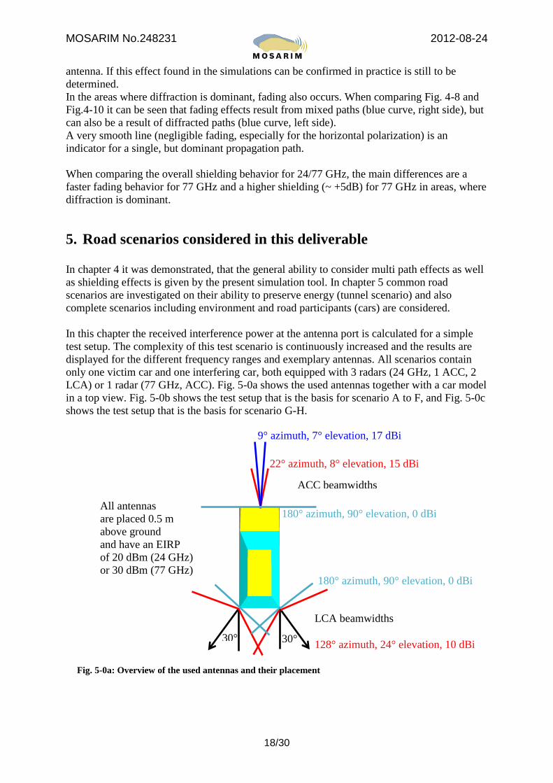
LCA) or 1 radar (77 GHz, ACC). Fig. 5-0a shows the used antennas together with a car model
in a top view. Fig. 5-0b shows the test setup that is the basis for scenario A to F, and Fig. 5-0c
shows the test setup that is the basis for scenario G-H.
30° 30°
All antennas
are placed 0.5 m
above ground
and have an EIRP
of 20 dBm (24 GHz)
or 30 dBm (77 GHz)
LCA beamwidths
128° azimuth, 24° elevation, 10 dBi
22° azimuth, 8° elevation, 15 dBi
9° azimuth, 7° elevation, 17 dBi
ACC beamwidths
Fig. 5-0a: Overview of the used antennas and their placement
180° azimuth, 90° elevation, 0 dBi
180° azimuth, 90° elevation, 0 dBi

MOSARIM No.248231 2012-08-24
19/30
In the following five different scenarios are briefly presented. They are used to check if the
gathered scenarios out of deliverable D2.2 [D12] can be seen as worst-case scenarios for the
single interference case. If this is true, equation (3-7) can be used to estimate the distance an
interferer has to approach a victim radar to become relevant.
5.1. A: Close passing
Two cars are passing each other in a near distance of 1 m. The scenario is shown in Fig. 5-1.
The starting distance is 500 m. The cars have the same speed and meet at 250 m distance.
Fig. 5-1: Scenario A, a basic scenario. No shielding, two-path only
1 m
Victim
Interferer
Fig. 5-0b: Basic setup for scenarios A-F
Victim
Interferer
Starting distance: 500 m
20 m
Speed 1
Speed 1
Road Surface
Fig. 5-0c: Basic setup for scenario G-H
Interferer
Starting distance: 250 m
20 m Speed 1 (relative)
Road Surface
Victim

MOSARIM No.248231 2012-08-24
20/30
5.2. B: Close passing – additional shielding / reflection by cars
Scenario A is modified by placing cars in 50 m steps in front and after the victim / interferer.
Fig. 5-2: Scenario B, influence of road participants in rural environment (a few multipaths occur)
5.3. C: Close passing – canyon
Scenario B is changed by adding concrete walls on both sides of the street to increase the
number of multipaths. The walls are covering 500 m of the street.
Fig. 5-3: Scenario C, a canyon like structure, as it can be found in cities or also in nature

MOSARIM No.248231 2012-08-24
21/30
5.4. D: Close passing – tunnel
The canyon from scenario C is now changed into a tunnel to further increase the amount of
multi-paths.
Fig. 5-4: Scenario D, a tunnel with centered driving lanes
5.5. E: Enlarged passing distance
Scenario D is changed by enlarging the lateral distance between the victim car and the
interferer car from 1 m to 3.5 m.
Fig. 5-5: Scenario E, more space between driving lanes in the tunnel

MOSARIM No.248231 2012-08-24
22/30
5.6. F: Close passing with guardrail
A guardrail is inserted in addition to scenario-setup D.
Fig. 5-6: The guardrail in a tunnel effectively shields interference from oncoming vehicles.
5.7. G: Tailgating a car in front
Victim and interferer car are now placed on the same lane. One of both is fixed in position,
and the other is approaching from 250 m distance.
Fig. 5-7: Approaching a car on same lane

MOSARIM No.248231 2012-08-24
23/30
5.8. H: Tailgating a car in front with guardrail
The same as described in scenario G, just a guardrail is added.
Fig. 5-8: An additional guard rail is inserted in relation to Fig. 5-7
6. Simulation results
The results are coded in the following way:
Scenario ID: victim radar <-> interfering radar , additional information.
E.g. A: ACC <-> LCA-BR/BL would mean it displays the incoherent addition of interference
powers from two LCA radars (BR= back right mounted, BL= back left mounted). The
environment used is scenario A.
If no extra information about polarization for receive or transmit antennas is mentioned within
graphics, always horizontal polarization (hh-pol. or also called pp-pol.) is plotted.

MOSARIM No.248231 2012-08-24
24/30
6.1. Results for 24 GHz ACC operation
Fig. 6-1a shows the incoherent received interference power at the victim receiver’s antenna
port. For this simulation run only the ACC radars are active.
Fig. 6-1a: The received interference power at the victim antenna port as a function of a driven distance.
Both cars are passing each other at 250 m.
When observing Fig. 6-1 it can be clearly seen that there is no difference between the five
scenario setups A-E in terms of maximum incoherent received interference power. Additional
cars on the street without walls or ceilings lead to a great shielding effect for larger distances
(blue curve, rural). Remarkable is, that the canyon (green) only brings the power levels back
from the rural scenario (blue) to the two-path propagation case (red), although we used
optimal polarization for the propagation in H-plane (hard polarization for outer car edges).
The increase of the distance between the driving lane leads to a significant reduction of the
maximum received interference power due to the smaller overlapping of the two radar main
beam lobes. On the other hand, the received interference power in greater distances is
increased, because the number of possible propagation paths between the cars is also
increased.
Fig. 6-1b shows the aggregated incoherent received interference power at the 24 GHz victim
ACC radar which is caused by the both LCA sensors of the interfering car in front of the
victim car. Basis for the simulations are scenarios G and H. In near vicinity the antenna beam
width helps to mitigate interference power in relation to a fictive omni-directional antenna
with still the same antenna gain. The guardrail increased the received interference power for
large and medium distances.

MOSARIM No.248231 2012-08-24
25/30
Fig. 6-1b: The Antenna beamwidths effectively reduce the received power in near vicinity.
All radars are operating at 24.125 GHz
6.2. Results for 24 GHz LCA operation
Fig. 6-2a shows the incoherent received interference power at the victim receiver’s antenna
port for horizontal polarization on transmit and receive. For this simulation run it is assumed
that only LCA radars are active. Both victim LCA radars receive the incoherent sum of both
interfering LCA radars.
Fig. 6-2a: The maximum received interference power is clearly be dominated by the line of sight / two-
path propagation in near vicinity. All radars are operating at 24.125 GHz
We see almost the same behavior as in section 6.1, but the maximum power levels are slightly
higher (-33.74 dBm at the antenna port of an LCA in Fig. 6-2a, -39.69 dBm at the antenna
port of the ACC in Fig. 6-1b). For the ACC versus ACC case we get about 20 dB less
received interference power in relation to the simulations where LCA/BSD is included. The
reason for this is, that –practically speaking- the ACC radars can never come close to each
other AND disturb each other, while their main beams are overlapping or crossing. LCA
radars come close to each other quite often, as well as they disturb each other mainly in their
main beams (e.g. if vehicles are passing each other as given in the example scenarios within
this document).

MOSARIM No.248231 2012-08-24
26/30
Additionally, the shielding potential of cars will be reduced if the antenna beam width
increases.
The basis for these results in Fig. 6-2b is scenario G, where victim and interfering cars have
swapped their positions. The graphic shows the received incoherent interference power
caused from the ACC at the both LCAs, when increasing the distance between the both
vehicles. Because the antenna setup is symmetrical, both received interference powers must
have the same level. The received interference power drops about 20 dB for a 250 m drive in
the tunnel.
Fig. 6-2b: Received interference power at both LCAs, all radars are operating at 24.125 GHz
6.3. Results for 77 GHz ACC operation
For the 77 GHz region, we focus on scenario D and F, with and without a guardrail between
the two driving lanes (as shown in Fig. 5-6). The guardrail starts from the ground and ends 20
cm above the involved antennas. Both variants are simulated for all co-polarizations and the
result is shown in Fig. 6-3.
Fig. 6-3: The incoherent received interference power from one single ACC radar for co-polarizations

MOSARIM No.248231 2012-08-24
27/30
Due to the narrow main beam of ACC radars, strong interference levels on straight streets are
rather unlikely. A guardrail or concrete wall starting from the ground can effectively shield
interference caused by oncoming traffic. Guardrails starting with some space above ground
still allow strong propagation paths and give about 3 dB less interference power compared to
scenario A conditions.
6.4. Incoherent versus coherent received interference power
Fig. 6-4a and Fig. 6-4b show the incoherent and coherent received interference powers for
scenario D, where all six 24 GHz radars are considered. The coherent summation of paths
does not change the practical worst-case interference power levels significantly in this
example. The change in displayed power levels due to coherent received signals/interference
is dominated by a few, but strongest path-contributions, if they exist.
Fig. 6-4a: Maximum received interference power in a tunnel scenario due to three disturbing 24 GHz
radars
Fig. 6-4b: Increased maximum interference power level by coherent adding up of the 24 GHz radars.
MOSARIM No.248231 2012-08-24
28/30
7. Conclusions
Changes in the simulation tool-chain are depicted in chapter 2, followed by a demonstration
of wave-propagation effects within the simulator in chapter 4. The capability to consider these
propagation effects makes it possible to use this simulator for the investigations defined in
this deliverable.
Due to the high amount of different radar systems it was necessary to derive simple equations
to estimate the interference floor in the frequency domain after the FFT. In chapter 3 some
equations were given which can be used to estimate the interference floor (eq. (3-2)(3-3)) as
well as to estimate problematic constellations of radar, target and interferer with respect to the
most important parameters (eq.(3-7)).
From all simulation-exercises running with single interference cases performed in this
deliverable, it can be concluded that the line-of-sight is dominating if present.
Only for energy-focusing environments like tunnels, street- or natural canyons we observe a
higher received interference power in comparison to the free-space/ two-path model due to
these focusing or canalization effects. However, the absolute maximum received interference
power occurs in a near distance, whereby the two-path propagation model and antenna
patterns are sufficient to describe the wave propagation.
Based on these results, the scenarios from deliverable D1.2 can be assumed to be worst-case
for the single interferer scenarios. The received mutual interference power levels are also not
high enough to drive the high frequency circuits of the FM receivers into compression or
saturation.
It turns out that sensors with wider antenna beam width (e.g. LCA, BSD, but also similar front
mounted radars) are more susceptible to interference than radars with a narrow beam width
(e.g. ACC). Radars with a narrow beam width have the advantage to get only interfered by the
few targets, equipped with radars, they are actually observing, what provides higher signal-to-
interference ratios by reducing the aggregated received interference power as well as the
chance to be exposed to interference.
If the maximum possible interference levels for the single entry case are to be estimated, there
is no need for complex wave propagation simulations. It is sufficient to apply a two-path
model and the nearest line-of-sight connection between victim radar and interfering radar.
The capability to simulate interference effects in time domain is given and demonstrated
within deliverable D3.6, whereby interference mitigation methods are applied to detect, avoid
or eliminate interference effects.
An important step towards a better understanding what really happens if all cars on the road
are equipped with radars, is included within deliverable D2.6. Here independent and realistic
street scenarios are applied and their corresponding frequency distributions will be derived,
allowing to estimate mean and worst-case interference power levels.

MOSARIM No.248231 2012-08-24
29/30
8. References
[D22] The MOSARIM Consortium, ”Generation of an interference
susceptibility model for the different radar principles,” Workpackage:
Simulation of Radar Interference Mechanisms, www.mosarim.eu, June
2010
[D24] The MOSARIM Consortium, ”Simulation setup assessment: interferer
– free space propagation – victim radar,” Workpackage: Simulation of
Radar Interference Mechanisms, www.mosarim.eu, June 2010
[D12] The MOSARIM Consortium, ”Specification of relevant scenarios,
applications and traffic conditions,” Workpackage: General Interference
Risk Assessment, www.mosarim.eu, June 2010
[OprRoh] D. Oprisan, H. Rohling, ”Analysis of Mutual Interference between
Automotive Radar Systems,” International Radar Symposium (IRS),
2005, Berlin, Germany, Sep. 2005
[Gop] M. Goppelt, H.-L. Bleocher, W. Menzel, ”Analytical investigation of
mutual interference between automotive FMCW radar sensors,”
Microwave Conference (GeMIC), 2011 Germany, Mar. 2011
[Geng1] Geng, N., Wiesbeck, W., “Planungsmethoden für die
Mobilkommunikation: Funknetzplanung unter realen physikalischen
Ausbreitungsbedingungen“, Springer 1998
[D17] The MOSARIM Consortium, ”Estimation of interference risk from
incumbent frequency users and services,” Workpackage: General
Interference Risk Assessment, www.mosarim.eu, June 2010

MOSARIM No.248231 2012-08-24
30/30
9. Abbreviations
ACC Automatic Cruise Control
BL Back left
BR Back right
BSD Blind Spot Detection
DFT Discrete Fourier Transformation
EIRP Equivalent Radiated Isotropic Power
FFT Fast Fourier Transformation
FMCW Frequency Modulated Continuous Wave
LCA Lange Change Assist
LO Local oscillator
MGS/I Interference Mitigation Gain (also named GP, but with respect to interference)
NFFT Number of FFT points
PEC Perfect Electric Conductor
pol Polarization
RF Radio Frequency
SF Scaling factor for MGS/I
HH/hh/pp horizontally polarized transmit-antenna, horizontally polarized receive antenna
VV/vv/tt vertically polarized transmit-antenna, vertically polarized receive antenna
HV/hv/pt vertically polarized transmit-antenna, horizontally polarized receive antenna
VH/vh/tp horizontally polarized transmit-antenna, vertically polarized receive antenna