reporting quality-control
TRANSCRIPT

REPORTING QUALITY CONTROL
SUPERVISOR: Ms. Nguyen Nhu Phong

Monitoring Software Reliability using StatisticalProcess Control: An Ordered Statistics Approach
Hoàng Minh Công
21200393
Nguyễn Văn Bình
21200267
Nguyễn Trường Minh
Members:
Contents
4.CONLUCSION
3.STATISTICAL PROCESS CONTROL
2.ORDERED STATISTICS
1.INTRODUCTION

1. INTRODUCTION
Software Operation T/F = Reliable
Control
ORDERED STATISTICS
Goel-Okumoto model
SPC
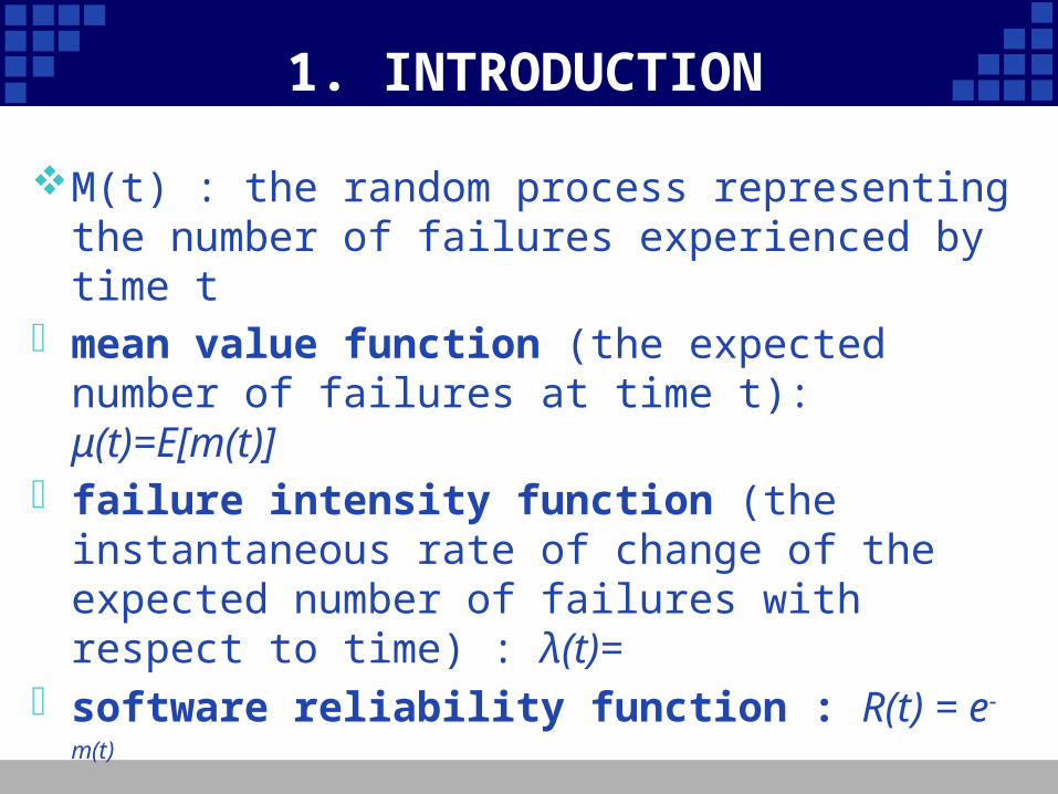
M(t) : the random process representing the number of failures experienced by time t
- mean value function (the expected number of failures at time t): μ(t)=E[m(t)]
- failure intensity function (the instantaneous rate of change of the expected number of failures with respect to time) : λ(t)=
- software reliability function : R(t) = e-m(t)
1. INTRODUCTION
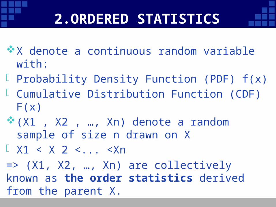
X denote a continuous random variable with:- Probability Density Function (PDF) f(x)- Cumulative Distribution Function (CDF) F(x)(X1 , X2 , …, Xn) denote a random sample of size n
drawn on X- X1 < X 2 <... <Xn
=> (X1, X2, …, Xn) are collectively known as the order statistics derived from the parent X.
2.ORDERED STATISTICS

The inter-failure time data - the time lapse between every two consecutive
failures.We can group the inter-failure time data into non
overlapping successive sub groups - size 4 or 5 - add the failure times within each sub group.The probability distribution of such a time lapse
= the rth ordered statistics in a subgroup of size r
= rth power of the distribution m (t)
2.ORDERED STATISTICS

2.ORDERED STATISTICS
Model Description
MODEL
Parameter estimation
and Control limits
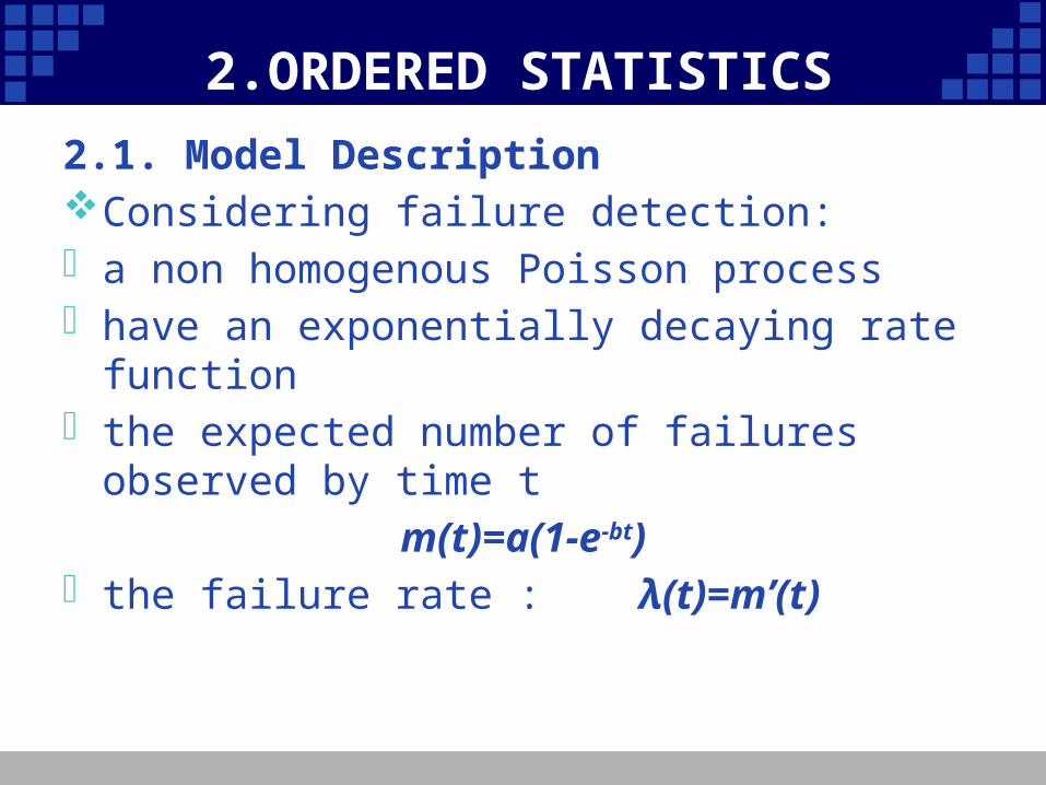
2.1. Model DescriptionConsidering failure detection:- a non homogenous Poisson process - have an exponentially decaying rate function- the expected number of failures observed by time t
m(t)=a(1-e-bt)- the failure rate : λ(t)=m’(t)
2.ORDERED STATISTICS
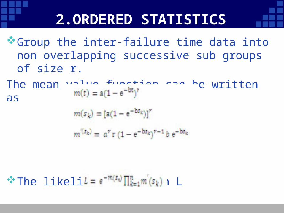
Group the inter-failure time data into non overlapping successive sub groups of size r.
The mean value function can be written as
The likelihood function L
2.ORDERED STATISTICS
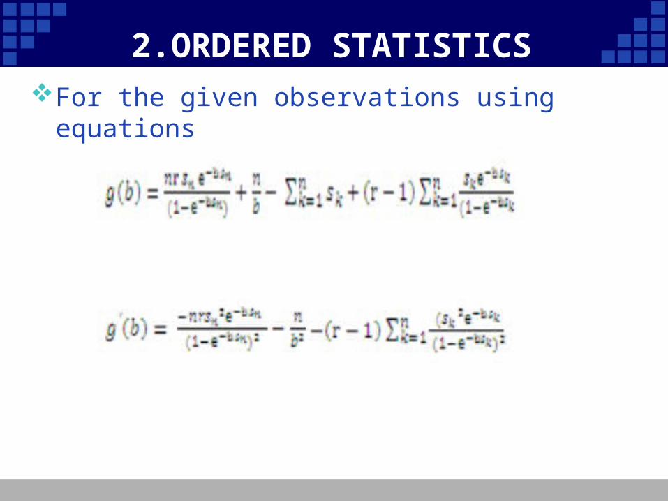
For the given observations using equations
2.ORDERED STATISTICS

2.2. Parameter estimation and Control limitsThe parameters “a” and “b” - computed by using the popular Newton Rapson
method- obtained from Goel-Okumoto model
Table 1: Parameter estimates and their control limits of 4 and 5 order Statistics
2.ORDERED STATISTICS
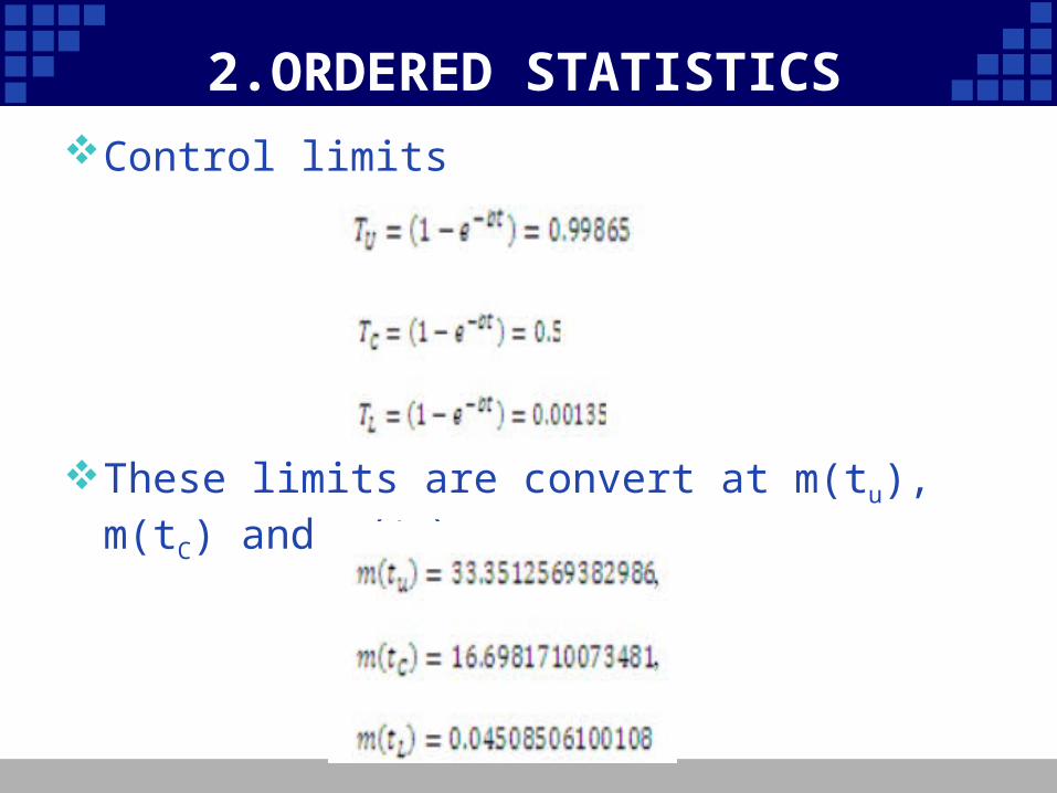
Control limits
These limits are convert at m(tu), m(tC) and m(tL)
2.ORDERED STATISTICS

3. STATISTICAL PROCESS CONTROL
Statistical process control- the application of statistical methods - provide the information necessary to continuously control - or improve processes throughout the entire lifecycle of a
product SPC techniques - help to locate trends, cycles, - irregularities within the development process and- provide clues about how well the process meets
specifications or requirements.
3. STATISTICAL PROCESS CONTROL
3.1. Control Chart
Control chart - displays sequential process measurements relative to the overall process average and control limits.
The upper and lower control limits (UCL & LCL)- establish the boundaries of normal variation for the
process being measured.- give the boundaries within which observed fluctuations
are typical and acceptable
3. STATISTICAL PROCESS CONTROL
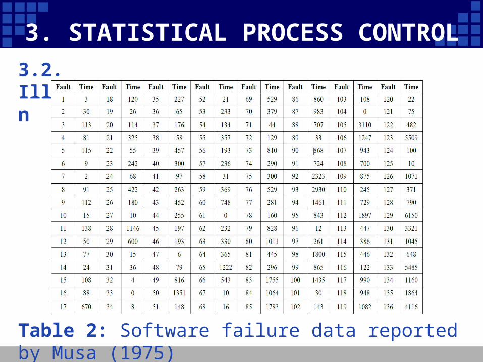
3.2. Illustration
Table 2: Software failure data reported by Musa (1975)

3. STATISTICAL PROCESS CONTROL
Table 3: 4th order cumulative faults and their m(t) successive difference.
3. STATISTICAL PROCESS CONTROL
3. STATISTICAL PROCESS CONTROL
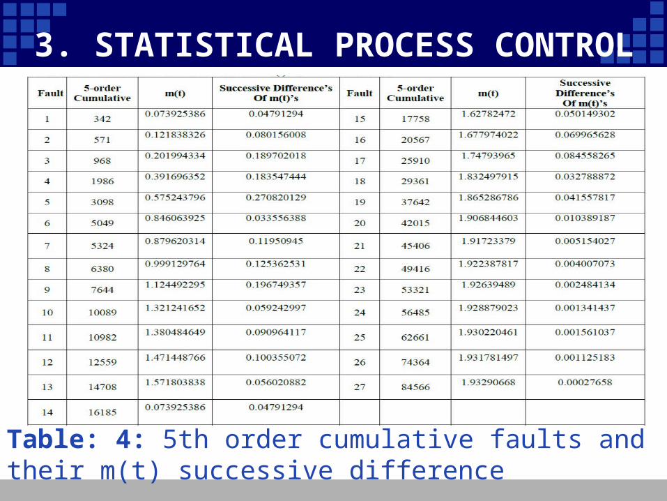
Table: 4: 5th order cumulative faults and their m(t) successive difference
3. STATISTICAL PROCESS CONTROL
4.CONCLUSION
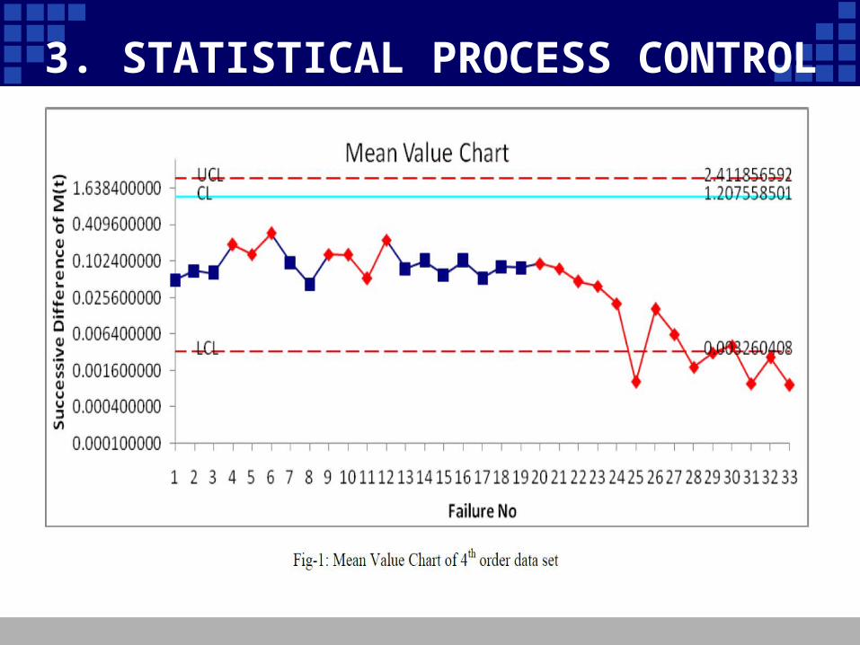
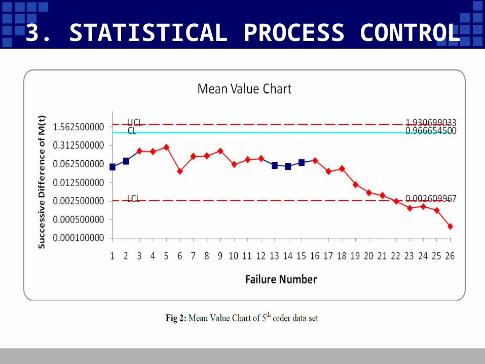
The Mean value charts of Fig 1 and 2- out of control signals i.e. below LCL. - we identified that failures situation is detected at an early
stages.The early detection of software failure will improve the
software reliability. When the control signals are below LCL- have causes leading to significant process deterioration and - it should be investigated.